Extreme value statistics of non-Markovian processes from a new class of integrable nonlinear differential equations

Abstract

This research presents a universal mapping between two key concepts in the study of stochastic processes: nonequilibrium steady-states under confinement and extreme value statistics, focusing on one-dimensional systems. The mapping holds irrespectively of the statistics of the noise driving the dynamics. This result is based on a novel approach that provides an exact trajectory-wise solution for first-order dynamics near a hard-wall boundary. I first demonstrate the applicability of this method by efficiently reproducing known results from Brownian motion theory, such as the distribution of the running maximum, and by deriving new ones, such as the survival probability below a specific curve with conditioning on the endpoint value. I then extend the analysis to non-Markovian processes, focusing on run-and-tumble particles. The mapping to a steady-state allows to compute several quantities of interest, such as the long-time probability that run-and-tumble and Brownian particles do not cross each other.

I Introduction

This work presents a mapping between two central objects in the study of stochastic processes: probability distributions in nonequilibrium steady states and extreme value statistics, in one dimension. Typical examples of nonequilibrium steady-states of interest in this work include those arising in active systems, in which individual particles dissipate internally stored energy in order to self-propel. Common models in the field are the run-and-tumble [1] and the active Orstein-Ulhenbeck [2] ones, but the domain of applicability of the mapping presented here goes beyond these two cases. In the former, in one-dimension, the dynamics of a particle is overdamped and driven by a telegraphic noise, while in the latter the dynamics is driven by a Gaussian noise which is exponentially correlated in time. The evolution of such an active particle in an external potential is generically out-of-equilibrium, a notable exception being the case of an active Ornstein-Ulhenbeck particle [3], or any particle driven by a Gaussian process [4], in a harmonic potential. The ensuing deviations from the Boltzmann weight have been the object of intense scrutiny in recent years, as active particles tend to exhibit puzzling features such as a depleted probability distribution at the bottom of an harmonic well [5] for run-and-tumble particles, and an overall tendency to be attracted to otherwise repulsive obstacles [6, 7]. Interestingly, this tendency is also exhibited in dynamics driven by memoryless non-Gaussian noises [8]. Outside equilibrium, cases for which such steady-state distribution can be obtained remain scarce, run-and-tumble particles in one-dimension being a notable exception [7].

Accordingly, and despite a broad interest in the extrema and first-passage times of non-Markovian processes [9, 10], there is no general method for studying their statistics. For non-Markovian dynamics, cases where such statistics have been analytically derived remain scarce. Run-and-tumble particles [11, 12], and models of discrete-state intermittent search strategies [13, 14], are a notable exception.

Henceforth, $\xi(t)$ denotes a stationary stochastic process with time-translation invariant statistics, which need not be Gaussian nor white. In this work, I will consider two types of stochastic evolution driven by $\xi(t)$, and relate the steady-state properties of one to the extreme value statistics of the other. In the first one, the particle is confined by a harmonic potential for $x\geq 0$ with a hard-wall at $x=0$ preventing it from accessing the $x<0$ region,

$$\dot{x}=-x+\xi(t)-W^{\prime}(x)\,.$$ (1)

Here $W$ is such that $W^{\prime}(x>0)=0$ and $W^{\prime}(x<0)=-\infty$ and accounts for the impenetrable boundary. In the second one, the particle is unconstrained, albeit driven by a noise whose amplitude decays with time,

$$\dot{y}=\text{e}^{-t}\xi(t)\,,$$ (2)

effectively maintaining the particle in the vicinity of its initial position. One of the key results of this paper is that the steady-state cumulative distribution function associated to (1) and the survival probability of (2) below a constant threshold are equal, that is

$$\mathbb{P}\left[x\leq X\right]=\mathbb{P}\left[\max_{t>0}\int_{0}^{t}\text{d}t^{\prime}\,\text{e}^{-t^{\prime}}\xi(t^{\prime})\leq X\right]\,.$$ (3)

Interestingly, the proof of this equality does not rest on probabilistic methods. Rather, it relies on the integrability of Eq. (1). In fact, despite it being strongly nonlinear, an exact solution of Eq. (1) can be obtained for any function $\xi(t)$. If $x(0)=x_{0}>0$ and if there exists $\tau_{1}>0$ such that $x(\tau_{1})=0$, then for any $t>\tau_{1}$,

$$x(t)=\max_{0<t^{\prime}<t}\int_{0}^{t^{\prime}}\text{d}\tau\,\text{e}^{-\tau}\xi(t-\tau)\,.$$ (4)

Equation (3) then follows from Eq. (4) in the steady state. An illustration of the validity of the solution in Eq. (4) is shown in Fig. 1, where the function $\xi(t)$ is taken to be a Ornstein-Ulhenbeck process (Left), a telegraphic noise (Middle) and a Gaussian white noise (Right).

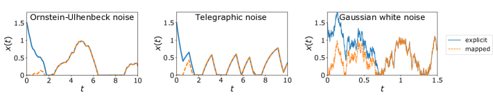
Figure 1: Dynamics of a particle confined in the vicinity of a hard wall, for different types of driving processes $\xi(t)$: an Ornstein-Ulhenbeck process (Left), a telegraphic noise (Middle) and a Gaussian white noise (Right). The explicit solution of Eq. (1) (solid, blue) is initialized at $x(0)=x_{0}=1.5>0$. After some transient ending when the trajectory of the particle hits the hard wall for the first time, the solution exactly matches the expression given in the right-hand side of Eq. (4) (orange, dashed).

The rest of the paper goes as follows. Section II is dedicated to the derivation of Eq. (4). Two derivations of this identity are actually presented, that are both instructive and could serve in the future as starting points for generalizing Eq. (3). I then discuss in Sec. III some applications of Eq. (3). I first show that it contains, as a straightforward spin-off upon a reparametrization of time, several known but scattered identities concerning the survival probability of Brownian motion, below specific curves. I then apply Eq. (3) to derive the survival probability below a constant threshold of the dynamics in Eq. (2) when $\xi(t)$ is a telegraphic noise. Lastly, I show in Sec. IV that Eq. (3) can be used to get insight into the survival probability of non-Markovian dynamics of the type $\dot{y}=\xi(t)$, in the long-time limit. As an example, I derive the long-time non-crossing probability of a run-and-tumble particle and a Brownian particle.

II Dynamics confined to the vicinity of a hard-wall: an exact solution

This section is devoted to the derivation of Eq. (4), first from a direct integration of the equation of motion Eq. (1) and then utilizing the integrability of Bernoulli equations.

II.1 From a direct integration of the equation of motion

Start by considering the nonlinear differential equation Eq. (1), with $\xi(t)$ a (piecewise) differentiable function. The initial condition is $x(0)=x_{0}$ with $x_{0}>0$. Despite its strong non-linearity, Eq. (1) can be integrated. To solve this equation, the time axis is decomposed into intervals where the particle is away from the wall and intervals where the particle sits at $x=0$. Let $\tau_{i\geq 1}$ be the sequence of successive times at which the walker hits the wall coming from the bulk and $\tilde{\tau}_{i\geq 1}$ that of successive times at which the walker leaves the wall. By definition $\tau_{i}<\tilde{\tau}_{i}<\tau_{i+1}$. If the walker is at $x=0$, it will remain so as long as $\xi(t)<0$ and will leave it as soon as $\xi(t)=0$. The underlying assumption is that there is no time $t$ such that $\xi(t)=\text{d}\xi(t)/\text{d}t=0$. Thus $\tilde{\tau}_{i}=\min_{t>\tau_{i}}(t|\xi(t)=0)$. Then, I Introduce

$$\gamma(t)\equiv x_{0}+\int_{0}^{t}d\tau\,\text{e}^{\tau}\xi(\tau)\,.$$ (5)

For $0<t<\tau_{1}$

$$x(t)=\gamma(t)\,\text{e}^{-t}$$ (6)

and thus $\tau_{1}=\text{min}_{t>0}(t|\gamma(t)=0)$. Furthermore, $x(t)=0$ for $\tau_{1}<t<\tilde{\tau}_{1}$ with $\tilde{\tau}_{1}=\min_{t>\tau_{1}}(t|\xi(t)=0)=\text{min}_{t>\tau_{1}}(t|\gamma(\tau)\text{ is a local minimum})$. For $\tilde{\tau}_{1}<t<\tau_{2}$, Eq. (1) then yields

$$x(t)=\text{e}^{-t}\,\int_{\tilde{\tau}_{1}}^{t}\text{d}\tau\,\text{e}^{\tau}\xi(\tau)=\text{e}^{-t}\left(\gamma(t)-\gamma(\tilde{\tau}_{1})\right)\,,$$ (7)

and so $\tau_{2}=\text{min}_{t>\tilde{\tau}_{1}}(t|\gamma(t)=\gamma(\tilde{\tau}_{1}))$. Accordingly,

$$\tilde{\tau}_{2}=\min_{t>\tau_{2}}(t|\gamma(t)\text{ is a local minimum})=\min_{t>0}(t|\gamma(t)\text{ is a local minimum and }\gamma(t)<\gamma(\tilde{\tau}_{1}))\,.$$ (8)

Therefore, the sequences $\tau_{i\geq 1}$ and $\tilde{\tau}_{i\geq 1}$ can be defined recursively as

$$\tau_{i+1}=\min_{t>\tilde{\tau}_{i}}(t|\gamma(t)=\gamma(\tilde{\tau}_{i}))$$ (9)

and

$$\tilde{\tau}_{i+1}=\min_{t>0}(t|\gamma(t)\text{ is a local minimum and }\gamma(t)<\gamma(\tilde{\tau}_{i}))\,.$$ (10)

In other words,

$$\tilde{\tau}_{i+1}=\operatorname*{argmin}_{0<t<\tau_{i+1}}\left(\gamma(t)\right)\,.$$ (11)

Let now $t>\tau_{1}$ such that $x(t)>0$ and let $i^{*}\geq 1$ such that $\tilde{\tau}_{i^{*}}<t<\tau_{i^{*}}$. The solution to Eq. (1) is then given by

$$x(t)=\text{e}^{-t}\left(\gamma(t)-\gamma(\tilde{\tau}_{i^{*}})\right)\,.$$ (12)

Furthermore Eqs. (9, 10) yield

$$\tilde{\tau}_{i^{*}}=\operatorname*{argmin}_{0<t^{\prime}<t}\gamma(t^{\prime})\,.$$ (13)

Hence an explicit solution is obtained as

$$x(t)=\text{e}^{-t}\,\max_{0<t^{\prime}<t}\left(\gamma(t)-\gamma(t^{\prime})\right)=\max_{0<t^{\prime}<t}\int_{0}^{t^{\prime}}\text{d}\tau\,\text{e}^{-\tau}\xi(t-\tau)\,.$$ (14)

Furthermore, note that if $x(t)=0$ for $t>\tau_{1}$, then

$$\gamma(t)=\min_{0<t^{\prime}<t}\gamma(t^{\prime})\Rightarrow\max_{0<t^{\prime}<t}\left(\gamma(t)-\gamma(t^{\prime})\right)=0\,.$$ (15)

so that

$$x(t)=\max_{0<t^{\prime}<t}\int_{0}^{t^{\prime}}\text{d}\tau\,\text{e}^{-\tau}\xi(t-\tau)\,.$$ (16)

holds in general, which demonstrates Eq. (4). Note also that for $t\geq\tau_{1}$, the system entirely loses track of its initial condition. Hence, if $x(t)$ and $y(t)$ are two realizations of Eq. (1) with the same drive $\xi(t)$ but different initial conditions, $x(0)=x_{0}$ and $y(0)=y_{0}$, then $x(t)=y(t)$ for $t>\text{max}\left(\tau_{0}^{x},\tau_{0}^{y}\right)$ with $\tau_{0}^{x}$ (accordingly $\tau_{0}^{y}$) the first time at which $x(t)=0$ (respectively $y(t)=0$).

II.2 From the integrability of Bernoulli equations

It turns out that the above derived solution can be understood as a consequence of the integrability of Bernoulli differential equations, as is shown now. First, an auxiliary process $\hat{\xi}(s)\equiv\xi(\ln s)$ is defined from the original process $\xi(t)$, which is now assumed to be a stochastic process with time-translation invariant statistics. It then appears that the correlation time of $\hat{\xi}(s)$ grows linearly with the elapsed time. The derivation proceeds by considering the Bernoulli equation,

$$\frac{\text{d}y}{\text{d}s}=-y\left(\hat{\xi}(s)+y^{n-1}\right)\,,$$ (17)

for some $n>1$. The initial conditions are such that $y(0)>0$ and so $y(s)>0$ for $s\geq 0$. It is well-known that Eq. (17) can be integrated exactly. In terms of the variable $x(s)\equiv-s^{-1}\ln y(s)$, with $x_{0}\equiv x(s_{0})$ for some $s_{0}>0$, the solution reads

$$\begin{split}x(s)&=\frac{s^{-1}}{n-1}\ln\left[\exp\left(x_{0}+(n-1)\int_{s_{0}}^{s}\text{d}s^{\prime}\hat{\xi}(s^{\prime})\right)+(n-1)\int_{s_{0}}^{s}\text{d}s^{\prime}\exp\left((n-1)\int_{s^{\prime}}^{s}\text{d}s^{\prime\prime}\hat{\xi}(s^{\prime\prime})\right)\right]\,.\end{split}$$ (18)

Reparametrizing time as $t\equiv\ln s$ yields

$$\begin{split}x(t)&=\frac{\text{e}^{-t}}{n-1}\ln\left[\exp\left(x_{0}+\text{e}^{t}\,(n-1)\int_{0}^{t-\ln s_{0}}\text{d}\tau\,\text{e}^{-\tau}\xi(t-\tau)\right)\right.\\ &\left.+(n-1)\,\text{e}^{t}\int_{0}^{t-\ln s_{0}}\text{d}\tau\,\text{e}^{-\tau}\exp\left(\,\text{e}^{t}\,(n-1)\int_{0}^{\tau}\text{d}\tau^{\prime}\,\text{e}^{-\tau^{\prime}}\xi(t-\tau^{\prime})\right)\right]\,.\end{split}$$ (19)

Now, because $\xi(t)$ has time-translation invariant correlations, the long-time behavior of $x(t)$ in (19) can be obtained by a saddle-point calculation. The result reads

$$x(t)=\max_{0<\tau<t}\int_{0}^{\tau}\text{d}\tau^{\prime}\,\text{e}^{-\tau^{\prime}}\xi(t-\tau^{\prime})\,,$$ (20)

thereby recovering the right-hand side of Eq. (4). To recover the left-hand side of Eq. (1), it remains to prove that $x(t)$ defined in this section is indeed a solution of Eq. (1) in the long-time limit. This was realized in [15] and I now recall the argument to remain self-consistent. From Eq. (17), a direct change of variable with $x(s)=-s^{-1}\ln y(s)$ and $t\equiv\ln s$ yields,

$$\dot{x}=-x+\xi(t)+\exp\left(-(n-1)\,\text{e}^{t}\,x(t)\right).$$ (21)

As $t\to\infty$, the last term vanishes for $x>0$ and diverges for $x<0$, therefore converging to the hard-wall repulsion of Eq. (1). This establishes Eq. (4).

III Applications

In this section, some applications of Eqs. (4) and (3) to extreme value statistics of stochastic processes are discussed.

III.1 Survival probabilities of Brownian motion

I start by applying Eq. (3) to the situation in which $\xi(t)$ is a Gaussian white noise. This allows me to recover the probability distribution of the maximum of Brownian motion over a finite time interval. Then, if $\xi(t)$ has a finite mean, the probability that a Brownian path starting from the origin remains below curves of the type $t\to X-a(1-\sqrt{1-t})$ for $0<t<1$ and $X>0$ is obtained, recovering earlier results proved in [16, 17].

Consider Eq. (3) in the limit where $\xi(t)=\sqrt{2}\eta(t)$ with $\eta(t)$ a zero-mean Gaussian white noise with correlations $\left\langle\eta(t)\eta(t^{\prime})\right\rangle=\delta(t-t^{\prime})$. Then the solution of Eq. (2) reads

$$y(t)=\sqrt{2}\int_{0}^{t}\text{d}t^{\prime}\,\text{e}^{-t^{\prime}}\eta(t^{\prime})\,,$$ (22)

for $t\geq 0$. By changing variables following $\tau^{\prime}=1-\text{e}^{-2t^{\prime}}$, one gets that $y(t)$ as the same statistics as the process

$$W(\tau)=\int_{0}^{\tau}\text{d}\tau^{\prime}\,\eta(\tau^{\prime})\,,$$ (23)

with $\tau=1-\text{e}^{-2t}\in[0,1]$. Here $W(\tau)$ is the standard one-dimensional Brownian motion starting at the origin. Following Eq. (3), and using that the corresponding steady-state distribution of Eq. (1) is given by the Boltzmann weight $P_{\rm{eq}}(x)=\Theta(x)\exp(-x^{2}/2)\sqrt{2/\pi}$, the distribution of the maximum of Brownian motion is recovered,

$$\mathbb{P}\left[\max_{0<\tau<1}W(\tau)\leq X\right]={\rm Erf}\left(\frac{X}{\sqrt{2}}\right)\Theta(X)\,.$$ (24)

As mentioned above, this approach can be extended to the case where $\xi(t)$ has a non-zero mean, meaning $\xi(t)=a+\sqrt{2}\eta(t)$. In that case,

$$y(t)=a\left(1-\text{e}^{-t}\right)+\sqrt{2}\int_{0}^{t}\text{d}t^{\prime}\,\text{e}^{-t^{\prime}}\eta(t^{\prime})\,,$$ (25)

and has the same statistics has

$$\hat{y}(\tau)=a\left(1-\sqrt{1-\tau}\right)+W(\tau)\,,$$ (26)

with $\tau=1-\text{e}^{-2t}\in[0,1]$. For any $X>0$, this allows to get the probability that a Brownian particle remains below the curve $t\to X-a\left(1-\sqrt{1-\tau}\right)$,

$$\mathbb{P}\left[\max_{0<\tau<1}\left(a\left(1-\sqrt{1-\tau}\right)+\int_{0}^{\tau}\text{d}\tau^{\prime}\eta(\tau^{\prime})\right)\leq X\right]=\frac{\text{Erf}\left(\frac{a}{\sqrt{2}}\right)+\text{Erf}\left(\frac{X-a}{\sqrt{2}}\right)}{\text{Erf}\left(\frac{a}{\sqrt{2}}\right)+1}\,,$$ (27)

as discussed in [16, 17]. An exemple of such non-crossing trajectory is depicted in Fig. 2.

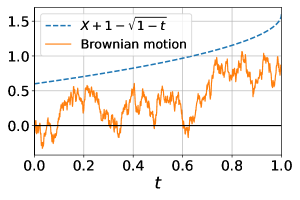
Figure 2: Illustration of a Brownian trajectory starting at the origin which remains below the curve $X+1-\sqrt{1-t}$ for any $0<t<1$. The probability of such events is given in Eq. (27) for $a=-1$.

III.2 More applications to Brownian motion from a two-time generalization of Eq. (3)

Equation (3) can be generalized at the level of two-time observables using the trajectory-wise solution Eq. (4). In turn, this allows to efficiently rederive (i) the joint distribution for the maximum and the endpoint of Brownian motion on a finite interval, (ii) the probability for a Brownian path starting at the origin to remain below the curve $X-a(1-\sqrt{1-t})$ for $X>0$ and $0<t<T$ where $T<1$, studied in [16], and (iii) the knwon probability for a Brownian path starting at the origin to remain under a shifted square-root curve [18, 19]. As a starting point, note that Eq. (4) can be rewritten as

$$\begin{split}x(t+\tau)&=\max\left\{\max_{0<t^{\prime}<\tau}\int_{0}^{t^{\prime}}\text{d}t^{\prime\prime}\text{e}^{-t^{\prime\prime}}\xi\left(t+\tau-t^{\prime\prime}\right)\,;\,\text{e}^{\tau}\max_{0<t^{\prime}<t}\int_{0}^{t^{\prime}}\text{d}t^{\prime\prime}\text{e}^{-t^{\prime\prime}}\xi\left(t-t^{\prime\prime}\right)+\int_{0}^{\tau}\text{d}t^{\prime\prime}\text{e}^{-t^{\prime\prime}}\xi\left(t+\tau-t^{\prime\prime}\right)\right\}\,,\\ &=\max\left\{\max_{0<t^{\prime}<\tau}z(t^{\prime})\,;\,\text{e}^{\tau}\,x(t)+z(\tau)\right\}\,,\end{split}$$ (28)

where

$$z(t^{\prime})\equiv\int_{0}^{t^{\prime}}\text{d}t^{\prime\prime}\text{e}^{-t^{\prime\prime}}\xi\left(t+\tau-t^{\prime\prime}\right)\,.$$ (29)

Crucially, if the dynamics is Markovian, $z(t^{\prime})$ for $t^{\prime}\in[0,\tau]$ and $x(t)$ are independent processes. Furthermore, $z(t^{\prime})$ has the same statistics as $W(\tau^{\prime})$ with $\tau^{\prime}=1-\text{e}^{-2t^{\prime}}$. Now let $P[x,\tau|x_{0}]$ be the transition probability associated to Eq. (1) in the case $\xi(t)=a+\sqrt{2}\eta(t)$. Its expression is given in terms of a series expansion, see for instance [20], which is derived in App. A for completeness,

$$P(x,t|x_{0})=\sum_{n=0}^{+\infty}\frac{1}{Z_{n}^{2}}H\left(\lambda_{n},\frac{x-a}{\sqrt{2}}\right)H\left(\lambda_{n},\frac{x_{0}-a}{\sqrt{2}}\right)\text{e}^{-\frac{x^{2}}{2}+ax}\text{e}^{-\lambda_{n}t}\,.$$ (30)

where $H(\lambda_{n},x)$ is the Hermite function. For positive integers $n$, $H(n,x)$ reduces to the Hermite polynomial of order $n$. The normalization constants is given by

$$Z_{n}^{2}=\left[\int_{0}^{+\infty}\,\text{d}x\text{e}^{-\frac{x^{2}}{2}+ax}H\left[\lambda_{n},\frac{x-a}{\sqrt{2}}\right]^{2}\right]\,,$$ (31)

and the coefficients $\lambda_{n}$ are the successive solutions of the equation

$$\lambda_{n}H\left(\lambda_{n}-1,-\frac{a}{\sqrt{2}}\right)=0\,.$$ (32)

Equating the transition probability associated to Eq. (28) with that of the constrained Ornstein-Ulhenbeck process with a drift therefore leads to the general identity,

$$\begin{split}&\mathbb{P}\left[\max_{0<t<T}\left(a\left(1-\sqrt{1-t}\right)+W(t)\right)\leq X\,;a\left(1-\sqrt{1-T}\right)+W(T)\leq X-u\right]\,\\ &=\int_{0}^{X}\text{d}x\,P\left[x,\left.-\ln\left(\sqrt{1-T}\right)\right|\frac{u}{\sqrt{1-T}}\right]\,,\end{split}$$ (33)

for any $0<T<1$. To the best of my knowledge, this identity does not exist in the literature. Several known results can be recovered from it. I will start by considering the case of a vanishing drift $a=0$, for which a simple expression for the transition probability can be obtained, for instance from the method of images or a resummation of the series in Eq. (30), see App. A. One then recovers the joint probability of the maximum and the end-point of Brownian motion over some interval $[0,T]$ as

$$\mathbb{P}\left[\max_{0<t<T}W(t)\leq X\,;W(T)\leq u\right]=\frac{1}{2}\left[{\rm Erf}\left(\frac{2X-u}{\sqrt{2T}}\right)+{\rm Erf}\left(\frac{u}{\sqrt{2T}}\right)\right]\Theta(X-u)\,.$$ (34)

I now will consider the case where $u=0$ in Eq. (LABEL:eq:identity_general), which generalizes to arbitrary times $0<T<1$ the identity shown in Eq. (27). When $u=0$, the condition at the endpoint of the interval becomes irrelevant so that

$$\mathbb{P}\left[\max_{0<t<T}\left(a\left(1-\sqrt{1-t}\right)+W(t)\right)\leq X\,\right]=\int_{0}^{X}\text{d}x\,P\left[x,\left.-\ln\left(\sqrt{1-T}\right)\right|0\right]\,.$$ (35)

Finally, I show that Eq. (LABEL:eq:identity_general) gives access to the non-crossing probability of a Brownian path with a square root curve. I first introduce the integral

$$I(X,T,u,a)\equiv\int_{0}^{X}\text{d}x\,P\left[x,\left.-\ln\left(\sqrt{1-T}\right)\right|\frac{u}{\sqrt{1-T}}\right]\,,$$ (36)

as an intermediate step. From Eq. (LABEL:eq:identity_general), one then gets,

$$\begin{split}\lim_{T\to 1}I(X,T,u,a)&=\left\langle\Theta\left[\max_{0<t<1}\left(a\left(1-\sqrt{1-t}\right)+W(t)\right)\leq X\right]\Theta\left[a+W(1)\leq X-u\right]\right\rangle\,,\\ &=\left\langle\Theta\left[\max_{0<t<1}\left(a\left(1-\sqrt{t}\right)+W(1-t)\right)\leq X\right]\Theta\left[a+W(1)\leq X-u\right]\right\rangle\,,\\ &=\left\langle\Theta\left[\max_{0<t<1}\left(a\left(1-\sqrt{t}\right)+W(1)-W(t)\right)\leq X\right]\Theta\left[a+W(1)\leq X-u\right]\right\rangle\,.\end{split}$$ (37)

Thus,

$$\begin{split}-\partial_{u}\lim_{T\to 1}I(X,T,u,a)&=\left\langle\Theta\left[\max_{0<t<1}\left(-a\sqrt{t}-W(t)\right)\leq u\right]\delta\left[a+W(1)\leq X-u\right]\right\rangle\,.\end{split}$$ (38)

Therefore

$$\mathbb{P}\left[\max_{0<t<1}\left(a\sqrt{t}+W(t)\right)\leq u\,\right]=-\int_{0}^{+\infty}\text{d}X\,\partial_{u}\left(\lim_{T\to 1}\,I(X,T,u,-a)\right)\,.$$ (39)

Using the asymptotic behavior of the Hermite functions, one then gets the expansion

$$\mathbb{P}\left[\max_{0<t<1}\left(a\sqrt{t}+W(t)\right)\leq u\,\right]=\sum_{n=1}^{+\infty}\gamma_{n}u^{\lambda_{n}-1}\,,$$ (40)

where the exponents $\lambda_{n}$ are the strictly positive roots of Eq. (32), upon replacing $a\to-a$. An explicit expression is obtained for the coefficients $\gamma_{n}$,

$$\gamma_{n}=-\lambda_{n}2^{\frac{1-\lambda_{n}}{2}}\frac{1}{Z_{n}^{2}}\int_{0}^{+\infty}\text{d}X\int_{0}^{X}\text{d}x\,H\left(\lambda_{n},\frac{x+a}{\sqrt{2}}\right)\exp\left(-\frac{x^{2}}{2}-ax\right)\,,$$ (41)

with the normalization $Z_{n}$ following from Eq. (31) upon replacing $a\to-a$. The relation in Eq. (40) leads to a power law decay of the non-crossing probability at small $u$. This is equivalent to the large-time power law decay of the non-crossing probability of a Brownian path with a square-root curve over the interval $[0,T]$ with $T$ large, as reported in [18, 19].

III.3 Non-Markovian dynamics: the example of telegraphic noise

The case of run-and-tumble particle offers a first application of Eq. (3) to non-Markovian dynamics. Indeed, for $\xi(t)=u(t)$, where $u(t)$ is a telegraphic noise switching between $1$ and $-1$ with rate $\tau^{-1}$, the steady-state distribution corresponding to the dynamics in Eq. (1) can be computed exactly using the general formula for unidimensional run-and-tumble processes [7], see App. B for a discussion of the hard-wall limit. Equation (3) then allows to derive the survival probability

$$\mathbb{P}\left[\max_{t>0}\int_{0}^{t}\text{d}t^{\prime}\,\text{e}^{-t^{\prime}}u(t^{\prime})\leq X\right]=\frac{\Gamma\left(\frac{1}{2}+\frac{1}{\tau}\right)\left(2X\,_{2}F_{1}\left(\frac{1}{2},\frac{\tau-1}{\tau};\frac{3}{2};X^{2}\right)+\tau\right)}{\tau\Gamma\left(\frac{1}{2}+\frac{1}{\tau}\right)+\sqrt{\pi}\Gamma\left(\frac{1}{\tau}\right)}\,,$$ (42)

for $0<X<1$, the same probability being equal to 1 for $X\geq 1$ since $u(t)\leq 1$ for all $t>0$. The formula in Eq. (42) perfectly agrees with numerical simulations, see Fig. 3.

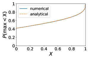
Figure 3: Agreement of the left-hand side (solid line) and right-hand side (dashed line) of Eq. (42). The continuous line was obtained by numerically sampling the maximum $\rm{max}_{t>0}\int_{0}^{t}\text{d}t^{\prime}\exp(-t^{\prime})u(t^{\prime})$. Here $\tau=3$.

IV Survival probability of unconstrained non-Markovian processes beyond the diffusive limit

When applied to a regime where the relaxation time inside the harmonic potential (which I have set to unity) is much larger than the correlation time of the noise $\xi(t)$, Eq. (3) also allows one to get predictions for the long-time survival probability of unconstrained non-Markovian processes. Let $\zeta(t)$ be some stationary random process and let

$$S(Z,T)\equiv\mathbb{P}\left[\max_{0<t<T}\int_{0}^{t}\text{d}\tau\,\zeta(\tau)\leq Z\right]\,,$$ (43)

be the corresponding survival probability over time $T$. In the following, I will assume that the dynamics $\dot{y}=\zeta(t)$ is diffusive on large scales, as it is the case for the classical run-and-tumble particles and active Ornstein-Ulhenbeck particles. As is shown next, Eq. (3) allows me to express the large time limit of $S(Z,T)$ at fixed $Z$ in terms of the steady-state density $\phi(z)$ of non-interacting particles evolving in the vicinity of a hard wall according to

$$\dot{z}=\zeta(t)-W^{\prime}(z)$$ (44)

with the boundary condition $\phi(+\infty)=1$. The result reads

$$S(Z,T)\underset{T\to\infty}{\sim}\sqrt{\frac{\beta}{T\pi}}\,\int_{0}^{Z}\text{d}z\,\phi(z)\,.$$ (45)

with $\beta^{-1}=\int_{0}^{+\infty}\text{d}\tau\left\langle\zeta(t)\zeta(t+\tau)\right\rangle$. Before proceeding with the derivation of Eq. (45), I will first discuss two examples: the long-time survival probability of a run-and-tumble particle below a constant threshold and the long-time non-crossing probability of a run-and-tumble particle with a Brownian one. For a single run-and-tumble particle, that is for $\zeta(t)=u(t)$ where $u(t)$ is a telegraphic process with rate $\tau^{-1}$, the steady-state distribution is given by

$$\phi(z)=\frac{\tau}{2}\delta(z)+\Theta(z)\,,$$ (46)

see for instance the continuous space result of [21] in the related case of two run-and-tumbe on a ring. Notice the delta-peak accumulation at the boundary of the wall which is a prominent feature of persistent random walks in confinement. Hence, Eq. (45) predicts

$$S(Z,T)\underset{T\to\infty}{\sim}\frac{1}{\sqrt{T\tau\pi}}\left(\frac{\tau}{2}+Z\right)\,,$$ (47)

in agreement with [6]. This result illustrates the direct correspondence between the delta-peak accumulation in the nonequilibrium steady-state close to a wall and the non-vanishing of the survival probability when $Z\to 0$. Next, I investigate the long-time non-crossing probability of a run-and-tumble particle with a Brownian one. This result is based on the steady-state distribution of particles close to a wall driven by both telegraphic and Gaussian white noises, which is derived in App. C. For an initial separation $Z>0$, the result reads

$$\begin{split}&\mathbb{P}\left[\max_{0<t<T}\left(\int_{0}^{t}\text{d}t^{\prime}\,u(t^{\prime})+\sqrt{2D}\int_{0}^{t}\text{d}t^{\prime}\,\eta(t^{\prime})\right)\leq Z\right]\\ &\underset{T\to\infty}{\sim}\sqrt{\frac{1}{T(D+\tau)\pi}}\left[Z+\frac{\tau}{2\sqrt{1+2D/\tau}}\left(1-\exp\left(-\sqrt{\frac{1}{D^{2}}+\frac{2}{D\tau}}\,Z\right)\right)\right]\,.\end{split}$$ (48)

An example of such a pair of non-crossing trajectories is depicted in Fig. 4.

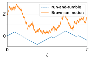
Figure 4: Illustration of a Brownian trajectory and a run-and-tumble trajectory, initially separated by a distance $Z$, which do not intersect up to time $T$.

We can now turn to the derivation of Eq. (45). With this goal in mind, consider Eq. (3) with a short-memory noise $\xi(t)\equiv\sqrt{\omega}\,\zeta(\omega t)$ where $\omega$ is a large parameter. As $\omega$ is sent to infinity, $\xi(t)$ converges to a Gaussian white noise, $\lim_{\omega\to\infty}\xi(t)=\sqrt{2\beta^{-1}}\,\eta(t)$. I will first relate the steady-state distribution in the left-hand side of Eq. (3) to the steady-state distribution in the right-hand side of Eq. (45). After that, I will relate the cumulative distribution of the maximum in the right-hand side of Eq. (3) to the cumulative distribution of the maximum in the left-hand side of Eq. (45), thereby establishing Eq. (45).

To proceed with the steady-state distributions, note that to leading order as $\omega\to\infty$, and for any $x$ finite, the steady-state probability distribution of Eq. (1) converges to the Boltzmann weight

$$P(x)=\sqrt{\frac{2\beta}{\pi}}\text{e}^{-\beta\frac{x^{2}}{2}}\Theta(x)\,.$$ (49)

Let us now probe the behavior of Eq. (1) over short scales $x=z/\sqrt{\omega}$ with $z$ finite, namely in the immediate vicinity of the confining wall where the deviations to the Boltzmann weight are the most pronounced. Upon rescaling $\tau=\omega t$ the dynamics in Eq. (1) becomes

$$\frac{\text{d}z}{\text{d}\tau}=-\frac{z}{\omega}+\eta(\tau)-W^{\prime}(z)\,.$$ (50)

Therefore, to leading order in $\omega$ at finite $z$, the steady-state distribution $P(z)$ becomes proportional to the distribution $\phi(z)$ obtained in the absence of a harmonic confinement. The proportionality constant has to be such that the distribution $P(z)$ when $z\to\infty$ matches the distribution in Eq. (49) when $x\to 0$, so that to leading order

$$P(z)=\sqrt{\frac{2\beta}{\omega\pi}}\phi(z)\,,$$ (51)

where the $1/\sqrt{\omega}$ factor comes from the Jacobian when going from $z$ to $x$.

I will now conclude by showing the correspondence between the right-hand-side of Eq. (3) and $S(Z,T)$ defined in Eq. (43). Recall that $\xi(t)=\sqrt{\omega}\,\zeta(\omega t)$ so that the right-hand side of Eq. (3) becomes

$$\begin{split}\mathbb{P}\left[\max_{t>0}\int_{0}^{t}\text{d}\tau\,\text{e}^{-\tau}\xi(\tau)\leq X\right]&=\mathbb{P}\left[\max_{t>0}\int_{0}^{t}\text{d}\tau\,\zeta(\tau)\text{e}^{-\frac{\tau}{\omega}}\leq Z\right]\,.\end{split}$$ (52)

with $Z=\sqrt{\omega}X$. It is clear that the right-hand side of Eq. (52) goes to 0 as $\omega\to\infty$, but care is required to extract the $1/\sqrt{\omega}$ leading-order behavior. Let $\epsilon>0$ be some finite number, so that

$$\begin{split}&\mathbb{P}\left[\max_{t>0}\int_{0}^{t}\text{d}\tau\,\zeta(\tau)\text{e}^{-\frac{\tau}{\omega}}\leq Z\right]\\ &=\mathbb{P}\left[\max_{0<t<\epsilon\omega}\int_{0}^{t}\text{d}\tau\,\zeta(\tau)\text{e}^{-\frac{\tau}{\omega}}\leq Z\right]\mathbb{P}\left[\left.\max_{t>\epsilon\omega}\int_{0}^{t}\text{d}\tau\,\zeta(\tau)\text{e}^{-\frac{\tau}{\omega}}\leq Z\right|\max_{0<t<\epsilon\omega}\int_{0}^{t}\text{d}\tau\,\zeta(\tau)\text{e}^{-\frac{\tau}{\omega}}\leq Z\right]\,.\end{split}$$ (53)

As shown next, the conditional probability in the right-hand side of the above equation admits a finite limit when $\omega\to+\infty$,

$$I\equiv\lim_{\omega\to\infty}\mathbb{P}\left[\left.\max_{t>\epsilon\omega}\int_{0}^{t}\text{d}\tau\,\zeta(\tau)\text{e}^{-\frac{\tau}{\omega}}\leq Z\right|\max_{0<t<\epsilon\omega}\int_{0}^{t}\text{d}\tau\,\zeta(\tau)\text{e}^{-\frac{\tau}{\omega}}\leq Z\right]\,.$$ (54)

To find the value of $I$, note that

$$\begin{split}\max_{t>\epsilon\omega}\int_{0}^{t}\text{d}\tau\,\zeta(\tau)\text{e}^{-\frac{\tau}{\omega}}&=\int_{0}^{\epsilon\omega}\text{d}\tau\zeta(\tau)\text{e}^{-\frac{\tau}{\omega}}+\max_{t>\epsilon\omega}\int_{\epsilon\omega}^{t}\text{d}\tau\,\zeta(\tau)\text{e}^{-\frac{\tau}{\omega}}\\ &=\sqrt{\omega}\int_{0}^{\epsilon\omega}\text{d}\tau\,\sqrt{\omega}\,\zeta(\omega\tau)\text{e}^{-\tau}+\sqrt{\omega}\,\text{e}^{-\epsilon}\max_{t>0}\int_{0}^{t}\text{d}\tau\,\sqrt{\omega}\,\zeta(\omega(\epsilon+\tau))\text{e}^{-\tau}\,.\end{split}$$ (55)

Therefore,

$$\begin{split}I&=\lim_{\omega\to\infty}\mathbb{P}\left[\left.\max_{t>0}\int_{0}^{t}\text{d}\tau\,\sqrt{\omega}\,\zeta(\omega(\epsilon+\tau))\text{e}^{-\tau}\leq\frac{\text{e}^{\epsilon}Z}{\sqrt{\omega}}-\text{e}^{\epsilon}\int_{0}^{\epsilon}\text{d}\tau\,\sqrt{\omega}\,\zeta(\omega\tau)\text{e}^{-\tau}\right|\max_{0<t<\epsilon}\int_{0}^{t}\text{d}\tau\,\sqrt{\omega}\,\zeta(\omega\tau)\text{e}^{-\tau}\leq\frac{Z}{\sqrt{\omega}}\right]\,.\end{split}$$ (56)

As mentioned before, $\sqrt{\omega}\zeta(\omega t)$ converges to a Gaussian white noise with effective temperature $1/\beta$ when $\omega\to\infty$. Therefore,

$$I=\lim_{a\to 0}\mathbb{P}\left[\left.\max_{0<t<1}W_{1}(t)\leq\text{e}^{\epsilon}a-\text{e}^{\epsilon}\,W_{2}(\tau_{\epsilon})\right|\max_{0<t<\tau_{\epsilon}}W_{2}(t)\leq a\right]\,,$$ (57)

where $W_{1}(t)$ and $W_{2}(t)$ are two independent Brownian motion, $a$ is a regularizing parameter and $\tau_{\epsilon}=1-\text{e}^{-2\epsilon}$. Similarly to Sec. III.1, a reparametrization of time $\tau^{\prime}=1-\text{e}^{-2\tau}$ was used to go from integrals of the Gaussian white noise with exponential kernels to Brownian motion. The value of $I$ can then be obtained from the joint distribution of the maximum of Brownian motion and its endpoint value, see Eq. (34). It reads

$$\begin{split}I&=\int_{0}^{+\infty}\text{d}u\,\frac{u}{\tau_{\epsilon}}\exp\left(-\frac{u^{2}}{2\tau_{\epsilon}}\right){\rm Erf}\left(\frac{\text{e}^{\epsilon}u}{\sqrt{2}}\right)\,,\\ &=\frac{\text{e}^{\epsilon}}{\sqrt{\text{e}^{2\epsilon}+\tau^{-1}_{\epsilon}}}\,.\end{split}$$ (58)

Hence, from Eq. (53) together with Eq. (58) and Eq. (51), we get to leading order as $\omega\to\infty$

$$\mathbb{P}\left[\max_{0<t<\epsilon\omega}\int_{0}^{t}\text{d}\tau\,\zeta(\tau)\text{e}^{-\frac{\tau}{\omega}}\leq Z\right]\underset{\omega\to\infty}{\sim}\text{e}^{-\epsilon}\sqrt{\frac{2\left(\text{e}^{2\epsilon}+\tau^{-1}_{\epsilon}\right)\beta}{\omega\pi}}\int_{0}^{Z}\text{d}z\,\phi(z)$$ (59)

By denoting $T=\epsilon\omega$ and taking $\epsilon\to 0$, Eq. (45) is then recovered.

V Conclusion

I have discussed in this paper a universal relation between non-equilibrium steady-states of stochastic processes confined on the half-line in a harmonic potential and extreme value statistics of unconstrained processes with time-decaying drive. This relation is based on the existence of an exact solution for the dynamics in the vicinity of a hard wall, that I uncovered. This mapping was then exploited to efficiently recover standard results about the extreme value statistics of Brownian motion. It also allowed me to extract novel results about the survival probability of Brownian motion below specific curves and most importantly about extreme value statistics of non-Markovian processes.

An utmost interesting perspective lies in computing the steady-state distribution of an active Ornstein-Ulhenbeck particle in the vicinity of a hard wall and infer from it the corresponding long-time survival probability. Future research directions also include looking for extensions of Eq. (3) to other classes of stochastic processes, for instance in higher-dimension. For that, one could possibly apply ideas similar to the ones developped in Sec. II.2 to different types of nonlinear differential equations. More surprisingly perhaps, I also expect results such as Eq. (4) to be of interest in the study of collective phenomenon high-dimensional systems. Indeed, dynamics such as that of high-dimensional equilibrium [22] or active [23] hard-spheres as well as dynamics in model ecosystems with many species and random interactions between them [15] can be phrased in terms of dynamical mean-field theory equations involving the study of certain stochastic processes in the vicinity of a hard wall. The nonlinearity of such equations has so far hindered our understanding of such systems. I conjecture that the solution presented here will allow future progress.

Appendix A Transition probability for the Ornstein-Ulhbenbeck process in confinement with a drift

Consider the dynamics

$$\dot{x}=-x+a+\sqrt{2}\eta(t)-W^{\prime}(x)$$ (60)

confined to $x\geq 0$ by a hard wall accounted for by the term $W^{\prime}(x)$. The transition probability $P(x,t|x_{0})$ is a solution of

$$\begin{split}&\partial_{t}P(x,t|x_{0})=-\partial_{x}\left((a-x)P(x,t|x_{0})\right)+\partial_{x}^{2}P(x,t|x_{0})\,,\\ &\partial_{x}P(0,t|x_{0})-aP(0,t|x_{0})=0\,,\\ &P(x,0|x_{0})=\delta(x-x_{0})\,.\end{split}$$ (61)

Let $K(x,t|x_{0})\equiv\exp\left(x^{2}/2-ax\right)P(x,t|x_{0})$, so that

$$\partial_{t}K=\mathcal{L}K$$ (62)

where the operator $\mathcal{L}$ reads

$$\begin{split}&\mathcal{L}u=\text{e}^{\frac{x^{2}}{2}-ax}\left(\text{e}^{-\frac{x^{2}}{2}+ax}\,u^{\prime}\right)^{\prime}\,\\ &u^{\prime}(0)=0\,.\end{split}$$ (63)

$\mathcal{L}$ is self-adjoint for the scalar product

$$\langle u,v\rangle=\int_{0}^{+\infty}u(x)v(x)\text{e}^{-\frac{x^{2}}{2}+ax}\,\text{d}x\,.$$ (64)

Let $\phi_{n}(x)$ for $n\geq 0$ be the normalized eigenvectors of $\mathcal{L}$ with associated eigenvalue $-\lambda_{n}$, that is $\mathcal{L}\phi_{n}(x)=-\lambda_{n}\phi_{n}(x)$ with $\phi_{n}^{\prime}(0)=0$. The transition probability reads

$$P(x,t|x_{0})=\sum_{n=0}^{+\infty}\phi_{n}(x)\text{e}^{-\frac{x^{2}}{2}+ax}\text{e}^{-\lambda_{n}t}\phi_{n}(x_{0})\,.$$ (65)

The eigenvectors $\phi_{n}(x)$ satisfy

$$\phi_{n}^{\prime\prime}(x)+(a-x)\phi_{n}^{\prime}(x)+\lambda_{n}\phi_{n}(x)=0\,.$$ (66)

Enforcing that the eigenvectors must not exponentially diverge at $x\to\infty$ imposes

$$\phi_{n}(x)=\frac{1}{Z_{n}}H\left(\lambda_{n},\frac{x-a}{\sqrt{2}}\right)\,.$$ (67)

where $H(\lambda_{n},x)$ is the Hermite function, generalizing to non-integer values of $\lambda_{n}$ the Hermite polynomials, and with the normalization constant

$$Z_{n}=\left[\int_{0}^{+\infty}\text{d}x\text{e}^{-\frac{x^{2}}{2}+ax}H\left[\lambda_{n},\frac{x-a}{\sqrt{2}}\right]^{2}\right]^{\frac{1}{2}}\,.$$ (68)

The eigenvalues are such that $\phi_{n}^{\prime}(0)=0$, hence are the successive solutions of the equation

$$\lambda_{n}H\left(\lambda_{n}-1,-\frac{a}{\sqrt{2}}\right)=0\,.$$ (69)

In the special case where $a=0$, meaning in the absence of drift, the series in (65) can be resummed. For $a=0$, the eigenvalues are the positive even integers $\lambda_{n}=2n$ for $n\geq 0$. The eigenvectors are the Hermite polynomials of degree $2n$. Up to a normalization by a factor $2$, these are exactly the even eigenvectors associated to the Ornstein-Ulhenbeck dynamics in the absence of the confining wall, denoted $\phi^{\rm OU}_{n}(x)$ in the following. The transition probability thus takes the form

$$\begin{split}P(x,t|x_{0})&=2\sum_{p=0}^{+\infty}\phi^{\rm OU}_{2p}(x)\phi^{\rm OU}_{2p}(x_{0})\text{e}^{-\frac{x^{2}}{2}}\text{e}^{-2pt}\,.\\ &=\sum_{n=0}^{+\infty}\phi^{\rm OU}_{n}(x)\phi^{\rm OU}_{n}(x_{0})\text{e}^{-\frac{x^{2}}{2}}\text{e}^{-nt}+\sum_{n=0}^{+\infty}\phi^{\rm OU}_{n}(x)\phi^{\rm OU}_{n}(-x_{0})\text{e}^{-\frac{x^{2}}{2}}\text{e}^{-nt}\,,\\ &=P^{\rm OU}(x,t|x_{0})+P^{\rm OU}(x,t|-x_{0})\,,\\ &=\frac{1}{\sqrt{2\pi\left(1-\text{e}^{-2t}\right)}}\left[\exp\left(-\frac{\left(x-x_{0}\text{e}^{-t}\right)^{2}}{2\left(1-\text{e}^{-2t}\right)}\right)+\exp\left(-\frac{\left(x+x_{0}\text{e}^{-t}\right)^{2}}{2\left(1-\text{e}^{-2t}\right)}\right)\right]\,,\end{split}$$ (70)

where $P^{\rm OU}(x,t|x_{0})$ is the transition probability for the Ornstein-Ulhenbeck process in the absence of confining wall. This result could have also been obtained from the method of images.

Appendix B Steady-state distribution of one-dimensional run-and-tumble particle under confinement

Consider the dynamics

$$\dot{x}=-x+v_{0}u-W^{\prime}(x)$$ (71)

where $u$ is a telegraphic process with rate $\tau^{-1}$. To mimick the hard-wall, I will take $W(x)=x\Theta(-x)/\epsilon$ and set $\epsilon\to 0^{+}$ at the end. The steady-state distribution can be computed exactly [7] and reads

$$\begin{split}P(x)&=\frac{1}{Z}\left[\left(1-\frac{x^{2}}{v_{0}^{2}}\right)^{\frac{1-\tau}{\tau}}\Theta(x)\Theta(v_{0}-x)+\left(1-\frac{x^{2}(1+\epsilon)^{2}}{\epsilon^{2}v_{0}^{2}}\right)^{\frac{\epsilon-\tau(1+\epsilon)}{\tau(1+\epsilon)}}\Theta(-x)\Theta\left(x+\frac{\epsilon v_{0}}{1+\epsilon}\right)\right]\,,\\ &\to\frac{1}{Z}\left[\left(1-\frac{x^{2}}{v_{0}^{2}}\right)^{\frac{1-\tau}{\tau}}\Theta(x)\Theta(v_{0}-x)+\frac{v_{0}\tau}{2}\delta(x)\right]\end{split}$$ (72)

where the last line was obtained in the $\epsilon\to 0^{+}$ limit. The normalization coefficient reads

$$Z=\frac{v_{0}\tau}{2}+\frac{\sqrt{\pi}v_{0}\Gamma\left(\frac{1}{\tau}\right)}{2\Gamma\left(\frac{1}{2}+\frac{1}{\tau}\right)}\,.$$ (73)

Appendix C Boundary layer in the vicinity of a wall of run-and-tumble particles with thermal noise

Consider the dynamics

$$\dot{x}=-x+v_{0}u-W^{\prime}(x)+\sqrt{2T}\eta(t)$$ (74)

where $u$ is a telegraphic process with rate $\tau^{-1}$ and $\eta(t)$ a Gaussian white noise. As usual, the term $W(x)$ formally accounts for the presence of a hard wall. In steady-state, the probability distributions in the $u=\pm 1$ states satisfy

$$\begin{split}&T\partial_{x}^{2}P_{+}(x)-v\partial_{x}P_{+}(x)+\frac{1}{\tau}\left(P_{-}(x)-P_{+}(x)\right)=0\,,\\ &T\partial_{x}^{2}P_{-}(x)+v\partial_{x}P_{-}(x)+\frac{1}{\tau}\left(P_{+}(x)-P_{-}(x)\right)=0\,,\end{split}$$ (75)

together with the no-flux boundary conditions at the wall

$$\begin{split}&T\partial_{x}P_{+}(0)-vP_{+}(0)=0\,,\\ &T\partial_{x}P_{-}(0)+vP_{-}(0)=0\,,\end{split}$$ (76)

and the boundary conditions at infinity

$$P_{+}(\infty)=P_{-}(\infty)=\frac{1}{2}\,.$$ (77)

Let $\rho(x)=P_{+}(x)+P_{-}(x)$ be the total density and $Q(x)=P_{+}(x)-P_{-}(x)$ the polarization. This leads to

$$\begin{split}&T\partial_{x}^{2}\rho(x)-v\partial_{x}Q(x)=0\,,\\ &T\partial_{x}^{2}Q(x)-v\partial_{x}\rho(x)+\frac{2}{\tau}Q(x)=0\,,\end{split}$$ (78)

together with

$$\begin{split}&T\partial_{x}\rho(0)-vQ(0)=0\,,\\ &T\partial_{x}Q(0)-v\rho(0)=0\,.\end{split}$$ (79)

Therefore,

$$Q(x)=\frac{T}{v}\partial_{x}\rho(x)\,,$$ (80)

so that

$$\partial_{x}^{3}\rho(x)-\left(\frac{v^{2}}{T^{2}}+\frac{2}{T\tau}\right)\partial_{x}\rho(x)=0\,.$$ (81)

The boundary layer therefore takes an exponential form, with

$$\rho(x)=1+c\exp\left(-\sqrt{\frac{v^{2}}{T^{2}}+\frac{2}{T\tau}}\,x\right)\,.$$ (82)

The constant $c$ is determined by the boundary condition

$$\partial^{2}_{x}\rho(0)-\frac{v^{2}}{T^{2}}\rho(0)=0\,,$$ (83)

yielding

$$\rho(x)=1+\frac{\tau v^{2}}{2T}\exp\left(-\sqrt{\frac{v^{2}}{T^{2}}+\frac{2}{T\tau}}\,x\right)\,.$$ (84)

References

- [1] Alexandre P Solon, Michael E Cates, and Julien Tailleur. Active brownian particles and run-and-tumble particles: A comparative study. The European Physical Journal Special Topics, 224(7):1231–1262, 2015.
- [2] David Martin, Jérémy O’Byrne, Michael E Cates, Étienne Fodor, Cesare Nardini, Julien Tailleur, and Frédéric Van Wijland. Statistical mechanics of active ornstein-uhlenbeck particles. Physical Review E, 103(3):032607, 2021.
- [3] Étienne Fodor, Cesare Nardini, Michael E Cates, Julien Tailleur, Paolo Visco, and Frédéric Van Wijland. How far from equilibrium is active matter? Physical review letters, 117(3):038103, 2016.
- [4] David Martin and Thibaut Arnoulx de Pirey. Aoup in the presence of brownian noise: a perturbative approach. Journal of Statistical Mechanics: Theory and Experiment, 2021(4):043205, 2021.
- [5] Julien Tailleur and ME Cates. Sedimentation, trapping, and rectification of dilute bacteria. Europhysics Letters, 86(6):60002, 2009.
- [6] Kanaya Malakar, V Jemseena, Anupam Kundu, K Vijay Kumar, Sanjib Sabhapandit, Satya N Majumdar, S Redner, and Abhishek Dhar. Steady state, relaxation and first-passage properties of a run-and-tumble particle in one-dimension. Journal of Statistical Mechanics: Theory and Experiment, 2018(4):043215, 2018.
- [7] Alexandre P Solon, Yaouen Fily, Aparna Baskaran, Mickael E Cates, Yariv Kafri, Mehran Kardar, and J Tailleur. Pressure is not a state function for generic active fluids. Nature Physics, 11(8):673–678, 2015.
- [8] Étienne Fodor, Hisao Hayakawa, Julien Tailleur, and Frédéric van Wijland. Non-gaussian noise without memory in active matter. Physical Review E, 98(6):062610, 2018.
- [9] Alan J Bray, Satya N Majumdar, and Grégory Schehr. Persistence and first-passage properties in nonequilibrium systems. Advances in Physics, 62(3):225–361, 2013.
- [10] Satya N Majumdar, Arnab Pal, and Grégory Schehr. Extreme value statistics of correlated random variables: a pedagogical review. Physics Reports, 840:1–32, 2020.
- [11] Benjamin De Bruyne, Satya N Majumdar, and Grégory Schehr. Survival probability of a run-and-tumble particle in the presence of a drift. Journal of Statistical Mechanics: Theory and Experiment, 2021(4):043211, 2021.
- [12] Abhishek Dhar, Anupam Kundu, Satya N. Majumdar, Sanjib Sabhapandit, and Grégory Schehr. Run-and-tumble particle in one-dimensional confining potentials: Steady-state, relaxation, and first-passage properties. Phys. Rev. E, 99:032132, Mar 2019.
- [13] Olivier Bénichou, Claude Loverdo, Michel Moreau, and Raphael Voituriez. Intermittent search strategies. Reviews of Modern Physics, 83(1):81, 2011.
- [14] O Bénichou, M Coppey, M Moreau, PH Suet, and R Voituriez. A stochastic model for intermittent search strategies. Journal of physics: condensed matter, 17(49):S4275, 2005.
- [15] Thibaut Arnoulx de Pirey and Guy Bunin. Many-species ecological fluctuations as a jump process from the brink of extinction. arXiv e-prints, pages arXiv–2306, 2023.
- [16] Nabil Kahale. Analytic crossing probabilities for certain barriers by brownian motion. The Annals of Applied Probability, 18(4):1424–1440, 2008.
- [17] Dobromir P. Kralchev. Levels of crossing probability for brownian motion. Random Operators and Stochastic Equations, 16(1):79–96, 2008.
- [18] Paul L Krapivsky and Sidney Redner. Life and death in an expanding cage and at the edge of a receding cliff. American Journal of Physics, 64(5):546–552, 1996.
- [19] Tristan Gautié, Pierre Le Doussal, Satya N Majumdar, and Grégory Schehr. Non-crossing brownian paths and dyson brownian motion under a moving boundary. Journal of Statistical Physics, 177(5):752–805, 2019.
- [20] Larbi Alili, Pierre Patie, and Jesper Lund Pedersen. Representations of the first hitting time density of an ornstein-uhlenbeck process. Stochastic Models, 21(4):967–980, 2005.
- [21] A. B. Slowman, M. R. Evans, and R. A. Blythe. Jamming and attraction of interacting run-and-tumble random walkers. Phys. Rev. Lett., 116:218101, May 2016.
- [22] Alessandro Manacorda, Grégory Schehr, and Francesco Zamponi. Numerical solution of the dynamical mean field theory of infinite-dimensional equilibrium liquids. The Journal of chemical physics, 152(16), 2020.
- [23] Thibaut Arnoulx de Pirey, Alessandro Manacorda, Frédéric van Wijland, and Francesco Zamponi. Active matter in infinite dimensions: Fokker–planck equation and dynamical mean-field theory at low density. The Journal of Chemical Physics, 155(17), 2021.