Strong convexity-guided hyper-parameter optimization for flatter losses

Abstract

We propose a novel white-box approach to hyper-parameter optimization. Motivated by recent work establishing a relationship between flat minima and generalization, we first establish a relationship between the strong convexity of the loss and its flatness. Based on this, we seek to find hyper-parameter configurations that improve flatness by minimizing the strong convexity of the loss. By using the structure of the underlying neural network, we derive closed-form equations to approximate the strong convexity parameter, and attempt to find hyper-parameters that minimize it in a randomized fashion. Through experiments on 14 classification datasets, we show that our method achieves strong performance at a fraction of the runtime.

1 Introduction

A typical machine learning pipeline involves using a combination of processes that have hyper-parameters that the analyst sets. There is significant interest in automatically computing a Pareto-optimal set of hyper-parameters tailored to the problem Agrawal et al. (2019); Cowen-Rivers et al. (2022); Li et al. (2017); Bergstra et al. (2011); Bergstra and Bengio (2012); Falkner et al. (2018); Eriksson et al. (2019); Ansel et al. (2014b); Snoek et al. (2012); Hernández-Lobato et al. (2014); Swersky et al. (2014); Snoek et al. (2015); Bergstra et al. (2013). In parallel, there is a venerable line of work studying the loss landscapes of neural networks Hochreiter and Schmidhuber (1994; 1997); Hinton and Van Camp (1993); Chaudhari et al. (2019); Keskar et al. (2016); Dziugaite and Roy (2017); McAllester (1999); Neyshabur et al. (2014; 2017); Li et al. (2018); Seong et al. (2018); Dauphin et al. (2014); Choromanska et al. (2015); Zhang et al. (2021). Notably, prior work has shown the effectiveness of improving the smoothness of loss surfaces via batch normalization Santurkar et al. (2018) and filter normalization Li et al. (2018).

Hyper-parameter optimization (HPO) is well-studied, with the most popular approaches being based on Bayesian optimization Snoek et al. (2012); Hernández-Lobato et al. (2014); Swersky et al. (2014); Bergstra et al. (2013), while other work suggests alternative approaches such as random search Bergstra and Bengio (2012) and tabu search Agrawal et al. (2019). Smith (2018) discusses empirical methods to manually tune hyper-parameters based on the performance of the current system. However, although HPO has repeatedly been shown to improve learner performance Tantithamthavorn et al. (2016); Majumder et al. (2018), much applied machine learning research either does not use HPO, or uses computationally expensive methods such as grid search. Some of this reluctance to use HPO stems from the general view that it is computationally expensive. For example, Tran et al. (2020) comment, “Regardless of which hyper-parameter optimization method is used, this task is generally very expensive in terms of computational costs.” Moreover, there is a growing concern to reduce the carbon emissions from ML experiments Lacoste et al. (2019). Indeed, NeurIPS now suggests authors to report the carbon emissions from their experiments.

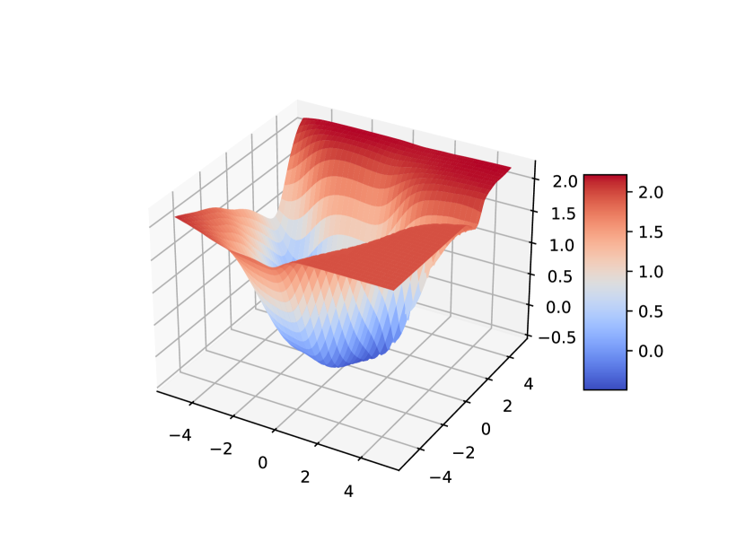
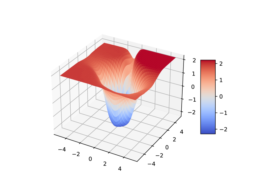
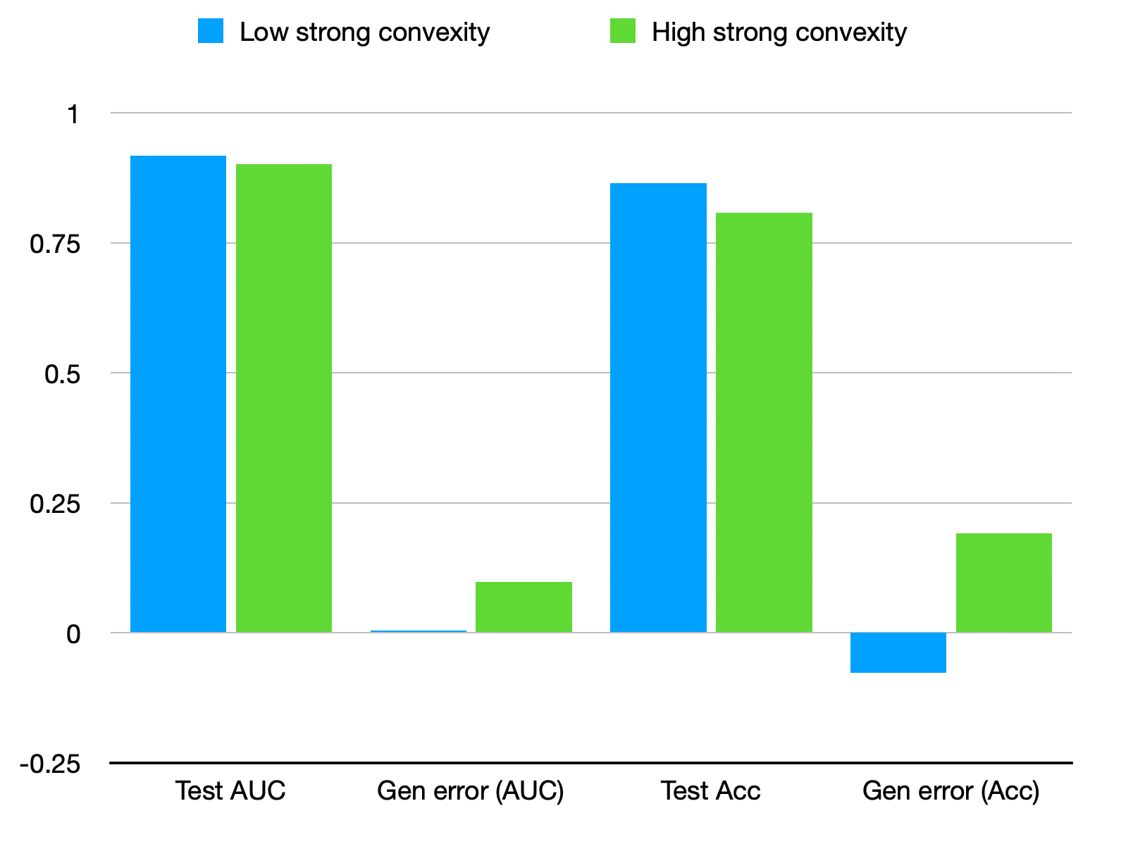
Figure 1: Landscapes (plotted using Li et al. (2018)) with their corresponding metrics, on the Australian (binary classification, imbalanced) dataset. Left: a landscape with lower strong convexity (0.112), and consequently, a wider minima. Middle: a landscape with high strong convexity (1.133), which leads to a sharp minima. Right: Test metrics and generalization error for the two hyper-parameter configurations. Although the sharper configuration converged faster to a training error of 0, it generalizes poorly and performs worse on the test set.

Motivated by the need for computationally cheaper HPO methods, we pose the following question: can we aim to directly improve the desirable properties of loss landscapes by exploiting the structure of the learning algorithm? Specifically, recent work has repeatedly endorsed the relationship between the flatness of local minima and generalization ability of networks Keskar et al. (2016); Jiang et al. (2019); Neyshabur et al. (2017); Dziugaite and Roy (2017); Li et al. (2018); Jastrzebski et al. (2017). We use four major advances in the theoretical understanding of loss landscapes: (i) Wu and Su (2023) show that SGD can escape from low-loss, sharp minima (measured by the Frobenius norm of the Hessian) exponentially fast; (ii) Dauphin et al. (2014) used the line of work starting with Bray and Dean (2007) to show that saddle points are exponentially more likely than local minima; (iii) gradient descent dynamics repel from saddle points (iv) the sharpness measure proposed by Keskar et al. (2016) have been repeatedly endorsed to correlate well with generalization Jiang et al. (2019).

In this work, we show that minimizing the supremum of the sharpness is equivalent in formulation to computing the infimum of the strong convexity of the loss in a mini-batch fashion. Next, we demonstrate a semi-empirical method of computing the strong convexity of a loss function parameterized by the hyper-parameters of the model. The result we obtain is general enough to cover a wide range of network topologies. We use this result to motivate a hyper-parameter optimization method that uses the strong convexity as a heuristic for search. Our method requires fewer full-length training runs of the learning algorithm, instead relying on one-epoch cycles to compute the strong convexity, and discarding hyper-parameter configurations that are not promising.

Figure 1 shows the motivation for our approach. The left side shows a landscape with lower strong convexity (and a flatter minima), which in turn has much lower generalization errors for both accuracy and AUC; the middle shows a landscape with a higher strong convexity (and a sharper minima), which led to a much higher generalization error for both metrics. Note that for the latter case, the training stopped early since both training AUC and accuracy reached 1; however, the model generalized poorly, and did worse on the test set.

Our contributions are as follows:

• We propose a novel white-box hyper-parameter optimization algorithm based on minimizing the strong convexity of the loss.

• We make the theoretical connection between the flatness of losses and strong convexity, motivating our approach.

• We show that our algorithm achieves strong performance in HPO across 14 datasets at a fraction of the computational cost.

To allow others to reproduce our work, our code is available online.

2 Related Work

This section briefly discusses related work; for a more comprehensive discussion, please see Appendix A.

Hyper-parameter optimization. In its general form, hyper-parameter optimization (HPO) solves the problem of finding a non-dominated hyper-parameter configuration under some budget. Early works Bergstra and Bengio (2012); Bergstra et al. (2011) showed the strength of random search, but since then, Bayesian Optimization has become increasingly popular. For example, the Tree of Parzen Estimators (TPE) algorithm models $p(x|y)$ using two kernel density estimates depending on whether $y$ is below or above some quantile, and optimizes the Expected Improvement (EI).

HyperBand (HB) Li et al. (2017) uses a procedure called “successive halving", which starts by randomly sampling a set of configurations and testing them under a limited budget, retaining only the best-performing ones and allocating those greater resources. At its core, its strategy is to aggressively prune poor-performing configurations so that more promising ones can be allocated more resources. Algorithms such as BOHB Falkner et al. (2018) and DEHB Awad et al. (2021) improve upon these in different ways: DEHB uses a distributed computing approach and combines differential evolution with HB, while BOHB combines a slightly modified version of the BO-based TPE with HB.

HEBO Cowen-Rivers et al. (2022) use a combination of input and output transformations along with NSGA-II to optimize a multi-objective acquisition function. TuRBO Dou et al. (2023) assumes the hyper-parameter to performance mapping is Lipschitz, and uses an ensemble of learners to predict performance, using the prediction to update its Gaussian Process model instead if that prediction is poor.

Flat minima and generalization. The connection between “flat minima” and generalization has been repeatedly endorsed. The flatness of minima has been defined in various ways, such as the volume of hypercuboids such that the loss is within a tolerance Hochreiter and Schmidhuber (1997) and as robustness to adversarial perturbations in weight space Keskar et al. (2016). The specific formulation of Keskar et al. (2016) is

$$\zeta(\boldsymbol{w};\epsilon)=\frac{\max\limits_{\boldsymbol{v}\in\mathcal{B}(\epsilon,\boldsymbol{w})}f(\boldsymbol{v})-f(\boldsymbol{w})}{1+f(\boldsymbol{w})}$$

This notion of sharpness was also endorsed by a large-scale study of complexity measures by Jiang et al. (2019). The relationship between flatness and generalization was later also endorsed by several works Neyshabur et al. (2017); Li et al. (2018); Wu and Su (2023). We defer the reader to Appendix A for a more detailed review.

3 Method

3.1 Notation and Assumptions

For any learner, $X\in\mathcal{X}$ will represent the independent variables and $y$ will represent the labels; $W$ represents the weights of a neural network. We use $m$ to denote the number of training samples, $n$ to denote the number of features, $k$ to denote the number of classes, and $E$ to denote the loss function.

For a feedforward network, $L$ represents the number of layers, and at each layer, the following computation is performed: $z^{[l]}=W^{[l]T}a^{[l-1]}+b^{[l]}$ and $a^{[l]}=g^{[l]}(z^{[l]})$ where $a^{[0]}=X$. Here, $b^{[l]}$ is the bias vector at layer $l$, $W^{[l]}$ is the weight matrix at layer $l$, and $g^{[l]}$ is the activation function used at layer $l$–we will assume this is the ReLU function $g^{[l]}(x)=\max(0,x)\ \forall l\in\{1,\ldots,L-1\}$.

We use $\nabla_{W}\cdot$ to denote the first gradient of $\cdot$, with respect to $W$. $\nabla^{2}_{W}\cdot$ denotes the Hessian. Finally, $\mathcal{B}(\epsilon,w)$ denotes an $\epsilon-$ball centered at $w$. Whenever unspecified, the matrix norm is the Frobenius norm. We use $\mathbb{S}^{n}$ to denote the set of $n\times n$ real, symmetric matrices. We defer to Appendix B for background definitions in convex optimization.

We assume the space $\mathcal{X}$ is Polish. We use the Frobenius norm of the Hessian to define the strong convexity of a loss landscape. In this context, completeness of the underlying metric space is necessary. Moreover, completeness is an important assumption in gradient descent, since it guarantees the existence of limits for Cauchy sequences. Finally, separability helps avoid issues with measurability when we use a covering argument in the next section.

3.2 AHSC: Accelerated HPO via Strong Convexity

Lemma 1.

Let $A,B\in\mathbb{S}^{n}$ and suppose $A\succeq B$. Then $\left\lVert A\right\rVert_{2}\geq\left\lVert B\right\rVert_{2}$

Proof.

We have $\left\lVert A\right\rVert_{2}=\sqrt{\lambda_{max}(A^{T}A)}=\left\lvert\lambda_{max}(A)\right\rvert$ since $A$ is symmetric. Since $A\succeq B$, we have by definition $x^{T}Ax\geq x^{T}Bx$ for an arbitrary $x\in\mathbb{R}^{n}$. From the min-max theorem, we have $\forall k\in\{1,\ldots,n\}$,

$$\lambda_{k}(A)=\min\limits_{\begin{subarray}{c}\mathcal{M}\subset\mathbb{S}^{n}\\ \dim\mathcal{M}=k\end{subarray}}\max\limits_{x\in\mathcal{M}\backslash\{0\}}\frac{x^{T}Ax}{x^{T}x}\geq\min\limits_{\begin{subarray}{c}\mathcal{M}\subset\mathbb{S}^{n}\\ \dim\mathcal{M}=k\end{subarray}}\max\limits_{x\in\mathcal{M}\backslash\{0\}}\frac{x^{T}Bx}{x^{T}x}=\lambda_{k}(B)$$

where $\lambda_{k}$ is the $k$th eigenvalue in the spectrum ordered in non-increasing order. Using the above with $k=1$ completes the proof. ∎

We start by writing the definition of strong convexity in terms of positive-semidefiniteness as

$$\nabla^{2}f(x)\succeq\mu I$$

From Lemma 1, we can rewrite this as

$$\lVert\nabla^{2}f(x)\rVert_{2}\geq\mu\Rightarrow\left\lVert\nabla^{2}f(x)\right\rVert_{F}\geq\mu$$

and so we redefine $\mu-$strong convexity as

$$\mu=\inf\lVert\nabla^{2}f(x)\rVert_{F}$$

A key motivation for minimizing the strong convexity is to relate it to the flatness of minima. Since $\nabla^{2}f$ is symmetric (by Schwarz’s theorem), we have

$$\left\lvert\lambda_{max}(\nabla^{2}f)\right\rvert=\left\lVert\nabla^{2}f\right\rVert_{2}\leq\left\lVert\nabla^{2}f\right\rVert_{F}$$

so that $\left\lvert\lambda_{max}(\nabla^{2}f)\right\rvert=\inf\left\lVert\nabla^{2}f\right\rVert_{F}$ which directly relates the sharpness of the landscape with the definition of strong convexity above. We can also relate the above definition of strong convexity to the sharpness measure $\zeta$ established by Keskar et al. (2016):

$$\zeta(w) =\frac{\max\limits_{w^{\prime}\in\mathcal{B}(\epsilon,w)}f(w^{\prime})-f(w)}{1+f(w)}$$

$$\overset{(i)}{\approxeq}\max\limits_{w^{\prime}\in\mathcal{B}(\epsilon,w)}f(w^{\prime})-f(w)$$

$$\overset{(ii)}{\approxeq}\frac{\epsilon^{2}}{2}\left\lVert\nabla^{2}f(w)\right\rVert_{2}\leq\frac{\epsilon^{2}}{2}\left\lVert\nabla^{2}f(w)\right\rVert_{F}$$

where (i) is because the training error is typically small in practice Neyshabur et al. (2017) and (ii) follows from a second-order Taylor expansion of $f$ around $w$, as done by Dinh et al. (2017). Therefore, we wish to minimize the sharpness, which is equivalent to the formulation above. Equivalently, we have (with $r$ denoting the rank of the Hessian)

$$\zeta(w)\approxeq\frac{\epsilon^{2}}{2}\left\lVert\nabla^{2}f(w)\right\rVert_{2}\geq\frac{\epsilon^{2}}{2\sqrt{r}}\left\lVert\nabla^{2}f(w)\right\rVert_{F}\geq\frac{\epsilon^{2}}{2\sqrt{n}}\left\lVert\nabla^{2}f(w)\right\rVert_{F}$$

so that the strong convexity is a lower bound on the sharpness, and a higher strong convexity implies a higher sharpness, which is correlated with a higher generalization error. Therefore, we have:

$$\frac{\epsilon^{2}}{2\sqrt{n}}\left\lVert\nabla^{2}f(w)\right\rVert_{F}\leq\zeta(w)\leq\frac{\epsilon^{2}}{2}\left\lVert\nabla^{2}f(w)\right\rVert_{F}$$

so that the strong convexity and a scaled version thereof provide bounds on the sharpness, and minimizing the strong convexity implies both the lower and upper bounds on the sharpness are lowered.

Motivated by the above relationship, we seek to find hyper-parameters that minimize this strong convexity. For a learner parameterized by $H\in\mathcal{H}$, denote its loss function as $E(x;H)$. Then, we would like to solve the problem

$$\inf\limits_{H\in\mathcal{H}}\sup\limits_{x\subset X}\lVert\nabla^{2}E(x;H)\rVert$$

This mini-batch version accounts for large datasets for which a mini-batch approach is necessary. Note that it is necessary to use an upper bound approximation at the mini-batch level: using an $\inf$ instead yields 0 a majority of the time, making the search ineffective. Indeed, we can relate this to the sharpness measure from Keskar et al. (2016): this formulation corresponds to minimizing the upper bound on the sharpness over the entire $\epsilon-$ball.

We can bound the deviation from the true supremum using a covering argument Duchi (2023). Let $f(x)=\sup\left\lVert\nabla^{2}E(x)\right\rVert$ be drawn from some set of functions $\mathcal{F}$, each of whose elements map from $\mathcal{X}$ to $\mathbb{R}$. Define a point-mass empirical distribution on $\{x_{i}\}_{i=1}^{m}$ as $P_{m}=\frac{1}{m}\sum\limits_{i=1}^{m}\delta_{x_{i}}$ where $\delta$ is the Dirac delta. For any function $f:\mathcal{X}\to\mathbb{R}\in\mathcal{F}$, let

$$P_{m}f\triangleq\mathbb{E}_{P_{m}}[f(X)]=\sum\limits_{i=1}^{m}f(x_{i})$$

be the empirical expectation over a mini-batch and let

$$Pf\triangleq\mathbb{E}_{P}[f(X)]=\int f(x)dP(x)$$

denote the general expectation under a measure $P$. Suppose the functions in $\mathcal{F}$ are bounded above by $\beta$ (trivially, they are bounded below by 0), and define the metric over $\mathcal{F}$ as $\left\lVert f-g\right\rVert_{\infty}=\sup\limits_{x\in\mathcal{X}}\left\lvert f(x)-g(x)\right\rvert$. Denote by $N(\delta,\Theta,\rho)$, the covering number for a $\delta-$cover of a set $\Theta$ with respect to a metric $\rho$. Then, we use the standard covering number guarantee (cf. Duchi (2023) Ch. 4) to get

Algorithm 1 shows our overall approach. We first sample $N_{1}$ random configurations (line 2). For each of these configurations, we first train the model for one epoch to bring the weights closer to their final weights (line 6). Training for a single epoch provides a balance between the cost associated with training fully (which would provide a more accurate estimate for the strong convexity), and not training at all (which provides a very poor estimate). We then compute $\left\lVert\nabla^{2}E(x)\right\rVert$ in a mini-batch fashion (lines 8-10). Since we wish to minimize the strong convexity, it is important that we look at the highest value across mini-batches, and aim to minimize that upper bound. Importantly, if the strong convexity is 0 (implying the function is not strongly convex), we discard that configuration (lines 11-13). We pick the configurations corresponding to the $N_{2}$ lowest values of strong convexity as computed above, and train those models fully (lines 15-17). Finally, we return the best-performing configuration.

In Appendix C, Theorem 2, we show that if the loss is smooth and $\mu-$strongly convex, then

$$f(x_{t})-f(x^{*})\leq(1-\alpha\mu)^{t}\left(f(x_{0})-f(x^{*})\right)$$

where $\alpha$ is the learning rate. Therefore,

$$f(x_{t+1})-f(x_{t}) \leq\left((1-\alpha\mu)^{t+1}-(1-\alpha\mu)^{t}\right)\left(f(x_{0})-f(x^{*})\right)$$

$$\leq(1-\alpha\mu)^{t}(-\alpha\mu)\left(f(x_{0})-f(x^{*})\right)$$

$$\leq\exp(-\alpha\mu t)(-\alpha\mu)\left(f(x_{0})-f(x^{*})\right)$$

which implies exponentially decaying benefit as the number of epochs increases. On the other hand, Theorem 2 also implies that for vanilla gradient descent, the number of steps required for convergence is inversely proportional to the strong convexity, so that minimizing the latter implies a greater number of steps is required to converge (which increases the runtime). To reduce the impact of this, we use the Adam Kingma and Ba (2014) optimizer. We leave it to future work to explore additional strategies, such as large adaptive learning rates, which can also lead to flatter losses Jastrzebski et al. (2017).

Input : Number of configurations to sample $N_{1}$, number of configurations to run $N_{2}$. Defaults: $N_{1}=50,N_{2}=10$

1

2$\mathcal{H}_{0}\leftarrow$ Random($\mathcal{H},N_{1}$);

$S\leftarrow\phi$ ;

  // Strong convexity values

3;

$P\leftarrow\phi$ ;

  // Performance scores

4;

5

6for config $h$ in $\mathcal{H}_{0}$ do

7       Train for one epoch using $h$;

8       $\mu_{max}=-\infty$;

9       for mini-batch $x\subset X$ do

10             $\mu_{max}=\max(\mu_{max},\left\lVert\nabla^{2}f(x;h)\right\rVert)$;

11            

12       end for

13      if $\mu_{max}>0$ then

14             S[h] $\leftarrow\mu_{max}$;

15            

16       end if

17      

18 end for

19

20for config $h$ in Lowest(S, $N_{2}$) do

21       P[h] $\leftarrow$ Run(h);

22      

23 end for

24

return $\operatorname*{arg\,max}P$

Algorithm 1 AHSC

We now consider the general multi-class classification problem, where the cross-entropy loss is used, and the last layer of the neural network uses a softmax activation. Below, we show that the strong convexity of a feedforward network with a softmax activation in the last layer, trained on the cross-entropy loss, is given by

$$\inf\left\lVert\nabla^{2}_{W}E\right\rVert\propto\frac{1}{m}\inf\frac{\lVert a_{j}^{[L-1]}\rVert}{\lVert W^{[L]}\rVert}$$

Importantly, the proof does not rely on the architecture of the network beyond the last two layers. That is, as long as the last two layers of the network are fully-connected, this theorem applies.

Lemma 2.

For a neural network with ReLU activations in the hidden layers and a softmax activation at the last layer,

$$\frac{\partial E}{\partial z^{[L]}_{j}}=\frac{1}{m}\left(\sum\limits_{i=1}^{m}[y^{(i)}=j]\right)\left(\sum\limits_{h=1}^{k}a^{[L]}_{j}-\delta_{hj}\right)$$

under the cross-entropy loss.

Proof.

We will use the chain rule, as follows:

$$\frac{\partial E}{\partial z^{[L]}_{j}} =\frac{\partial E}{\partial a^{[L]}_{j}}\cdot\frac{\partial a^{[L]}_{j}}{\partial z^{[L]}_{j}}$$ (1)

Consider the Iverson notation version of the general cross-entropy loss:

$$E(a^{[L]})=-\frac{1}{m}\sum\limits_{i=1}^{m}\sum\limits_{h=1}^{k}[y^{(i)}=h]\log a_{h}^{[L]}$$

Then the first part of (1) is trivial to compute:

$$\frac{\partial E}{\partial a_{j}^{[L]}}=-\frac{1}{m}\sum\limits_{i=1}^{m}\frac{[y^{(i)}=j]}{a_{j}^{[L]}}$$ (2)

The second part is the derivative of the softmax and is equal to

$$\frac{\partial a^{[L]}_{j}}{\partial z^{[L]}_{p}} =a^{[L]}_{j}([p=j]-a^{[L]}_{p})$$ (3)

Combining (2) and (3) in (1) gives

$$\frac{\partial E}{\partial z^{[L]}_{j}}=\frac{1}{m}\left(\sum\limits_{i=1}^{m}[y^{(i)}=j]\right)\left(\sum\limits_{h=1}^{k}a^{[L]}_{j}-\delta_{hj}\right)$$ (4)

∎

Theorem 1 ($\mu-$strong convexity for neural classifiers).

For a neural network with ReLU activations in the hidden layers, a fully connected penultimate layer, and a softmax activation at the last layer, the $\mu-$strong convexity of the cross-entropy loss is given by

$$\inf\left\lVert\nabla^{2}_{W}E\right\rVert\propto\frac{1}{m}\inf\frac{\lVert a_{j}^{[L-1]}\rVert}{\lVert W^{[L]}\rVert}$$ (5)

Proof.

For a neural network with ReLU activations, Lemma 2 gives us (using the chain rule one step further):

$$\nabla_{W^{[L]}_{j}}E=\frac{1}{m}\left(\sum\limits_{i=1}^{m}[y^{(i)}=j]\right)\left(\sum\limits_{h=1}^{k}a^{[L]}_{j}-\delta_{hj}\right)a_{j}^{[L-1]}$$

Therefore,

$$\nabla^{2}_{W^{[L]}_{j}}E =\frac{1}{m}\left(\sum\limits_{i=1}^{m}[y^{(i)}=j]\right)\left(\sum\limits_{h=1}^{k}a^{[L]}_{j}-\delta_{hj}\right)\nabla_{W^{[L]}_{j}}a_{j}^{[L-1]}$$

$$=\frac{1}{m}\left(\sum\limits_{i=1}^{m}[y^{(i)}=j]\right)\left(\sum\limits_{h=1}^{k}a^{[L]}_{j}-\delta_{hj}\right)\dfrac{\partial a_{j}^{[L-1]}}{\partial E}\dfrac{\partial E}{\partial W^{[L]}_{j}}$$

$$=\frac{1}{m^{2}}\left(\sum\limits_{i=1}^{m}[y^{(i)}=j]\right)^{2}\left(\sum\limits_{h=1}^{k}a_{j}^{[L]}-[h=j]\right)^{2}\frac{\partial a_{j}^{[L-1]}}{\partial E}a_{j}^{[L-1]}$$

$$=\frac{1}{m^{2}}\left(\sum\limits_{i=1}^{m}[y^{(i)}=j]\right)^{2}\left(\sum\limits_{h=1}^{k}a_{j}^{[L]}-[h=j]\right)^{2}\frac{1}{\dfrac{\partial E}{\partial a_{j}^{[L-1]}}}a_{j}^{[L-1]}$$

Using $z^{[l]}=W^{[l]T}a^{[l-1]}+b^{[l]}$ and Lemma 2 gives us:

$$\dfrac{\partial E}{\partial a_{j}^{[L-1]}} =\dfrac{\partial E}{\partial z_{j}^{[L]}}\dfrac{\partial z_{j}^{[L]}}{\partial a_{j}^{[L-1]}}$$

$$=\frac{1}{m}\left(\sum\limits_{i=1}^{m}[y^{(i)}=j]\right)\left(\sum\limits_{h=1}^{k}a_{j}^{[L]}-[h=j]\right)W_{j}^{[L]}$$

The limiting case of this is when all softmax values are 0, so that the second summation term is -1. The first summation is a positive constant, which we drop as a proportionality constant. Now, (5) immediately follows. ∎

4 Experiments

Table 1: Experimental results on various classification datasets. AHSC is our method. Values shown are medians over 20 repeats. Statistically best results are highlighted in bold (see Section 4 for details).

Image
Dataset	HPO method	Accuracy
MNIST	AHSC	98.65
	Hyperopt	97.22
	Random	98.95
	TuRBO	98.99
	HEBO	98.94
	BOHB	98.85
SVHN	AHSC	86.63
	Hyperopt	67.20
	Random	91.86
	TuRBO	80.41
	HEBO	92.89
	BOHB	79.67
Bayesmark
Dataset	HPO method	Score
breast	AHSC	93.98
	Hyperopt	92.68
	Random	90.45
	TuRBO	88.97
	HEBO	90.84
	BOHB	92.37
digits	AHSC	84.74
	Hyperopt	96.85
	Random	87.39
	TuRBO	89.51
	HEBO	95.24
	BOHB	91.50
iris	AHSC	91.00
	Hyperopt	79.83
	Random	82.98
	TuRBO	83.52
	HEBO	78.27
	BOHB	92.30
wine	AHSC	92.35
	Hyperopt	83.98
	Random	76.59
	TuRBO	81.15
	HEBO	74.93
	BOHB	81.68

OpenML
Dataset	HPO method	AUC
vehicle	AHSC	0.885
	Hyperopt	0.883
	Random	0.873
	TuRBO	0.882
	HEBO	0.884
	BOHB	0.883
blood-transf…	AHSC	0.721
	Hyperopt	0.728
	Random	0.708
	TuRBO	0.720
	HEBO	0.718
	BOHB	0.725
Australian	AHSC	0.934
	Hyperopt	0.932
	Random	0.928
	TuRBO	0.932
	HEBO	0.935
	BOHB	0.928
car	AHSC	1.0
	Hyperopt	1.0
	Random	1.0
	TuRBO	1.0
	HEBO	1.0
	BOHB	1.0
phoneme	AHSC	0.560
	Hyperopt	0.564
	Random	0.561
	TuRBO	0.564
	HEBO	0.563
	BOHB	0.563
segment	AHSC	0.961
	Hyperopt	0.960
	Random	0.955
	TuRBO	0.960
	HEBO	0.961
	BOHB	0.960
credit-g	AHSC	0.778
	Hyperopt	0.782
	Random	0.766
	TuRBO	0.763
	HEBO	0.763
	BOHB	0.752
kcl	AHSC	0.816
	Hyperopt	0.817
	Random	0.769
	TuRBO	0.775
	HEBO	0.816
	BOHB	0.785

We compare our approach based on strong convexity (which we call AHSC) with other popular hyper-parameter optimization algorithms. We randomly sample 50 configurations, compute their strong convexity, and run the top 10, reporting the best-performing one. We repeat all experiments 20 times, and compare results using pairwise Mann-Whitney tests Mann and Whitney (1947) with a Benjamini-Hochberg correction procedure for p-values (as endorsed by Farcomeni (2008)), employing a 5% significance level.

For tabular datasets, we experiment on the Bayesmark datasets used in the NeurIPS 2020 Black-Box Optimization Challenge and the 8 datasets used in the MLP benchmarks in HPOBench Eggensperger et al. (2021). For convolutional networks, we run experiments on MNIST LeCun (1998) and SVHN Netzer et al. (2011).

For Bayesmark, we use the default set of hyper-parameters for MLPs, which has a size of 134M. For MNIST, we used Conv - MaxPooling blocks, followed by two fully-connected layers. For SVHN, we used Conv - BatchNorm - Conv - MaxPooling - Dropout layers, followed by a fully-connected layer, a dropout layer, and a final fully-connected layer. The range of hyper-parameters for all these models is shown in Table 2.

We use the metrics employed by prior work to ensure a fair and consistent evaluation. For Bayesmark datasets, we report the mean normalized score, which first calculates the performance gap between observations and the global optimum and divides it by the gap between random search and the optimum. For MNIST and SVHN, we use the accuracy score. For the OpenML datasets, we use the area under the ROC curve, since we found that many of them had notable class imbalances.

Table 2: Hyper-parameters used in this study. Ranges are inclusive. Unless specified, the ranges are linear. For Bayesmark, we use the default hyper-parameter set, whose size is 134M.

OpenML
Hyper-parameter	Range
Network depth	(1, 4)
Network width	(16, 1024), $\log_{2}$
Batch size	(4, 256), $\log_{2}$
Initial learning rate	$(10^{-5},1.0)$, $\log_{10}$
MNIST
Hyper-parameter	Range
Number of filters	(2, 6)
Kernel size	(2, 6)
Padding	Valid, same
Number of conv blocks	(1, 3)
SVHN
Hyper-parameter	Range
Number of filters	(2, 6)
Kernel size	(2, 6)
Padding	Valid, same
Number of conv blocks	(1, 3)
Dropout rate	(0.2, 0.5)
Final dropout rate	(0.2, 0.5)
Number of units	(32, 512), $\log_{2}$

Our results, shown in Table 1, demonstrate that strong convexity is both capable of achieving strong performance on most datasets. Importantly, these are also computationally cheap (see Section 4.1).

4.1 Runtime

In practice, computing the strong convexity is cheap. In detail, we train the network with the given hyper-parameters for one epoch and then use the equations derived to compute the strong convexity in mini-batches. The one epoch of training moves the network weights closer to the final position, so that the measured loss criterion is more accurate than from a randomly initialized point.

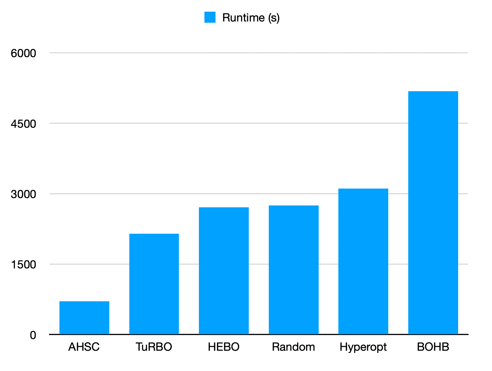
Figure 2: Algorithm runtimes on the vehicle dataset.

On a machine with an Intel Cascade Lake CPU with 4 vCPUs and 23GB RAM and no GPU, where we ran our NeurIPS Black-Box Optimization Challenge experiments, we measured the cost of computing the strong convexity over 15 runs with varying batch sizes. The median number of batches was 15.51 (442 samples), which took a median of 0.47 seconds. Therefore, it takes 0.03s/batch/config to compute the strong convexity. For example, the breast cancer dataset has 569 samples. Using the mean batch size in the hyper-parameter space of 130, that evaluates to 4.38 batches, which we expect to take $0.03\times 4.38\times 50=6.57$s to compute the strong convexity for 50 configurations.

The above experiments suggest that computing the strong convexity this way is computationally cheap, since we train for the full epochs only for the top 10 configurations. Figure 2 shows the runtimes for each algorithm on the vehicle dataset, on a machine with an RTX 2060 Super. Our approach requires between 13% to 33% of the runtime compared to other algorithms.

5 Conclusion and Future Work

In this paper, we developed a novel white-box hyper-parameter optimization algorithm that, after some cheap computation, requires only 10 full runs to find a good configuration. We demonstrated our results on 12 tabular and two image datasets.

It has not escaped our attention that this method does not allow the user to specify a preference for evaluation metrics such as recall or precision. We leave this as future work. In particular, we exploit the fact that the Pareto frontier is a subset of the convex hull of the hyper-parameter performance scores. To find configurations that do well on some metric, we traverse the Pareto frontier and compute quantized convex combinations of adjacent points and also test them. This is similar to the approach of Ammar (2004). However, this approach adds additional computational cost.

Our hyper-parameter optimization method has two key limitations: first, it is limited to learners for which a loss function can be defined. In some cases such as Naive Bayes, a surrogate such as the negative log-likelihood can be used, for which the strong convexity can be computed. Even in cases where the loss is not twice-differentiable, one can use a finite difference approximation to compute the Hessian (see Nocedal and Wright (1999)):

$$\frac{\partial^{2}f}{\partial x_{i}\partial x_{j}}(x)\approx\frac{1}{\epsilon^{2}}\left(f(x+\epsilon e_{i}+\epsilon e_{j})-f(x+\epsilon e_{i})-f(x+\epsilon e_{j})+f(x)\right)$$

where the error is $\mathcal{O}(\epsilon)$. The second, potentially more important limitation is that the strong convexity cannot be compared across learners, especially if different losses are used. For example, while algorithms such as TPE can be used on hyper-parameter spaces with multiple classes of learners, our approach cannot: the entire hyper-parameter space must have comparable strong convexity values, for which the same class of learners (such as neural networks, Naive Bayes, logistic regression, etc.) must be used. However, this can be resolved by using the same loss function across learning algorithms. For example, a negative log-likelihood ratio loss has been proposed for neural classifiers Yao et al. (2020), which is compatible with other learners.

Appendix A Related Work

Hyper-parameter optimization. There is significant prior work in hyper-parameter optimization Agrawal et al. [2019], Cowen-Rivers et al. [2022], Li et al. [2017], Bergstra et al. [2011], Bergstra and Bengio [2012], Falkner et al. [2018], Eriksson et al. [2019], Ansel et al. [2014b]. Indeed, as learning systems become more intricate, it is crucial that we eke out the most performance. However, this is a non-trivial problem, as evidenced by the long line of research in this direction.

The simplest form of hyper-parameter search is random search, which tries $n$ randomly chosen hyper-parameter configurations. Opentuner Ansel et al. [2014a] is a multi-armed bandit meta-technique with a sliding window that incorporates an exploration/exploitation trade-off based on the number of times a specific technique is used. It combines DE, a greedy bandit mutation technique, and hill-climbing methods.

Bayesian Optimization (BO) has emerged as the most popular technique for HPO. Bergstra et al. [2011] propose the Tree of Parzen Estimators (TPE) algorithm. Rather than model $p(y|x)$, TPE models $p(x|y)$ as

$$p(x|y)=\begin{cases}l(x)&y<y^{*}\\ g(x)&y\geq y^{*}\end{cases}$$

where $y^{*}$ is chosen so that $p(y<y^{*})=\gamma$ for some quantile $\gamma$. The functions $l(x)$ and $g(x)$ are kernel density estimates. TPE optimizes the EI, which they show is equivalent to maximizing $l(x)/g(x)$. Snoek et al. [2012] use Gaussian Process (GP) models as the surrogate function in Bayesian optimization. They use Expected Improvement (EI) as the acquisition function. Similarly, Hernández-Lobato et al. [2014] use predictive entropy search (PES) as the acquisition function. Swersky et al. [2014] exploit iterative training procedures in their Bayesian optimization framework, which they call freeze-thaw Bayesian optimization. Snoek et al. [2015] use neural networks for modeling distributions over functions that yields an approach that scales linearly over data size (rather than cubically as in GP-based Bayesian optimization). BOHB Falkner et al. [2018] combines the BO-based TPE with HyperBand Li et al. [2017], replacing the initial random configurations with a model-based search. Notably, BOHB uses a single multi-dimensional KDE instead of hierarchical single-dimensional KDEs used by TPE. The authors of HEBO Cowen-Rivers et al. [2022] note that (i) even simple HPO problems can be non-stationary and heteroscedastic (ii) different acquisition functions can conflict. To tackle the former, they use the Box-Cox Box and Cox [1964] and Yeo-Johnson Yeo and Johnson [2000] output transformations and the Kumaraswamy Kumaraswamy [1980] input transformation. It also uses NSGA-II to optimize a multi-objective acquisition function. TuRBO Dou et al. [2023] assumes the hyper-parameter to performance mapping is Lipschitz, and generates pseudo-points to improve convergence of vanilla BO. It also uses an ensemble of learners to predict performance, and if the prediction is poor, uses it to instead update the GP model. Finally, we mention PriorBand Mallik et al. [2023], which incorporates an expert’s prior beliefs about good configurations, but maintains good performance even if that prior is bad.

We defer to Feurer and Hutter [2019] and Bischl et al. [2023] for recent reviews on hyper-parameter optimization techniques. There is also a long line of work studying neural architecture search, which aims to find optimal architectures for a dataset. We refer the reader to White et al. [2023] for a comprehensive review of the field.

Several benchmarks have been proposed for hyper-parameter optimization: notable ones include YAHPO Gym Pfisterer et al. [2022], HPO-B Arango et al. [2021], and HPOBench Eggensperger et al. [2021].

Flat minima and generalization. The idea of flat minima was first studied by Hochreiter and Schmidhuber [1994]. In particular, they define “flat minima” as large connected regions where the weights are $\epsilon-$optimal. Hochreiter and Schmidhuber [1997] intuit that because sharper minima require higher precision, flatter minima require less bits to describe. They use this intuition to show that flat minima correspond to minimizing the number of bits required to describe the weights of a neural network. This notion of minimum description length (MDL) Rissanen [1983], Grünwald [2007] was also exploited early on by Hinton and Van Camp [1993]. Flat minima were revisited by Chaudhari et al. [2019], who noted that minima with low generalization error have a large proportion of their eigenvalues close to zero. They then construct a modified Gibbs distribution corresponding to an energy landscape $f$, and minimize the negative local entropy of this modified distribution, and approximate the gradient via stochastic gradient Langevin dynamics (SGLD) Welling and Teh [2011]. However, their assumptions were, admittedly unrealistic. Keskar et al. [2016] show that when using large batch sizes, optimizers converge to sharp minima, which are characterized by many large positive eigenvalues of the Hessian. Further, they define the notion of sharpness as a generalization measure as the robustness to adversarial perturbations in the parameter space:

$$\zeta(\boldsymbol{w};\epsilon)=\frac{\max\limits_{\left\lvert\boldsymbol{v}\right\rvert\leq\epsilon(\left\lvert\boldsymbol{w}\right\rvert+1)}f(\boldsymbol{w}+\boldsymbol{v})-f(\boldsymbol{w})}{1+f(\boldsymbol{w})}$$ (6)

and compute this using 10 iterations of L-BFGS-B Byrd et al. [1995] with $\epsilon=\{10^{-3},5\cdot 10^{-4}\}$. In particular, the above is closely related to the largest eigenvalue of $\nabla^{2}f(\boldsymbol{w})$. This notion of sharpness was also endorsed by Jiang et al. [2019], who performed a large-scale study of many complexity measures on two datasets, with 2,187 convolutional networks. In particular, they endorse the following metrics for generalization: (i) variance of gradients (ii) squared ratio of magnitude of parameters to magnitude of perturbation, à la Keskar et al. [2016] (iii) path norm Neyshabur et al. [2017] (iv) VC-dimension (inversely correlated).

A line of work in physics Baldassi et al. [2015, 2016] showed that in the discrete weight scenario (a much more difficult problem), isolated minima were rare, but there existed accessible, dense regions of subdominant minima, and that these were robust to perturbations and generalized better. These authors devised algorithms explicitly designed to search for nonisolated minima. In the continuous weight space, nonisolated minima correspond to flat minima. Dziugaite and Roy [2017] obtain nonvacuous generalization bounds for deep overparameterized neural networks using the PAC-Bayes framework McAllester [1999]. Neyshabur et al. [2014] showed that increasing the number of hidden units (which in turn, increases the number of trainable parameters) can lead to a decrease in generalization error with the same training error. Neyshabur et al. [2017] showed that sharpness as computed by (6) is not sufficient to capture the generalization behavior (but noting that “combined with the norm, sharpness does seem to provide a capacity measure”), and advocate for expected sharpness in the PAC-Bayesian framework, similar to Dziugaite and Roy [2017]. They show that plots of expected sharpness versus KL divergence in PAC-Bayes bounds for varying dataset sizes capture generalization well. Li et al. [2018] showed that the sharpness of the loss surface correlates well with the generalization error. In their seminal paper, Jastrzebski et al. [2017] showed that SGD is a Euler-Maruyama discretization of a stochastic differential equation whose dynamics are influenced by the ratio of learning rate to batch size (which they call “stochastic noise”), and that SGD finds wider minima with higher stochastic noise levels than sharper minima. Wu and Su [2023] study the flat minima hypothesis through the lens of dynamical stability, and show that SGD will escape from overly sharp (measured by the Frobenius norm of the Hessian), low-loss areas exponentially fast. We note that they use the associate empirical Fisher matrix (AEFM) as an approximation for the Hessian, which holds for low empirical risk (and converges to the Hessian, see Kunstner et al. [2019]).

In search of flatter loss surfaces, Seong et al. [2018] propose the use of non-monotonic learning rate schedules. They advocate for large learning rates, which enable the optimization algorithm to escape sharp minima, and descend into flatter minima. The seminal works of Dauphin et al. [2014] and Choromanska et al. [2015] showed both theoretically and empirically that local minima are more likely to be located close to the global minimum. In particular, Dauphin et al. [2014] showed using the perspectives of random matrix theory (via the eigenvalue distribution of Gaussian random matrices Wigner [1958]), statistical physics (via the analysis of critical points in Gaussian fields by Bray and Dean [2007]), and neural network theory Saxe et al. [2013] that saddle points are exponentially less likely than local minima.

Most recently, Wen et al. [2023] showed that sharpness is neither necessary, nor sufficient for generalization, by studying some simple architectures, showing that generalization depends on the data distribution as well as the architecture; for example, merely adding a bias to a 2-layer MLP makes generalization impossible for the XOR dataset.

Of course, it is not possible to discuss generalization in deep learning without discussing the results of Zhang et al. [2021], who showed that deep learners can fit with zero training error on random labels using an architecture that generalizes well when fit to the correct labels. Bartlett et al. [2019] and Harvey et al. [2017] found that the VC-dimension for deep ReLU networks is $\mathcal{O}(WL\log W)$ and $\Theta(WU)$ respectively, where $W$ is the number of parameters, $L$ the number of layers, and $U$ the number of units. Hardt et al. [2016] show that stochastic gradient methods are uniformly stable, which implies generalization in expectation.

Appendix B Background

Definition 1 (Fenchel conjugate).

The Fenchel conjugate, $f^{*}:\mathcal{X}\to\mathbb{R}^{*}$ for a convex function $f:\mathcal{X}\to\mathbb{R}^{*}$ is defined as $f^{*}(y)=\sup\limits_{x\in\mathcal{X}}\langle x,y\rangle-f(x)$

Definition 2 (Dual norm).

Given a norm $\lVert\cdot\rVert$ on $\mathcal{X}$, the dual norm $\lVert\cdot\rVert_{*}$ is defined as

$$\lVert y\rVert_{*}=\sup\{\langle x,y\rangle:\lVert x\rVert\leq 1\}$$

Note that the Fenchel conjugate of $\frac{1}{2}\lVert x\rVert$ is $\frac{1}{2}\lVert y\rVert_{*}$.

Definition 3 (Strong convexity).

A function $f:\mathcal{X}\to\mathbb{R}^{*}$ is $\mu-$strongly convex with respect to $\lVert\cdot\rVert$ if $\forall x,y$ in the relative interior of $\text{dom }f$ and $\alpha\in(0,1)$,

$$f(\alpha x+(1-\alpha)y)\leq\alpha f(x)+(1-\alpha)f(y)-\frac{1}{2}\mu\alpha(1-\alpha)\lVert x-y\rVert^{2}$$

Definition 4 (Smoothness).

A function $f:\mathcal{X}\to\mathbb{R}$ is $\beta-$smooth with respect to $\lVert\cdot\rVert$ if $f\in C^{1}$ and if $\forall x,y\in\text{dom }f$,

$$f(x+y)\leq f(x)+\langle\nabla f(x),y\rangle+\frac{1}{2}\beta\lVert y\rVert^{2}$$

Appendix C Auxiliary Proofs

Lemma 3.

Let $f:\mathbb{R}^{d}\to\mathbb{R}$ be a differentiable function. Then, $\mu-$strong convexity implies:

1. (Polyak-Łojasiewicz (PL) inequality)

   $$\frac{1}{2}\left\lVert\nabla f(x)\right\rVert^{2}\geq\mu(f(x)-f(x^{*}))$$

2. $$\left\lVert\nabla f(x)-\nabla f(y)\right\rVert\geq\mu\left\lVert x-y\right\rVert$$

3. $$\left(\nabla f(x)-\nabla f(y)\right)^{T}(x-y)\leq\frac{1}{\mu}\left\lVert\nabla f(x)-\nabla f(y)\right\rVert^{2}$$

Proof.

1. Strong convexity implies

   $$f(y)\geq f(x)+\nabla f(x)^{T}(y-x)+\frac{\mu}{2}\left\lVert y-x\right\rVert^{2}$$

   Minimizing with respect to $y$ yields the result.

2. Strong convexity gives us:

   $$\left(\nabla f(x)-\nabla f(y)\right)^{T}(x-y)\geq\mu\left\lVert x-y\right\rVert^{2}$$ (7)

   Applying Cauchy-Schwarz inequality gives us:

   where the last step comes from (7).

3. Set $\phi_{x}(z)=f(z)-\nabla f(x)^{T}z$. It is easy to see that $\phi_{x}$ is also $\mu-$strongly convex. Applying the Polyak-Łojasiewicz inequality to $\phi_{x}(z)$ with $z^{*}=x$,

   Swapping $x$ and $y$ in the above,

   Adding (iii) and (8) yields the result.

∎

Lemma 4.

If $f:\mathbb{R}^{n}\to\mathbb{R}$ is smooth and $\mu-$strongly convex, then

$$\frac{1}{2\mu}\left\lVert\nabla f(x)\right\rVert^{2}\geq f(x)-f(x^{*})\geq\frac{\mu}{2}\left\lVert x-x^{*}\right\rVert^{2}$$

Proof.

The first part is the Polyak-Łojasiewicz inequality. The second part follows from the definition of strong convexity and setting $y=x,x=x^{*}$ and using $f(x^{*})\geq\min\limits_{y}f(y)$. ∎

Theorem 2 (Smooth and strongly convex gradient descent).

Suppose $f:\mathbb{R}^{n}\to\mathbb{R}$ be $\beta-$smooth and $\mu-$strongly convex. Then with the gradient descent update rule

$$x_{k+1}=x_{k}-\frac{1}{\beta}\nabla f(x_{k})$$

where $\frac{1}{\beta}$ is the learning rate, we have

$$f(x_{k})-f(x^{*})\leq\left(1-\frac{\mu}{\beta}\right)^{k}(f(x_{0})-f(x^{*}))$$

Consequently, we require $\frac{\beta}{\mu}\log\frac{f(x_{0})-f(x^{*})}{\epsilon}$ iterations to find an $\epsilon-$optimal point.

Proof.

From the above results,

$$f(x_{k+1})\leq f(x_{k})-\frac{1}{2\beta}\left\lVert\nabla f(x_{k})\right\rVert^{2}$$

and Lemma 4 gives us

$$\left\lVert\nabla f(x_{k})\right\rVert^{2}\geq 2\mu(f(x_{k})-f(x^{*}))$$

Therefore,

$$f(x_{k+1})-f(x^{*}) \leq f(x_{k})-f(x^{*})-\frac{1}{2\beta}\left\lVert\nabla f(x_{k})\right\rVert^{2}$$

$$\leq f(x_{k})-f(x^{*})-\frac{\mu}{\beta}(f(x_{k})-f(x^{*}))$$

$$=\left(1-\frac{\mu}{\beta}\right)(f(x_{k})-f(x^{*}))$$

$$f(x_{k})-f(x^{*}) \leq\left(1-\frac{\mu}{\beta}\right)^{k}(f(x_{k})-f(x^{*}))$$

$$\leq\exp\left(-\frac{\mu k}{\beta}\right)(f(x_{0})-f(x^{*}))$$

Therefore we need $k=\frac{\beta}{\mu}\log\frac{f(x_{0})-f(x^{*})}{\epsilon}$ iterations for $\epsilon-$optimality. ∎

Note that strong convexity guarantees optimality. $\beta-$smoothness can only assure $\epsilon-$criticality. This implies the existence of global minima.

Strong convexity is a necessary condition for learnability, as along with $\beta-$smoothness, it can be shown that such problems are learnable Shalev-Shwartz and Ben-David [2014]. Additionally, strong convexity provides a quadratic lower bound on the growth of the loss function, which implies that the convexity condition will never be violated in the local domain of the function in the context of deep regression with regularization.

Theorem 3.

Suppose $f$ is a closed and convex function. Then $f$ is $\beta-$strongly convex with respect to a norm $\lVert\cdot\rVert$ iff $f^{*}$ is $\frac{1}{\beta}-$smooth with respect to the dual norm $\lVert\cdot\rVert_{*}$. That is, if $f^{*}$ is smooth, then $f$ is strongly convex.

Proof.

We defer the proofs to Shalev-Shwartz and Singer [2007], Lemma 15 ($1\Rightarrow 2$) and Kakade et al. [2009], Theorem 6 ($2\Rightarrow 1$).

∎

The above result has implications for the generalization bounds of various algorithms, such as lasso regression (which is a special case of the group lasso algorithm discussed in Kakade et al. [2009]), kernel learning, and online control. For a detailed exposition, we refer the reader to Kakade et al. [2009].

References

- Agrawal et al. [2019] Amritanshu Agrawal, Wei Fu, Di Chen, Xipeng Shen, and Tim Menzies. How to “dodge” complex software analytics. IEEE Transactions on Software Engineering, 47(10):2182–2194, 2019.
- Ammar [2004] Kareem Ammar. Multi-heuristic theory assessment with iterative selection. West Virginia University, 2004.
- Ansel et al. [2014a] Jason Ansel, Shoaib Kamil, Kalyan Veeramachaneni, Jonathan Ragan-Kelley, Jeffrey Bosboom, Una-May O’Reilly, and Saman Amarasinghe. Opentuner: An extensible framework for program autotuning. In Proceedings of the 23rd international conference on Parallel architectures and compilation, pages 303–316, 2014a.
- Ansel et al. [2014b] Jason Ansel, Shoaib Kamil, Kalyan Veeramachaneni, Jonathan Ragan-Kelley, Jeffrey Bosboom, Una-May O’Reilly, and Saman Amarasinghe. Opentuner: An extensible framework for program autotuning. In International Conference on Parallel Architectures and Compilation Techniques (PACT), Edmonton, Canada, Aug 2014b. URL http://groups.csail.mit.edu/commit/papers/2014/ansel-pact14-opentuner.pdf.
- Arango et al. [2021] Sebastian Pineda Arango, Hadi Samer Jomaa, Martin Wistuba, and Josif Grabocka. Hpo-b: A large-scale reproducible benchmark for black-box hpo based on openml. In Thirty-fifth Conference on Neural Information Processing Systems Datasets and Benchmarks Track (Round 2), 2021.
- Awad et al. [2021] Noor Awad, Neeratyoy Mallik, and Frank Hutter. Dehb: Evolutionary hyperband for scalable, robust and efficient hyperparameter optimization. arXiv preprint arXiv:2105.09821, 2021.
- Baldassi et al. [2015] Carlo Baldassi, Alessandro Ingrosso, Carlo Lucibello, Luca Saglietti, and Riccardo Zecchina. Subdominant dense clusters allow for simple learning and high computational performance in neural networks with discrete synapses. Physical review letters, 115(12):128101, 2015.
- Baldassi et al. [2016] Carlo Baldassi, Christian Borgs, Jennifer T Chayes, Alessandro Ingrosso, Carlo Lucibello, Luca Saglietti, and Riccardo Zecchina. Unreasonable effectiveness of learning neural networks: From accessible states and robust ensembles to basic algorithmic schemes. Proceedings of the National Academy of Sciences, 113(48):E7655–E7662, 2016.
- Bartlett et al. [2019] Peter L Bartlett, Nick Harvey, Christopher Liaw, and Abbas Mehrabian. Nearly-tight vc-dimension and pseudodimension bounds for piecewise linear neural networks. The Journal of Machine Learning Research, 20(1):2285–2301, 2019.
- Bergstra and Bengio [2012] James Bergstra and Yoshua Bengio. Random search for hyper-parameter optimization. Journal of machine learning research, 13(2), 2012.
- Bergstra et al. [2011] James Bergstra, Rémi Bardenet, Yoshua Bengio, and Balázs Kégl. Algorithms for hyper-parameter optimization. Advances in neural information processing systems, 24, 2011.
- Bergstra et al. [2013] James Bergstra, Daniel Yamins, and David Daniel Cox. Making a science of model search: Hyperparameter optimization in hundreds of dimensions for vision architectures. 2013.
- Bischl et al. [2023] Bernd Bischl, Martin Binder, Michel Lang, Tobias Pielok, Jakob Richter, Stefan Coors, Janek Thomas, Theresa Ullmann, Marc Becker, Anne-Laure Boulesteix, et al. Hyperparameter optimization: Foundations, algorithms, best practices, and open challenges. Wiley Interdisciplinary Reviews: Data Mining and Knowledge Discovery, 13(2):e1484, 2023.
- Box and Cox [1964] George EP Box and David R Cox. An analysis of transformations. Journal of the Royal Statistical Society Series B: Statistical Methodology, 26(2):211–243, 1964.
- Bray and Dean [2007] Alan J Bray and David S Dean. Statistics of critical points of gaussian fields on large-dimensional spaces. Physical review letters, 98(15):150201, 2007.
- Byrd et al. [1995] Richard H Byrd, Peihuang Lu, Jorge Nocedal, and Ciyou Zhu. A limited memory algorithm for bound constrained optimization. SIAM Journal on scientific computing, 16(5):1190–1208, 1995.
- Chaudhari et al. [2019] Pratik Chaudhari, Anna Choromanska, Stefano Soatto, Yann LeCun, Carlo Baldassi, Christian Borgs, Jennifer Chayes, Levent Sagun, and Riccardo Zecchina. Entropy-sgd: Biasing gradient descent into wide valleys. Journal of Statistical Mechanics: Theory and Experiment, 2019(12):124018, 2019.
- Choromanska et al. [2015] Anna Choromanska, Mikael Henaff, Michael Mathieu, Gérard Ben Arous, and Yann LeCun. The loss surfaces of multilayer networks. In Artificial intelligence and statistics, pages 192–204. PMLR, 2015.
- Cowen-Rivers et al. [2022] Alexander I Cowen-Rivers, Wenlong Lyu, Rasul Tutunov, Zhi Wang, Antoine Grosnit, Ryan Rhys Griffiths, Alexandre Max Maraval, Hao Jianye, Jun Wang, Jan Peters, et al. Hebo: pushing the limits of sample-efficient hyper-parameter optimisation. Journal of Artificial Intelligence Research, 74:1269–1349, 2022.
- Dauphin et al. [2014] Yann N Dauphin, Razvan Pascanu, Caglar Gulcehre, Kyunghyun Cho, Surya Ganguli, and Yoshua Bengio. Identifying and attacking the saddle point problem in high-dimensional non-convex optimization. Advances in neural information processing systems, 27, 2014.
- Dinh et al. [2017] Laurent Dinh, Razvan Pascanu, Samy Bengio, and Yoshua Bengio. Sharp minima can generalize for deep nets. In International Conference on Machine Learning, pages 1019–1028. PMLR, 2017.
- Dou et al. [2023] Hui Dou, Lei Zhang, Yiwen Zhang, Pengfei Chen, and Zibin Zheng. Turbo: A cost-efficient configuration-based auto-tuning approach for cluster-based big data frameworks. Journal of Parallel and Distributed Computing, 177:89–105, 2023.
- Duchi [2023] John Duchi. Lecture notes on statistics and information theory. https://web.stanford.edu/class/stats311/lecture-notes.pdf, 2023.
- Dziugaite and Roy [2017] Gintare Karolina Dziugaite and Daniel M Roy. Computing nonvacuous generalization bounds for deep (stochastic) neural networks with many more parameters than training data. arXiv preprint arXiv:1703.11008, 2017.
- Eggensperger et al. [2021] Katharina Eggensperger, Philipp Müller, Neeratyoy Mallik, Matthias Feurer, Rene Sass, Aaron Klein, Noor Awad, Marius Lindauer, and Frank Hutter. Hpobench: A collection of reproducible multi-fidelity benchmark problems for hpo. In Thirty-fifth Conference on Neural Information Processing Systems Datasets and Benchmarks Track (Round 2), 2021.
- Eriksson et al. [2019] David Eriksson, Michael Pearce, Jacob Gardner, Ryan D Turner, and Matthias Poloczek. Scalable global optimization via local bayesian optimization. Advances in neural information processing systems, 32, 2019.
- Falkner et al. [2018] Stefan Falkner, Aaron Klein, and Frank Hutter. Bohb: Robust and efficient hyperparameter optimization at scale. In International Conference on Machine Learning, pages 1437–1446. PMLR, 2018.
- Farcomeni [2008] Alessio Farcomeni. A review of modern multiple hypothesis testing, with particular attention to the false discovery proportion. Statistical methods in medical research, 17(4):347–388, 2008.
- Feurer and Hutter [2019] Matthias Feurer and Frank Hutter. Hyperparameter optimization. In Automated machine learning, pages 3–33. Springer, Cham, 2019.
- Grünwald [2007] Peter D Grünwald. The minimum description length principle. MIT press, 2007.
- Hardt et al. [2016] Moritz Hardt, Ben Recht, and Yoram Singer. Train faster, generalize better: Stability of stochastic gradient descent. In International conference on machine learning, pages 1225–1234. PMLR, 2016.
- Harvey et al. [2017] Nick Harvey, Christopher Liaw, and Abbas Mehrabian. Nearly-tight vc-dimension bounds for piecewise linear neural networks. In Conference on learning theory, pages 1064–1068. PMLR, 2017.
- Hernández-Lobato et al. [2014] José Miguel Hernández-Lobato, Matthew W Hoffman, and Zoubin Ghahramani. Predictive entropy search for efficient global optimization of black-box functions. Advances in neural information processing systems, 27, 2014.
- Hinton and Van Camp [1993] Geoffrey E Hinton and Drew Van Camp. Keeping the neural networks simple by minimizing the description length of the weights. In Proceedings of the sixth annual conference on Computational learning theory, pages 5–13, 1993.
- Hochreiter and Schmidhuber [1994] Sepp Hochreiter and Jürgen Schmidhuber. Simplifying neural nets by discovering flat minima. Advances in neural information processing systems, 7, 1994.
- Hochreiter and Schmidhuber [1997] Sepp Hochreiter and Jürgen Schmidhuber. Flat minima. Neural computation, 9(1):1–42, 1997.
- Jastrzebski et al. [2017] Stanisław Jastrzebski, Zachary Kenton, Devansh Arpit, Nicolas Ballas, Asja Fischer, Yoshua Bengio, and Amos Storkey. Three factors influencing minima in sgd. arXiv preprint arXiv:1711.04623, 2017.
- Jiang et al. [2019] Yiding Jiang, Behnam Neyshabur, Hossein Mobahi, Dilip Krishnan, and Samy Bengio. Fantastic generalization measures and where to find them. arXiv preprint arXiv:1912.02178, 2019.
- Kakade et al. [2009] Sham Kakade, Shai Shalev-Shwartz, Ambuj Tewari, et al. On the duality of strong convexity and strong smoothness: Learning applications and matrix regularization. Unpublished Manuscript, http://ttic. uchicago. edu/shai/papers/KakadeShalevTewari09. pdf, 2(1):35, 2009.
- Keskar et al. [2016] Nitish Shirish Keskar, Dheevatsa Mudigere, Jorge Nocedal, Mikhail Smelyanskiy, and Ping Tak Peter Tang. On large-batch training for deep learning: Generalization gap and sharp minima. arXiv preprint arXiv:1609.04836, 2016.
- Kingma and Ba [2014] Diederik P Kingma and Jimmy Ba. Adam: A method for stochastic optimization. arXiv preprint arXiv:1412.6980, 2014.
- Kumaraswamy [1980] Ponnambalam Kumaraswamy. A generalized probability density function for double-bounded random processes. Journal of hydrology, 46(1-2):79–88, 1980.
- Kunstner et al. [2019] Frederik Kunstner, Philipp Hennig, and Lukas Balles. Limitations of the empirical fisher approximation for natural gradient descent. Advances in neural information processing systems, 32, 2019.
- Lacoste et al. [2019] Alexandre Lacoste, Alexandra Luccioni, Victor Schmidt, and Thomas Dandres. Quantifying the carbon emissions of machine learning. arXiv preprint arXiv:1910.09700, 2019.
- LeCun [1998] Yann LeCun. The mnist database of handwritten digits. http://yann. lecun. com/exdb/mnist/, 1998.
- Li et al. [2018] Hao Li, Zheng Xu, Gavin Taylor, Christoph Studer, and Tom Goldstein. Visualizing the loss landscape of neural nets. Advances in neural information processing systems, 31, 2018.
- Li et al. [2017] Lisha Li, Kevin Jamieson, Giulia DeSalvo, Afshin Rostamizadeh, and Ameet Talwalkar. Hyperband: A novel bandit-based approach to hyperparameter optimization. The Journal of Machine Learning Research, 18(1):6765–6816, 2017.
- Majumder et al. [2018] Suvodeep Majumder, Nikhila Balaji, Katie Brey, Wei Fu, and Tim Menzies. 500+ times faster than deep learning. In Proceedings of the 15th International Conference on Mining Software Repositories. ACM, 2018.
- Mallik et al. [2023] Neeratyoy Mallik, Edward Bergman, Carl Hvarfner, Danny Stoll, Maciej Janowski, Marius Lindauer, Luigi Nardi, and Frank Hutter. Priorband: Practical hyperparameter optimization in the age of deep learning. arXiv preprint arXiv:2306.12370, 2023.
- Mann and Whitney [1947] Henry B Mann and Donald R Whitney. On a test of whether one of two random variables is stochastically larger than the other. The annals of mathematical statistics, pages 50–60, 1947.
- McAllester [1999] David A McAllester. Pac-bayesian model averaging. In Proceedings of the twelfth annual conference on Computational learning theory, pages 164–170, 1999.
- Netzer et al. [2011] Yuval Netzer, Tao Wang, Adam Coates, Alessandro Bissacco, Bo Wu, and Andrew Y Ng. Reading digits in natural images with unsupervised feature learning. 2011.
- Neyshabur et al. [2014] Behnam Neyshabur, Ryota Tomioka, and Nathan Srebro. In search of the real inductive bias: On the role of implicit regularization in deep learning. arXiv preprint arXiv:1412.6614, 2014.
- Neyshabur et al. [2017] Behnam Neyshabur, Srinadh Bhojanapalli, David McAllester, and Nati Srebro. Exploring generalization in deep learning. Advances in neural information processing systems, 30, 2017.
- Nocedal and Wright [1999] Jorge Nocedal and Stephen J Wright. Numerical optimization. Springer, 1999.
- Pfisterer et al. [2022] Florian Pfisterer, Lennart Schneider, Julia Moosbauer, Martin Binder, and Bernd Bischl. Yahpo gym-an efficient multi-objective multi-fidelity benchmark for hyperparameter optimization. In International Conference on Automated Machine Learning, pages 3–1. PMLR, 2022.
- Rissanen [1983] Jorma Rissanen. A universal prior for integers and estimation by minimum description length. The Annals of statistics, 11(2):416–431, 1983.
- Santurkar et al. [2018] Shibani Santurkar, Dimitris Tsipras, Andrew Ilyas, and Aleksander Madry. How does batch normalization help optimization? Advances in neural information processing systems, 31, 2018.
- Saxe et al. [2013] Andrew M Saxe, James L McClelland, and Surya Ganguli. Exact solutions to the nonlinear dynamics of learning in deep linear neural networks. arXiv preprint arXiv:1312.6120, 2013.
- Seong et al. [2018] Sihyeon Seong, Yegang Lee, Youngwook Kee, Dongyoon Han, and Junmo Kim. Towards flatter loss surface via nonmonotonic learning rate scheduling. In UAI, pages 1020–1030, 2018.
- Shalev-Shwartz and Ben-David [2014] Shai Shalev-Shwartz and Shai Ben-David. Understanding machine learning: From theory to algorithms. Cambridge university press, 2014.
- Shalev-Shwartz and Singer [2007] Shai Shalev-Shwartz and Yoram Singer. A primal-dual perspective of online learning algorithms. Machine Learning, 69:115–142, 2007.
- Smith [2018] Leslie N Smith. A disciplined approach to neural network hyper-parameters: Part 1–learning rate, batch size, momentum, and weight decay. arXiv preprint arXiv:1803.09820, 2018.
- Snoek et al. [2012] Jasper Snoek, Hugo Larochelle, and Ryan P Adams. Practical bayesian optimization of machine learning algorithms. Advances in neural information processing systems, 25, 2012.
- Snoek et al. [2015] Jasper Snoek, Oren Rippel, Kevin Swersky, Ryan Kiros, Nadathur Satish, Narayanan Sundaram, Mostofa Patwary, Mr Prabhat, and Ryan Adams. Scalable bayesian optimization using deep neural networks. In International conference on machine learning, pages 2171–2180. PMLR, 2015.
- Swersky et al. [2014] Kevin Swersky, Jasper Snoek, and Ryan Prescott Adams. Freeze-thaw bayesian optimization. arXiv preprint arXiv:1406.3896, 2014.
- Tantithamthavorn et al. [2016] Chakkrit Tantithamthavorn, Shane McIntosh, Ahmed E. Hassan, and Kenichi Matsumoto. Automated parameter optimization of classification techniques for defect prediction models. In 2016 IEEE/ACM 38th International Conference on Software Engineering (ICSE), pages 321–332, 2016. doi: 10.1145/2884781.2884857.
- Tran et al. [2020] Ngoc Tran, Jean-Guy Schneider, Ingo Weber, and A Kai Qin. Hyper-parameter optimization in classification: To-do or not-to-do. Pattern Recognition, 103:107245, 2020.
- Welling and Teh [2011] Max Welling and Yee W Teh. Bayesian learning via stochastic gradient langevin dynamics. In Proceedings of the 28th international conference on machine learning (ICML-11), pages 681–688, 2011.
- Wen et al. [2023] Kaiyue Wen, Zhiyuan Li, and Tengyu Ma. Sharpness minimization algorithms do not only minimize sharpness to achieve better generalization. In Thirty-seventh Conference on Neural Information Processing Systems, 2023.
- White et al. [2023] Colin White, Mahmoud Safari, Rhea Sukthanker, Binxin Ru, Thomas Elsken, Arber Zela, Debadeepta Dey, and Frank Hutter. Neural architecture search: Insights from 1000 papers. arXiv preprint arXiv:2301.08727, 2023.
- Wigner [1958] Eugene P Wigner. On the distribution of the roots of certain symmetric matrices. Annals of Mathematics, 67(2):325–327, 1958.
- Wu and Su [2023] Lei Wu and Weijie J Su. The implicit regularization of dynamical stability in stochastic gradient descent. arXiv preprint arXiv:2305.17490, 2023.
- Yao et al. [2020] Hengshuai Yao, Dong-lai Zhu, Bei Jiang, and Peng Yu. Negative log likelihood ratio loss for deep neural network classification. In Proceedings of the Future Technologies Conference (FTC) 2019: Volume 1, pages 276–282. Springer, 2020.
- Yeo and Johnson [2000] In-Kwon Yeo and Richard A Johnson. A new family of power transformations to improve normality or symmetry. Biometrika, 87(4):954–959, 2000.
- Zhang et al. [2021] Chiyuan Zhang, Samy Bengio, Moritz Hardt, Benjamin Recht, and Oriol Vinyals. Understanding deep learning (still) requires rethinking generalization. Communications of the ACM, 64(3):107–115, 2021.