A Sober Look at LLMs for Material Discovery:
Are They Actually Good for Bayesian Optimization Over Molecules?

Abstract

Automation is one of the cornerstones of contemporary material discovery. Bayesian optimization (BO) is an essential part of such workflows, enabling scientists to leverage prior domain knowledge into efficient exploration of a large molecular space. While such prior knowledge can take many forms, there has been significant fanfare around the ancillary scientific knowledge encapsulated in large language models (LLMs). However, existing work thus far has only explored LLMs for heuristic materials searches. Indeed, recent work obtains the uncertainty estimate—an integral part of BO—from point-estimated, non-Bayesian LLMs. In this work, we study the question of whether LLMs are actually useful to accelerate principled Bayesian optimization in the molecular space. We take a sober, dispassionate stance in answering this question. This is done by carefully (i) viewing LLMs as fixed feature extractors for standard but principled BO surrogate models and by (ii) leveraging parameter-efficient finetuning methods and Bayesian neural networks to obtain the posterior of the LLM surrogate. Our extensive experiments with real-world chemistry problems show that LLMs can be useful for BO over molecules, but only if they have been pretrained or finetuned with domain-specific data.

[1] $\triangleright$ #1 [1]$\triangleright$ #1

1 Introduction

Figure 1: LLMs seem to “understand” chemistry. However, they often produce completely wrong answers while sounding very convincing. Both APIs were accessed on 2024-01-07.

Material discovery describes the inherently laborious, iterative process of designing materials candidates, preparing them experimentally, testing their properties, and eventually updating the initial design hypothesis (de Regt, 2020; Greenaway et al., 2023). While human researchers have largely driven this process for the last century, there is demand for more efficient automated methods in the face of pressing societal challenges related to health care, nutrition, or clean energy (Tom et al., 2024). Major challenges associated with the discovery process are the complex and black box-like mapping between a material’s structure and its properties, as well as the vastness of the design space (Wang et al., 2023).

(a) Fixed-feature LLM surrogate

(b) Adaptive-feature LLM surrogate

Figure 2: The surrogates we consider in this work. “PEFT” refers to parameter efficient finetuning which adds few trainable weights $\bm{\omega}$ to the transformer. Grey means the weights are frozen and thus act as conditioning variables in the posterior over the surrogate $g_{t}$. Green means the weights are trained in a Bayesian manner (e.g., to obtain $p({\bm{w}},\bm{\omega}\mid\mathcal{D}_{t})$) and then marginalized to obtain the posterior predictive distribution over $g_{t}$ (e.g., $\iint p(g_{t}(\,\cdot\,)\mid{\bm{w}},\bm{\omega};{\bm{W}}_{*})\,p({\bm{w}},\bm{\omega}\mid\mathcal{D}_{t})\,d{\bm{w}}\,d\bm{\omega}$). Note that both models are principled Bayesian surrogates, in contrast to the in-context learning frameworks considered by prior works on BO with LLMs (Ramos et al., 2023; Anonymous, 2023).

To address the aforementioned problems, Bayesian optimization (BO; Močkus, 1975) has been increasingly used in chemistry (Griffiths et al., 2023; Hickman et al., 2023). Key components of successful BO include its priors (informative priors imply efficient posterior inference with limited data) and its probabilistic surrogate models (e.g. via Gaussian processes (Rasmussen & Williams, 2005; Snoek et al., 2012) or Bayesian neural networks (Kim et al., 2022; Li et al., 2023; Kristiadi et al., 2023)). The probabilistic formulation of BO is useful since optimizing a black-box function is an inherently uncertain problem—we do not know a priori the form of that function and our approximation of it might be imprecise. Uncertainty-aware surrogate models are thus useful to quantify the inherent uncertainty surrounding the optimization landscape, allowing for principled approaches to the exploration-exploitation tradeoff (Garnett, 2023).

However good priors needed for constructing accurate uncertainty estimates are hard to define analytically. Implicit priors, often obtained through pretrained feature extractors (Chithrananda et al., 2020; Ross et al., 2022), have thus been used instead. Recently, large language models (LLMs) have become very popular in many domains that are traditionally rather disconnected from natural language processing, such as in biology (Vig et al., 2021), education (Kasneci et al., 2023), law (Chalkidis et al., 2020), and chemistry (Maik Jablonka et al., 2023; Guo et al., 2023; Jablonka et al., 2023, etc.). On the other hand, recent works have warned that LLMs might not necessarily understand things, but simply act as very expensive “stochastic parrots” (Bender et al., 2021), see Figure 1 for example. Nevertheless, due to the apparent capabilities of LLMs, some recent works have leveraged off-the-shelf LLMs such as GPT-4 (OpenAI, 2023) for BO over molecules (Ramos et al., 2023) and for hyperparameter tuning (Anonymous, 2023). However, their uncertainty estimates are obtained only through heuristics, such as from the softmax probabilities of the generated answer tokens, coming from point-estimated non-Bayesian LLMs. These non-Bayesian uncertainties thus might not be optimal for the exploration-exploitation tradeoff that is so crucial for BO (Garnett, 2023).

In this work, we take a dispassionate look at LLMs for BO over molecules. We do so by carefully constructing and studying two kinds of surrogate models that are amenable to a principled Bayesian treatment, see Figure 2. First, we treat the LLM as a fixed feature extractor and find out whether its features are already useful as they are for BO over molecules. Second, we attempt to answer whether the “stochastic parrot” can be “taught”—via parameter-efficient fine-tuning methods (e.g., Houlsby et al., 2019; Li & Liang, 2021; Hu et al., 2022) and the Laplace approximation (MacKay, 1992a; Daxberger et al., 2021)—to perform efficient Bayesian exploration in the molecular space.

In sum, our contribution is four-fold:

1. We study the out-of-the-box usefulness of pretrained LLMs for material discovery by using their last embeddings in BO.

2. We study whether finetuning through PEFT and then applying approximate Bayesian inference over it is worth the effort in terms of the BO performance.

3. We provide an easy-to-use software library for principled BO on discrete space with LLMs: https://github.com/wiseodd/lapeft-bayesopt.

4. Through our extensive experiments ($8$ real-world chemistry problems, $8$ recent LLMs—including LLAMA-2—and non-LLM based features), we provide insights on whether, when, and how “stochastic parrots” can be useful to drive better scientific discovery.

Limitations

Our focus in this work is to study LLMs for discrete BO on a predetermined set of molecules, as usually done in real-world chemistry labs (Strieth-Kalthoff et al., 2023, etc.). We leave the study of BO on continuous space with principled LLM-based Bayesian surrogates as future work. Finally, we focus only on chemistry, although our experiments can also be done for other domains.

2 Preliminaries

Here, we introduce key concepts in Bayesian optimization, Bayesian neural networks, and large language models.

2.1 Bayesian optimization

Suppose $f:\mathcal{X}\to\mathcal{Y}$ is a function that is not analytically tractable and/or very expensive to evaluate. We would like (without loss of generality) to find ${\bm{x}}_{*}=\operatorname*{arg\,max}_{{\bm{x}}\in\mathcal{X}}f({\bm{x}})$. For example, we might want to find a new drug ${\bm{x}}$ in the space of all drugs $\mathcal{X}$ that has high efficacy over the population $f({\bm{x}})$. An increasingly common way to approach this problem is to perform Bayesian optimization (BO). The key components of BO are: (i) a surrogate function $g$ that tractably approximate $f$; (ii) a prior belief and a likelihood (and hence a posterior) over $g$; and (iii) an acquisition function $\alpha:\mathcal{X}\to\mathbb{R}$ that implicitly defines a policy for choosing which ${\bm{x}}\in\mathcal{X}$ to evaluate $f$ at. The expressiveness of $g$ dictates how accurately we can approximate $f$; and the calibration of the posterior (predictive) distribution $p(g_{t}\mid\mathcal{D}_{t})$ at step $t$ under previous observations $\mathcal{D}_{t}:=\{({\bm{x}}_{i},f({\bm{x}}_{i}))\}_{i=1}^{t-1}$ dictates where should we explore and where should we exploit in $\mathcal{X}$. This exploration-exploitation balance is the driving force behind the effectiveness of BO in finding the optimum ${\bm{x}}_{*}$ in a reasonable amount of time.

The de facto choices of $p(g_{t}\mid\mathcal{D}_{t})$ are Gaussian processes (GPs, Rasmussen & Williams, 2005); although Bayesian neural networks (NNs) have also been increasingly used (Kim et al., 2022; Kristiadi et al., 2023; Li et al., 2023). In the case of GPs, prior knowledge about the function $f$ is injected into BO through the kernels. Meanwhile, for NN-based surrogates, the same mechanism is done through the choice of architecture (Kim et al., 2022), the weight-space prior (Fortuin et al., 2022), or through the usage of pretrained NN features (Ranković & Schwaller, 2023). Finally, common choices for $\alpha$ are expected improvement (EI, Jones et al., 1998), upper-confidence bound (UCB, Auer et al., 2002), and Thompson sampling (TS, Thompson, 1933).

Algorithm 1 BO over a pool of molecules.

Hard-to-evaluate function $f$; surrogate model $g$; candidate molecules $\mathcal{D_{\mathrm{cand}}}=\{{\bm{x}}_{i}\}_{i=1}^{n}$; initial dataset $\mathcal{D}_{1}=\{({\bm{x}}_{i},f({\bm{x}}_{i}))\}_{i=1}^{m}$; time budget $T$. $t=1,\dots,T$Compute posterior pred.$p(g_{t}\mid\mathcal{D}_{t})$E.g. via GP or LLA ${\bm{x}}_{t}=\operatorname*{arg\,max}_{{\bm{x}}\in\mathcal{D_{\mathrm{cand}}}}\alpha(p(g_{t}({\bm{x}})\mid\mathcal{D}_{t}))$Compute $f({\bm{x}}_{t})$$\mathcal{D}_{t+1}=\mathcal{D}_{t}\cup\{({\bm{x}}_{t},f({\bm{x}}_{t}))\}$$\mathcal{D_{\mathrm{cand}}}=\mathcal{D_{\mathrm{cand}}}\setminus\{{\bm{x}}_{t}\}$$\operatorname*{arg\,max}_{({\bm{x}},f({\bm{x}}))\in\mathcal{D}_{T+1}}f({\bm{x}})$

2.1.1 BO in chemical space

The discovery of molecular materials represents an optimization problem in a search space of discrete molecules that is estimated to contain at least $10^{100}$ unique molecules (Restrepo, 2022). At the same time, the practical accessibility of this space is severely limited. To date, only about $10^{8}$ molecules have been reported experimentally, and the synthesis of molecules has unanimously been described as the bottleneck of molecular materials discovery. This applies to autonomous discovery in particular, where the limited robotic action space and the availability of reactants and reagents are additional constraints (Tom et al., 2024).

Therefore, experimental discovery campaigns have usually constrained the search space to much smaller sets of accessible, synthesizable molecules. Let $\mathcal{D_{\mathrm{cand}}}$ be such a set of candidate molecules. The BO problem can then be treated as a discrete BO where $\mathcal{X}=\mathcal{D_{\mathrm{cand}}}$—see Algorithm 1. Note that in this case, we do not need to perform continuous optimization (e.g., via SGD) to maximize the acquisition function $\alpha$—instead, we can simply enumerate them and pick the maximum. While this can be expensive when $|\mathcal{D_{\mathrm{cand}}}|$ is large, it is easy to parallelize and easier to perform compared to continuous optimization algorithms.

Indeed, nowadays, contract research organizations offer virtual, synthesizable libraries comprising billions of molecules, and offer synthesis-on-demand services (Enamine Ltd., 2023; Gorgulla et al., 2023). In drug discovery, these libraries serve as the foundation for virtual screening efforts (Shoichet, 2004; Schneider, 2010; Pyzer-Knapp et al., 2015; Lyu et al., 2019), in which the library is sequentially filtered using progressively more costly computational tools, and the remaining candidates are evaluated experimentally. Also, BO has been described for finding optimal candidates in a virtual library, both with simulated (Zhang & Lee, 2019; Korovina et al., 2020; Häse et al., 2021; Hickman et al., 2022; Griffiths et al., 2023) and true (Strieth-Kalthoff et al., 2023; Angello et al., 2023) objectives.

2.2 Bayesian neural networks

Let $g:\mathcal{X}\times\varTheta\to\mathcal{Y}$ defined by $({\bm{x}},{\bm{\theta}})\mapsto g_{\bm{\theta}}({\bm{x}})$ be a neural network (NN). The main premise of Bayesian neural nets (BNNs) is to approximate the posterior $p({\bm{\theta}}\mid\mathcal{D})$ over the parameters of $g$ via a simpler distribution that encodes uncertainty on $\varTheta\subseteq\mathbb{R}^{P}$. The standard point estimate:

$${\bm{\theta}}_{*}=\operatorname*{arg\,max}_{{\bm{\theta}}\in\varTheta}\,\underbrace{\log p(\mathcal{D}\mid{\bm{\theta}})+\log p({\bm{\theta}})}_{=\log p({\bm{\theta}}\mid\mathcal{D})-\mathrm{const}}\,,$$ (1)

with the log-likelihood loss $\log p(\mathcal{D}\mid{\bm{\theta}})$ and a regularizer $\log p({\bm{\theta}})$ over ${\bm{\theta}}$, while can be seen as a Dirac distribution on $\varTheta$, is not a BNN since it has zero uncertainty according to any standard metric (variance, entropy, etc.).

2.2.1 Laplace approximations

One of the simplest BNNs is the Laplace approximation (LA, MacKay, 1992b) and it has been increasingly used for BO (Kristiadi et al., 2023; Li et al., 2023). Given a (local) maximum ${\bm{\theta}}_{*}$, the LA fits a Gaussian $q({\bm{\theta}}\mid\mathcal{D}):=\mathcal{N}({\bm{\theta}}_{*},{\bm{\varSigma}}_{*})$ centered at ${\bm{\theta}}_{*}$ with covariance given by the inverse-Hessian ${\bm{\varSigma}}_{*}=(-\nabla^{2}_{\bm{\theta}}\log p({\bm{\theta}}\mid\mathcal{D})|_{{\bm{\theta}}_{*}})^{-1}$.

A popular class of the LA is the linearized Laplace approximation (LLA Immer et al., 2021), which approximates the Hessian via the generalized-Gauss Newton matrix (Botev et al., 2017) and performs a linearization $g^{\text{lin}}_{\bm{\theta}}({\bm{x}})=g_{{\bm{\theta}}_{*}}({\bm{x}})+{\bm{J}}_{*}({\bm{x}})\cdot({\bm{\theta}}-{\bm{\theta}}_{*})$ of the NN over ${\bm{\theta}}$. Here, ${\bm{J}}_{*}({\bm{x}})$ is the Jacobian matrix $(\partial g/\partial{\bm{\theta}}|_{{\bm{\theta}}_{*}})$ of the network at ${\bm{\theta}}_{*}$. Note that, the network function ${\bm{x}}\mapsto g^{\text{lin}}_{\bm{\theta}}({\bm{x}})$ is still non-linear.

Crucially, due to the linearity of $g$ over ${\bm{\theta}}$ and the Gaussianity of ${\bm{\theta}}$, the output distribution $p(g^{\text{lin}}({\bm{x}})\mid\mathcal{D})=\int g^{\text{lin}}_{\bm{\theta}}({\bm{x}})\,q({\bm{\theta}}\mid\mathcal{D})\,d{\bm{\theta}}$ is also Gaussian, given by

$$p(g^{\text{lin}}({\bm{x}})\mid\mathcal{D})=\mathcal{N}\left(g_{{\bm{\theta}}_{*}}({\bm{x}}),{\bm{J}}_{*}({\bm{x}}){\bm{\varSigma}}{\bm{J}}_{*}({\bm{x}})^{\top}\right).$$ (2)

In fact, $p(g^{\text{lin}}\mid\mathcal{D})$ is a GP with a mean function given by the NN $g$ and a covariance function that is connected to the empirical neural tangent kernel (Jacot et al., 2018). These facts make the LLA interpretable: it simply adds an uncertainty estimate to the original NN prediction $g_{{\bm{\theta}}_{*}}({\bm{x}})$.

That uncertainty can further be calibrated via the LA’s marginal-likelihood approximation (Daxberger et al., 2021):

$$\leavevmode\resizebox{418.08165pt}{}{ $\textstyle Z(\bm{\gamma})=\log p({\bm{\theta}}_{*}|\mathcal{D};\bm{\gamma})+\frac{P}{2}\log 2\pi+\frac{1}{2}\log|{\bm{\varSigma}}_{*}(\bm{\gamma})|$ },$$ (3)

where we have made the dependency of the posterior and the Hessian on the hyperparameters $\bm{\gamma}$ explicit. For example, $\bm{\gamma}$ could be a set that contains the weight decay strength (corresponds to the prior precision of the Gaussian prior on $\varTheta$) and the noise strength in the likelihood of $g$. In this setting, the optimization $\max_{\bm{\gamma}}\log Z(\bm{\gamma})$ can thus be seen as learning a suitable prior and estimating data noise.

2.3 Large language models

A crucial component of the recent development in large NNs is the $K$-head self-attention mechanism (Vaswani et al., 2017). Given a length-$T$ sequence of input embeddings of dimension $N$, say ${\bm{X}}\in\mathbb{R}^{T\times N}$, it computes

$$\textstyle{\bm{O}} =[{\bm{H}}_{1},\dots,{\bm{H}}_{K}]{\bm{W}}_{o}^{\top}\in\mathbb{R}^{T\times O},$$ (4)

$${\bm{H}}_{i} =s\left(\textstyle{\frac{1}{\sqrt{D}}}({\bm{X}}{\bm{Q}}_{i}^{\top})({\bm{X}}{\bm{K}}_{i}^{\top})^{\top}\right)({\bm{X}}^{\top}{\bm{V}}_{i})\in\mathbb{R}^{T\times D},$$

where $[\dots]$ is a column-wise stacking operator, taking $K$-many $T\times D$ matrices to a $T\times KD$ matrix; $\smash{{\bm{W}}}_{o}\in\mathbb{R}^{O\times KD}$ and $\smash{{\bm{Q}}}_{i},{\bm{K}}_{i},{\bm{V}}_{i}\in\mathbb{R}^{D\times N}$ are linear projectors; and the softmax function $s(\cdot)$ is applied row-wise.

The resulting network architecture, obtained by stacking multiple attention modules along with other layers like residual and normalization layers, is called a transformer. When used for language modeling, the resulting model is called a large language model (LLM). The output ${\bm{O}}$ of the last transformer module can then be used as a feature for a dense output layer $\mathsf{Head}:\mathbb{R}^{O}\to\mathbb{R}^{C}$, taking the row-wise aggregate (e.g. average) of ${\bm{O}}$ to a $C$-dimensional vector, where $C$ is the number of outputs in the problem. For natural language generation, $C$ equals the size of the vocabulary $\mathcal{V}$, e.g. around $32000$ in Touvron et al. (2023a). One can also modularly replace this head so that the LLM can be used for different tasks, e.g. single-output regression where $C=1$.

2.3.1 Parameter-Efficient Fine-Tuning

Due to the sheer size of LLMs, the costs of training LLMs from scratch are prohibitively expensive even for relatively small LLMs (Sharir et al., 2020). Thankfully, LLMs are usually trained in a task-agnostic manner and have been shown to be meaningful, generic “priors” for natural-language-related tasks (Brown et al., 2020). This means one can simply perform finetuning on top of a pretrained LLM (Sun et al., 2019). However, standard finetuning, i.e. further optimizing all the LLM’s parameters, is expensive. Parameter-efficient fine-tuning (PEFT) methods, which add a few additional parameters, say $\bm{\omega}$, to the LLM and keep the original LLM parameters frozen, have therefore become standard.

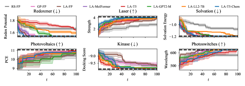
Figure 3: LLM as fixed feature extractor in BO over molecules. See Figure 2(a) for the model’s schematic.

A popular example of PEFT is LoRA (Hu et al., 2022), which uses a bottleneck architecture to introduce additional parameters in a LLM. Let ${\bm{W}}_{*}\in\mathbb{R}^{D\times N}$ be an attention weight matrix. LoRA freezes it and then augments it into

$${\bm{W}}={\bm{W}}_{*}+{\bm{B}}^{\top}{\bm{A}};\qquad{\bm{A}}\in\mathbb{R}^{Z\times N},{\bm{B}}\in\mathbb{R}^{Z\times D}.$$ (5)

The additional weights in ${\bm{A}},{\bm{B}}$ are thus few for a small $Z$. Note that, many other PEFT methods are also commonly used in practice, e.g., Adapter (Houlsby et al., 2019), Prefix Tuning (Li & Liang, 2021), IA3 (Liu et al., 2022), etc.

3 Experiment Setup

Equipped with the necessary background knowledge from Section 2, we are now ready to discuss our experiments in an attempt to answer our main question on whether LLMs are good for BO in molecular discovery. Refer to Algorithm 1 for the problem statement.

Datasets We evaluate the models considered (see below) on the following datasets that represent realistic problem sets from molecular materials discovery: minimizing (i) the redox potential (redoxmer) and (ii) solvation energy (solvation) of possible flow battery electrolytes (Agarwal et al., 2021), (iii) minimizing the docking score of kinase inhibitors for drug discovery (Graff et al., 2021), (iv) maximization of the fluorescence oscillator strength of lasers (Strieth-Kalthoff et al., 2023), (v) maximization of the power conversion efficiency (PCE) of photovoltaics materials (Lopez et al., 2016), and (vi) maximization of the $\pi$-$\pi^{*}$ transition wavelength of organic photoswitches (Griffiths et al., 2022). For each virtual library of molecules above, a physics-inspired simulation has been performed by the respective authors, which we use here as the ground truth $f({\bm{x}})$. Note that these problem sets cover a series of different physical properties of molecules and therefore represent a diverse set of molecular design tasks.

Features and LLMs We use the following standard non-LLM, chemistry-specific baselines: 1024-bit Morgan fingerprints (Morgan, 1965) as a chemistry-specific (non-learned) algorithmic vectorization scheme, and the feature vectors from the pretrained MolFormer transformer (Ross et al., 2022). Meanwhile, for the general-purpose LLMs, we use various recent architectures of varying sizes: T5-Base (T5, Raffel et al., 2020), GPT2-Medium (GPT2-M, Radford et al., 2019), and LLAMA-2-7B (LL2-7B, Touvron et al., 2023a). Finally, we use the work of Christofidellis et al. (2023, T5-Chem) to represent domain-specific LLMs.

Prompts For text-based surrogate models, we additionally consider several prompting functions $c({\bm{x}})$, mapping a molecule ${\bm{x}}$ to a sentence. They are (i) just-smiles which contains just the SMILES (Weininger, 1988) representation of ${\bm{x}}$, (ii) completion which treat the predicted $f({\bm{x}})$ as a completion to the sentence, (iii) naive which asks the LLM for $f({\bm{x}})$, and (iv) single-number which augments naive with an additional command to the LLM to only output numbers. (Details in LABEL:app:subsec:prompts.) Unless specified explicitly, the default prompt we use is just-smiles.

4 How Informative are Pretrained LLMs?

First, we study the out-of-the-box, non-finetuned capability of LLMs for BO. To this end, we treat an LLM as a fixed feature extractor: Given a pretrained LLM, remove its language-modeling head and obtain the function $\phi_{{\bm{W}}_{*}}$, mapping a textual context $c({\bm{x}})$ of a molecule ${\bm{x}}$ into its final transformer embedding vector $\phi_{{\bm{W}}_{*}}(c({\bm{x}}))\in\smash{\mathbb{R}^{H}}$. We can then apply a standard surrogate model $g_{\bm{\theta}}:\mathbb{R}^{H}\to\mathbb{R}$ like GPs or BNNs on $\smash{\mathbb{R}^{H}}$. See Figure 2(a) for the illustration and Algorithm 2 in Appendix A for the BO loop.

We use two commonly-used surrogate models over the fixed LLM and non-LLM features: (i) a GP with the Tanimoto and the Matérn kernels for the fingerprints and LLM/MolFormer features, respectively (Griffiths et al., 2023), and (ii) a Laplace approximated $3$-layer ReLU NN with $50$ hidden units on each layer, following the finding of Li et al. (2023). Thompson sampling is used throughout since it is general purpose and increasingly popular in chemistry applications (Hernández-Lobato et al., 2017).

4.1 General or domain-specific LLMs?

We present our first set of results in Figure 3. First, we notice that on fingerprint features, the LA is competitive with or better than GP on the majority of the problems. Thus we only consider the LA as the surrogate for LLM features.

We note that features obtained from general-purpose LLMs (T5, GPT2-M, and LLAMA-2-7B) tend to underperform compared to the simple fingerprints baseline. This indicates that although general-purpose LLMs seem to “understand” chemistry as illustrated in Figure 1, the features encoded by these LLMs are less informative for chemistry-focused BO. Note that, while this conclusion holds in our specific problem setup, LLMs do seem to be useful for more general problems (Gruver et al., 2023; Han et al., 2023).

Meanwhile, chemistry-specific transformers’ features (T5-Chem, MolFormer), are generally better-suited than the general-purpose ones. Indeed, T5-Chem features provide the best performance in most problems. Notably, T5-Chem also outperforms the non-LLM, chemistry-specific transformer MolFormer in most cases. The T5-Chem model is larger than MolFormer ($220$M vs. $44$M parameters). However, MolFormer is trained using more data ($100$M vs. $33$M). Thus, it seems that indeed the natural language-focused T5-Chem provides a better inductive bias for BO than the non-natural-language transformer in MolFormer.

4.2 Multiobjective optimization

In addition to the single-objective problems we studied in Sections 4 and 5, we perform multiobjective BO experiments by (i) combining both objectives in the flow battery problem above, and (ii) adding an extra maximization objective (electronic gap) to the laser problem. We refer to these problems as multi-redox and multi-laser, respectively.

To accommodate the additional objectives, we cast the problems as multi-output regression problems—for each ${\bm{x}}$, the posterior of $g({\bm{x}})$ is thus a multivariate Gaussian over $\mathbb{R}^{C}$ where $C$ is the number of the objectives. For the acquisition function, we use the scalarized Thompson sampling (Paria et al., 2020) with a fixed, uniform weighting.

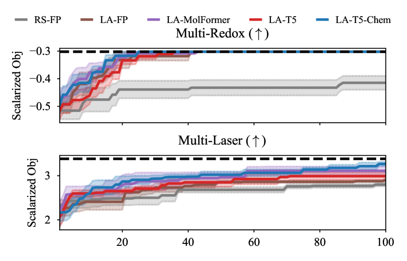
Figure 4: Scalarized multiobjective performance.

The results are provided in Figure 4. We found that the chemistry-specific transformer-based models (MolFormer, T5-Chem) are better than the general one (T5). Moreover, T5-Chem yields slightly better performance than MolFormer: better in multi-laser while performing similarly in multi-redox. Thus, our conclusion here is consistent with the one from the single-objective experiments.

4.3 Effects of prompting

We present the results of the question of how prompting affects the BO performance in Figure 5 (see also LABEL:fig:prompts_full in the appendix for the rest of the problems).

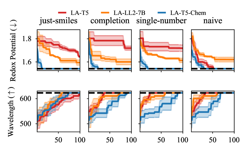
Figure 5: BO results across prompts. Top: Redoxmer, bottom: Photoswitches. Results for the other datasets are in LABEL:app:subsec:prompts.

Prompting does indeed make a difference: Unlike general LLMs (T5, LLAMA-2-7B), the chemistry-specific T5-Chem works best when the prompt is simply the SMILES string itself. Nevertheless, we note that T5-Chem obtains the best performance in most of the problems considered and across all prompts—see both Figures 5 and LABEL:fig:prompts_full. Thus the chemistry-specific T5-Chem both yield better BO performance while not requiring us to do prompt engineering.

In LABEL:fig:smiles_vs_iupac and LABEL:fig:iupac_prompts in LABEL:app:sec:results, we show results with IUPAC string representation of molecules instead of SMILES. Note that IUPAC strings are closer to natural language than SMILES, e.g. H${}_{2}$SO${}_{4}$ has IUPAC name “sulfuric acid” and SMILES representation “OS(=O)(=O)O”. We draw a similar conclusion as in the preceding section that the choice of which string representation to use is LLM-dependent. For T5-Chem, SMILES is preferable, consistent with how it was pretrained (Christofidellis et al., 2023).

4.4 The case of in-context learning

Finally, we compare the surrogate models previously studied against the recently proposed in-context learning (ICL) optimizer method of Ramos et al. (BO-LIFT, 2023). BO-LIFT works purely by prompting chat-based models such as GPT-4 (OpenAI, 2023) and LLAMA-2-7B (Touvron et al., 2023b, the chat version). Details are in LABEL:app:subsec:incontext_baselines.

We note that the uncertainty estimates yielded by BO-LIFT are obtained based on the variability in the decoding steps of the LLM. They are thus not Bayesian since they still arise from a point-estimated model. In contrast, all the Bayesian surrogates we consider in this work approximate the posterior distribution over the LLM’s weights.

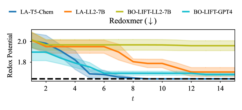
Figure 6: Fixed-feature BO surrogates vs. the in-context-learning optimizer of (Ramos et al., 2023) on the Redoxmer dataset.

We present the result of the subsampled Redoxmer dataset in Figure 6 ($|\mathcal{D_{\mathrm{cand}}}|=200,|\mathcal{D}_{1}|=5,T=15$; see Algorithm 1). We find that BO-LIFT is ineffective when combined with LLAMA-2-7B. Meanwhile, it performs much better with GPT-4, indicating that ICL requires a very large, expensive LLM. Indeed, each optimization run costs between USD $12$-$18$ for GPT-4, totalling to USD $75.81$ over $5$ random seeds. This is why we subsampled the dataset.

In contrast, using a chemistry-specific, small ($200$M parameters) T5-Chem as a feature extractor for a principled BO surrogate is better and much cheaper. Indeed, T5-Chem can be run on even mid-range consumer-grade GPUs and the LA or GP surrogate’s training can be done on CPUs.

5 How Useful are Finetuned LLMs?

In the previous section, we have seen that we can use a LLM as a fixed feature extractor in a BO loop with standard surrogate models. Here, we answer the question of whether or not treating the whole LLM itself as the surrogate model improves BO. The hypothesis is that we can improve the previous BO performance since we are performing feature learning—adapting the LLM feature to the problem at hand.

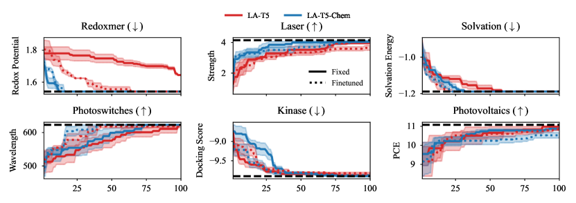
Figure 7: Finetuned LLMs as surrogate models, compared to the fixed-feature surrogates from Section 4.

However, how should we compute the posterior $p(g_{t}\mid\mathcal{D}_{t})$ in this case? Let $g_{\bm{\theta}}=\mathsf{Head}_{{\bm{w}}}\circ\varphi_{{\bm{W}}}$ be an LLM feature extractor with weights ${\bm{W}}$ along with a regression head $\mathsf{Head}_{\bm{w}}$ with weights ${\bm{w}}$—here, ${\bm{\theta}}=\{{\bm{W}},{\bm{w}}\}$. Given the dataset $\mathcal{D}_{t}$ at time $t$, the seemingly most straightforward way to perform finetuning on $g_{\bm{\theta}}$ and obtaining its posterior is to do a Bayesian updating on the previous posterior of ${\bm{W}}$ using new observations in $\mathcal{D}_{t}$ (Shwartz-Ziv et al., 2022). However, this means that we must already have a posterior over ${\bm{W}}$ in the first place—this is a very costly undertaking.

Recall that a more tractable way to introduce a feature learning on $g_{\bm{\theta}}$ is to leverage PEFT. However, unlike full finetuning, it breaks the nice Bayesian posterior updating interpretation on ${\bm{W}}$. In particular, how should one incorporate the pretrained LLM weights ${\bm{W}}_{*}$ into the Bayesian inference over the PEFT weights? Here, we generalize the work of Yang et al. (2023), which applied the LA on LoRA weights, to make it applicable to any PEFT method in general.

We do so by treating the original LLM’s weights ${\bm{W}}$ as hyperparameters and performing Bayesian inference only on ${\bm{w}}$ and the PEFT weights $\bm{\omega}$. Specifically, let $g_{\bm{\theta}}=\mathsf{Head}_{{\bm{w}}}\circ\varphi_{\bm{\omega},{\bm{W}}_{*}}$ with ${\bm{\theta}}=\{{\bm{w}},\bm{\omega}\}$ be the new surrogate model, and ${\bm{W}}_{*}$ be the pretrained LLM weights. We define:

In other words, the pretraining weights ${\bm{W}}_{*}$ act as conditioning variables on the PEFT, just like any other hyperparameters. The usual training procedure, i.e. finding the optimal PEFT weights ${\bm{\theta}}_{*}$, can then be seen as MAP estimation under this probabilistic framework. While this formulation is rather obvious after the fact, so far, it has not been clarified in previous work. Indeed, a clear interpretation of Bayesian PEFT in relation to Bayesian updating in full finetuning has been missing, even from the work of Yang et al. (2023).

Notice that any Bayesian methods can be used to approximate the posterior in (6). In this work, we use the LA: Given the weight-space LA posterior $p({\bm{\theta}}\mid\mathcal{D};{\bm{W}}={\bm{W}}_{*})$ over the PEFT weights, we can obtain the PEFT posterior predictive $p(g_{t}\mid\mathcal{D}_{t};{\bm{W}}_{*})$ via the LLA (2). This step is tractable since the Jacobian matrix $\smash{{\bm{J}}_{*}}({\bm{x}})$ is only of size $C\times\smash{\widehat{P}}$, where $C$ is the number of BO objectives (much fewer than the language-modeling head’s outputs) and $\smash{\widehat{P}}$ is the PEFT parameters (much fewer than the LLM’s parameters).

Finally, the clarity given by the formulation (6) might also give the LA a further benefit: Since ${\bm{W}}$ is now a hyperparameter, i.e. it is part of $\gamma$ in (3), one can further optimize it (or a subset of it) via the marginal likelihood if one so choose. This can potentially improve performance, similar to deep kernel learning (Wilson et al., 2016) in the context of GPs, although makes PEFT training as expensive as full finetuning. We leave this for future work since our present focus is on the usage of LLMs, and not on a new method arising from the probabilistic model in (6).

5.1 Are finetuned LLM surrogates preferable?

Following (Yang et al., 2023), we use LoRA as the PEFT method of choice: For each time $t$, we reinitialize and train the LoRA weights with MAP estimation (1) using the observed molecules $\mathcal{D}_{t}$, and then apply the LLA to obtain the posterior predictive distribution $p(g_{t}\mid\mathcal{D}_{t})$. See Figure 2(b) and Algorithm 3 for an illustration and pseudocode, respectively. See also LABEL:app:subsec:trainings for the training details. We compare the resulting finetuned surrogates with their fixed-feature surrogate counterparts from Section 4.

In Figure 7, we show the finetuning results on T5 and T5-Chem, representing general-purpose and chemistry-specific LLMs, respectively. We found that finetuning is indeed beneficial for both cases. Notice that finetuning improves the BO performance in most problems compared to the fixed-feature version.

On the flip side, notice also that in some cases, finetuning does not significantly improve the non-finetuning version. Moreover, in one problem (Photovoltaics), we found that finetuning decreases the performance of T5-Chem. We attribute this to the fact that we use the same hyperparameters (learning rate, weight decay, etc. of LoRA’s SGD and the LA) on all problems, which is closer to practice: One often simply uses the default hyperparameters of a BO algorithm provided by a software package such as BoTorch (Balandat et al., 2020). In any case, it is encouraging to see that finetuning generally works well across most BO problems considered with their default hyperparameters.

The cost of each BO iteration $t$ is largely bottlenecked by the forward passes over the candidate molecules in $\mathcal{D_{\mathrm{cand}}}$ (Algorithm 1, line 3), and not the finetuning and Laplace approximation of the surrogate, see LABEL:fig:timing in LABEL:app:sec:results. This is because $|\mathcal{D_{\mathrm{cand}}}|$ can be several orders of magnitude larger than $|\mathcal{D}_{t}|$ during the BO loop, and even forward passes on LLMs are already expensive. Moreover, due to GPU memory limitation, one can only use a small minibatch size—$16$ in our case. In contrast, fixed-feature surrogates do not have this problem since one can simply cache the LLM’s features to be used for all iterations $t$. Nevertheless, this can be alleviated via engineering efforts such as by parallelizing the forward passes over $\mathcal{D_{\mathrm{cand}}}$.

6 Related Work

While LLMs have been leveraged for BO (Ramos et al., 2023; Anonymous, 2023), so far they have only been used in a heuristic manner: The uncertainty estimates are obtained from the softmax probabilities outputted by a point-estimated (i.e., non-Bayesian) LLM. The closest work to ours is Ranković & Schwaller (2023) which studied the usage of text embeddings for BO with GP surrogates. However, the goals of their work and the present work are different: Here, we investigate whether the usage of LLMs is justified for BO due to their apparent chemistry question-answering capability, and not just to study the usage of text embeddings. Furthermore, Ranković & Schwaller (2023) did not study the effect of prompting and finetuning. Finally, the present work can be seen as an extension to the work of Yang et al. (2023): We provide a clear probabilistic interpretation and generalize their work, and use it in the context of BO instead of natural language processing tasks.

Besides the discrete BO, one can cast BO over molecules into a continuous optimization problem with the help of generative models. Gómez-Bombarelli et al. (2018); Tripp et al. (2020); Maus et al. (2022) employed variational autoencoder to construct a continuous latent representation of molecules and then performed BO on the said latent space. Moreover, the training of the surrogate model and the autoencoder can also be done jointly (Stanton et al., 2022). Unlike those methods, we focus on studying the role of language models and view the problem as a much simpler yet still practically relevant discrete BO.

7 Conclusion

We have shown that large language models (LLMs) do indeed carry useful information to aid Bayesian optimization (BO) over molecules. However, this usefulness was only apparent when one (i) uses a chemistry-specific LLM or (ii) performs finetuning—preferably both. Indeed, for point (i), even when the recent LLAMA-2-7B LLM was used as a feature extractor for a BO surrogate or when the state-of-the-art GPT-4 was used in conjunction with in-context learning, the optimization performance was subpar compared to that of a much smaller chemistry-focused LLM’s features. We addressed point (ii) by providing a way to formulate Bayesian inference for general parameter-efficient finetuning (PEFT), which in turn enables principled uncertainty estimation over LLMs with any PEFT method. We found that these principled BO surrogates are effective and yet much cheaper than in-context learning methods since small domain-specific LLMs can be used. We hope that our findings and the accompanying software library can be useful for practitioners and arouse further principled methods around LLMs for scientific discovery both inside and outside of chemistry. It is also interesting to investigate the underlying mechanism of how LLMs induce good exploration-exploitation tradeoffs.

Appendices

Appendix A Additional Details

A.1 Pseudocodes

We present the pseudocode of the BO loop corresponding to Figure 2(a) and Section 4 in Algorithm 2. Meanwhile, the pseudocode corresponding to Figure 2(b) and Section 5 is in Algorithm 3.

Algorithm 2 Using an LLM as a feature extractor in BO.

Pre-trained LLM feature extractor $\phi_{{\bm{W}}_{*}}$, mapping a context $c({\bm{x}})$to its last transformer embedding vector ${\bm{h}}\in\smash{\mathbb{R}^{H}}$; prompting function $c$mapping a molecule ${\bm{x}}$to a textual prompt; surrogate model $g_{\bm{\theta}}:\smash{\mathbb{R}^{H}}\to\mathbb{R}$; candidate molecules $\mathcal{D_{\mathrm{cand}}}=\{{\bm{x}}_{i}\}_{i=1}^{n}$; initial dataset $\mathcal{D}_{1}=\{({\bm{x}}_{i},f({\bm{x}}_{i}))\}_{i=1}^{m}$; time budget $T$. $t=1,\dots,T$$\varPhi_{t}=\{(\phi_{{\bm{W}}_{*}}(c({\bm{x}})),f({\bm{x}})):({\bm{x}},f({\bm{x}}))\in\mathcal{D}_{t}\}$$p(g_{t}\mid\mathcal{D}_{t})=\mathtt{infer}(g_{\bm{\theta}},\varPhi_{t})$E.g. via GP or the LLA ${\bm{x}}_{t}=\operatorname*{arg\,max}_{{\bm{x}}\in\mathcal{D_{\mathrm{cand}}}}\alpha(p(g_{t}(c({\bm{x}}))\mid\mathcal{D}_{t}))$$\mathcal{D}_{t+1}=\mathcal{D}_{t}\cup\{({\bm{x}}_{t},f({\bm{x}}_{t}))\}$$\mathcal{D_{\mathrm{cand}}}=\mathcal{D_{\mathrm{cand}}}\setminus\{{\bm{x}}_{t}\}$$\operatorname*{arg\,max}_{({\bm{x}},f({\bm{x}}))\in\mathcal{D}_{T+1}}f({\bm{x}})$

Algorithm 3 LLM and PEFT as a surrogate model in BO.

An LLM with a regression head $g_{\bm{\theta}}$; prompting function $c$mapping a molecule ${\bm{x}}$to a textual prompt; candidate molecules $\mathcal{D_{\mathrm{cand}}}=\{{\bm{x}}_{i}\}_{i=1}^{n}$; initial dataset $\mathcal{D}_{1}=\{({\bm{x}}_{i},f({\bm{x}}_{i}))\}_{i=1}^{m}$; time budget $T$. $t=1,\dots,T$$\mathcal{C}_{t}=\{(c({\bm{x}}),f({\bm{x}})):({\bm{x}},f({\bm{x}}))\in\mathcal{D}_{t}\}$$p({\bm{\theta}}\mid\mathcal{D}_{t};{\bm{W}}={\bm{W}}_{*})=\mathtt{LA}(g_{\bm{\theta}},\mathcal{C}_{t})$Consisting of both the training (via SGD) and the Laplace approx. of the PEFT weights $p(g_{t}\mid\mathcal{D}_{t})=\mathtt{LLA}(p({\bm{\theta}}\mid\mathcal{D}_{t};{\bm{W}}={\bm{W}}_{*}))$Eq. (2

References

- Agarwal et al. (2021) Agarwal, G., Doan, H. A., Robertson, L. A., Zhang, L., and Assary, R. S. Discovery of energy storage molecular materials using quantum chemistry-guided multiobjective bayesian optimization. Chemistry of Materials, 33(20), 2021.
- Angello et al. (2023) Angello, N., Friday, D., Hwang, C., Yi, S., Cheng, A., Torres-Flores, T., Jira, E., Wang, W., Aspuru-Guzik, A., Burke, M., and et al. Closed-loop transfer enables AI to yield chemical knowledge. ChemRxiv, 2023.
- Anonymous (2023) Anonymous. Large language models to enhance Bayesian optimization. In Submitted to ICLR, 2023. URL https://openreview.net/forum?id=OOxotBmGol. under review.
- Auer et al. (2002) Auer, P., Cesa-Bianchi, N., and Fischer, P. Finite-time analysis of the multi-armed bandit problem. Machine Learning, 47, 2002.
- Balandat et al. (2020) Balandat, M., Karrer, B., Jiang, D., Daulton, S., Letham, B., Wilson, A. G., and Bakshy, E. BoTorch: A framework for efficient Monte-Carlo Bayesian optimization. In NeurIPS, 2020.
- Bender et al. (2021) Bender, E. M., Gebru, T., McMillan-Major, A., and Shmitchell, S. On the dangers of stochastic parrots: Can language models be too big? In ACM Conference on Fairness, Accountability, and Transparency, 2021.
- Botev et al. (2017) Botev, A., Ritter, H., and Barber, D. Practical Gauss-Newton optimisation for deep learning. In ICML, 2017.
- Brown et al. (2020) Brown, T., Mann, B., Ryder, N., Subbiah, M., Kaplan, J. D., Dhariwal, P., Neelakantan, A., Shyam, P., Sastry, G., Askell, A., et al. Language models are few-shot learners. In NeurIPS, 2020.
- Chalkidis et al. (2020) Chalkidis, I., Fergadiotis, M., Malakasiotis, P., Aletras, N., and Androutsopoulos, I. LEGAL-BERT: The muppets straight out of law school. In EMNLP, 2020.
- Chithrananda et al. (2020) Chithrananda, S., Grand, G., and Ramsundar, B. ChemBERTa: Large-scale self-supervised pretraining for molecular property prediction. arXiv preprint arXiv:2010.09885, 2020.
- Christofidellis et al. (2023) Christofidellis, D., Giannone, G., Born, J., Winther, O., Laino, T., and Manica, M. Unifying molecular and textual representations via multi-task language modelling. In ICML, 2023.
- Daxberger et al. (2021) Daxberger, E., Kristiadi, A., Immer, A., Eschenhagen, R., Bauer, M., and Hennig, P. Laplace redux – effortless Bayesian deep learning. In NeurIPS, 2021.
- de Regt (2020) de Regt, H. W. Understanding, values and the aims of science. Philosophy of Science, 87(5), 2020.
- Enamine Ltd. (2023) Enamine Ltd. The Enamine REAL database, 2023. URL https://enamine.net/compound-collections/real-compounds/real-database. Accessed: 2023-11-29.
- Fortuin et al. (2022) Fortuin, V., Garriga-Alonso, A., Ober, S. W., Wenzel, F., Rätsch, G., Turner, R. E., van der Wilk, M., and Aitchison, L. Bayesian neural network priors revisited. In ICLR, 2022.
- Garnett (2023) Garnett, R. Bayesian optimization. Cambridge University Press, 2023.
- Gómez-Bombarelli et al. (2018) Gómez-Bombarelli, R., Wei, J. N., Duvenaud, D., Hernández-Lobato, J. M., Sánchez-Lengeling, B., Sheberla, D., Aguilera-Iparraguirre, J., Hirzel, T. D., Adams, R. P., and Aspuru-Guzik, A. Automatic chemical design using a data-driven continuous representation of molecules. ACS central science, 4(2), 2018.
- Gorgulla et al. (2023) Gorgulla, C., Nigam, A., Koop, M., Çınaroğlu, S. S., Secker, C., Haddadnia, M., Kumar, A., Malets, Y., Hasson, A., Li, M., Tang, M., Levin-Konigsberg, R., Radchenko, D., Kumar, A., Gehev, M., Aquilanti, P.-Y., Gabb, H., Alhossary, A., Wagner, G., Aspuru-Guzik, A., Moroz, Y. S., Fackeldey, K., and Arthanari, H. VirtualFlow 2.0 - the next generation drug discovery platform enabling adaptive screens of 69 billion molecules. bioRxiv, 2023.
- Graff et al. (2021) Graff, D. E., Shakhnovich, E. I., and Coley, C. W. Accelerating high-throughput virtual screening through molecular pool-based active learning. Chemical Science, 12(22), 2021.
- Greenaway et al. (2023) Greenaway, R. L., Jelfs, K. E., Spivey, A. C., and Yaliraki, S. N. From alchemist to AI chemist. Nature Reviews Chemistry, 7(8), 2023.
- Griffiths et al. (2022) Griffiths, R.-R., Greenfield, J. L., Thawani, A. R., Jamasb, A. R., Moss, H. B., Bourached, A., Jones, P., McCorkindale, W., Aldrick, A. A., Fuchter, M. J., and Lee, A. A. Data-driven discovery of molecular photoswitches with multioutput Gaussian processes. Chemical Science, 13(45), 2022.
- Griffiths et al. (2023) Griffiths, R.-R., Klarner, L., Moss, H. B., Ravuri, A., Truong, S., Stanton, S., Tom, G., Rankovic, B., Du, Y., Jamasb, A., Deshwal, A., Schwartz, J., Tripp, A., Kell, G., Frieder, S., Bourached, A., Chan, A., Moss, J., Guo, C., Durholt, J., Chaurasia, S., Strieth-Kalthoff, F., Lee, A. A., Cheng, B., Aspuru-Guzik, A., Schwaller, P., and Tang, J. GAUCHE: A library for Gaussian processes in chemistry. In NeurIPS, 2023.
- Gruver et al. (2023) Gruver, N., Finzi, M., Qiu, S., and Wilson, A. G. Large language models are zero-shot time series forecasters. In NeurIPS, 2023.
- Guo et al. (2023) Guo, T., Guo, K., Nan, B., Liang, Z., Guo, Z., Chawla, N. V., Wiest, O., and Zhang, X. What can large language models do in chemistry? A comprehensive benchmark on eight tasks. arXiv preprint arXiv:2305.18365, 2023.
- Han et al. (2023) Han, C., Wang, Z., Zhao, H., and Ji, H. In-context learning of large language models explained as kernel regression. arXiv preprint arXiv:2305.12766, 2023.
- Hernández-Lobato et al. (2017) Hernández-Lobato, J. M., Requeima, J., Pyzer-Knapp, E. O., and Aspuru-Guzik, A. Parallel and distributed Thompson sampling for large-scale accelerated exploration of chemical space. In ICML, 2017.
- Hickman et al. (2023) Hickman, R., Parakh, P., Cheng, A., Ai, Q., Schrier, J., Aldeghi, M., and Aspuru-Guzik, A. Olympus, enhanced: Benchmarking mixed-parameter and multi-objective optimization in chemistry and materials science. ChemRxiv, 2023.
- Hickman et al. (2022) Hickman, R. J., Aldeghi, M., Häse, F., and Aspuru-Guzik, A. Bayesian optimization with known experimental and design constraints for chemistry applications. Digital Discovery, 1(5), 2022.
- Houlsby et al. (2019) Houlsby, N., Giurgiu, A., Jastrzebski, S., Morrone, B., De Laroussilhe, Q., Gesmundo, A., Attariyan, M., and Gelly, S. Parameter-efficient transfer learning for NLP. In ICML, 2019.
- Hu et al. (2022) Hu, E. J., Shen, Y., Wallis, P., Allen-Zhu, Z., Li, Y., Wang, S., Wang, L., and Chen, W. LoRA: Low-rank adaptation of large language models. In ICLR, 2022.
- Häse et al. (2021) Häse, F., Aldeghi, M., Hickman, R. J., Roch, L. M., and Aspuru-Guzik, A. Gryffin: An algorithm for Bayesian optimization of categorical variables informed by expert knowledge. Applied Physics Reviews, 8(3), 2021.
- Immer et al. (2021) Immer, A., Korzepa, M., and Bauer, M. Improving predictions of Bayesian neural nets via local linearization. In AISTATS, 2021.
- Jablonka et al. (2023) Jablonka, K. M., Schwaller, P., Ortega-Guerrero, A., and Smit, B. Leveraging large language models for predictive chemistry. ChemRxiv, 2023.
- Jacot et al. (2018) Jacot, A., Gabriel, F., and Hongler, C. Neural tangent kernel: Convergence and generalization in neural networks. In NIPS, 2018.
- Jones et al. (1998) Jones, D. R., Schonlau, M., and Welch, W. J. Efficient global optimization of expensive black-box functions. Journal of global optimization, 13, 1998.
- Kasneci et al. (2023) Kasneci, E., Seßler, K., Küchemann, S., Bannert, M., Dementieva, D., Fischer, F., Gasser, U., Groh, G., Günnemann, S., Hüllermeier, E., et al. ChatGPT for good? on opportunities and challenges of large language models for education. Learning and Individual Differences, 103, 2023.
- Kim et al. (2022) Kim, S., Lu, P. Y., Loh, C., Smith, J., Snoek, J., and Soljačić, M. Deep learning for Bayesian optimization of scientific problems with high-dimensional structure. TMLR, 2022.
- Kingma & Ba (2015) Kingma, D. P. and Ba, J. Adam: A method for stochastic optimization. In ICLR, 2015.
- Korovina et al. (2020) Korovina, K., Xu, S., Kandasamy, K., Neiswanger, W., Poczos, B., Schneider, J., and Xing, E. P. ChemBO: Bayesian optimization of small organic molecules with synthesizable recommendations. In AISTATS, 2020.
- Kristiadi et al. (2023) Kristiadi, A., Immer, A., Eschenhagen, R., and Fortuin, V. Promises and pitfalls of the linearized Laplace in Bayesian optimization. In Advances in Approximate Bayesian Inference, 2023.
- Li & Liang (2021) Li, X. L. and Liang, P. Prefix-tuning: Optimizing continuous prompts for generation. In ACL, 2021.
- Li et al. (2023) Li, Y. L., Rudner, T. G., and Wilson, A. G. A study of Bayesian neural network surrogates for Bayesian optimization. arXiv preprint arXiv:2305.20028, 2023.
- Liu et al. (2022) Liu, H., Tam, D., Muqeeth, M., Mohta, J., Huang, T., Bansal, M., and Raffel, C. A. Few-shot parameter-efficient fine-tuning is better and cheaper than in-context learning. In NeurIPS, 2022.
- Lopez et al. (2016) Lopez, S. A., Pyzer-Knapp, E. O., Simm, G. N., Lutzow, T., Li, K., Seress, L. R., Hachmann, J., and Aspuru-Guzik, A. The harvard organic photovoltaic dataset. Scientific Data, 3(160086), 2016.
- Loshchilov & Hutter (2017) Loshchilov, I. and Hutter, F. SGDR: Stochastic gradient descent with warm restarts. In ICLR, 2017.
- Lyu et al. (2019) Lyu, J., Wang, S., Balius, T. E., Singh, I., Levit, A., Moroz, Y. S., O’Meara, M. J., Che, T., Algaa, E., Tolmachova, K., Tolmachev, A. A., Shoichet, B. K., Roth, B. L., and Irwin, J. J. Ultra-large library docking for discovering new chemotypes. Nature, 566(7743), 2019.
- MacKay (1992a) MacKay, D. J. The evidence framework applied to classification networks. Neural Computation, 4(5), 1992a.
- MacKay (1992b) MacKay, D. J. A practical Bayesian framework for backpropagation networks. Neural Computation, 4(3), 1992b.
- Maik Jablonka et al. (2023) Maik Jablonka, K., Ai, Q., Al-Feghali, A., Badhwar, S., Bran, J. D., Bringuier, S., Brinson, L. C., Choudhary, K., Circi, D., Cox, S., et al. 14 examples of how LLMs can transform materials science and chemistry: A reflection on a large language model hackathon. arXiv preprint arXiv:2306.06283, 2023.
- Mangrulkar et al. (2022) Mangrulkar, S., Gugger, S., Debut, L., Belkada, Y., Paul, S., and Bossan, B. PEFT: State-of-the-art parameter-efficient fine-tuning methods. https://github.com/huggingface/peft, 2022.
- Maus et al. (2022) Maus, N., Jones, H., Moore, J., Kusner, M. J., Bradshaw, J., and Gardner, J. Local latent space Bayesian optimization over structured inputs. In NeurIPS, 2022.
- Močkus (1975) Močkus, J. On Bayesian methods for seeking the extremum. In Optimization Techniques IFIP Technical Conference, 1975.
- Morgan (1965) Morgan, H. L. The generation of a unique machine description for chemical structures-a technique developed at chemical abstracts service. Journal of Chemical Documentation, 5(2), 1965.
- OpenAI (2023) OpenAI. GPT-4 technical report. arXiv preprint arXiv:2303.08774, 2023.
- Paria et al. (2020) Paria, B., Kandasamy, K., and Póczos, B. A flexible framework for multi-objective Bayesian optimization using random scalarizations. In UAI, 2020.
- Pyzer-Knapp et al. (2015) Pyzer-Knapp, E. O., Suh, C., Gómez-Bombarelli, R., Aguilera-Iparraguirre, J., and Aspuru-Guzik, A. What is high-throughput virtual screening? A perspective from organic materials discovery. Annual Review of Materials Research, 45(1), 2015.
- Radford et al. (2019) Radford, A., Wu, J., Child, R., Luan, D., Amodei, D., Sutskever, I., et al. Language models are unsupervised multitask learners. OpenAI Blog, 2019.
- Raffel et al. (2020) Raffel, C., Shazeer, N., Roberts, A., Lee, K., Narang, S., Matena, M., Zhou, Y., Li, W., and Liu, P. J. Exploring the limits of transfer learning with a unified text-to-text transformer. JMLR, 21(1), 2020.
- Ramos et al. (2023) Ramos, M. C., Michtavy, S. S., Porosoff, M. D., and White, A. D. Bayesian optimization of catalysts with in-context learning. arXiv preprint arXiv:2304.05341, 2023.
- Ranković & Schwaller (2023) Ranković, B. and Schwaller, P. BoChemian: Large language model embeddings for Bayesian optimization of chemical reactions. In NeurIPS 2023 Workshop on Adaptive Experimental Design and Active Learning in the Real World, 2023.
- Rasmussen & Williams (2005) Rasmussen, C. E. and Williams, C. K. I. Gaussian processes in machine learning. 2005.
- Restrepo (2022) Restrepo, G. Chemical space: limits, evolution and modelling of an object bigger than our universal library. Digital Discovery, 1(5), 2022.
- Ritter et al. (2018) Ritter, H., Botev, A., and Barber, D. A scalable Laplace approximation for neural networks. In ICLR, 2018.
- Ross et al. (2022) Ross, J., Belgodere, B., Chenthamarakshan, V., Padhi, I., Mroueh, Y., and Das, P. Large-scale chemical language representations capture molecular structure and properties. Nature Machine Intelligence, 4(12), 2022.
- Schneider (2010) Schneider, G. Virtual screening: An endless staircase? Nature Reviews Drug Discovery, 9(4), 2010.
- Sharir et al. (2020) Sharir, O., Peleg, B., and Shoham, Y. The cost of training NLP models: A concise overview. arXiv preprint arXiv:2004.08900, 2020.
- Shoichet (2004) Shoichet, B. K. Virtual screening of chemical libraries. Nature, 432(7019), 2004.
- Shwartz-Ziv et al. (2022) Shwartz-Ziv, R., Goldblum, M., Souri, H., Kapoor, S., Zhu, C., LeCun, Y., and Wilson, A. G. Pre-train your loss: Easy Bayesian transfer learning with informative priors. In NeurIPS, 2022.
- Snoek et al. (2012) Snoek, J., Larochelle, H., and Adams, R. P. Practical Bayesian optimization of machine learning algorithms. In NIPS, 2012.
- Stanton et al. (2022) Stanton, S., Maddox, W., Gruver, N., Maffettone, P., Delaney, E., Greenside, P., and Wilson, A. G. Accelerating Bayesian optimization for biological sequence design with denoising autoencoders. In ICML, 2022.
- Strieth-Kalthoff et al. (2023) Strieth-Kalthoff, F., Hao, H., Rathore, V., Derasp, J., Gaudin, T., Angello, N. H., Seifrid, M., Trushina, E., Guy, M., Liu, J., and et al. Delocalized, asynchronous, closed-loop discovery of organic laser emitters. ChemRxiv, 2023.
- Sun et al. (2019) Sun, C., Huang, L., and Qiu, X. Utilizing BERT for aspect-based sentiment analysis via constructing auxiliary sentence. In NAACL, 2019.
- Thompson (1933) Thompson, W. R. On the likelihood that one unknown probability exceeds another in view of the evidence of two samples. Biometrika, 25(3-4), 1933.
- Tom et al. (2024) Tom, G., Schmid, S. P., Baird, S. G., Cao, Y., Darvish, K., Hao, H., Lo, S., Pablo-Garcia, S., Rajaonson, E. M., Skreta, M., Yoshikawa, N., Corapi, S., Akkoc, G. D., Strieth-Kalthoff, F., Seifrid, M., and Aspuru-Guzik, A. Self-driving laboratories for chemistry and materials sciences. ChemRxiv, 2024.
- Touvron et al. (2023a) Touvron, H., Lavril, T., Izacard, G., Martinet, X., Lachaux, M.-A., Lacroix, T., Rozière, B., Goyal, N., Hambro, E., Azhar, F., et al. LLaMA: Open and efficient foundation language models. arXiv preprint arXiv:2302.13971, 2023a.
- Touvron et al. (2023b) Touvron, H., Martin, L., Stone, K., Albert, P., Almahairi, A., Babaei, Y., Bashlykov, N., Batra, S., Bhargava, P., Bhosale, S., et al. Llama 2: Open foundation and fine-tuned chat models. arXiv preprint arXiv:2307.09288, 2023b.
- Tripp et al. (2020) Tripp, A., Daxberger, E., and Hernández-Lobato, J. M. Sample-efficient optimization in the latent space of deep generative models via weighted retraining. In NeurIPS, 2020.
- Vaswani et al. (2017) Vaswani, A., Shazeer, N., Parmar, N., Uszkoreit, J., Jones, L., Gomez, A. N., Kaiser, L., and Polosukhin, I. Attention is all you need. In NIPS, 2017.
- Vig et al. (2021) Vig, J., Madani, A., Varshney, L. R., Xiong, C., Socher, R., and Rajani, N. F. BERTology meets biology: Interpreting attention in protein language models. In ICLR, 2021.
- Wang et al. (2023) Wang, H., Fu, T., Du, Y., Gao, W., Huang, K., Liu, Z., Chandak, P., Liu, S., Katwyk, P. V., Deac, A., Anandkumar, A., Bergen, K., Gomes, C. P., Ho, S., Kohli, P., Lasenby, J., Leskovec, J., Liu, T.-Y., Manrai, A., Marks, D., Ramsundar, B., Song, L., Sun, J., Tang, J., Velickovic, P., Welling, M., Zhang, L., Coley, C. W., Bengio, Y., and Zitnik, M. Scientific discovery in the age of artificial intelligence. Nature, 620(7972), 2023.
- Weininger (1988) Weininger, D. Smiles, a chemical language and information system. 1. introduction to methodology and encoding rules. Journal of Chemical Information and Computer Sciences, 28(1), 1988.
- Wilson et al. (2016) Wilson, A. G., Hu, Z., Salakhutdinov, R., and Xing, E. P. Deep kernel learning. In AISTATS, 2016.
- Wolf et al. (2019) Wolf, T., Debut, L., Sanh, V., Chaumond, J., Delangue, C., Moi, A., Cistac, P., Rault, T., Louf, R., Funtowicz, M., et al. Huggingface’s transformers: State-of-the-art natural language processing. arXiv preprint arXiv:1910.03771, 2019.
- Yang et al. (2023) Yang, A. X., Robeyns, M., Wang, X., and Aitchison, L. Bayesian low-rank adaptation for large language models. arXiv preprint arXiv:2308.13111, 2023.
- Zhang & Lee (2019) Zhang, Y. and Lee, A. A. Bayesian semi-supervised learning for uncertainty-calibrated prediction of molecular properties and active learning. Chemical Science, 10(35), 2019.