Navigating Complexity: Toward Lossless Graph Condensation via Expanding Window Matching

Abstract

Graph condensation aims to reduce the size of a large-scale graph dataset by synthesizing a compact counterpart without sacrificing the performance of Graph Neural Networks (GNNs) trained on it, which has shed light on reducing the computational cost for training GNNs. Nevertheless, existing methods often fall short of accurately replicating the original graph for certain datasets, thereby failing to achieve the objective of lossless condensation. To understand this phenomenon, we investigate the potential reasons and reveal that the previous state-of-the-art trajectory matching method provides biased and restricted supervision signals from the original graph when optimizing the condensed one. This significantly limits both the scale and efficacy of the condensed graph. In this paper, we make the first attempt toward lossless graph condensation by bridging the previously neglected supervision signals. Specifically, we employ a curriculum learning strategy to train expert trajectories with more diverse supervision signals from the original graph, and then effectively transfer the information into the condensed graph with expanding window matching. Moreover, we design a loss function to further extract knowledge from the expert trajectories. Theoretical analysis justifies the design of our method and extensive experiments verify its superiority across different datasets. Code is released at https://github.com/NUS-HPC-AI-Lab/GEOM.

1 Introduction

Graph condensation follows the success in vision dataset distillation (Wang et al., 2018; Zhao et al., 2020; Nguyen et al., 2021; Cazenavette et al., 2022; Zhou et al., 2022, 2023) and aims to synthesize a smaller condensed graph dataset from the original one. Recently, gradient and trajectory matching methods (Jin et al., 2022a, b; Zheng et al., 2023; Hashemi et al., 2024) have achieved remarkable results on some small-scale graph datasets. For instance, SFGC (Zheng et al., 2023) condenses Citeseer (Kipf & Welling, 2016) to 1.8% sparsity without performance drop. However, these methods fail to perform well on large-scale graph datasets, i.e, there persists an unignorable performance gap between GNNs trained on the condensed and original graph datasets. This severely limits their effectiveness in real-world scenarios. Therefore, developing a high-performing and robust graph condensation approach has become urgent for broader graph-related applications.

In addressing the condensation challenges on large-scale graphs, a critical question arises: what causes the notable discrepancy in performance between condensing large-scale and small-scale graphs? To this end, we analyze the differing outcomes of previous methods applied to graphs of various sizes. A key observation highlights that a smaller condensation ratio is utilized for large-scale graphs compared to small-scale ones. This suggests a greater disparity in size between large-scale graphs and their condensed counterparts. One intuitive solution is to enlarge the condensation ratio. We conduct experiments with the existing methods and show results in Fig. 1. However, we find that the performance of the condensed graph saturates as the ratio increases. Besides, a significant gap still exists between the saturated performance and that of the original graph.

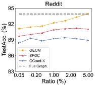
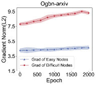
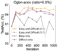
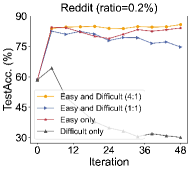
Figure 1: (a) shows that the performances in previous methods (Jin et al., 2022b; Zheng et al., 2023) stop increasing after the condensation ratio in large-scale graph dataset reaches a certain threshold. (b) shows that the gradient generated by easy nodes and difficult nodes during the training process of the experts. (c) and (d) indicate that using supervision signals provided by solely easy nodes can yield better performance for the condensed graph than solely using difficult nodes. Nevertheless, incorporating a small portion of difficult nodes into easy ones can further enhance the performance of the condensed graph.

GCond (Jin et al., 2022b) explains this phenomenon as follows: optimizing a larger condensed graph might be more complex. Nevertheless, GCond does not specify the exact cause of this phenomenon. We infer that the lack of rich supervision from the original graph might be a potential reason. To verify it, we take trajectory matching method SFGC (Zheng et al., 2023) as an example for the following exploration. SFGC trains a set of expert trajectories on the original graph as supervision for optimizing the condensed graph. To analyze the principal components of the supervision, we visualize the gradient norm of easy and difficult nodes (categorized by homophily level (Wei et al., 2023)) from the original graph in Fig. 1. One can find that the difficult nodes dominate the principal components of supervision from the original graph. This may cause the condensed graph to exhibit a bias toward difficult nodes while overlooking easy nodes (Wang et al., 2022).

To investigate the effectiveness of different components of the supervision signals, we select four ratios of mixed easy and difficult nodes to train the expert trajectories. We report the performance comparisons of the condensed graph in Fig. 1 and 1. Several observations can be concluded as follows: 1) Only using the supervision signals from difficult nodes can not perform well; 2) Using a proper ratio of easy and difficult nodes obtains the best performance in our experiments. These observations highlight the importance of understanding the impact of node characteristics on learning dynamics in the condensed graph. In graph learning, easy nodes have representative features of the original graph, whereas difficult nodes contain ambiguous features (Wei et al., 2023). Combined with the observations, we conclude that condensed graph captures representative patterns under the supervision of easy nodes. Although proper supervision of difficult nodes further enrich the patterns, excessive supervision of them may result in chaotic features (Liu et al., 2023b, c) and damage the representative patterns.

Based on our findings, we propose a novel approach called Graph Condensation via Expanding WindOw Matching (GEOM). Specifically, we train the expert trajectories with curriculum learning to involve more diverse supervision signals from the original graph. Then, we utilize an expanding window to determine the matching range when matching trajectories. In this way, we enable the rich information of the original graph can be compactly and efficiently transferred to the condensed counterpart. Theoretical analysis justifies our design from the perspective of reducing accumulated error (Du et al., 2023). Furthermore, inspired by network distillation (Hinton et al., 2015; Zhang et al., 2021b), we design a loss function to uncover information in expert trajectories from a new perspective.

In this work, we make the first attempt toward lossless graph condensation. Concretely, we condense Citeseer to 0.9%, Cora to 1.3%, Ogbn-arxiv to 5%, Flickr to 1%, and Reddit to 5% without any performance loss when training a GCN. Moreover, our condensed graphs can generalize well to different GNN models, and even achieve lossless performance across 20 out of 35 cross-architecture experiments. We hope our work can help mitigate the heavy computation cost for training GNNs on large-scale graph datasets and broaden the real-world applications of graph condensation.

2 Method

In this section, we first briefly overview the framework of trajectory matching graph condensation and curriculum learning. Then we introduce the components of our method as well as theoretical understanding.

2.1 Preliminaries

Trajectory matching graph condensation (Zheng et al., 2023). Given a large graph dataset $\mathcal{T}$, trajectory matching graph condensation synthesizes a small graph dataset $\mathcal{S}$ by minimizing the training trajectory distance on $\mathcal{T}$ and $\mathcal{S}$. It aims to reduce the performance gap between GNNs trained on $\mathcal{T}$ and $\mathcal{S}$. Generally, trajectory matching graph condensation can be divided into three phases.

1. Buffer Phase. Preparing the expert trajectories: training GNNs on $\mathcal{T}$ and saving the checkpoints.

2. Condensation Phase. Condensing the original graph dataset: optimizing the condensed graph by matching the training trajectories between $\mathcal{T}$ and $\mathcal{S}$.

3. Evaluation Phase. Evaluating the condensed graph dataset: using the condensed graph datasets to train a randomly initialized GNN.

Formally, in the condensation phase, we optimize the following objective to synthesize the condensed graph $\mathcal{S}$:

$$\min_{S}\mathrm{E}_{\theta_{t}^{*}\sim P_{\theta_{\tau}}}\left[\mathcal{L}_{M}\left((\theta_{t}^{*}|^{t+p}_{t},\widetilde{\theta}_{t}|^{t+q}_{t})\right)\right],$$ (1)

where $\theta_{t}^{*}|^{t+p}_{t},\widetilde{\theta}_{t}|^{t+q}_{t}$ denote the parameters of GNNs trained on $\mathcal{T}$ and $\mathcal{S}$ within checkpoints $\left(t,t+p\right)$, $P_{\theta_{\tau}}$ denotes the parameter distribution with the expert trajectories. $\mathcal{L}_{M}$ is the distance between trajectories trained on $\mathcal{T}$ and $\mathcal{S}$, which can be written as:

$$\mathcal{L}_{M}=\frac{\left\|\widetilde{\theta}_{t+q}-\theta_{t+p}^{*}\right\|_{2}^{2}}{\left\|\widetilde{\theta}_{t}-\theta_{t+p}^{*}\right\|_{2}^{2}},$$ (2)

where $\widetilde{\theta}_{t}=\theta_{t}^{*}$, $\theta_{t+p}^{*}$ denotes the model parameters $p$ checkpoints after $\theta_{t}^{*}$. Meanwhile, $\widetilde{\theta}_{t+q}$ results from $q$ inner-loops using the classification loss $\ell$, applied to dataset $\mathcal{S}$, and a learnable learning rate $\eta$:

$$\widetilde{\theta}_{t+i+1}=\widetilde{\theta}_{t+i}-\eta\nabla\ell\left(f\left(\widetilde{\theta}_{t+i};\mathcal{S}\right),\mathcal{Y}\right),$$ (3)

where $f\left(;\right)$ is the GNN trained on $\mathcal{S}$, $\mathcal{Y}$ is the label set of the condensed graph dataset. Note that in the buffer phase, GNN is trained on the whole graph dataset $\mathcal{T}$ by default.

Curriculum learning. Different from the normal training scheme (Zheng et al., 2023; Cazenavette et al., 2022), the most distinctive characteristic of curriculum learning (CL) lies in differentiating the training samples (Bengio et al., 2009; Krueger & Dayan, 2009). Specifically, CL imitates how humans learn by organizing data samples in a logical sequence, primarily from easy to difficult, as the curriculum for model training (Wei et al., 2023; Wang et al., 2021b). Prior works demonstrate that CL steers models to a more optimal parameter space (Li et al., 2023; Bengio et al., 2009) than normal training. CL can enhance model performance, generalization, robustness, and even convergence in diverse scenarios (Sitawarin et al., 2021; Weinshall & Amir, 2020; Krishnapriyan et al., 2021).

2.2 Preparing Curriculum-based Expert Trajectories

The superiority of CL has been demonstrated across various tasks, prompting us to integrate CL into graph condensation. Taking a closer look at CL, it allows the model to initially focus on easy samples and then gradually shift attention to more difficult ones, thereby forming expert trajectories with more diverse supervision signals. To implement the CL approach, we design a difficulty measurer based on homophily to differentiate between easy and difficult samples. Moreover, we utilize a continuous training scheduler to sequence the samples into an easy-to-difficult curriculum.

Homophily-based difficulty measurer. On node classification tasks, GNNs learn node representation through an iterative process of aggregating neighborhood information (Ma et al., 2021; Halcrow et al., 2020). Owing to this mechanism, the nodes tend to aggregate features from neighbors sharing the same class will receive additional information about their class features. Thus, GNNs are more adept at learning these nodes as they will have more representative features (Chien et al., 2020; Zhu et al., 2020). Conversely, for nodes aggregate features from neighbors in many different classes, their representations become chaotic, making them hard to learn (Maurya et al., 2021; Mao et al., 2023).

Thus, inspired by CLNode (Wei et al., 2023), we calculate the difficulty score for each node through the label distribution of its neighborhood to distinguish between easy and difficult. Specifically, for each training node $x$, the difficulty score can be calculated as follows:

$$\mathcal{P}_{c}(x)=\frac{|\{y_{n}=c|n\in\mathcal{N}(x)\cup\{x\}\wedge y_{n}\in\mathcal{Y}\}|}{|{\mathcal{N}}(x)\cup\{x\}|},$$ (4)

$$\mathcal{D}(x)=-\sum_{c\in C}P_{c}(x)log(P_{c}(x)),$$ (5)

Where $y_{n}$ denotes the label of node $n$, $\mathcal{P}_{c}(x)$ represents the proportion of neighborhood nodes $\mathcal{N}(x)\cup x$ in class $c$. The difficulty score $\mathcal{D}(x)$ is higher as the neighbor nodes of node $x$ become more diverse (as illustrated in Fig 2).

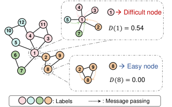
Figure 2: An example of homophily-based difficulty measurer.

Curriculum training scheduler. After getting the difficulty score, we utilize a continuous training scheduler to generate an easy-to-difficult curriculum for training expert trajectories. Specifically, we use a pacing function to map each epoch $t$ to a scalar $\lambda_{t}$ in (0, 1], and then select a proportion $\lambda_{t}$ of the easiest nodes for training at epoch $t$. More details of the pacing function is detailed in Appendix B. Furthermore, we do not stop training when the whole graph training set is involved, as the recently added nodes may not have been sufficiently learned at this time. Specifically, we persist in training with the whole graph training set until the validation set accuracy converges.

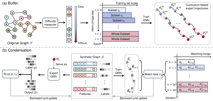
Figure 3: Overall framework of GEOM. In the buffer phase, we train the expert trajectories with curriculum learning to involve more informative supervision signals from the original graph. In the condensation phase, we utilize expanding window matching to capture the rich information. Moreover, a knowledge embedding extractor is used to further extract knowledge from the expert trajectories.

2.3 Expanding Window Matching

Since we obtain expert trajectories with more diverse supervision signals through CL in the buffer phase, we aim to fully utilize the rich information embedded in them to optimize the condensed graph. One straightforward way is to gradually move the matching range (we can sample the expert trajectory segments that need to be matched from this range) later to shift the focus of the condensed graph from primarily learning from easy nodes to difficult nodes.

However, such a matching strategy significantly degrades the performance of the condensed graph (as shown in Table 3). One potential reason is: once the whole matching range is shifted later, the condensed graph falls into the trap of learning patterns from the difficult nodes continually, thereby collapsing the representative patterns.

To address the challenge of effectively learning patterns from easy and difficult nodes, we propose to use an adaptive window that gradually expands the matching range instead of a fixed sliding window, termed expanding window matching. Formally, we determine the matching range $\mathcal{R}$ as:

$$\mathcal{R}=\begin{cases}\{\theta_{0}^{*}\ldots\theta_{U+p}^{*}\},&\quad{I}<{U}\\ \{\theta_{0}^{*}\ldots\theta_{U+p}^{*}\;\theta_{U+p+I}^{*}\},&\quad{I}\geq{U}\wedge{I}<{U^{{}^{\prime}}},\\ \{\theta_{0}^{*}\ldots\theta_{U+p}^{*}\ldots\theta_{U^{\prime}+p}^{*}\},&\quad{I}\geq{U^{{}^{\prime}}}\end{cases}$$ (6)

where $I$ denotes the number of the iteration in the condensation phase, ${U}$ and ${U^{{}^{\prime}}}$ are two different upperbounds to control the size of the matching range.

Expanding window matching ensures that in the early stages of condensation, the main component of supervision signals is from easy nodes, allowing the condensed graph to initially learn representative patterns. In the later stages of condensation, the condensed graph can maintain these representative patterns while enriching them. This is because the matching strategy efficiently controls the weight of easy and difficult nodes in supervision signals, the condensed graph has the opportunity to learn from both of them.

From another perspective, in the previous method, the matching range is confined to a very narrow scope, causing only a few checkpoints can be utilized. In contrast, the proposed expanding window matching brings 10 times more available checkpoints than before, thereby more effectively utilizing the information provided by expert trajectories.

Next, we provide the theoretical analysis to demonstrate the advantages of employing CL in the buffer phase and the expanding window matching in the condensation phase.

Theoretical understanding. In the condensation phase, the trajectory on $\mathcal{S}$ is optimized to reproduce the trajectory on $\mathcal{T}$ with $\widetilde{\theta}_{t}=\theta_{t}^{*}$. However, in the evaluation phase, the starting points are no longer initialized by the parameters on $\mathcal{T}$ and the parameters are continually updated by $\mathcal{S}$. The error accumulates progressively in the evaluation phase, which leads to greater divergence between the final parameters of GNNs trained on $\mathcal{S}$ and $\mathcal{T}$. Thus, reducing this error helps improve the final performance of $\mathcal{S}$.

Following Du et al. (2023), we first divide the training trajectories into $N$ stages to be matched, denoted as $\{\theta^{*}_{0,0},...,\theta^{*}_{0,p},\theta^{*}_{1,0},...,\theta^{*}_{N-1,p}\}$, where the last parameter of a previous stage is the starting parameter of the next stage, i.e. $\theta^{*}_{n,0}=\theta^{*}_{n-1,p}$. The training trajectory of GNNs trained on $\mathcal{S}$ can also be divided into corresponding $N$ stages similarly. For any given stage $n$, the following definition apply:

Definition 2.1.

Accumulated error $\epsilon_{n}$ refers to the difference in model parameters trained on condensed and original graphs at stage $n$ during the evaluation phase:

$$\epsilon_{n}=\widetilde{\theta}_{n,q}-\theta^{*}_{n,p}=\widetilde{\theta}_{n+1,0}-\theta^{*}_{n+1,0},$$ (7)

To specifically analyze the accumulated error, we introduce two additional error terms as follows:

Definition 2.2.

Initialization error $I$ refers to the discrepancies caused by varying initial parameters during the training process. Specifically, even if the condensed graph can generate identical trajectories to the original, variations at the trajectories’ endpoints are unavoidable due to the differing starting points in the condensation phase compared to the evaluation phase, i.e. $\widetilde{\theta}_{n,0}=\theta^{*}_{n,0}+\epsilon_{n-1}$. To simplify the notation, we denote the parameter changes of the GNN trained for $p$ rounds on $T$ and $q$ rounds on $S$ as $\Theta_{S}(\theta_{0},q)=\sum^{q}_{i=0}\bigtriangledown_{\theta}L_{S}(f_{\theta_{0+i}})$ and $\Theta_{T}(\theta_{0},p)=\sum^{p}_{i=0}\bigtriangledown_{\theta}L_{T}(f_{\theta_{0+i}})$, respectively. Then, the initialization error at stage $n$ is:

$$I_{n}=I(\theta^{*}_{n,0},\epsilon_{n-1})=\Theta_{S}(\theta^{*}_{n,0}+\epsilon_{n-1},q)-\Theta_{S}(\theta^{*}_{n,0},q),$$ (8)

Definition 2.3.

Matching error $\delta$ refers to differences at the endpoints of the same stage in the training trajectories of GNNs trained on $\mathcal{T}$ and $\mathcal{S}$ during the condensation phase:

$$\delta_{n+1}=\Theta_{S}(\theta^{*}_{n,0},q)-\Theta_{T}(\theta^{*}_{n,0},p).$$ (9)

The following theorem elucidates the relation among errors:

Theorem 2.4.

During the evaluation phase, the accumulated error at any stage is determined by its initial value and the sum of matching error and initialization error starting from the second stage.

$$\epsilon_{n+1}=\sum^{n}_{i=1}I({\theta^{*}_{i,0},\epsilon_{i-1}})+\sum^{n}_{i=0}\delta_{i+1}+\epsilon_{0}.$$ (10)

The proof for the above theorem can be found in Appendix C.1. In the previous condensation method, only a few stages of the expert trajectory are selected to optimize the condensed graph. Assuming the sum of matching errors is optimized to $\mu$ in the condensation phase, the optimized accumulated error can be formulated as:

$$\epsilon^{*}_{n+1}=\sum^{n}_{i=1}I({\theta^{*}_{i,0},\epsilon_{i-1}})+\mu+\epsilon_{0}.$$ (11)

Corollary 2.5.

The proposed strategy can optimize the accumulated error in both the buffer and condensation phases.

Proof.

According to (Du et al., 2023), flatter training trajectories reduce initialization error and can be derived from the following equation:

$$\begin{split}\theta^{*}_{n,i}&=\arg\min_{\theta^{*}_{n,i}}||I(\theta^{*}_{n,i},\epsilon_{n-1})||^{2}\\ &\approx\arg\min_{\theta^{*}_{n,i}}\{\mathcal{L}_{M}(f\left(\theta^{*}_{n,i}\right)+\alpha S(\theta^{*}_{n,i})\}\end{split}$$ (12)

where $\alpha$ as the coefficient that balances the robustness of $\theta^{*}$ to the perturbation, and $S(\theta)$ as the sharpness of the loss landscape. CL has been demonstrated in smoothing the loss landscape (Sinha et al., 2020; Zhang et al., 2021a). Since we employ CL in the buffer phase, we reduce $S(\theta)$ efficiently, thereby reducing accumulated error.

Moreover, employing expanding window matching to determine the matching range can involve more stages in the expert trajectories as matching targets. This enables the direct optimization of $\delta_{n}$, thereby reducing the sum of matching errors $\mu^{{}^{\prime}}$. When conducting expanding window matching, multiple simulations of the evaluation phase can be involved in the condensation phase, i.e., training GNNs on $\mathcal{S}$ and $\mathcal{T}$ starting from $\theta^{*}_{0,0}$, then minimize the matching error of this stage. This allows for the effective optimization of $\epsilon_{0}$ and $I({\theta^{*}_{1,0},\epsilon_{0}})$ in the condensation stage as well.

$$\epsilon^{*^{\prime}}_{n+1}=\sum^{n}_{i=1}I^{{}^{\prime}}({\theta^{*}_{i,0},\epsilon_{i-1}})+\mu^{\prime}+\epsilon^{{}^{\prime}}_{0}<\epsilon^{*}_{n+1}.$$ (13)

Where $\epsilon^{{}^{\prime}}$, $I^{\prime}$, $\mu^{{}^{\prime}}$ are the reduced $\epsilon$, $I$, $\mu$ respectively. The above corollary suggests that using CL in the buffer phase and expanding window matching in the condensation phase can effectively reduce the accumulated error during the evaluation phase. ∎

Algorithm 1 GEOM for condensing graph.

1:Input: Original graph dataset $\mathcal{T}$.

2:Require: $\{\tau_{p}\}$: A set of expert trajectories obtained by training ${\mathrm{GNN}}_{\mathcal{T}}$ on the original graph dataset $\mathcal{T}$ with a curriculum learning schema. $p$: numbers of the training steps of the GNNs trained on $\mathcal{S}$ in each inner-loop optimization. $q$: numbers of the checkpoints between the start and target parameters. ${U},{U^{{}^{\prime}}}$: two upper bounds to determine the matching range.

3:Initialize condensed graph $\mathcal{S}$.

4:for $k=0,\ldots,K-1$ do

5:     Randomly sample a expert trajectory $\tau_{p}\sim\{\tau_{p}\}$

6:     Randomly sample $\theta_{t}^{*}$ and $\theta_{t+p}^{*}$, where $0<t\leq{U}$

7:     Initialize $\widetilde{\theta}_{t},\widetilde{\theta}_{t}=\theta_{t}^{*}$

8:     for $i=0,\ldots,q-1$ do

9:         training GNNs on $\mathcal{S}$ and update $\widetilde{\theta}_{t+i}$

10:         through Eq. 3

11:     end for

12:     Update condensed graph $\mathcal{S}$ through Eq. 15

13:     if   ${U}<{U^{{}^{\prime}}}$ then

14:          ${U}={U}+1$

15:end for

16:Output: Condensed graph dataset $\mathcal{S}$.

Table 1: Performance comparison to baselines in the node classification tasks. We achievethe highest results in most cases on node classification and lossless results on all datasets. We report test accuracy (%) on Citeseer, Cora, Ogbn-arxiv, Flickr and Reddit. Bold entries are best results, highlight marks the lossless results. Some experiments appear out of memory (oom).

Dataset	Ratio ($r$)	Random	Herding	K-Center	DC-Graph	GCond	GCond-X	SFGC	GEOM	Whole Dataset
Citeseer	0.90%	54.4±4.4	57.1±1.5	52.4±2.8	66.8±1.5	70.5±1.2	71.4±0.8	71.4±0.5	73.0±0.5	71.7±0.1
	1.80%	64.2±1.7	66.7±1.0	64.3±1.0	59.0±0.5	70.6±0.9	69.8±1.1	72.4±0.4	74.3±0.1
	3.60%	69.1±0.1	69.0±0.1	69.1±0.1	66.3±1.5	69.8±1.4	69.4±1.4	70.6±0.7	73.3±0.4
Cora	1.30%	63.6±3.7	67.0±1.3	64.0±2.3	67.3±1.9	79.8±1.3	75.9±1.2	80.1±0.4	82.5±0.4	81.2±0.2
	2.60%	72.8±1.1	73.4±1.0	73.2±1.2	67.6±3.5	80.1±0.6	75.7±0.9	81.7±0.5	83.6±0.3
	5.20%	76.8±0.1	76.8±0.1	76.7±0.1	67.7±2.2	79.3±0.3	76.0±0.3	81.6±0.8	82.8±0.7
Ogbn-arxiv	0.05%	47.1±3.9	52.4±1.8	47.2±3.0	58.6±0.4	59.2±1.1	61.3±0.5	65.5±0.7	65.5±0.6	71.4±0.1
	0.25%	57.3±1.1	58.6±1.2	56.8±0.8	59.9±0.3	63.2±0.3	64.2±0.4	66.1±0.4	68.8±0.2
	0.50%	60.0±0.9	60.4±0.8	60.3±0.4	59.5±0.3	64.0±1.4	63.1±0.5	66.8±0.4	69.6±0.2
	2.50%	64.1±0.7	64.3±0.8	64.1±0.5	61.3±0.3	66.3±1.1	66.1±0.3	68.3±0.3	71.0±0.1
	5.00%	66.0±0.6	66.1±0.4	66.2±0.3	66.7±0.3	oom	66.9±0.4	69.4±0.3	71.4±0.1
Flickr	0.10%	41.8±2.0	42.5±1.8	42.0±0.7	46.3±0.2	46.5±0.4	45.9±0.1	46.6±0.2	47.1±0.1	47.2±0.1
	0.50%	44.0±0.4	43.9±0.9	43.2±0.1	45.9±0.1	47.1±0.1	45.0±0.2	47.0±0.1	47.0±0.2
	1.00%	44.6±0.2	44.4±0.6	44.1±0.4	44.6±0.1	47.1±0.1	45.0±0.2	47.1±0.1	47.3±0.3
Reddit	0.01%	46.1±4.4	53.1±2.5	46.6±2.3	88.2±0.2	88.0±1.8	88.4±0.4	89.7±0.2	91.1±0.4
	0.10%	58.0±2.2	62.7±1.0	53.0±3.3	89.5±0.1	89.6±0.7	89.3±0.1	90.0±0.3	91.4±0.2	93.9±0.0
	0.20%	66.3±1.9	71.0±1.6	58.5±2.1	90.5±1.2	90.1±0.5	88.8±0.4	90.3±0.3	91.5±0.4
	3.00%	78.4±1.3	81.3±1.1	82.2±1.4	90.8±0.9	oom	89.2±0.2	91.0±0.3	93.7±0.1
	5.00%	83.6±1.1	88.1±0.8	88.3±1.2	91.5±0.7	oom	88.9±0.3	91.9±0.2	93.9±0.1

2.4 Knowledge Embedding Extractor

To further utilize the supervision signals in the expert trajectories, inspired by network distillation (Hinton et al., 2015; Zhang et al., 2021b), we propose Knowledge Embedding Extraction (KEE), aiming to transfer the knowledge about the original dataset from well-trained GNNs into the condensed graph. Specifically, we first assign soft labels to the condensed graph, which are generated by well-trained GNNs with parameters chosen from the tails of expert trajectories. During the optimization of $\mathcal{S}$, we calculate the following loss term:

$$\mathcal{L}_{E}=\mathcal{D}_{KL}\left(f\left(\theta_{T}^{*};\mathcal{S}\right)\parallel\widetilde{\mathcal{Y}}\right),$$ (14)

Where ${\mathcal{D}}_{KL}(\cdot||\cdot)$ represents the Kullback-Leibler (KL) divergence, $\widetilde{\mathcal{Y}}$ denotes the soft labels. By incorporating such a matching loss, we further uncovered information embedded in the expert trajectories from a unique perspective.

2.5 Final Objective and Algorithm

To sum up, the total optimization objective of GEOM is:

$$\min_{S}\mathrm{E}_{\theta_{t}^{*}\sim P_{\theta_{\tau}}}\left[\mathcal{L}\left((\theta_{t}^{*}|^{t+p}_{t},\widetilde{\theta}_{t}|^{t+q}_{t}),(\mathcal{S},\widetilde{\mathcal{Y}})\right)\right],\mathrm{where}$$ (15)

$$\begin{split}\mathcal{L}&=\mathcal{L}_{M}+\alpha\mathcal{L}_{E}\\ &=\frac{\left\|\widetilde{\theta}_{t+q}-\theta_{t+p}^{*}\right\|_{2}^{2}}{\left\|\widetilde{\theta}_{t}-\theta_{t+p}^{*}\right\|_{2}^{2}},+\alpha\mathcal{D}_{KL}\left(f\left(\theta_{T}^{*};\mathcal{S}\right)\parallel\widetilde{\mathcal{Y}}\right).\end{split}\vspace{-10.0pt}$$ (16)

The pipeline of the proposed GEOM is detailed in Alg. 1.

3 Experiments

Table 2: Performance across different GNN architectures. and : the average performance and the standard deviation of the results of all architectures, denotes the improvements upon the DC-Graph. GCN indicates that the synthetic graph is condensed with GCN. Bold entries are best results.

		Architectures							Statistics
Datasets	Methods	MLP	GAT	APPNP	Cheby	GCN	SAGE	SGC	Avg.	Std.	$\Delta$(%)
	DC-Graph	66.2	-	66.4	64.9	66.2	65.9	69.6	66.5	1.5	-
	GCond	63.9	55.4	69.6	68.3	70.5	66.2	70.3	66.3	5.0	$\downarrow$ 0.2
	SFGC	71.3	72.1	70.5	71.8	71.6	71.7	71.8	71.5	0.5	$\uparrow$ 5.0
Citeseer	GEOM	74.2	74.2	74.0	74.1	74.3	74.1	74.3	74.2	0.1	$\uparrow$ 7.7
($r$ = 1.80%)	DC-Graph	67.2	-	67.1	67.7	67.9	66.2	72.8	68.1	2.1	-
	GCond	73.1	66.2	78.5	76.0	80.1	78.2	79.3	75.9	4.5	$\uparrow$ 7.8
	SFGC	81.1	80.8	78.8	79.0	81.1	81.9	79.1	80.3	1.2	$\uparrow$ 12.2
Cora	GEOM	83.6	82.7	82.8	80.7	83.6	83.7	83.1	82.9	1.0	$\uparrow$ 14.8
($r$ = 2.60%)	DC-Graph	59.9	-	60.0	55.7	59.8	60.0	60.4	59.3	1.6	-
	GCond	62.2	60.0	63.4	54.9	63.2	62.6	63.7	61.4	2.9	$\uparrow$ 2.1
	SFGC	65.1	65.7	63.9	60.7	65.1	64.8	64.8	64.3	1.6	$\uparrow$ 5.0
Ogbn-arxiv	GEOM	68.8	66.4	65.8	62.5	68.8	68.9	66.4	66.8	2.1	$\uparrow$ 7.5
($r$ = 0.25%)	DC-Graph	61.2	-	61.4	58.3	61.1	60.9	61.3	60.7	1.1	-
	SFGC	69.4	69.6	68.7	64.7	69.4	69.4	69.1	68.5	1.6	$\uparrow$7.8
Ogbn-arxiv	GEOM	71.2	70.0	69.1	64.5	71.4	71.1	69.6	69.6	2.2	$\uparrow$ 8.9
($r$ = 5.00%)	DC-Graph	43.1	-	45.7	43.8	45.9	45.8	45.6	45.0	1.1	-
	GCond	44.8	40.1	45.9	42.8	47.1	46.2	46.1	44.7	2.3	$\downarrow$ 0.3
	SFGC	47.1	45.3	40.7	45.4	47.1	47.0	42.5	45.0	2.3	-
Flickr	GEOM	47.0	42.1	46.6	45.3	47.3	47.1	46.3	46.0	1.7	$\uparrow$ 1.0
($r$ = 0.50%)	DC-Graph	50.3	-	81.2	77.5	89.5	89.7	90.5	79.8	14.0	-
	GCond	42.5	60.2	87.8	75.5	89.4	89.1	89.6	76.3	17.1	$\downarrow$ 3.5
	SFGC	89.5	87.1	88.3	82.8	89.7	90.3	89.5	88.2	2.4	$\uparrow$ 8.4
Reddit	GEOM	91.4	90.0	87.9	82.7	91.4	91.4	89.3	89.2	2.9	$\uparrow$ 9.4
($r$ = 0.10%)	DC-Graph	52.3	-	84.1	81.2	90.3	90.6	90.9	81.6	13.6	-
	SFGC	91.6	90.3	91.1	85.3	91.9	91.6	90.9	90.4	2.1	$\uparrow$8.8
Reddit	GEOM	93.9	93.0	92.4	88.5	93.9	93.8	92.7	92.6	1.8	$\uparrow$ 11.0
($r$ = 5.00%)

3.1 Setup

Datasets & architectures. We conduct experiments on three transductive datasets, i.e., Cora, Citeseer (Kipf & Welling, 2016) and Ogbn-arxiv (Hu et al., 2020), and two inductive datasets, i.e, Flickr (Zeng et al., 2020) and Reddit (Hamilton et al., 2017). For all five datasets, we use the public splits and setups. More details of each dataset can be found in Appendix A. We select APPNP (Gasteiger et al., 2018), GCN (Kipf & Welling, 2016), SGC (Wu et al., 2019), GraphSAGE (Hamilton et al., 2017). Cheby (Defferrard et al., 2016) and GAT (Veličković et al., 2017), as well as a standard MLP for cross-architecture experiments.

Baselines. We compare our method to seven baselines: 1) Coreset selection methods: Random; Herding (Welling, 2009); K-Center (Farahani & Hekmatfar, 2009; Sener & Savarese, 2017). 2) State-of-the-art condensation methods: the graph-based variant DC-Graph of vision dataset condensation (Zhao et al., 2020); gradient matching graph condensation method GCond (Jin et al., 2022b); GCond-X, the variant of GCond, which do not optimize the structure of the condensed graph; trajectory matching graph condensation method SFGC (Zheng et al., 2023).

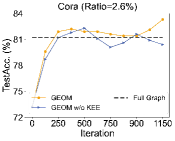
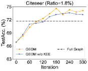
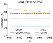
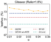
Figure 4: (a) and (b) illustrate the ablation study on whether to use the KEE. (c) and (d) illustrate the ablation of the tunable hyperparameter $\alpha$, which determines the weights of the optimization item generated by the KEE.

Implementation & evaluation. We initially employ the eight methods to synthesize condensed graphs, subsequently assessing the performance of GNNs across different datasets and architectures. In the condensation phase, GNNs are both commonly-used GCN model (Kipf & Welling, 2016). In the evaluation phase, we train a GNN on the condensed graph and then evaluate the GNN on the test set of the corresponding original graph dataset to get the performance. We report the average performance and variance on Table 1 with repeated 10 times experiments, where the GNN models used are all 2-layer GCN models with 256 hidden units. More hyper-parameter setting details are provided in Appendix E.

3.2 Results

Node classification. We compare our method with the baselines across all condensation ratios on node classification, as reported in Table 1. Our method achieves state-of-the-art results in 18 out of 19 experimental cases and brings non-trivial improvements up to 2.8%. Notably, in all datasets, we achieve lossless graph condensation below or at a 5% condensation ratio for the first time. The results confirm that the proposed GEOM can provide more informative supervision signals from the original graph for optimizing the condensed graph in the condensation phase, allowing us to get an optimal substitute for the original graph dataset.

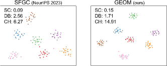
(a) Cora, $r$=5.2%

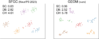
(b) Citeseer, $r$=3.6%

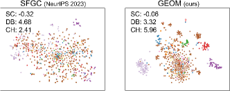
(c) Reddit, $r$=0.2%

Figure 5: T-SNE visualization on the condensed graph. Nodes of the same class are in the same color. SC$\uparrow$, DB$\downarrow$, and CH$\uparrow$ in the figure refer to the Silhouette Coefficient, Davies-Bouldin Index, and Calinski-Harabasz Index respectively. $\uparrow$ and $\downarrow$ denote the clustering pattern is better when the value is higher or lower.

Cross-architecture generalization. We evaluate the test performance of our condensed graphs across different GNN architectures. The results are reported in Table 2, showing that our condensed graphs do not overfit in the GNN architecture used in the buffer and condensation phase, they can generalize well on all other GNN architectures in our experiments. It is noteworthy that our condensed graph can even achieve lossless performance in 20 out of 35 cases, which opens up possibilities for the widespread real-world application of graph condensation. As our approach shows that it is possible to condense graphs without tailoring the condensation to specific GNN architectures separately. The performance of the whole dataset across different architectures can be found in Appendix A.

3.3 Ablation

Evaluating expanding window matching.

We compare expanding window matching to two fixed matching (Fixed1 with its starting point fixed at 0, Fixed2 at a later stage) and a sliding window matching. Additionally, we conduct the ablation on whether to use CL in the buffer phase. The results in Table 3 show that: 1) Utilizing expanding window matching solely in the condensation phase can yield better results compared to other matching strategies; 2) Fixed matching can not collaborate well with the expert trajectories trained with CL; 3) The combination of using CL and expanding window matching can bring non-trivial improvements.

Table 3: Ablation on expanding window matching.

Matching Range	Cora		Citeseer
	w/o CL	CL	w/o CL	CL
Fixed1	82.3±0.4	82.6±0.2	72.1±0.2	72.4±0.1
Fixed2	81.8±0.5	81.9±0.3	71.3±0.1	71.3±0.3
Sliding	80.8±0.3	81.1±0.4	70.7±0.1	71.0±0.2
Expanding	82.9±0.2	83.6±0.3	73.2±0.3	74.3±0.1

Evaluating knowledge embedding extractor. We first study the condensation phase with and without KEE under the optimal $\alpha$. As illustrated in Fig. 4 and 4, due to the stable guidance KEE offers, it can further enhance the performance of the condensed graph when the previous optimization hits a bottleneck. Moreover, as shown in Fig. 4 and  4, simply determining the order of the hyper-parameter $\alpha$ can make KEE aid in condensation.

3.4 Visualization

We present the visualization results for all five datasets in Fig. 5, we can observe that our condensed graphs on Cora and Citeseer show clear clustering patterns without inter-class mixing, while that of SFGC still lack clarity in the separation between classes. This gap becomes more apparent in larger datasets, where the condensed graph of SFGC fails to show any significant clustering patterns. Conversely, our condensed graph still manages to represent clear patterns between classes and clusters within the same class.

To measure the clustering patterns more precisely, we employee three different metrics designed to assess the distinctness of the clustering pattern comprehensively: Silhouette Coefficient (Rousseeuw, 1987), Davies-Bouldin Index (Davies & Bouldin, 1979) and Calinski-Harabasz Index (Caliński & Harabasz, 1974). Our condensed graph is significantly more competitive across these three evaluation metrics. This demonstrates that our matching strategy effectively captures the patterns of both easy and difficult nodes in the original graph. More visualization results on other ratios and datasets can be found in Appendix F.

4 Related Work

Dataset Distillation & Graph Condensation. Dataset distillation (DD) is a technique to reduce the size and complexity of large-scale datasets for training deep neural networks (Qin et al., 2023). Methods in DD are majorly based on matching, such as matching gradients (Zhao et al., 2020; Liu et al., 2022b, 2023a; Zhang et al., 2023), distribution (Zhao & Bilen, 2023; Wang et al., 2023), feature (Wang et al., 2022) and training trajectories (Cazenavette et al., 2022; Du et al., 2023; Guo et al., 2023), which has led to a wide application in lots of downstream tasks (Masarczyk & Tautkute, 2020; Rosasco et al., 2021; Wang et al., 2021a). Following DD, Graph Condensation compresses the graph dataset by matching gradients (Jin et al., 2022a, b; Yang et al., 2023; Zhang et al., 2024), distribution (Liu et al., 2022a) and training trajectories (Zheng et al., 2023). For a thorough review, we refer the reader to a recent survey (Hashemi et al., 2024). However, there persists a significant performance gap to get lossless graph condensation.

5 Conclusion

In this work, we propose GEOM, a novel method for graph condensation via expanding window matching. GEOM outperforms the state-of-the-art methods across various datasets and architectures, making the first attempt toward lossless graph condensation.

Limitations and future works. GEOM still relies on deriving trajectories in advance, which incurs additional computational costs for expert GNNs training. We will explore improving the efficiency of condensing graphs in the future.

Impact Statements

Ethical impacts. There are no ethical issues in our paper, including its motivation, designs, experiments, and used data. The goal of the proposed GEOM is to advance the field of graph condensation.

Expected societal implications. Training GNNs on real-world graph data comes with a high computational cost. Graph condensation achieves more efficient computation by reducing the size of the graph data. This helps in reducing energy consumption in computing devices, thereby reducing carbon emissions, which is highly beneficial for sustainability and environmental conservation.

Appendix A Dataset Details

A.1 Statistics of Dataset

The performance assessment of our method encompasses an array of datasets, comprising three transductive datasets: Cora, Citeseer (Kipf & Welling, 2016), Ogbn-arxiv (Hu et al., 2020) and two inductive datasets: Flickr (Zeng et al., 2020) and Reddit (Hamilton et al., 2017)). These datasets are sourced from PyTorch Geometric (Fey & Lenssen, 2019), with publicly accessible splits consistently applied across all experimental setups. We first set three condensation ratios for each dataset, consistent with the setting before (Zheng et al., 2023; Jin et al., 2022b), and for Ogbn-arxiv and Reddit, we add comparisons with two additional larger condensation ratios. Dataset statistics are shown in Table 4

Table 4: Dataset statistics. The first three are transductive datasets and the last two are inductive datasets.

Dataset	#Nodes	#Edges	#Classes	#Features	Training/Validation/Test
Cora	2,708	5,429	7	1,433	140/500/1000
Citeseer	3,327	4,732	6	3,703	120/500/1000
Ogbn-arxiv	169,343	1,166,243	40	128	90,941/29,799/48,603
Flickr	89,250	899,756	7	500	44,625/22312/22313
Reddit	232,965	57,307,946	210	602	15,3932/23,699/55,334

A.2 Performance of Dataset

We show the performances of various GNNs on the original graph datasets in Table 5. Notably, our approach achieves lossless performance for 20 combinations across 35 combinations of five datasets and seven architectures

Table 5: Performances of various GNNs on original graphs. The underline signifies that the performance of our synthetic graph is the same as or better than the original graph dataset.

	MLP	GAT	APPNP	Cheby	GCN	SAGE	SGC
Citeseer	69.1	70.8	71.8	70.2	71.7	70.1	71.3
Cora	76.9	83.1	83.1	81.4	81.2	81.2	81.4
Ogbn-arxiv	67.8	71.5	71.2	71.4	71.4	71.5	71.4
Flickr	47.6	44.3	47.3	47.0	47.1	46.1	46.2
Reddit	92.6	91.0	94.3	93.1	93.9	93.0	93.5

Appendix B Datails of the Training Scheduler

After assessing node difficulty, we implement a curriculum-based approach to train a GNN model. Following CLNode (Wei et al., 2023), We introduce a continuous training scheduler that gradually increases the difficulty level in the curriculum. Specifically, we organize the training set by the ascending node difficulty. Then, using a pacing function $h(t)$ to map each epoch to a certain value $\lambda_{t}$, where $0<\lambda_{t}\leq 1$, indicating the proportion of the training nodes selected for the training subset at epoch $\zeta$. $\lambda$ represents initial proportion of the available nodes, $\zeta$ is the epoch when $h(t)$ attains the value of 1. The pacing functions are as follows:

• linear:

  $$h(t)=\min(1,\lambda+(1-\lambda)\frac{t}{\zeta}).$$ (17)

• root:

  $$h(t)=\min(1,\sqrt{\lambda^{2}+(1-\lambda^{2})\frac{t}{\zeta}}).$$ (18)

• geometrics:

  $$h(t)=\min(1,2^{log_{2}\lambda-log_{2}\lambda\frac{t}{\zeta}}).$$ (19)

Furthermore, we do not halt the training as soon as $t$ equals $\zeta$, since at this point, the knowledge of difficult nodes might not be fully embedded into the expert trajectories. Therefore, we continue to train the model for an additional period to ensure that the information of these difficult nodes is also embedded into the expert trajectories.

Appendix C Detailed Theoretical Analysis

C.1 Proof of Theorem 2.4

Theorem C.1.

During the evaluation phase, the accumulated error at any stage is determined by its initial value and the sum of matching error and initialization error starting from the second stage.

$$\epsilon_{n+1}=\sum^{n}_{i=1}I({\theta^{*}_{i,0},\epsilon_{i-1}})+\sum^{n}_{i=0}\delta_{i+1}+\epsilon_{0}.$$ (20)

Proof.

For the stage directly matched in the condensation process, we assume that its matching error can be reduced to a negligible value. Assuming the sum of matching errors for the remaining segments is $\mu$.

$$\begin{split}\epsilon_{n+1}&=\hat{\theta}_{n,q}-\theta^{*}_{n,p}\\ &=(\hat{\theta}_{n,0}+\Theta_{S}(\hat{\theta}_{n,0},q))-(\theta^{*}_{n,0}+\Theta_{T}(\theta^{*}_{n,0},p))\\ &=(\hat{\theta}_{n,0}+\Theta_{S}(\theta^{*}_{n,0}+\epsilon_{n},q))-(\theta^{*}_{n,0}+\Theta_{T}(\theta^{*}_{n,0},p))\\ &=(\hat{\theta}_{n,0}-\theta^{*}_{n,0})+(\Theta_{S}(\theta^{*}_{n,0}+\epsilon_{n},q)-\Theta_{S}(\theta^{*}_{n,0},q))+(\Theta_{S}(\theta^{*}_{n,0},q)-\Theta_{T}(\theta^{*}_{n,0},p))\\ &=\epsilon_{n}+I({\theta^{*}_{n,0},\epsilon_{t}})+\delta_{n+1}\\ &=\sum^{n}_{i=1}I({\theta^{*}_{i,0},\epsilon_{i-1}})+\sum^{n}_{i=0}\delta_{i+1}+\epsilon_{0},\end{split}$$ (21)

As shown in Equation 21, the accumulated error during the evaluation process can be represented as the result of the summation of the initial accumulated error and the sum of the matching errors and the accumulated errors, except for those that have been reduced. ∎

C.2 Detailed Analysis

In the meta-matching method proposed by SFGC, a segment of the expert trajectory is selected for trajectory matching. This approach can only utilize a small part of the information in the whole training trajectory. In our method, there are two improvements in the condensation matching phase. Firstly, we use an expanding window starting from 0 for matching, which means during the condensation phase, more stages will be matched, resulting in a smaller matching error $\mu^{{}^{\prime}}$, and the student network is trained multiple times starting from $\theta^{*}_{0,0}$, thus incorporating $\epsilon_{0}$ into the optimization. Note that when $t=0$, the definitions of accumulated error and matching error are the same, and due to the optimization of $\epsilon_{0}$, $I(\theta^{*}_{1,0},\epsilon_{0})$ is also optimized simultaneously (Du et al., 2023). More importantly, previous research has shown that curriculum learning can generate flatter training trajectories (Sinha et al., 2020; Sitawarin et al., 2021; Krishnapriyan et al., 2021; Zhang et al., 2021a), which can optimize $I(\theta^{*}_{n,0},\epsilon_{n-1})$ efficiently (Du et al., 2023).

We denote the optimized accumulated error and initialization error as $\epsilon^{{}^{\prime}}_{n}$ and $I^{\prime}$ respectively. Assuming $||I(\theta^{*}_{1,0},\epsilon_{0})-I^{\prime}(\theta^{*}_{1,0},\epsilon_{0})||=\tau_{1}>0$, $||\epsilon_{0}-\epsilon^{{}^{\prime}}_{0}||\geq\tau_{2}>0$, $||I(\theta^{*}_{i,0},\epsilon_{i-1})-I^{\prime}(\theta^{*}_{i,0},\epsilon_{i-1})||=\tau_{3}>0$ and $||\mu-\mu^{{}^{\prime}}||=\tau_{4}>0$, we have

$$\epsilon^{*^{\prime}}_{n}=\epsilon_{n}-\tau_{1}-\tau_{2}-(t^{*}-2)\tau_{3}-\tau_{4}<\epsilon^{*}_{n}.$$ (22)

This implies that our method has a smaller accumulated error during the evaluation phase, resulting in better performances.

Appendix D More Analysis

D.1 Training Samples Analysis

In our quest to identify nodes that play a dominant role in the formation of expert trajectories, we train each node in the training set sequentially through a GNN and record the gradient values generated by each node. At the same time, based on a ranking of difficulty, we classify the lowest 70% of nodes in terms of difficulty scores as easy nodes and the highest 30% as difficult nodes and compute the average gradients for easy and difficult nodes. As illustrated in Fig. 1, due to the challenge GNNs face in learning clear representations from these difficult nodes, larger gradients are produced, and the GNN tends to focus more on these nodes during training. Consequently, in expert trajectories, the supervision signals from difficult nodes are more emphasized.

To explore the distinct guiding roles of these nodes during the condensation phase, we train the GNN with different ratios of easy to difficult nodes (since we need to control the ratio while maintaining a consistent number of nodes used, we must select subsets from the whole training set) to form expert trajectories. As shown in Fig. 1 and 1, the supervision role of easy nodes is essential for optimizing the condensed graph; relying solely on difficult nodes is insufficient for optimization, as they rarely contain the general patterns of the original graph.

D.2 Time Complexity Analysis

Time complexity. We first measure the time complexity of the GCond, SFGC, and GEOM. For simplicity, let the number of GCN layers in the adjacency matrix generator be $L$, the number of the sampled neighbors per node be $r$ and all the hidden units be $d$. The number of nodes in the original graph dataset is $N$ and the number of nodes in the condensed graph dataset is $N^{{}^{\prime}}$. In the forward process, training GCN on the original graph has a complexity of $O(r^{L}Nd^{2})$ and $O(LN^{\prime 2}d+LN^{\prime}d)$ on the condensed graph. For GCond, it has time complexity of $TKO(LN^{\prime 2}d+LN^{\prime}d)+TKO(N^{\prime 2}d^{2})$, where $\zeta$ denotes the number of outermost loops, $K$ denotes the number of different initialization. For SFGC and our method, the time complexity of matching training trajectories is about $TO(LN^{\prime}d^{2}+LN^{\prime}d)$, and offline training expert GCNs have a time complexity of $MO(r^{L}Nd^{2})$, where $M$ is the number of the experts. Although our method requires calculating the loss generated by a one-time forward on the expert GCN on the condensed graph, the small size of the condensed graph means that the time for a single forward on a 2-layer GCN is almost negligible. Additionally, the expert parameters do not require extra training to obtain, so we consider the time complexity of this operation as a constant $E$.

Running time. Although our method introduces an additional constant $E$ in terms of time complexity, we have made improvements in how the condensed graph is evaluated, saving time, especially in the evaluation of larger-scale condensed graphs, thereby further enhancing the efficiency of our method. Concretely, the assessment of condensed graph-free data involves training a GNN model with it. The improved test performance of the GNN model in node classification at a particular meta-matching step suggests superior quality of the condensed data at that stage.

Consequently, this evaluation process requires training a GNN model from the ground up while evaluating the GNN’s performance at each epoch of training, which in turn incurs increased time and computational cost. To lower the computational cost, SFGC choose to use a Graph Neural Feature Score to evaluate the condensed graph. However, the Graph Neural Feature Score can only work in an extremely low condensation ratio, the greater the condensation ratio, the less pronounced the advantages of the Graph Neural Feature Score become.

Aiming to enhance the efficiency of evaluating the condensed graph, we analyze the root causes of efficiency issues with the original evaluation method. Firstly, since the size of the condensed graph is much smaller compared to the original graph dataset, as we mentioned in our time complexity analysis, the time taken for the condensed graph to forward on a GCN is very short. The majority of the time spent in the original method of training a GNN from scratch was due to testing on the original dataset’s test set in each training epoch, to determine the best-performing training epoch for the final performance.

Therefore, we design a short-term interval training evaluation to assess the performance of the condensed graph. Specifically, we do not require the GNN trained with the condensed graph to reach a well-trained state, but instead, we try to reduce the number of training epochs (e.g., training only for 200 epochs on Ogbn-arxiv) and compare the performance of condensed graphs within the same training epochs. Also, during training on condensed graphs, we do not evaluate the GNN at every epoch but do so after a considerable number of training intervals, e.g., an interval of 20 epochs. By adopting this approach, we significantly reduce computational time and enhance the efficiency of evaluating the condensed graph. All experiments are conducted five times on one single Nvidia-A100-SXM4-80GB GPU. We provide the running time of our method and SFGC in Fig. 6.

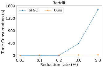
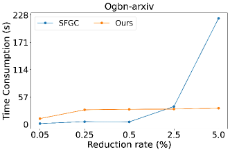
Figure 6: Comparison of methods for evaluating and storing condensed graphs.

D.3 Analysis of Matching Range

In exploring the effects of different ranges of long-term matching, we present the impacts of various step combinations of $q$ steps (student) and $p$ steps (expert) on the Ogbn-arxiv dataset, with r = 0.5%. The results, displayed in Fig. 7, show that the optimal step combination exists for 2100 student steps ($q$) and 1900 expert steps ($p$). Under this setup, the condensed graph exhibits the best node classification performance. Additionally, the quality and expressiveness of the condensed data moderately vary with different step combinations, but the variance is not overly drastic.

Moreover, regarding the different step combinations of $p$ and $q$, we observe that without using soft labels, GEOM exhibits properties similar to SFGC, where the optimal value of $q$ is usually smaller. In the choice of $p$, due to the adoption of a curriculum learning approach and expanding window matching, a smaller $p$ can often be set during the condensation.

In cases where soft labels are used, we find that increasing $q$ under the same $p$ settings generally yields better results. One potential reason is that the information in soft labels is more complex compared to hard labels and requires more optimization steps (Guo et al., 2023). Concurrently, we eliminate unnecessary storage of student model parameters, thereby avoiding excessive memory demands caused by increasing $q$.

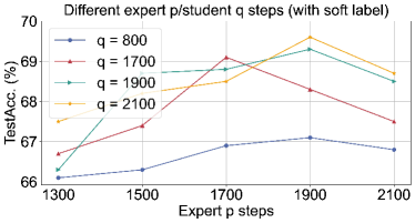
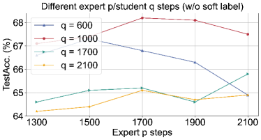
Figure 7: Performance with different step combinations of $q$ student steps and expert $p$ steps on Ogbn-arxiv ($r$ = 0.5%).

Appendix E Implementation Details

For the condensation ratio ($r$) choices, we adhere to the settings from previous studies for smaller datasets such as Cora, Citeseer, and Flickr, where our method effortlessly achieves lossless compression. Specifically, we choose 1.30%, 2.60%, 5.20% for Cora, 0.90%, 1.80%, 3.60% for Citeseer, and 0.10%, 0.50%, 0.10% for Flickr. However, for the Ogbn-arxiv and Reddit datasets, we found that the previously set condensation ratios were insufficient to involve enough information to get lossless (Jin et al., 2022b). Therefore, after conducting numerous experiments, we introduce two additional sets of condensation experiment settings for these two datasets. Specifically, we choose 0.10%, 0.50%, 1.00%, 2.50%, 5.00% for Ogbn-arxiv and 0.05%, 0.10%, 0.20%, 3.00%, 5.00% for Reddit.

In the process of training an expert trajectory, we primarily adjust three parameters to control the process of incorporating simple and difficult information: the number of epochs for training on the entire dataset ($\zeta$), the initial proportion of easy nodes ($\lambda$), and the method of gradually adding difficult nodes to the training data (Scheduler). It is worth noting that our curriculum learning approach can not improve the final performance obviously; rather, it focuses on obtaining trajectories that include clearer and more diverse information from the original graph.

During the condensation phase, we build upon SFGC by introducing parameters to control the expanding window and KEE, without specific mention, we adopt a 2-layer GCN with 256 hidden units as the GNN used for condensation. All other parameters remain consistent with those publicly disclosed for SFGC. The specific parameter settings are outlined in Table LABEL:tab:paras, where ${U^{{}^{\prime}}}$ represent the upper bounds of the expanding window, and ${U}$ denotes the upper limit of the initial expanding window, incremented by one after each condensation iteration. Notably, lr_y set to 0 indicates the absence of soft labels. An important experimental observation is that omitting early trajectory information across all datasets leads to suboptimal results. Consequently, we set the start of the expanding window to 0 consistently.

In practical implementation, we observe that soft labels can sometimes lead to optimization process instability, especially for certain small-scale condensed datasets. In such experimental scenarios, we use hard labels for the KEE process. Therefore, we do not introduce additional loss computations on this dataset.

It is important to highlight that for condensed graphs derived from Reddit and Ogbn-arxiv with condensation ratios greater than 1%, achieving optimal results requires fewer optimization iterations. A possible explanation is that when the scale of the condensed graph is larger, the gap between it and the original data can be bridged with relatively minor adjustments.

In the selection of methods for evaluating and storing condensed datasets, we don’t use the graph kernel-based method (GNTK) proposed by SFGC. This is because as the scale of condensed graphs increases, the computational time for the GNTK metric grows exponentially. When the scale of the condensed dataset is large, the time consumed to compute this metric is about six times that of training a GNN directly with the condensed graph, as illustrated in Fig. 6. Noting that to achieve a fairer comparison, we use different random seeds for the evaluation function when choosing the condensed datasets to save during the condensation phase and when assessing the performance of the condensed graphs after condensation.

Appendix F Visualizations

We showcase t-SNE plots depicting the condensed graph-free data generated by GEOM across all datasets. Our condensed graph-free data reveals a well-clustered pattern across Cora and Citeseer. Furthermore, larger-scale datasets exhibit some implicit clusters within the same class. This indicates that our approach effectively learns representative representations from the easy nodes of the original data while efficiently utilizing the difficult nodes. With the assistance of difficult nodes, the patterns become enriched.

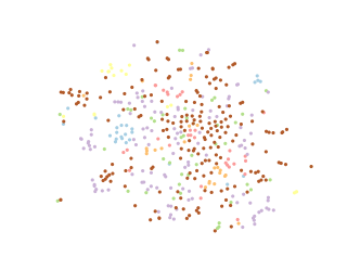
(a) Flickr, $r=1\%$

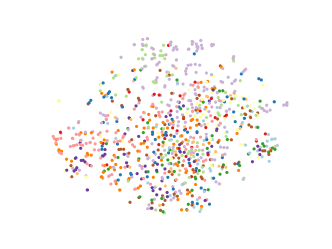
(b) Ogbn-arxiv, $r=0.5\%$

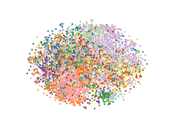
(c) Ogbn-arxiv, $r=5\%$

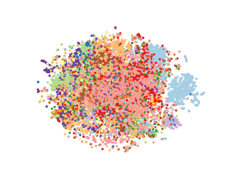
(d) Reddit, $r=5\%$

Figure 8: Visualization of t-SNE on condensed graphs

References

- Bengio et al. (2009) Bengio, Y., Louradour, J., Collobert, R., and Weston, J. Curriculum learning. In Proceedings of the 26th annual international conference on machine learning, pp. 41–48, 2009.
- Caliński & Harabasz (1974) Caliński, T. and Harabasz, J. A dendrite method for cluster analysis. Communications in Statistics-theory and Methods, 3(1):1–27, 1974.
- Cazenavette et al. (2022) Cazenavette, G., Wang, T., Torralba, A., Efros, A. A., and Zhu, J.-Y. Dataset distillation by matching training trajectories. In Proceedings of the IEEE/CVF Conference on Computer Vision and Pattern Recognition, pp. 4750–4759, 2022.
- Chien et al. (2020) Chien, E., Peng, J., Li, P., and Milenkovic, O. Adaptive universal generalized pagerank graph neural network. arXiv preprint arXiv:2006.07988, 2020.
- Davies & Bouldin (1979) Davies, D. L. and Bouldin, D. W. A cluster separation measure. IEEE transactions on pattern analysis and machine intelligence, (2):224–227, 1979.
- Defferrard et al. (2016) Defferrard, M., Bresson, X., and Vandergheynst, P. Convolutional neural networks on graphs with fast localized spectral filtering. Advances in neural information processing systems, 29, 2016.
- Du et al. (2023) Du, J., Jiang, Y., Tan, V. Y., Zhou, J. T., and Li, H. Minimizing the accumulated trajectory error to improve dataset distillation. In Proceedings of the IEEE/CVF Conference on Computer Vision and Pattern Recognition, pp. 3749–3758, 2023.
- Farahani & Hekmatfar (2009) Farahani, R. Z. and Hekmatfar, M. Facility location: concepts, models, algorithms and case studies. Springer Science & Business Media, 2009.
- Fey & Lenssen (2019) Fey, M. and Lenssen, J. E. Fast graph representation learning with pytorch geometric. arXiv preprint arXiv:1903.02428, 2019.
- Gasteiger et al. (2018) Gasteiger, J., Bojchevski, A., and Günnemann, S. Predict then propagate: Graph neural networks meet personalized pagerank. arXiv preprint arXiv:1810.05997, 2018.
- Guo et al. (2023) Guo, Z., Wang, K., Cazenavette, G., Li, H., Zhang, K., and You, Y. Towards lossless dataset distillation via difficulty-aligned trajectory matching. arXiv preprint arXiv:2310.05773, 2023.
- Halcrow et al. (2020) Halcrow, J., Mosoi, A., Ruth, S., and Perozzi, B. Grale: Designing networks for graph learning. In Proceedings of the 26th ACM SIGKDD international conference on knowledge discovery & data mining, pp. 2523–2532, 2020.
- Hamilton et al. (2017) Hamilton, W., Ying, Z., and Leskovec, J. Inductive representation learning on large graphs. Advances in neural information processing systems, 30, 2017.
- Hashemi et al. (2024) Hashemi, M., Gong, S., Ni, J., Fan, W., Prakash, B. A., and Jin, W. A comprehensive survey on graph reduction: Sparsification, coarsening, and condensation. 2024.
- Hinton et al. (2015) Hinton, G., Vinyals, O., and Dean, J. Distilling the knowledge in a neural network. arXiv preprint arXiv:1503.02531, 2015.
- Hu et al. (2020) Hu, W., Fey, M., Zitnik, M., Dong, Y., Ren, H., Liu, B., Catasta, M., and Leskovec, J. Open graph benchmark: Datasets for machine learning on graphs. Advances in neural information processing systems, 33:22118–22133, 2020.
- Jin et al. (2022a) Jin, W., Tang, X., Jiang, H., Li, Z., Zhang, D., Tang, J., and Yin, B. Condensing graphs via one-step gradient matching. In Proceedings of the 28th ACM SIGKDD Conference on Knowledge Discovery and Data Mining, pp. 720–730, 2022a.
- Jin et al. (2022b) Jin, W., Zhao, L., Zhang, S., Liu, Y., Tang, J., and Shah, N. Graph condensation for graph neural networks, 2022b.
- Kipf & Welling (2016) Kipf, T. N. and Welling, M. Semi-supervised classification with graph convolutional networks. arXiv preprint arXiv:1609.02907, 2016.
- Krishnapriyan et al. (2021) Krishnapriyan, A., Gholami, A., Zhe, S., Kirby, R., and Mahoney, M. W. Characterizing possible failure modes in physics-informed neural networks. Advances in Neural Information Processing Systems, 34:26548–26560, 2021.
- Krueger & Dayan (2009) Krueger, K. A. and Dayan, P. Flexible shaping: How learning in small steps helps. Cognition, 110(3):380–394, 2009.
- Li et al. (2023) Li, H., Wang, X., and Zhu, W. Curriculum graph machine learning: A survey. arXiv preprint arXiv:2302.02926, 2023.
- Liu et al. (2022a) Liu, M., Li, S., Chen, X., and Song, L. Graph condensation via receptive field distribution matching. arXiv preprint arXiv:2206.13697, 2022a.
- Liu et al. (2022b) Liu, S., Wang, K., Yang, X., Ye, J., and Wang, X. Dataset distillation via factorization, 2022b.
- Liu et al. (2023a) Liu, S., Ye, J., Yu, R., and Wang, X. Slimmable dataset condensation. In Proceedings of the IEEE/CVF Conference on Computer Vision and Pattern Recognition, pp. 3759–3768, 2023a.
- Liu et al. (2023b) Liu, Y., Gu, J., Wang, K., Zhu, Z., Jiang, W., and You, Y. Dream: Efficient dataset distillation by representative matching. arXiv preprint arXiv:2302.14416, 2023b.
- Liu et al. (2023c) Liu, Y., Gu, J., Wang, K., Zhu, Z., Zhang, K., Jiang, W., and You, Y. Dream+: Efficient dataset distillation by bidirectional representative matching. arXiv preprint arXiv:2310.15052, 2023c.
- Ma et al. (2021) Ma, Y., Liu, X., Shah, N., and Tang, J. Is homophily a necessity for graph neural networks? arXiv preprint arXiv:2106.06134, 2021.
- Mao et al. (2023) Mao, H., Chen, Z., Jin, W., Han, H., Ma, Y., Zhao, T., Shah, N., and Tang, J. Demystifying structural disparity in graph neural networks: Can one size fit all? arXiv preprint arXiv:2306.01323, 2023.
- Masarczyk & Tautkute (2020) Masarczyk, W. and Tautkute, I. Reducing catastrophic forgetting with learning on synthetic data. In Proceedings of the IEEE/CVF Conference on Computer Vision and Pattern Recognition Workshops, pp. 252–253, 2020.
- Maurya et al. (2021) Maurya, S. K., Liu, X., and Murata, T. Improving graph neural networks with simple architecture design. arXiv preprint arXiv:2105.07634, 2021.
- Nguyen et al. (2021) Nguyen, T., Novak, R., Xiao, L., and Lee, J. Dataset distillation with infinitely wide convolutional networks. Advances in Neural Information Processing Systems, 34:5186–5198, 2021.
- Qin et al. (2023) Qin, Z., Wang, K., Zheng, Z., Gu, J., Peng, X., Zhou, D., and You, Y. Infobatch: Lossless training speed up by unbiased dynamic data pruning. arXiv preprint arXiv:2303.04947, 2023.
- Rosasco et al. (2021) Rosasco, A., Carta, A., Cossu, A., Lomonaco, V., and Bacciu, D. Distilled replay: Overcoming forgetting through synthetic samples. In International Workshop on Continual Semi-Supervised Learning, pp. 104–117. Springer, 2021.
- Rousseeuw (1987) Rousseeuw, P. J. Silhouettes: a graphical aid to the interpretation and validation of cluster analysis. Journal of computational and applied mathematics, 20:53–65, 1987.
- Sener & Savarese (2017) Sener, O. and Savarese, S. Active learning for convolutional neural networks: A core-set approach. arXiv preprint arXiv:1708.00489, 2017.
- Sinha et al. (2020) Sinha, S., Garg, A., and Larochelle, H. Curriculum by smoothing. Advances in Neural Information Processing Systems, 33:21653–21664, 2020.
- Sitawarin et al. (2021) Sitawarin, C., Chakraborty, S., and Wagner, D. Sat: Improving adversarial training via curriculum-based loss smoothing. In Proceedings of the 14th ACM Workshop on Artificial Intelligence and Security, pp. 25–36, 2021.
- Veličković et al. (2017) Veličković, P., Cucurull, G., Casanova, A., Romero, A., Lio, P., and Bengio, Y. Graph attention networks. arXiv preprint arXiv:1710.10903, 2017.
- Wang et al. (2022) Wang, K., Zhao, B., Peng, X., Zhu, Z., Yang, S., Wang, S., Huang, G., Bilen, H., Wang, X., and You, Y. Cafe: Learning to condense dataset by aligning features. In Proceedings of the IEEE/CVF Conference on Computer Vision and Pattern Recognition, pp. 12196–12205, 2022.
- Wang et al. (2023) Wang, K., Gu, J., Zhou, D., Zhu, Z., Jiang, W., and You, Y. Dim: Distilling dataset into generative model. arXiv preprint arXiv:2303.04707, 2023.
- Wang et al. (2021a) Wang, R., Cheng, M., Chen, X., Tang, X., and Hsieh, C.-J. Rethinking architecture selection in differentiable nas. arXiv preprint arXiv:2108.04392, 2021a.
- Wang et al. (2018) Wang, T., Zhu, J.-Y., Torralba, A., and Efros, A. A. Dataset distillation. arXiv preprint arXiv:1811.10959, 2018.
- Wang et al. (2021b) Wang, Y., Wang, W., Liang, Y., Cai, Y., and Hooi, B. Curgraph: Curriculum learning for graph classification. In Proceedings of the Web Conference 2021, pp. 1238–1248, 2021b.
- Wei et al. (2023) Wei, X., Gong, X., Zhan, Y., Du, B., Luo, Y., and Hu, W. Clnode: Curriculum learning for node classification. In Proceedings of the Sixteenth ACM International Conference on Web Search and Data Mining, pp. 670–678, 2023.
- Weinshall & Amir (2020) Weinshall, D. and Amir, D. Theory of curriculum learning, with convex loss functions. The Journal of Machine Learning Research, 21(1):9184–9202, 2020.
- Welling (2009) Welling, M. Herding dynamical weights to learn. In Proceedings of the 26th Annual International Conference on Machine Learning, pp. 1121–1128, 2009.
- Wu et al. (2019) Wu, F., Souza, A., Zhang, T., Fifty, C., Yu, T., and Weinberger, K. Simplifying graph convolutional networks. In International conference on machine learning, pp. 6861–6871. PMLR, 2019.
- Yang et al. (2023) Yang, B., Wang, K., Sun, Q., Ji, C., Fu, X., Tang, H., You, Y., and Li, J. Does graph distillation see like vision dataset counterpart? arXiv preprint arXiv:2310.09192, 2023.
- Zeng et al. (2020) Zeng, H., Zhou, H., Srivastava, A., Kannan, R., and Prasanna, V. Graphsaint: Graph sampling based inductive learning method, 2020.
- Zhang et al. (2021a) Zhang, J., Fan, J., Peng, J., et al. Curriculum learning for vision-and-language navigation. Advances in Neural Information Processing Systems, 34:13328–13339, 2021a.
- Zhang et al. (2023) Zhang, L., Zhang, J., Lei, B., Mukherjee, S., Pan, X., Zhao, B., Ding, C., Li, Y., and Xu, D. Accelerating dataset distillation via model augmentation. In Proceedings of the IEEE/CVF Conference on Computer Vision and Pattern Recognition, pp. 11950–11959, 2023.
- Zhang et al. (2021b) Zhang, S., Liu, Y., Sun, Y., and Shah, N. Graph-less neural networks: Teaching old mlps new tricks via distillation. arXiv preprint arXiv:2110.08727, 2021b.
- Zhang et al. (2024) Zhang, T., Zhang, Y., Wang, K., Wang, K., Yang, B., Zhang, K., Shao, W., Liu, P., Zhou, J. T., and You, Y. Two trades is not baffled: Condense graph via crafting rational gradient matching. 2024.
- Zhao & Bilen (2023) Zhao, B. and Bilen, H. Dataset condensation with distribution matching. In Proceedings of the IEEE/CVF Winter Conference on Applications of Computer Vision, pp. 6514–6523, 2023.
- Zhao et al. (2020) Zhao, B., Mopuri, K. R., and Bilen, H. Dataset condensation with gradient matching. arXiv preprint arXiv:2006.05929, 2020.
- Zheng et al. (2023) Zheng, X., Zhang, M., Chen, C., Nguyen, Q. V. H., Zhu, X., and Pan, S. Structure-free graph condensation: From large-scale graphs to condensed graph-free data. arXiv preprint arXiv:2306.02664, 2023.
- Zhou et al. (2023) Zhou, D., Wang, K., Gu, J., Peng, X., Lian, D., Zhang, Y., You, Y., and Feng, J. Dataset quantization. In Proceedings of the IEEE/CVF International Conference on Computer Vision, pp. 17205–17216, 2023.
- Zhou et al. (2022) Zhou, Y., Nezhadarya, E., and Ba, J. Dataset distillation using neural feature regression. Advances in Neural Information Processing Systems, 35:9813–9827, 2022.
- Zhu et al. (2020) Zhu, J., Yan, Y., Zhao, L., Heimann, M., Akoglu, L., and Koutra, D. Beyond homophily in graph neural networks: Current limitations and effective designs. Advances in neural information processing systems, 33:7793–7804, 2020.