Scalable Algorithm for Finding Balanced Subgraphs with Tolerance in Signed Networks

Abstract.

Signed networks, characterized by edges labeled as either positive or negative, offer nuanced insights into interaction dynamics beyond the capabilities of unsigned graphs. Central to this is the task of identifying the maximum balanced subgraph, crucial for applications like polarized community detection in social networks and portfolio analysis in finance. Traditional models, however, are limited by an assumption of perfect partitioning, which fails to mirror the complexities of real-world data. Addressing this gap, we introduce an innovative generalized balanced subgraph model that incorporates tolerance for imbalance. Our proposed region-based heuristic algorithm, tailored for this NP-hard problem, strikes a balance between low time complexity and high-quality outcomes. Comparative experiments validate its superior performance against leading solutions, delivering enhanced effectiveness (notably larger subgraph sizes) and efficiency (achieving up to 100$\times$ speedup) in both traditional and generalized contexts.

1. INTRODUCTION

Social media platforms, integral to our digital connectivity, transform interactions into analyzable social networks. By deploying graph algorithms, we discern network properties like community detection (Xu et al., 2023; Fortunato, 2010) and partitioning (Buluç et al., 2016), informing user experience improvements and recommendation systems (Wu et al., 2022). Yet, these platforms can also engender echo chambers that reinforce divisive ideologies, challenging democratic health. Consequently, detecting and countering polarization in social networks is a critical area of research (Baumann et al., 2020; Nguyen et al., 2014), pivotal for developing defenses against misinformation (Chitra and Musco, 2020; Banerjee et al., 2023).

A classical model that applies to social networks to deal with polarization is the signed graphs. The signed graph model overcomes the limitation that normal graphs cannot capture users’ dispositions. Generally speaking, while the vertex set represents users, there are two kinds of edges between vertices indicating agreement or disagreement. We often refer to them as the positive and the negative edges. The signed graph model was first introduced by Harary in 1953 (Harary, 1953) to study the concept of balance. The concept of balance is important in signed graphs. Generally speaking, a signed graph is balanced if it can be decomposed into two disjoint sets such that positive edges are between vertices in the same set while negative edges are between vertices from different sets. Such a concept has many practical applications, especially in the polarization study. In a social network, a balanced graph suggests two communities exist with contrasting relationships while maintaining inner cohesion.

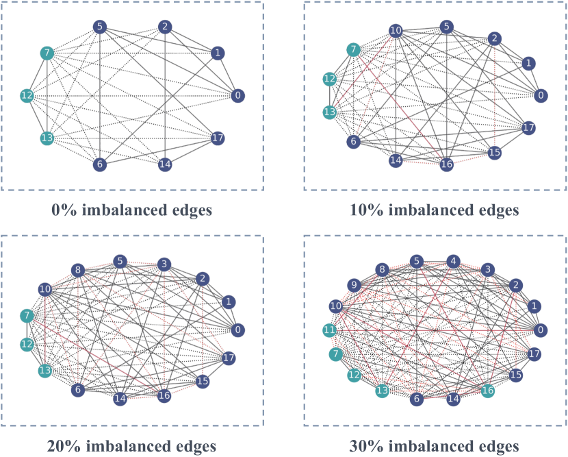
Figure 1. Balanced subgraphs are found in Cloister with different tolerance, where solid edges are positive, dashed edges are negative, black edges are balanced, and red edges are imbalanced.

There are two lines of work when studying social network polarization with signed graphs. Since most graphs coming from real scenarios are not balanced, if we can find the maximum balanced subgraph (MBS) instead, it usually reveals the largest polarized communities along with several important properties.

On the other line of work, instead of extracting the maximal subgraph, it focuses on removing edges to guarantee the balance of the original graph. The minimum number of edges whose deletion makes all connected components balanced is called the Frustration Index of the given signed graph.

However, such a notion of balance is strict in that no edge can disobey the condition. In reality, such strictness does not usually appear. For example, though being dominated, there usually exists some voices of disagreement on the majority idea, even in the most extreme community. Besides, two individuals in different political parties might reach a consensus on certain issues. In other words, there usually exist some imbalanced edges in signed graphs extracted from the community, which are against the strict notion of balance. Failing to handle these imbalanced edges might prevent us from identifying, extracting, and characterizing the community properly in real scenarios. We provide an example in Figure 1: As we increase the limitation for imbalanced edges, the community is getting significantly larger and denser. Therefore, we may be unable to capture the actual community if we prohibit imbalanced edges when computing.

Many questions arise here due to the many limitations:

• Can these two lines of work be unified?

• Can we develop algorithms finding communities that are non-strictly balanced?

In this paper, we answer these questions affirmatively. We design a tailored function to measure the tolerance of the imbalance. To properly describe such tolerance, we adapt the frustration index as part of the tolerance function. In this way, we can either allow no tolerance to extract the MBS in the network or a loose tolerance to extract communities that might contain voices of disagreement. We further raise new problems based on this tolerance model and present a new region-based heuristic algorithm that computes maximal balanced subgraphs under the tolerance setting. Our new algorithm is versatile, delivering high-quality solutions across a range of problems based on the tolerance model, and it’s also efficient, with an expected output time proportional to the size of the result. By setting different tolerances, we utilize our algorithm to handle different tasks and compare it with the performance of state-of-the-art algorithms on 8 real-world datasets.

Our contributions are summarized as follows:

• We introduce a novel, generalized, and practical model for identifying balanced subgraphs with tolerance in signed graphs.

• We have developed an efficient region-based heuristic randomized algorithm, characterized by an expected time complexity proportional to the size of the output, and coupled with a guarantee of result quality.

• Extensive experiments show that our algorithm consistently outperforms the baselines in terms of the quality of the returned subgraphs and achieves up to 100$\times$ speedup in terms of running time.

• The effectiveness of our algorithm is also evident in its application to polarized community detection, as detailed in Section 5.5.

Outline. The rest of the paper is organized as follows. We review the related work in Section 2, and introduce our generalized maximum balanced subgraph model with tolerance in Section 3. Section 4 presents our region-based heuristic algorithm. Experimental results are given in Section 5, and we conclude in Section 6.

2. RELATED WORK

Signed Graphs

Signed graphs were first introduced by Harary in 1956 to study the notion of balance (Harary, 1953). Cartwright and Harary generalized Heider’s theory of balance onto signed graphs (Cartwright and Harary, 1956). Harary also developed an algorithm to detect balance in signed graphs (Harary and Kabell, 1980). There are other works on studying the minimum number of sign changes to make the graph balance (Akiyama et al., 1981). Spectral properties have also been studied recently. Hou et al. have studied the smallest eigenvalue in signed graphs’ Laplacian (Hou et al., 2003; Hou, 2005).

Many works focus on community detection or partition in signed graphs. Anchuri et al. give a spectral method that partitions the signed graph into non-overlapping balanced communities (Anchuri and Magdon-Ismail, 2012). Doreian and Mrvar propose an algorithm for partitioning a directed signed graph and minimizing a measure of imbalance (Doreian and Mrvar, 1996). Yang et al. give a random-walk-based method to partition into cohesively polarized communities (Yang et al., 2007). The more recent work is by Niu et al (Niu and Sarıyüce, 2023). They leverage the balanced triangles, which model cohesion and polarization simultaneously, to design a good heuristic.

Maximum Balanced Subgraphs

The Maximum Balanced Subgraphs (MBS) problem has two variants: maximizing the number of vertices (MBS-V) and edges (MBS-E). Poljak et al. give a tight lower bound in 1986 (Poljak and Turzík, 1986) on the number of edges and vertices of the balanced subgraph. the MBS-E problem is in fact NP-hard since it can be formulated as a generalization of the standard MaxCut problem. To find the exact solution, there are some algorithms in the context of fixed-parameter tractability (FPT) are developed (Hüffner et al., 2007; Crowston et al., 2013). More studies are on extracting large balanced subgraphs. DasGupta et al. have developed an algorithm based on semidefinite programming relaxation (SDP) (DasGupta et al., 2007). For the MBS-V problem, Figueiredo and Frota propose several heuristic methods in 2014 (Figueiredo and Frota, 2014).

In 2020, Ordozgoiti et al. proposed a new algorithm named Timbal (Ordozgoiti et al., 2020) that extracts large balanced subgraphs regarding both vertices and edges. Timbal relies on signed spectral theory and the bound for perturbations of the graph Laplacian. However, Timbal is not stable and the balanced subgraph it found is sometimes small and unsatisfying as shown in our experiments.

Frustration Index

The frustration index is first introduced in 1950s (Abelson and Rosenberg, 1958; Harary, 1959). Computing the frustration index is related to the EdgeBipartization problem, which requires minimization of the number of edges whose deletion makes the graph bipartite. Since EdgeBipartization is NP-hard, computing the frustration index is also NP-hard. The MaxCut is also a special case of the frustration index problem. Assuming Khot’s unique games conjecture (Khot, 2002), it is still NP-hard to approximate within any constant factor. For the non-constant factor case, there are works that produce a solution approximated to a factor of $O(\sqrt{\log n})$ (Agarwal et al., 2005) or $O(\log k)$ (Avidor and Langberg, 2007) where $n$ is the number of vertices and $k$ is the frustration index. Coleman et al. have given a review on different approximation algorithms (Coleman et al., 2008). Hüffner et al. show that the frustration index is fixed parameter tractable and can be computed in $O(2^{k}m^{2})$, where $m$ is the number of edges and $k$ is the fixed parameter (the frustration index) (Hüffner et al., 2010). There are also algorithms using binary programming models to compute the exact frustration index (Aref et al., 2018, 2020).

3. Problem Specification

A signed graph is an undirected simple graph $G=(V,E^{+},E^{-})$ where $V$ is the vertex set and $E^{+},E^{-}$ represent the positive and negative signed edge sets. We first give the formal definition of balanced graphs as follows, which is the same as the previous works (Ordozgoiti et al., 2020; Niu and Sarıyüce, 2023). Note that we and these works require the graph to be connected for the community detection proposal.

Definition 3.1 (Balanced Graph).

Given a signed graph $G=(V,E^{+},E^{-})$, $G$ is balanced if $G$ is connected and there exists a partition $V=V_{1}\cup V_{2},V_{1}\cap V_{2}=\emptyset$ such that for each edge $(i,j)\in E^{+}$, vertices $i$ and $j$ belong to the same set within $V_{1}$ and $V_{2}$, while for each edge $(i,j)\in E^{-}$, they belong to the different sets.

Graphs are usually not balanced, especially when they are from practical scenarios. Therefore, people turn to study to find the maximum balanced subgraph (MBS) from the given graph. There are usually two variants of problems: maximizing the number of vertices (Ordozgoiti et al., 2020) and edges (DasGupta et al., 2007).

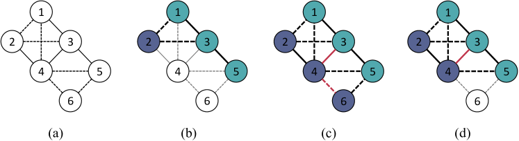
Figure 2. A signed graph (a), its MBS-V and MBS-E (b), its TMBS-V and TMBS-E (c), and its $\beta$-TMBS (d) with $\beta=\frac{1}{3}$.

We illustrate the concepts of MBS-V and MBS-E with an example in Figure 2, along with other problems to be discussed below. Here, we give a graph with 6 vertices numbered from $1$ to $6$ where solid edges are positive and dashed edges are negative, presented in (a). When solving Problem 1 or  2 on this graph, the optimal subgraph is constructed by vertex $1,2,3,5$, where $V_{1}=\{1,3,5\}$ and $V_{2}=\{2\}$. They are painted in two different colors in (b).

Another well-known problem in this topic is computing the minimum number of edges whose deletion makes all connected components balanced. This minimum amount of the edge removal is called the Frustration Index of the given signed graph $G$, denoted as $L(G)$.

Now, we are ready to introduce the concept of Balance with $\beta$-tolerance in signed networks, which is central to our paper.

Definition 3.2 (Balanced Graph under $\beta$-Tolerance).

Given a signed graph $G=(V,E^{+},E^{-})$ and a tolerance parameter $\beta\in(0,1]$, $G$ is balanced under $\beta$-Tolerance if $G$ is connected and $\frac{L(G)}{|E^{\prime+}\cup E^{\prime-}|}\leq\beta$.

In other words, when a graph is balanced under $\beta$-tolerance, it implies that by removing at most $\beta|E^{+}\cup E^{-}|$ edges from it, we can ensure that all connected components of the remaining graph become strictly balanced. Expanding upon the original definition of balance, this concept allows for the tolerance of a maximum of $\beta|E^{+}\cup E^{-}|$ edges that disobey the partitioning of polarized communities.

Under such $\beta$-tolerance restriction, finding the maximum balanced subgraph is generalized into the following two problems.

When $\beta$ becomes any value between $(0,\frac{1}{|E^{+}\cup E^{-}|})$, Problem 3 and Problem 4 are equivalent to the Problem 1 and Problem 2 respectively. However, unlike the strictly balanced graph, even deciding whether a signed graph satisfies $\beta$-tolerance is hard. Formally, we have the following lemma. The proof is deferred to Appendix A.1.

Lemma 3.1.

Given a signed graph $G=(V,E^{+},E^{-})$, deciding whether $G$ is balanced under $\beta$-tolerance cannot be done within polynomial time for tolerance parameter $\beta>\frac{1}{|E^{+}\cup E^{-}|}$, unless P $=$ NP.

Therefore, it is difficult to find large balanced graphs with tolerance and we cannot adapt any previous algorithms on MBS or other related problems. Meanwhile, there is another limitation that is worth mentioning. If $\beta\geq\frac{L(G)}{|E^{+}\cup E^{-}|}$, Problem 3 and Problem 4 has a trivial optimal solution: the largest connected component. That is to say, in such loose tolerance restriction, the optimal solution to these two problems might not reflect the polarized community. The previous showcase given in Figure 2 (c) is a typical example: When we solve Problem 3 and 4 with $\beta=\frac{1}{3}$ in such graph, we get the whole graph. However, vertex $6$ is in fact a noise that only has negative edges connected to both $V_{1}$ and $V_{2}$. Therefore, it should not be included in any meaningful subgraph solution.

To encounter the challenges and limitations, we first propose Tolerant Balance Index, a novel metric to evaluate signed graphs under the given tolerance for the balance.

Definition 3.3 (Tolerant Balance Index (TBI)).

Given a signed graph $G=(V,E^{+},E^{-})$ and a tolerance parameter $\beta\in(0,1]$, define its Tolerant Balance Index $\Phi(G,\beta)$ as the value of $|E^{+}\cup E^{-}|-\frac{L(G)}{\beta}$.

Correspondingly, we propose the following problem as the main task to solve throughout the paper.

It is easy to show, for any balanced graph $G$ under $\beta$-tolerance, $\Phi(G,\beta)\geq 0$. To discuss the usage of solving Problem 5, we also want to address that maximizing the number of edges (Problem 2 and 4) approximates the solution for maximizing the number of vertices (Problem 1 and 3). That is to say, these two variants of MBS problems are related.

Lemma 3.2.

Given a signed graph $G$, the solutions to Problem 2 and Problem 4 are $\frac{1}{\Delta}$-approximations for the Problem 1 and Problem 3 respectively, where $\Delta$ is the maximum degree of vertices in $G$.

We defer the proof of Lemma 3.2 to Appendix A.1. Considering the aforementioned interrelationship between two variants, we propose that finding the large connected subgraph with maximal $\Phi(G,\beta)$ (Problem 5) can be considered as a good approximation of the solutions to Problem 3 and Problem 4 simultaneously. In addition, since Problem 5 takes both the size and the polarity into account, it mitigates the limitation of large $\beta$. When we solve Problem 5 with $\beta=\frac{1}{3}$ on Figure 2 (a), the optimal subgraph will be vertices excluded vertex $6$, where $V_{1}=\{1,3,5\}$ and $V_{2}=\{2,4\}$, presented in (d). As it is shown, the noise vertex $6$ is not mistakenly selected into the optimal subgraph we try to find. Therefore, the polarity is being preserved.

In Section 4, we will present an efficient and effective algorithm for Problem 5. Then in Section 5, we will demonstrate the experimental results to support our proposal.

4. ALGORITHM

We propose Region-based Heuristic (RH), a new algorithm that searches for large balanced subgraphs with the $\beta$-tolerance restriction (Problem 5). Our algorithm runs in a given signed graph $G=(V,E^{+},E^{-})$, where $E^{+},E^{-}$ represent the positive and negative signed edge sets. The tolerance parameter $\beta$ is also given as input.

4.1. Relaxation

It is not easy to compute $\Phi(G,\beta)$ directly. Instead, we propose an alternative method to approximate it from the lower end while guaranteeing the tolerance condition ($\Phi(G,\beta)\geq 0$) is not violated.

For each vertex in $G$, we assign them with a color in $\{0,1\}$. Only vertices of the same color can be grouped in the same community. We denote any color assignment of $G$ as $\mathcal{X}$. Such definition is aligned with the previous work (Aref et al., 2020). Now, we are ready to give the formal definition of our newly proposed Tolerant Balanced Count.

Definition 4.1 (Tolerant Balance Count (TBC)).

Given a signed graph $G=(V,E^{+},E^{-})$ under coloring $\mathcal{X}$ and a tolerance parameter $\beta\in(0,1]$, define its Tolerant Balance Count as

$$\hat{\Phi}(G,\beta,\mathcal{X})=|E^{+}\cup E^{-}|-\frac{1}{\beta}\sum_{(i,j)\in E^{+}}\mathbbm{1}\{x_{i}\neq x_{j}\}-\frac{1}{\beta}\sum_{(i,j)\in E^{-}}\mathbbm{1}\{x_{i}=x_{j}\}$$

The following lemma states that $\Phi(G,\beta)$ is, in fact, the upper bound of $\hat{\Phi}(G,\beta,\mathcal{X})$ with respect to different coloring $\mathcal{X}$. The proof is deferred to Appendix A.2. We also have the following corollary that ensures the $\beta$-tolerance requirement is not violated.

Lemma 4.1.

Given a signed graph $G=(V,E^{+},E^{-})$ and a tolerance parameter $\beta\in(0,1]$, we have $\Phi(G,\beta)=\max_{\mathcal{X}}\hat{\Phi}(G,\beta,\mathcal{X})$.

Corollary 4.2.

Given a signed graph $G$ and a tolerance parameter $\beta$, $G$ is balanced under $\beta$-tolerance if there exists a coloring $\mathcal{X}$ such that $\hat{\Phi}(G,\beta,\mathcal{X})\geq 0$.

In this way, although we cannot compute $\Phi(G,\beta)$ directly, we can approximate the actual value by accumulating the non-negative $\hat{\Phi}(G,\beta,\mathcal{X})$ values of various coloring. Additionally, by Corollary 4.2, we can guarantee the $\beta$-tolerance during the whole computation. Such relaxation plays an important role in our algorithm, and the experimental results in Section 5 also validate its effectiveness.

4.2. Local Search

Our search process in Algorithm 1 starts from an initial vertex $s$ instead of the whole vertices set. We will discuss how to choose $s$ wisely in the later Section 4.3.

Search Operations

As discussed in Section 4.1, we will search for a connected subgraph $G^{\prime}$ and a coloring $\mathcal{X}$ that $\hat{\Phi}(G^{\prime},\beta,\mathcal{X})$ is as large as possible. In the following, if not specified, we use $\hat{\Phi}$ to denote the tolerant balanced count of the subgraph. Throughout the search process, we use a set $S$ to store the selected vertices and the coloring simultaneously. Specifically, $S$ stores selected tuples $(x,c)$, where $(x,c)$ represents a vertex $x$ colored as $c$. There are three basic operations with $S$ that will insert, delete, or change the color of a vertex $x$ respectively. Note that these three operations well define the neighborhood of any solution we find.

• $\texttt{VertexInsert}(x,c)$: Execute $S\leftarrow S\cup(x,c)$.

• $\texttt{VertexDelete}(x)$: Let $c$ be the color of $x$. Execute $S\leftarrow S\ \backslash\ (x,c)$.

• $\texttt{ColorFlip}(x)$: Let $c$ be the color of $x$ and $\overline{c}$ be $c$’s opposite color. Execute $\texttt{VertexDelete}(x)$ and $\texttt{VertexInsert}(x,\overline{c})$ in order.

Since our search begins from $s$, we initialize $S$ to be $\{(s,0)\}$ (line 1). We use $\hat{\Phi}_{opt}$ and $\hat{\Phi}_{cur}$ to store the maximum $\hat{\Phi}$ that we have found and the current $\hat{\Phi}$ respectively. Initially, they are initialized to be $0$ (line 1). During our process, if we choose to execute $\texttt{VertexInsert}(x,c)$ or $\texttt{ColorFlip}(x)$ for some vertex $x$, we will greedily execute one with the maximal increment of $\hat{\Phi}$ that it can contribute. Therefore, we use two max-heaps $MH_{I},MH_{F}$ to assist. After being initialized (line 1), since $s$ is selected, for each neighbor $v$ of $s$, we calculate the corresponding contribution to $\hat{\Phi}$ when $\texttt{VertexInsert}(v,0)$ or $\texttt{VertexInsert}(v,1)$ are executed and insert them to $MH_{I}$ (line 1 to  1). For $MH_{F}$, since only $s$ is selected, we calculate the contribution for $\texttt{ColorFlip}(x)$ and insert it into $MH_{F}$ (line 1).

Here, we do not use any structure to store the contribution when deleting any vertex from $S$. Instead, whenever we want to find the optimal deletion, we can compute for every vertex in $S$ altogether with a total cost of $O(n)$, which we may need to use the well-known Tarjan algorithm (Hopcroft and Tarjan, 1973) to guarantee the subgraph stays connected after the deletion. We denote such process as $\texttt{DelEval}(S)$.

Our search method is to execute one of the three operations repeatedly. If we only consider inserting vertices from $S$’s neighbors, the total number of VertexInsert is bounded by the size of the graph. However, since we also have the other two operations, which are non-incremental, if we do not design a proper termination strategy, the time complexity might become exponential. Specifically, we have two parameters that help to define the termination strategy of the algorithm: A float number $p\in(0,1)$ denotes the non-incremental probability and an integer $T$ to limit the number of potentially wasted operations.

Operation Selection

We first discuss how to select an operation each time. Here, we will use the non-incremental probability $p$ to help determine. We use $op$ to denote the operation we select and $\Delta_{\hat{\Phi}}$ to denote the corresponding contribution value to $\hat{\Phi}$. These two variables are initialized by acquiring the best VertexInsert operation from $MH_{I}$ (line 1), indicating choosing an insertion. Then, we generate a random float number $z$ from uniform distribution $U(0,1)$. If $z<p$, we also consider using a ColorFlip operation: We acquire the best ColorFlip operation from $MH_{F}$ and update the two variables if the corresponding $\Delta_{\hat{\Phi}}$ is larger than the current one (line 1 to  1). Similarly, we regenerate $z$ and if $z<\frac{p\log|S|}{|S|}$, we try choosing a VertexDelete operation: After calling $\texttt{DelEval}(S)$ to recalculate for every possible vertex deletion, we choose the best among them and try updating (line 1 to  1). In this way, we choose an VertexInsert operation by default, and with some probability, we check if the current optimal ColorFlip and VertexDelete can contribute more. The two probabilities are by design and help to balance between accuracy and efficiency.

We execute the current $op$ operation after the selection phase and also update the current $\hat{\Phi}_{cur}$. Since $S$ is updated after the execution, we must also update $MH_{I}$ and $MH_{F}$ correspondingly. This is done in a similar way as the initialization (line 1 to  1).

Search Termination

When the current selected operation enlarges the current $\hat{\Phi}_{cur}$, we denote such operation as a progressive one. Otherwise, it is non-progressive. We use a parameter $T$ to prevent too many non-progressive operations. Specifically, our search will terminate when the number of non-progressive operations exceeds $T$ times the number of progressive operations. We implement such a strategy with a counter $t$. After we select and execute an operation (line 1 to  1), we compare the current $\hat{\Phi}_{cur}$ with $\hat{\Phi}_{opt}$. If $\hat{\Phi}_{cur}$ is smaller, we decrease $t$ by $1$. Otherwise, we update $\hat{\Phi}_{opt}$ and increase $t$ by $T$ (line 1 to  1). In this way, if $t<0$, the search should terminate (line 1). In addition, we also terminate the search when $S$ contains all vertices in $G$ since no further insertion can be executed (line 1). After the search, we undo the last few non-progressive operations to retract the optimal subgraph we have found (line 1). We return with this subgraph as $\overline{H}$ and its corresponding $\hat{\Phi}$ (line 1).

Input: Signed graph $G$; Tolerance parameter $\beta$; Non-incremental probability $p$; Initial vertex $s$; Early stop turn limit $T$.

Output: $\overline{H}\subseteq G$: the found balanced subgraph with $\beta$-tolerance; $\hat{\Phi}$: the lower bound of $\overline{H}$’s balance value we achieved.

1 $S\leftarrow\{(s,0)\}$, $\hat{\Phi}_{opt}\leftarrow 0$, $\hat{\Phi}_{cur}\leftarrow 0$, $t\leftarrow T$;

2 Initialize max-heaps $MH_{I},MH_{F}$;

3 Insert $s$ into $MH_{F}$;

4 for $v\in N(s)$ do

5       Insert $(v,0)$ and $(v,1)$ into $MH_{I}$;

6

7while $t\geq 0\text{ and }|S|<|V(G)|$ do

       $\{op,\Delta_{\hat{\Phi}}\}=\texttt{GetTopNode}(MH_{I})$;

        // ordered by $\Delta_{\hat{\Phi}}$

8       if $z\sim U(0,1)<p$ then

9             $\{op,\Delta_{\hat{\Phi}}\}\leftarrow\max(\{op,\Delta_{\hat{\Phi}}\},\texttt{GetTopNode}(MH_{F})$);

10      if $z\sim U(0,1)<\frac{p\log|S|}{|S|}$ then

11             $\{\hat{op},\overline{\Delta_{\hat{\Phi}}}\}\leftarrow$ DelEval$(S)$;

12             $\{op,\Delta_{\hat{\Phi}}\}\leftarrow\max(\{op,\Delta_{\hat{\Phi}}\},\{\hat{op},\overline{\Delta_{\hat{\Phi}}}\})$;

13      $S\leftarrow$ Execute operation $op$ on $S$;

14       $x\leftarrow$ the vertex of the $op$;

15       for $v\in N(x)\cup x$ do

16             Insert, update or delete $v$’s operations in $MH_{I}$ and $MH_{F}$;

17            

18      $\hat{\Phi}_{cur}\leftarrow\hat{\Phi}_{cur}+\Delta_{\hat{\Phi}}$;

19       if $\hat{\Phi}_{cur}\leq\hat{\Phi}_{opt}$ then $t\leftarrow t-1$;

20       else  $\hat{\Phi}_{opt}\leftarrow\hat{\Phi}_{cur}$, $t\leftarrow t+T$ ;

21      

22Undo the last non-progressive operations on $S$;

return $\overline{H}=G[S],\hat{\Phi}=\hat{\Phi}_{opt}$;

Algorithm 1 RH: Search

4.3. Region-based Sampling

In the previous section, we propose a search process that starts from an arbitrary vertex $s$. It is reasonable to foresee that the choice of $s$ might affect the result significantly. If we start only from too few vertices, our result in the end might be some local maximal solutions, which would be much worse than the global maximal one. One of the solutions is to enumerate all possible $s$, i.e., all vertices in $G$. However, such pure enumeration may result in excessively high time complexity. To balance between performance and efficiency, we propose a Region-based Sampling strategy.

Our sampling method is mainly based on two hypotheses. The first hypothesis indicates that the probability of finding a nearly optimal subgraph is high if we are able to select some vertices in the optimal subgraph as the starting vertex. Here, the ‘optimal’ denotes the solution we found by enumerating all vertices as the starting vertex. We formally state such a hypothesis as follows.

Hypothesis 4.1.

Given a signed graph $G$ and a tolerance parameter $\beta$, suppose the optimal subgraph found by Algorithm 1 starting with vertex $x$ is $G_{x}$, and the optimal graph among all $G_{x}$ is $G_{opt}$. For the given $\epsilon$, there exists a subset $V^{\prime}\subseteq V(G_{opt})$ with $\frac{|V^{\prime}|}{|V(G_{opt})|}\geq\frac{1}{2}$ such that $\Phi(G_{x},\beta)\geq(1-\epsilon)\Phi(G_{opt},\beta),\forall x\in V^{\prime}$.

Another hypothesis describes the relation between $\hat{\Phi}$ values returned by two different calls of Algorithm 1, if we select different starting vertex. We argue that if the return $\hat{\Phi}$ value is larger, the found subgraph will likely be bigger. We formally state such a hypothesis as follows.

Hypothesis 4.2.

Given a signed graph $G$ and a tolerance parameter $\beta$, suppose the optimal subgraph and coloring found by Algorithm 1 starting with vertex $a$ are $G_{a}$ and $\mathcal{X}_{a}$, starting with $b$ are $G_{b}$ and $\mathcal{X}_{b}$. If $\hat{\Phi}(G_{a},\beta,\mathcal{X}_{a})\geq\hat{\Phi}(G_{b},\beta,\mathcal{X}_{b})$, we have $|V(G_{b})|\leq 2|V(G_{a})|$.

With these two hypotheses, we have the following lemma that describes a sampling strategy that is able to find a $(1-\epsilon)$-optimal subgraph within an acceptable number of calls of the search process. The proof is deferred to Appendix A.2.

Lemma 4.3.

Given a signed graph $G$, a tolerance parameter $\beta$, and a positive $\epsilon<1$, suppose we run Algorithm 1 in $k$ iterations, where the $i$-th iteration starts with a uniformly sampled vertex $x_{i}\in V(G)$, and the optimal subgraph found is $G_{i}$. If Hypothesis 4.1 and Hypothesis 4.2 hold, the expected number of iterations that find a $(1-\epsilon)$-optimal subgraph $\mathbb{E}\left[X\right]$ is $\Omega(\sum_{i=1}^{k}|V(G_{i})|/|V(G)|)$.

Input: Signed graph $G$; Tolerance parameter $\beta$; Iteration constant $\mathcal{C}$; Non-incremental probability $p$; Early stop turn limit $T$.

Output: $H\subseteq G$: the found balanced subgraph with $\beta$-tolerance.

1 $H\leftarrow\emptyset$;

2 $\hat{\Phi}_{opt}\leftarrow 0$;

3 $TotalSize\leftarrow 0$;

4 while $TotalSize<\mathcal{C}|V(G)|$ do

5       $s\leftarrow$ Sample a vertex from $V(G)$;

6       $\overline{H},\hat{\Phi}\leftarrow$ Search($G,\beta,s,p,T$);

7       if $\hat{\Phi}>\Phi_{opt}$  then

8             $\hat{\Phi}\leftarrow\hat{\Phi}_{opt}$;

9             $H\leftarrow\overline{H}$;

10      $TotalSize\leftarrow TotalSize+|V(\overline{H})|$;

return $H$;

Algorithm 2 RH: Sampling

We provide an implementation of such sampling strategy in Algorithm 2, which is, in fact, an application of Lemma 4.3. We use $H$, $\hat{\Phi}_{opt}$ to keep track of the current optimal subgraph and its corresponding $\hat{\Phi}$ value. They are initialized to be $\emptyset$ and $0$ in the beginning (line 2 to  2). We also use a variable $TotalSize$ to keep track of the total size of all return subgraphs from Algorithm 1, which is also initialized to be $0$ (line 2).

For each iteration, we randomly select a vertex $s$ (line 2) as the starting vertex and pass it into Algorithm 1 (line 2). After receiving the result from Algorithm 1, we update $H$, $\hat{\Phi}_{opt}$ (line 2 to  2) if the newly found subgraph is better (line 2). Before the new iteration, we accumulate the size of the newly found subgraph into $TotalSize$ (line 2. The whole process will stop when $TotalSize\geq\mathcal{C}|V(G)|$ (line 2). By Lemma 4.3, we can set a proper termination condition by accumulating the subgraph size from each search process. More specifically, When $TotalSize$ reaches $\mathcal{C}|V(G)|$, it is expected to find a nearly optimal solution $\mathcal{C}$ times. In the end, we return $H$ as the main result (line 2).

Time Complexity Analysis

We show that the time complexity of Algorithm 2 is $O(\Delta(\mathcal{C}+1)n\log^{2}n)$, where $n$ is the number of vertices in $G$. We start with the time complexity of Algorithm 1.

Lemma 4.4.

Suppose that the loop starting on Line 1 repeats for a total of $t$ times. Let $h$ be the size of $S$ on Line 1. Then we have, with high probability, $h=\Omega(t/\log n)$ and that the running time of Algorithm 1 is $O(\Delta t\log n)$ in expectation.

Proof.

By Lemma A.1, with high probability, $h=\Omega(t/\log n)$.

Let $\Delta$ be the maximum degree of $G$. The running time of each iteration is dominated by the cost of updating the heaps and the time for DelEval($S$). Updating the heaps cost $O(\Delta\log n)$ time. The function DelEval($S$) costs $O(\Delta|S|)$ time. It is called with probability $\frac{p\log|S|}{|S|}$ in each iteration. Thus, its expected runtime in each iteration is $O(\Delta\log n)$. We have the running time of Algorithm 1 is $t\cdot O(\Delta\log n)=O(\Delta t\log n).$ ∎

Lemma 4.5.

With high probability, the expected time complexity of Algorithm 2 is $O(\Delta(\mathcal{C}+1)n\log^{2}n)$.

Proof.

Suppose we call Line 2 for $k$ times. For the $i$-th call, let $t_{i}$ be the number of iterations of the loop on Line 1 and let $h_{i}$ ($1\leq i\leq k$) be the size of $S$ on Line 1. By Lemma 4.4, the total time complexity in expectation is $O(\sum_{i=1}^{k}\Delta t_{i}\log n)$, and the sum of $h_{i}$ satisfies $\sum_{i=1}^{k}h_{i}=\Omega(\sum_{i=1}^{k}t_{i}/\log n).$ Since $\sum_{i=1}^{k}h_{i}\leq(\mathcal{C}+1)n$, we have that the total runtime of Algorithm 2 in expectation is $O(\sum_{i=1}^{k}\Delta t_{i}\log n)=O(\Delta(\mathcal{C}+1)n\log^{2}n)$. ∎

5. EVALUATION

In this section, we address the following research questions to evaluate various important aspects of our algorithm:

• RQ1 (Effectiveness - TMBS): Given various $\beta$, what are the optimal subgraphs in terms of size, and Tolerant Index Count, found by our method and baselines?

• RQ2 (Effectiveness - MBS): What are our method’s and baselines’ performances in finding the maximal balanced subgraph?

• RQ3 (Efficiency): What are the runtimes for our method and the baselines, and how do they scale with very large networks?

• RQ4 (Generalizability): Can our model and method be adapted to other related tasks in the signed networks?

We also conduct three experiments shown in appendix B, which are designed to validate our hypotheses, determine optimal hyperparameters, and assess stability.

5.1. Experimental Setting

Baselines

We compare our method with the baselines from highly related works (e.g., MBS and polarized community detection), including spectral and other heuristic methods.

Note that since finding tolerant balanced subgraphs is typically more challenging than previous community detection tasks in signed networks, we also adapt our TBC-relaxation in Section 4.1 for all baseline methods to ensure that they can return the subgraphs satisfying the tolerance constraint. We summarize the core ideas of each baseline method as follows.

• Eigen: Based on a spectral method from (Bonchi et al., 2019), we first compute $\mathbf{v}$, the eigenvector of the signed adjacency matrix $A$ corresponding to the largest eigen value $\lambda$. For each vertex $i$, if a Bernoulli experiment with success probability $p=|\mathbf{v}_{i}|$ is successful, we assign vertex $i$ a color determined by $\text{sgn}(\mathbf{v}_{i})$. The maximum connected components with non-negative $\hat{\Phi}$ serve as solutions to Problem 3 and Problem 4, while the connected component with the maximum $\hat{\Phi}$ provides the solution to Problem 5.

• Timbal: Based on a state-of-the-art method for MBS from (Ordozgoiti et al., 2020), we start from the entire graph and repeatedly remove vertices from it, guided by an eigenvalue approximation outlined in their paper. Specifically, we compute $\hat{\Phi}$ by the optimal coloring among two non-trivial methods (Bonchi et al., 2019; Gülpinar et al., 2004) for TMBS problems.

• GreSt: This method combines a classical and effective algorithm in dense subgraph (Charikar, 2000) and a heuristic coloring method for signed networks by spanning tree (Gülpinar et al., 2004). Firstly, we determine the coloring of the entire graph by a random spanning tree. We then repeatedly remove vertices maximizing $\hat{\Phi}$ of the remaining graph. A min-heap is used to speed up the process of finding vertices. To acquire the solution to different tasks, we need to store the deletion operations. Then we can restore the graph by undoing deletions one by one. Such reversal allows us to keep track of the optimal connected component efficiently, instead of scanning the whole graph after each deletion.

• RH (LS): Instead of using region-based sampling, we execute our local search in Section 4.2 for all starting vertices and select the optimal solutions, to investigate the effectiveness of the regional-based sampling. This method may provide a better solution than RH but is not efficient.

Table 1. Signed network datasets used in experiments, including the number of vertices ($|V|$) and edges ($|E|$), the ratio of negative edges ($\rho^{-}$), and the ratio of non-zero elements ($\delta$).

Dataset	$|V|$	$|E^{+}\cup E^{-}|$	$\rho^{-}=\frac{|E^{-}|}{|E^{+}\cup E^{-}|}$	$\delta=\frac{2|E^{+}\cup E^{-}|}{|V|(|V|-1)}$
Bitcoin	5k	21k	0.15	1.2e-03
Epinions	131k	711k	0.17	8.2e-05
Slashdot	82k	500k	0.23	1.4e-04
Twitter	10k	251k	0.05	4.2e-03
Conflict	116k	2M	0.62	2.9e-04
Elections	7k	100k	0.22	3.9e-03
Politics	138k	715k	0.12	7.4e-05
Growth	1.87M	40M	0.50	2.3e-05

Datasets

We select 7 publicly-available real-world signed networks, Bitcoin, Epinions, Slashdot, Twitter, Conflict, Elections, and Politics, which were widely used in previous related works (Ordozgoiti et al., 2020; Bonchi et al., 2019; Niu and Sarıyüce, 2023). In addition, to investigate our methods’ scalability, we generate Growth, a very large signed network induced from the real temporal network Wikipedia-growth. Specifically, we select a threshold $\tau$, and give positive signs for the edges with time stamp $t(e)\geq\tau$ and negative signs for the edges with $t(e)<\tau$. By using a proper $\tau$, the ratio of negative edges of the induced graph can be $0.5$. In this network, a balanced graph contains two communities, where the edges within each community are recently formed, while the crossing edges are relatively old. Detailed information for each dataset can be found in Table 1.

All experiments are conducted on a Ubuntu 22.04 LTS workstation, equipped with a 12th Gen Intel(R) Core(TM) i9-12900HX. We set hyperparameters $T=20,p=0.8,\mathcal{C}=1.5$ for all experiments.

5.2. Finding Balanced Subgraphs with Tolerance

We aim to identify sizable and polarized subgraphs while taking the tolerance into account (RQ1). Firstly, by running algorithms in Section 5.1, we keep track of the optimal subgraph that we have found to Problem 3, Problem 4, and Problem 5 respectively. Noticeably, we do not modify either RH or RH (LS) for Problem 3 and Problem 4. That is to say, we directly use our result on solving Problem 5 to compare with other algorithms which are tailored for either Problem 3 or Problem 4, which demonstrates our proposed Problem 5 is a good approximation for the other two problems.

The comparison results for these three problems are shown in Figure 3, Figure 4, and Figure 5, respectively. In our experiments, we consider $15$ different tolerance parameters ($\beta_{i}=2^{-i/2}$ for all $2\leq i\leq 16$), where $i=2$ implies allowance for all connected subgraphs, while $i=16$ means that the found subgraphs are almost strictly balanced. Since Problem 3 and Problem 4 become trivial when $\beta\geq\frac{L(G)}{|E^{+}\cup E^{-}|}$, we shade the corresponding ranges in Figure 3 and Figure 4. We omit the results for methods that cannot finish in 100,000 seconds.

Observing the experiment results, our proposed method RH outperforms all other baselines significantly in all three problems. This also demonstrates that our proposed tolerance model is a more realistic model for the general case of balanced signed graph models. In addition, we can see that RH produces results that are close to RH (LS). Therefore, we manage to empirically support our hypothesis in Section 4.3 in real-world data.

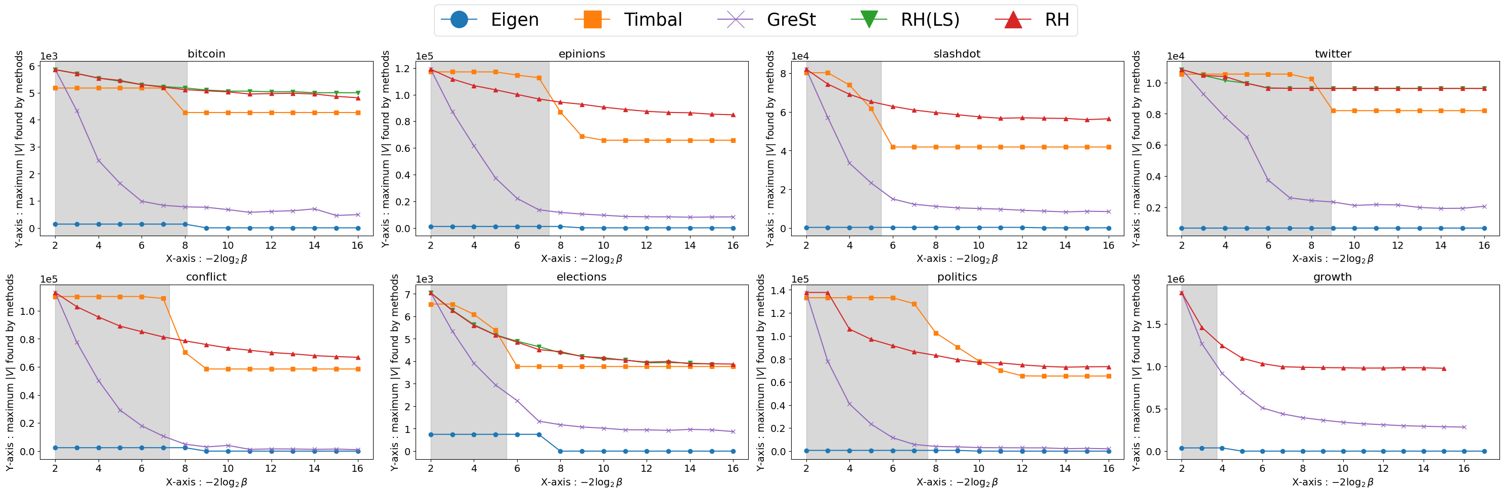
Figure 3. Problem 3: Comparing maximum tolerantly balanced subgraphs in vertex cardinality ($|V|$) across various tolerances ($\beta=2^{-x/2}$), where the part corresponding to trivial $\beta$ values for this problem has been shaded.

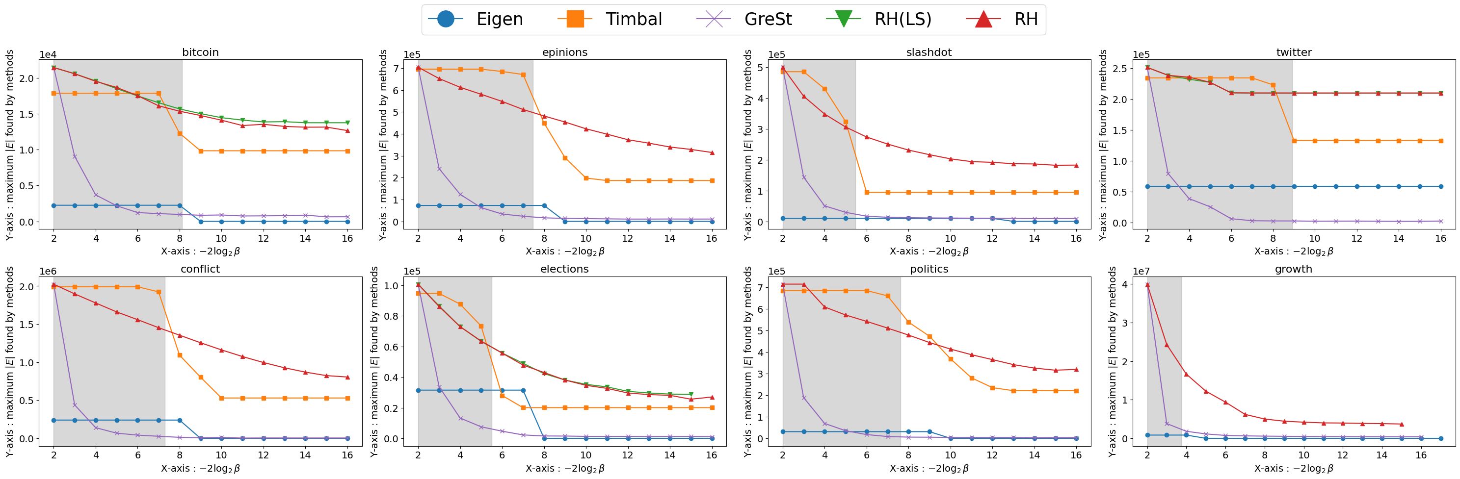
Figure 4. Probelm 4: Comparing maximum tolerantly balanced subgraphs in edge cardinality ($|E^{+}\cup E^{-}|$) across various tolerances ($\beta=2^{-x/2}$), where the part corresponding to trivial $\beta$ values for this problem has been shaded.

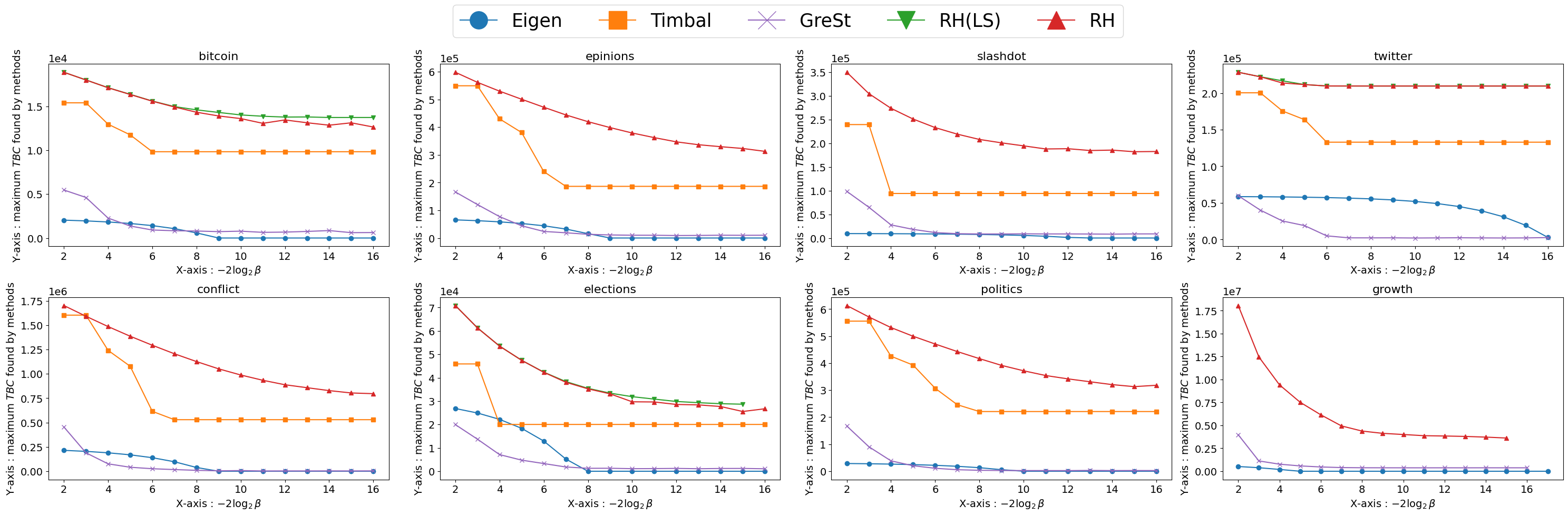
Figure 5. Probelm 5: Comparing maximum tolerantly balanced subgraphs in TBC ($\hat{\Phi}$) across various tolerances ($\beta=2^{-x/2}$).

5.3. Finding Strictly Balanced Subgraphs

Finding the Maximum Balanced Subgraph (Problem 1 and  2) is an important and well-studied problem in signed networks (Ordozgoiti et al., 2020) (RQ2). As previously discussed, MBS problems are special forms of proposed TMBS problems (Problem 3 and  4) by setting $\beta<\frac{1}{|E^{+}\cup E^{-}|}$.

Table 2 shows the results of our case study on the MBS problems, where we omit the results for Eigen since it can not return subgraphs other than a single vertex. RH produces significantly better results than the previous state-of-the-art method Timbal, which is specifically designed for the MBS problems while ours is not.

Table 2. Case study: Largest strictly balanced subgraph (in terms of $|V|$ or $|E|$) found by each method for each dataset ($\beta<\frac{1}{|E^{+}\cup E^{-}|}$), where NA denotes the corresponding method cannot finish in 100,000 seconds on the respective dataset.

Method	Bitcoin		Epinions		Slashdot		Twitter		Conflict		Elections		Politics		Growth
	$|V|$	$|E|$	$|V|$	$|E|$	$|V|$	$|E|$	$|V|$	$|E|$	$|V|$	$|E|$	$|V|$	$|E|$	$|V|$	$|E|$	$|V|$	$|E|$
Timbal	4,050	9,757	65,879	190,751	43,742	101,590	8,636	129,927	51,463	361,663	3,579	17,633	65,188	230,529	NA	NA
GreSt	571	713	7,078	9,229	7,923	8,465	1,895	2,277	759	4,885	935	1,232	2,371	3,155	272,621	375,603
RH (LS)	5,002	13,746	NA	NA	NA	NA	9,628	209,633	NA	NA	3,970	28,453	NA	NA	NA	NA
RH	4,935	13,050	84,165	302,152	55,968	181,069	9,628	209,633	65,468	746,640	3,926	26,478	72,431	317,384	999,504	3,415,441

5.4. Running Time Analysis

This experiment is designed to study the efficiency and scalability of our method (RQ3). As shown in Table 3, when the graph size is up to ($|V|=1.87$M, $|E^{+}\cup E^{-}|=40$M), RH can still produce reasonable results within 1,000 seconds. On the other hand, the other four compared methods either produce much worse results while taking longer time or even fail to finish execution in 100,000 seconds. In all, the empirical results demonstrate the efficiency of our method in real-world data in addition to its asymptotic theoretical complexity.

Table 3. Mean running time (s) for each method on the various $\beta$ in Section 5.2.

Dataset	Eigen	Timbal	GreSt	RH (LS)	RH
Bitcoin	0.979	2.670	0.018	135.040	0.057
Epinions	9.213	220.919	0.319	$\geq 100,000$	4.162
Slashdot	7.287	226.805	0.218	$\geq 100,000$	3.175
Twitter	1.704	7.306	0.085	2,516.671	0.493
Conflict	12.899	310.736	0.781	$\geq 100,000$	9.031
Elections	1.022	4.542	0.039	675.484	0.288
Politics	10.003	143.605	0.304	$\geq 100,000$	4.782
Growth	297.299	$\geq 100,000$	48.915	$\geq 100,000$	813.099

5.5. Solving the 2PC Problem

This experiment aims to evaluate the generalizability when adapting RH and our tolerant model to different variants of polarity community detection (RQ4). In addition to balance-related problems, 2-Polarized-Communities (2PC), proposed by Bonchi and Galimberti (Bonchi et al., 2019), serves as another model for polarized community detection. In their model, the measurement of polarity is penalized by the size of the solution:

To solve the 2PC problem by our tolerance balance model, we add an additional penalty term to the solution size in the tolerant balance count: We define $\hat{\Phi}^{\prime}(G,\beta,\mathcal{X},\rho)=\hat{\Phi}(G,\beta,\mathcal{X})-\rho|V|$ to serve as a new object function in our RH algorithm. Throughout the algorithm, we set $\beta=\frac{1}{2}$. This is because when $\beta=\frac{1}{2}$, if $\hat{\Phi}^{\prime}\geq 0$, the polarity is no less than $\rho$. Therefore, Problem 6 can be solved by the new RH algorithm, where we apply an iterative mechanism on $\rho$. The algorithm details can be found in Appendix A.3.

We compare RH’s results with the optimal result computed by the two methods in Bonchi and Galimberti’s paper (Bonchi et al., 2019) (i.e., Eigen and Greedy). The results are shown in Table 4. RH’s slight modifications efficiently yield promising communities, demonstrating the adaptability and effectiveness of our tolerant balance model and algorithm in varied polarity community detection scenarios.

Table 4. Optimal subgraphs in the term of 2PC-polarity ($\frac{x^{T}Ax}{x^{T}x}$) found by each method, associated with running time.

Dataset	RH		Eigen		Greedy
	polarity	time (s)	polarity	time (s)	polarity	time (s)
Bitcoin	14.82	0.035	14.76	0.706	14.50	0.999
Epinions	85.27	0.873	64.36	10.271	85.15	428.625
Slashdot	41.21	0.584	39.85	7.325	41.36	154.383
Twitter	87.21	0.818	87.04	1.717	86.97	7.853
Conflict	94.27	15.134	87.83	13.144	63.99	552.629
Elections	36.27	0.395	35.87	0.950	36.34	2.223
Politics	44.95	0.862	44.22	9.931	45.01	475.353

6. CONCLUSIONS

This paper presents a new and versatile model to identify polarized communities in signed graphs. The model accommodates inherent imbalances in polarized communities through a tolerance feature. Additionally, we propose a region-based heuristic algorithm. Through a wide variety of experiments on graphs of up to 40 M edges, it demonstrates effectiveness and efficiency beyond the state-of-the-art methods in addressing both traditional and generalized MBS problems. We also adapt our model and algorithm to 2PC, a related but essentially different task, further verifying their generalizability.

Appendix A OMITTED PROOF AND ALGORITHM

A.1. Omitted Proof in Section 3

Proof of lemma 3.1.

We prove the lemma by a reduction from the calculation of the Frustration Index. If we can decide whether $G$ is balanced under $\beta$-tolerance within the polynomial runtime, we will be able to decide whether $L(G)$ is greater than any guessing value $k$ by setting $\beta=\frac{k}{|E^{+}\cup E^{-}|}$. Combined with a binary search, we can compute the Frustration Index of $G$ within the polynomial runtime, which has been proven as a NP-hard problem (Agarwal et al., 2005). ∎

Proof of lemma 3.2.

We first show that the solutions to Problem 2 is a $\frac{1}{\Delta}$-approximations for the Problem 1, and the relations between Problem 3 and Problem 4 can be proven similarly.

Given a signed graph $G$, let the optimal subgraph to Problem 1 be $G_{1}$ with $n_{1}$ vertices and $m_{1}$ edges, and the optimal subgraph to Problem 2 be $G_{2}$ with $n_{2}$ vertices and $m_{2}$ edges. Since $G_{1}$ is connected, we have

(1) $$m_{1}\geq n_{1}$$

Since $\Delta$ is the maximum degree of vertices in $G$, we have

(2) $$n_{2}\geq\frac{m_{2}}{\Delta}$$

Combined with (1) and (2), we have $n_{2}\geq\frac{m_{2}}{\Delta}\geq\frac{m_{1}}{\Delta}\geq\frac{n_{1}}{\Delta}$, which implies $G_{2}$ is a $\frac{1}{\Delta}$-approximations for the Problem 1. ∎

A.2. Omitted Lemma and Proof in Section 4

Proof of lemma 4.1.

The lemma is equivalent to that:

$\sum_{(i,j)\in E^{+}}\mathbbm{1}\{x_{i}\neq x_{j}\}+\sum_{(i,j)\in E^{-}}\mathbbm{1}\{x_{i}=x_{j}\}$ is a tight upper bound on $L(G)$.

First, given a coloring $\mathcal{X}$, if we remove all edges that let the indicator functions be true from $G$, the remaining graph will be balanced for each connected component due to Definition 3.1. This implies that $\sum_{(i,j)\in E^{+}}\mathbbm{1}\{x_{i}\neq x_{j}\}+\sum_{(i,j)\in E^{-}}\mathbbm{1}\{x_{i}=x_{j}\}$ is no less than the $L(G)$, which is the minimum number of edges to be removed.

We then show the bound is tight. Consider the remaining graph $G^{\prime}$ from removing all edges contributing to $L(G)$. Since all connected components of $G^{\prime}$ are balanced, we can find a partition $V=V_{1}\cup V_{2}$ and $V_{1}\neq V_{2}$ such that if we assign $x_{i}=0$ for all $i\in V_{1}$ and $x_{j}=1$ for all $j\in V_{2}$, the value of $\sum_{(i,j)\in E^{+}}\mathbbm{1}\{x_{i}\neq x_{j}\}+\sum_{(i,j)\in E^{-}}\mathbbm{1}\{x_{i}=x_{j}\}$ will become to zero for $G^{\prime}$. This implies the same value for $G$ under the coloring is equal to $L(G)$ and thus the bound is tight. ∎

Proof of lemma 4.3.

Suppose the optimal subgraph found by Algorithm 1 among all starting vertex is $G_{opt}$ and the probability of Algorithm 2 finding a $(1-\epsilon)$-optimal subgraph in one iteration is $\Pr[\text{Sucess}]$. By Hypothesis 4.1, we have (i) $\Pr[\text{Sucess}]\geq\frac{|V(G_{opt})|}{2|V(G)|}$. Let $\mathcal{C}=\frac{\sum_{i=1}^{k}|V(G_{i})|}{|V(G)|}$, and then we have $\sum_{i=1}^{k}|V(G_{i})|=\mathcal{C}|V(G)|$. By Hypothesis 4.2, $\sum_{i=1}^{k}2|V(G_{opt})|\geq\mathcal{C}|V(G)|$, and thus (ii) $k\geq\frac{\mathcal{C}}{2}\frac{|V(G)|}{|V{(G_{opt})}|}$. Combining (i) and (ii), we have $\mathbb{E}\left[X\right]=k\Pr[\text{Sucess}]\geq\frac{\mathcal{C}}{2}\frac{|V(G)|}{|V{(G_{opt})}|}\cdot\frac{|V(G_{opt})|}{2|V(G)|}=\frac{\mathcal{C}}{4}=\Omega(\mathcal{C})$. ∎

Lemma A.1.

With high probability, for all valid $i$, after the $i$-th iteration of the on Line 1 of Algorithm 1, $|S|=\Omega(\frac{i}{\log n})$.

Proof.

Let $x$ denote the value of $|S|$. The initial value of $x$ is $1$. $x$ changes according to the following rules in each iteration:

• With probability $(1-p)(1-p\frac{\log x}{x})$, $x$ increases by $1$;

• With probability $p\frac{\log x}{x}$, x increases by $1$, $0$, or $-1$;

• With probability $p(1-p\frac{\log x}{x})$, x increases by $1$, or $0$;

• The process ends when $x$ reaches $n$.

Suppose the process lasts for $t$ steps. It suffices to prove that with high probability, it holds simultaneously for all $i$ from $1$ to $t$ that the value of $x$ after the first $i$ steps is $\Omega(\frac{i}{\log n})$.

We denote $(1-p)(1-p\frac{x}{\log x})$ by $p^{+}(x)$, $p(1-p\frac{x}{\log x})$ by $p^{0}(x)$, and $p\frac{x}{\log x}$ by $p^{-}(x)$.

Let $next(x)$ be the value of $x$ in the next step.

Let $x_{0}$ be the smallest $x$ such that $p^{-}(x)<p^{+}(x)/2$. Such $x_{0}$ exists because $p^{-}(x)\rightarrow 0$ and $p^{+}(x)\rightarrow 1-p$ when $x\rightarrow\infty$. For any $x\geq x_{0}$, $\mathbb{E}\left[next(x)\right]\geq x+\frac{1-p}{3-p}.$

We have that $x_{0}$ is a constant depending on $p$. Let $c$ be the maximum expected number of steps for the variable $x$ to reach $x_{0}$ from any initial value $x_{init}<x_{0}$. $c$ is a constant depending on $p$.

By Markov bound, we have that in every $2c$ steps, with probability at least $1/2$, there exists at least one step before which $x$ is at least $x_{0}$. Thus, in $k=\Omega(\log n)$ steps, with high probability, there exists $\Omega(k)$ steps before which the value of $x$ is at least $x_{0}$.

In these $\Omega(k)$ steps, $x$ increases by expectation value at least $\frac{1-p}{3-p}\Omega(k)=\Omega(k)$. The rest of the $k$ steps can be partitioned into consecutive segments. In each segment, $x$ increases from some value less than $x_{0}$ to $x_{0}$. The only exception is the last segment where $x$ may decrease by at most $x_{0}$. Thus, in expectation, after the $k$ steps, the value of $x$ is at least $\Omega(k).$

We may repeat the argument above for $O(\log n)$ rounds to boost the probability. After $\Omega(k\log n)$ steps, the value of $x$ is $\Omega(k)$ with high probability.

By plugging in $k=n$, we have that the process ends in $t=O(n\log n)$ steps with high probability. By a union bound, we can prove that the value of $x$ after the first $i$ steps being $\Omega(i/\log n)$ holds simultaneously for all $i$ from $1$ to $t$ with high probability. ∎

A.3. Omitted Algorithm in Section 5.5

Input: Signed graph $G$;

Output: $H\subseteq G$: the found subgraph with high 2PC polarity; $\rho:$ the 2PC polarity of $H$;

1 $H\leftarrow\emptyset$; $\rho\leftarrow 0$;

2 $s\leftarrow$ Sample a vertex from $V(G)$;

3 while true do

       $\overline{H},\hat{\rho}\leftarrow$ Search($G,\beta=\frac{1}{2},\sigma=0.9\rho,s$);

        // guided by the new object function $\hat{\Phi}^{\prime}=\hat{\Phi}-\sigma|S|$. hyperparameters $T$ and $p$ are omitted.

4       if $\hat{\rho}>\rho$ then

5             $\rho\leftarrow\hat{\rho}$;

6             $H\leftarrow\overline{H}$;

7      else  $s\leftarrow$ Sample a vertex from $V(G)$ ;

8       if meets stop-conditions then break;

9       remove all vertice with degree less than $\rho$ from $G$;

return $H,\rho$;

Algorithm 3 RH: Iterative mechanism for 2PC

To compute solutions for the 2PC problem (Problem 6), we design an iterative mechanism (Algorithm 3) for calling the search problem (Algorithm 1) properly, replacing Algorithm 2.

$H$ is for storing the current optimal subgraph, initialized as $\emptyset$ (line 3). Our iterative strategy is related with the current optimal polarity value $\rho$. We initialize it as $0$ (line 3) in the beginning.

We pick a starting vertex $s$ at first, sampling from all vertices in $V(G)$ (line 3). Each turn, we execute a search process with specific hyperparameters to try to find a new candidate answer (line 3). We chose the tolerance parameter $\beta$ to be $\frac{1}{2}$. Since our new modified object function is $\hat{\Phi}^{\prime}=\hat{\Phi}-\sigma|S|$, we also need to pass in $\sigma$ as $0.9\rho$. The search process will have to return the corresponding polarity $\hat{\rho}$ along with the found subgraph. We compare $\hat{\rho}$ with the previous found $\rho$. If it is better, we update $\rho$ and $H$ correspondingly (line 3 to  3). Note that we do not sample a new starting vertex each time. Instead, we also do so when the search process does not return a better result (line 3). We regard this as a sign showing that we have reached the limit of the current chosen starting vertex.

The whole process will stop when a certain condition is met (line 3). The detail is omitted and can be referred to in our provided implementation. There are a few optimizations of such iteration mechanisms that can help improve the performance. Note that if the current polarity is $\rho$, for any vertex with a degree less than $\rho$, removing them will not worsen the answer. Therefore, we remove all such vertices from $G$ after the $\rho$ gets updated (line 3).

Appendix B ADDITIONAL EXPERIMENT

B.1. Statistical Hypothesis Testing

In our sampling strategy and performance analysis, we propose two hypotheses: 4.1 and  4.2. Here, we conduct some experiments on 3 datasets and 4 different $\beta$ to verify if these hypotheses are reasonable.

For Hypothesis 4.1, we compute the maximum $1-\epsilon$ such that there exists a subset $V^{\prime}\subseteq V(G_{opt})$ with $\frac{|V^{\prime}|}{|V(G_{opt})|}\geq\frac{1}{2}$ such that $\Phi(G_{x},\beta)\geq(1-\epsilon)\Phi(G_{opt},\beta),\forall x\in V^{\prime}$. The result is shown in Table B.1. The hypothesis is supported by the fact that all values are very close to $1$ and not sensitive to the value of $\beta$, which indicates $\epsilon$’s lower bound approaches to $0$.

To verify Hypothesis 4.2, we run Algorithm 1 from every possible starting vertex $s$ (similar to RH (LS) in Section 5). For each setting, we compute $\max\frac{|V(G_{b})|}{|V(G_{a})|}$ for any two starting vertices $a,b$ satisfying $\hat{\Phi}(G_{a},\beta,\mathcal{X}_{a})\geq\hat{\Phi}(G_{b},\beta,\mathcal{X}_{b})$. The result is shown in Table B.2, where all values are very close to $1$ and far from the bound of $2$ in the hypothesis. Therefore, Hypothesis 4.2 is also empirically supported.

Table B.1. Verifing Hypothesis 4.1: For each dataset, we compute the maximum $1-\epsilon$ such that there exists a subset $V^{\prime}\subseteq V(G_{opt})$ with $\frac{|V^{\prime}|}{|V(G_{opt})|}\geq\frac{1}{2}$ such that $\Phi(G_{x},\beta)\geq(1-\epsilon)\Phi(G_{opt},\beta),\forall x\in V^{\prime}$ under various $\beta$.

Dataset	$\beta=\frac{1}{4}$	$\beta=\frac{1}{8}$	$\beta=\frac{1}{16}$	$\beta=\frac{1}{32}$
Bitcoin	1.000	0.999	0.982	0.948
Twitter	0.987	1.000	1.000	1.000
Elections	0.999	0.997	0.987	0.946

Table B.2. Verifing Hypothesis 4.2: For each dataset, we compute $\max\frac{|V(G_{b})|}{|V(G_{a})|}$ for any two starting vertices $a,b$ satisfying $\hat{\Phi}(G_{a},\beta,\mathcal{X}_{a})\geq\hat{\Phi}(G_{b},\beta,\mathcal{X}_{b})$ under various $\beta$.

Dataset	$\beta=\frac{1}{4}$	$\beta=\frac{1}{8}$	$\beta=\frac{1}{16}$	$\beta=\frac{1}{32}$
Bitcoin	1.018	1.014	1.020	1.037
Twitter	1.053	1.111	1.094	1.084
Elections	1.009	1.032	1.040	1.061

B.2. Hyperparameter Analysis

For the three hyperparameters $p,C,T$ in Algorithm 2, we conduct a series of experiments to demonstrate that our choice is natural, shown in Figure B.1.

For each hyperparameter, we fix the other two unchanged as our option in Section 4 and enumerate its value in a range. For each value, we compute the average runtime and TBC over 25 times the executions of solving on the Confilict with setting $\beta=\frac{1}{4}$. A larger $p$ may lead to more non-incremental operations, thus a longer runtime is expected. Similarly, a larger $C$ leads to more executions of the search process. Therefore, as $p,C$ gets larger, the runtime and the average TBC might be getting larger as well. This can be observed from the experiment, shown in Figure B.1.

On the other hand, although such patterns can be observed, the difference between average runtime and TBC is not significant for all three hyperparameters. This indicates that our algorithm is robust and does not tune towards the dataset.

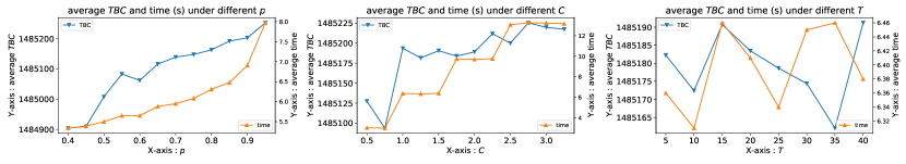
Figure B.1. We study the influence of hyperparameters (i.e., Non-incremental probability $p$, Iteration constant $\mathcal{C}$ and Early stop turn limit $T$) on Confilict dataset with $\beta=1/4$: For each hyperparameter, we execute the algorithm when setting the hyperparameter as various values while keeping other hyperparameters fixed. The results include the average Tolerant Balance Count (TBC) and running time in 25 rounds.

B.3. Stability Study

In our search process (Algorithm 1), we will execute either vertex deletion or color flipping in a certain probability $p$. We conduct some experiments to study how such non-incremental operations help improve the stability of our algorithm, shown in Table B.3.

We modify the algorithm RH to a version with only insertion operations, denoted as RH (insertion only). On all datasets, we execute both algorithms for 100 rounds. As common, we compute the variance $\sigma^{2}$ to measure the stability. Here, for each dataset, we also compute the maximum ($\max\hat{\Phi}$), minimum ($\min\hat{\Phi}$), and average ($\mu$) values for tolerant balance count (TBC).

As shown in Table B.3, we can see with these two operations, the results are more stable and consistent, which can be observed in the rightmost column.

Table B.3. Stability study of Tolerant Balance Count (TBC) under $\beta=1/8$ as example: We conduct 100 rounds of RH and RH (insertion only) on each dataset. The results include maximum TBC ($\max\hat{\Phi}$), minimum TBC ($\min\hat{\Phi}$), mean TBC ($\mu$), and the variance ($\sigma^{2}$) across the 100 rounds. Additionally, we present the variance reduction achieved by considering non-incremental operations.

Dataset	RH (insertion only)				RH				Variance reduction
	$\min\hat{\Phi}$	$\max\hat{\Phi}$	$\mu$	$\sigma^{2}$	$\min\hat{\Phi}$	$\max\hat{\Phi}$	$\mu$	$\sigma^{2}$
Bitcoin	14,864	15,523	15,499	4,977	15,578	15,619	15,604	25	198$\times$
Epinions	462,237	471,120	470,536	1,301,027	472,158	472,240	472,195	315	4,129$\times$
Slashdot	223,054	232,757	232,110	1,564,480	231,988	233,149	232,957	17,521	88$\times$
Twitter	187,549	209,701	208,051	30,265,009	197,072	209,701	209,097	4,455,495	5.7$\times$
Conflict	1,284,391	1,289,332	1,288,405	430,597	1,292,253	1,293,741	1,293,318	84,706	4$\times$
Elections	40,819	42,187	41,981	33,946	42,206	42,358	42,276	1,031	29$\times$
Politics	470,347	470,764	470,576	4,289	470,534	470,905	470,642	4,042	0.06$\times$

Appendix C REPRODUCIBILITY

Codes for our methods and for reproducing all the experimental results are available at GitHub.