Evidence and quantification of memory effects in competitive first passage events

Abstract

Splitting probabilities quantify the likelihood of a given outcome out of competitive events for general random processes. This key observable of random walk theory, historically introduced as the Gambler’s ruin problem for a player in a casino feller68 , has a broad range of applications beyond mathematical finance in evolution genetics, physics and chemistry, such as allele fixation AlfredMoranBook1962 , polymer translocation lua05 , protein folding and more generally competitive reactions espenson95 ; hansen19 ; motti19 . The statistics of competitive events is well understood for memoryless (Markovian) processes VanKampen1992 ; Redner:2001a ; dobramysl2020triangulation ; cheviakov2011optimizing ; bressloff2020target ; bressloff2021first ; condamin2007random ; condamin2006exact ; Condamin2005 ; condamin2008probing ; benichou2014first . However, in complex systems such as polymer fluids, the motion of a particle should typically be described as a process with memory. Appart from scaling theories majumdar10 and perturbative approaches wiese19 in one-dimension, the outcome of competitive events is much less characterized analytically for processes with memory. Here, we introduce an analytical approach that provides the splitting probabilities for general $d$-dimensional non-Markovian Gaussian processes. This analysis shows that splitting probabilities are critically controlled by the out of equilibrium statistics of reactive trajectories, observed after the first passage. This hallmark of non-Markovian dynamics and its quantitative impact on splitting probabilities are directly evidenced in a prototypical experimental reaction scheme in viscoelastic fluids. Altogether, these results reveal both experimentally and theoretically the importance of memory effects on competitive reactions.

Which will you reach first: fortune or ruin? It is ubiquitous that the fate of a system depends on which of a finite set of possible outcomes is realized first, see Fig. 1(a). An historical example is provided by the “gambler’s ruin problem”, in which one wishes to know the risk for a gambler to go bankrupt before making a given profit feller68 . A form of this problem can be traced back to Pascal, and quantifying the risk of ruin has become a classical problem in financial mathematics bouchaud2018trades . In fact, competitive events appear in various domains and under different names; examples include the fixation probability of a mutant in the context of population dynamics AlfredMoranBook1962 , or the nucleation probability in the classical nucleation theory of phase transitions richard18 . In polymer physics, this question emerges in the problems of DNA melting oshanin09 ; lubensky02 , protein and RNA hairpin folding best05 ; chodera11 , polymer translocation through a small pore lua05 and crystallization guttman82 ; mansfield88 , polymer adsorption/desorption kinetics wittmer94 and, related to it, cell adhesion jeppesen01 ; bell17 . Another important field of applications, to which we will refer through this paper, is given by competing (also known as parallel or concurrent) chemical espenson95 , biochemical hansen19 or photochemical motti19 reactions.

The key quantity characterizing generic competitive events is the splitting probability, i.e. the probability, for a random process, of realizing first a given event before several others could occur, and as such belongs to the class of first-passage observables. Most of available theoretical methods to determine splitting probabilities are limited to 1–dimensional Markovian processes VanKampen1992 ; Redner:2001a . Recent advances have considered the extension to higher dimensions for Brownian random walks  dobramysl2020triangulation ; cheviakov2011optimizing ; bressloff2020target ; bressloff2021first ; condamin2007random ; condamin2006exact ; Condamin2005 and general Markovian processes (i.e., processes without memory) condamin2008probing ; benichou2014first .  However, memory effects are essential in complex systems since they emerge as soon as the evolution of the random walker, or of the reaction coordinate, arises from interactions with other (possibly hidden) degrees of freedom. For example, the motion of a monomer in a macromolecule Panja2010 ; bullerjahn2011monomer ; sakaue2013memory , or that of a particle in a crowded narrow channel wei2000single , display strong memory effects. Another well known experimental example of a non-Markovian process (to be studied below) is the motion of a tracer bead in a viscoelastic solution mason1997particle ; mason1995optical ; squires2010fluid ; furst2017microrheology , for which examples of mean square displacement (MSD) functions are shown on Fig. 1(b), which clearly display several temporal regimes and strongly differ from Brownian motion, as expected in such complex fluids vanZanten2004brownian . The Gaussian nature of this process, as seen on Fig. 1(c), together with the temporal non-linearity of the MSD, ensures that the observed process is indeed non-Markovian kallenberg1997foundations .

However, a general theory to quantify the impact of memory effects on splitting probabilities is lacking. Indeed, in the context of first-passage problems for non-Markovian processes, theoretical approaches have mainly been limited to the case of single targets guerin16 ; ReviewBray ; levernier2019survival ; dolgushev15 ; delorme2015maximum ; sadhu2018generalized ; Levernier2022Everlasting ; walter2021first ; levernier2020kinetics . In the case of two targets, the prediction of splitting probabilities is limited to 1–dimensional processes, in a few specific examples masoliver1986first ; bicout2000absorption or for scale invariant processes using scaling arguments majumdar10 or perturbative methods wiese19 .

Here, we introduce a general non-perturbative formalism to predict the outcome of competitive events for the wide class of Gaussian processes. Strikingly, on the basis of a prototypical experimental reaction scheme with tracer beads in viscoelastic fluids, we provide a direct experimental evidence of the impact of memory effects on competitive reactions [see Fig. 1(d) for illustration], in agreement with our theoretical predictions, while so far experimental observations of first passage properties of non-Markovian processes have been limited to persistence exponents ReviewBray ; wong2001measurement or passage over barriers ginot2022barrier ; ferrer2021fluid . In particular, our observations provide a direct experimental proof that the state of the system (constituted by the random walker and the additional degrees of freedom of its environment) at the first passage event is not an equilibrium state. Our theory extends to dimensions higher than 1, providing a path towards the understanding of competitive diffusion limited reactions in complex systems.

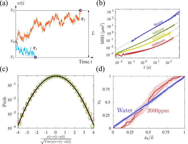
Figure 1: (a) Sketch of the problem of competitive events investigated in this paper: in presence of two targets, for a random walk, what is the probability to hit one target before the other? (b) Experimental Mean Square Displacement (MSD) of tracer particles of $1\mu$m diameter in viscoelastic fluids, with polymer concentrations (from top to bottom) $c=0$ ppm (blue), $c=500$ ppm (green), $c=1000$ ppm (yellow) and $c=2000$ ppm (red). The dashed lines are fits using Eq. (9). (c) normalized histograms of the increments $x(t+\tau)-x(t)$ for $\tau=\tau_{0}$ (crosses) and $\tau=\tau_{0}/2$ (circles) for the three polymer concentrations of $(c)$ (with the same color code). Here $\tau_{0}$ is the memory time of the solution defined in Eq. (9), with $\tau_{0}\simeq 1.48$ s for $c=500$ppm, $\tau_{0}\simeq 2.9$ s for $c=1000$ ppm and $\tau_{0}\simeq 7$ s for $c=2000$ ppm. The black line is the density of a normalized Gaussian, $p(x)=e^{-x^{2}/2}/\sqrt{2\pi}$. (d) Values of the splitting probabilities measured for beads in water (blue curves) and in viscoelastic fluids at $c=2000$ ppm (red) in our experiments and theory (dotted lines), for $x_{0}=0.2\mu$m and $L=0.6\mu$m.

General formalism. We first consider a random walker of position $x(t)$ evolving in continuous time $t$ in a one-dimensional space (the generalization to higher-dimensions will be considered afterwards). We assume that the random walk is symmetric (no privileged direction) and that the increments are stationary (no aging). The initial position is $x_{0}$. We also assume that the process $x(t)$ is continuous (no jumps) and non-smooth (with formally infinite velocity, as in the case of overdamped processes and in particular of Brownian motion), and that it has Gaussian statistics. With these hypotheses, the process is fully characterized by its average ($\langle x(t)\rangle=x_{0}$) and the MSD function $\psi(t)=\langle[x(t)-x_{0}]^{2}\rangle$. Last, we assume that, at long times only, $\psi(t)$ behaves as $\psi(t)\simeq\kappa\ t^{2H}$ with $\kappa>0$ and $0<H<1$. The process is therefore assumed to be diffusive ($H=1/2$), subdiffusive ($H<1/2$) or superdiffusive $(H>1/2)$ at long times, the hypothesis $H>0$ ensures that the particle does not remain trapped around a given position. With these hypotheses one describes a large class of non-Markovian random walks, and in particular diffusion of beads attached to macromolecules Panja2010 ; Panja2010a ; bullerjahn2011monomer ; blumen2004generalized ; Dolgushev2009 , or moving in viscoelastic fluids mason1997particle ; mason1995optical or crowded narrow channels wei2000single , etc.

We now consider two perfectly absorbing targets at positions $x_{1}=0$ and $x_{2}=L$ (with $0<x_{0}<L$). The random walk ends whenever one of these two regions is reached and we aim to calculate $\pi_{i}$, the probability that the target $i\in\{1;2\}$ is reached first. In the single target problem guerin16 ; levernier2019survival ; levernier2020kinetics , it was previously shown that a key quantity to predict first passage statistics is the average trajectory after first contact, if the random walker were allowed to continue its motion. We thus introduce $\mu_{1}(t)$ and $\mu_{2}(t)$, the average trajectories at a time $t$ after a first contact with targets $1$ and $2$, respectively. The following probabilistic argument enables one to understand why $\mu_{1}$ and $\mu_{2}$ are inherently linked to the splitting probabilities. At long times, the average of $x(t)$ (without targets) is clearly $x_{0}$, but on the other hand the average of $x$ can be computed by partitioning over the first contacts with each of the targets, leading to

$$x_{0}=\lim_{t\to\infty}[\pi_{1}\mu_{1}(t)+\pi_{2}\mu_{2}(t)].$$ (1)

Note that, for the (Markovian) Brownian motion, $\mu_{1}=0$ and $\mu_{2}=L$ so that the above argument leads to the well-known result $\pi_{2}=x_{0}/L$. In the more general case of non-Markovian processes, this equations is key to evaluate $\pi_{1}$ (and $\pi_{2}=1-\pi_{1}$), but requires the knowledge of $\mu_{1}$ and $\mu_{2}$. A self-consistent equation for $\mu_{1}$ and $\mu_{2}$ can be obtained by assuming that the statistics of trajectories after a first contact is Gaussian, with the same covariance as that of the original process (see Supplementary Information (SI), Section A). These assumptions are well supported by simulations (Supplementary Figure 1 in SI, Section B). The equations for $\mu_{1},\mu_{2}$ are, for $i\in\{1,2\}$:

$$0 =\sum_{j=1}^{2}\pi_{j}\int_{0}^{\infty}dt\Big{(}p(x_{i},t)(x_{0}-x_{i})[1-K(t,\tau)]$$

$$-q_{j}(x_{i},t)\{\mu_{j}(t+\tau)-x_{i}-[\mu_{j}(t)-x_{i}]K(t,\tau)\}\Big{)},$$ (2)

with

$$K(t,\tau)=[\psi(t+\tau)+\psi(t)-\psi(\tau)]/[2\psi(t)],$$

$$q_{j}(x_{i},t)=\frac{e^{-\frac{(x_{i}-\mu_{j}(t))^{2}}{2\psi(t)}}}{[2\pi\psi(t)]^{1/2}},\ \ p(x_{i},t)=\frac{e^{-\frac{(x_{i}-x_{0})^{2}}{2\psi(t)}}}{[2\pi\psi(t)]^{1/2}}.$$ (3)

The above equations (2) can be solved numerically to evaluate $\mu_{1}(t)$ and $\mu_{2}(t)$, and therefore $\pi_{1}$ and $\pi_{2}$ by using Eq. (1), for arbitrary $\psi(t)$.

Several comments are in order. First, for weakly non-Markovian processes, i.e. when one can write $\psi(t)=2Dt+\varepsilon\psi_{1}(t)$, with $\varepsilon$ a small parameter, our theory provides exact results at order $\varepsilon$ (SI, Section E), and we obtain explicit formulas for the splitting probability at this order for any $\psi_{1}$, which agree with the result of Ref. wiese19 found with other methods in the particular case where $\psi(t)=\kappa\ t^{2H}$ with $H\to 1/2$. Second, we compare the predictions of our formalism to simulation results for several stochastic processes, including strongly non-Markovian processes. To this end we consider two paradigmatic examples of Gaussian non-Markovian processes: (1) the fractional Brownian motion (fBM) with MSD $\psi(t)=\kappa\ t^{2H}$, which is scale invariant (at all times), this model displays long range memory effects and appears in various fields; in particular it can describe the dynamics of a monomer of an infinite polymer chain Panja2010 ; bullerjahn2011monomer ; sakaue2013memory , or of a tagged particle in single file diffusion wei2000single ; (2) the “bi-diffusive” process, with MSD $\psi(t)=t+B(1-e^{-t})$ (in dimensionless variables). This process appears when $x(t)$ is driven by the sum of a white noise and a colored one, with only one relaxation time, as in a Maxwell fluid grimm2011brownian . Numerical simulations of these processes show a quantitative agreement with our theoretical predictions for $\pi_{2}$ in all cases (see Fig. 2). Of note, the Markovian prediction $\pi_{2}=x_{0}/L$ can either strongly underestimate [Fig. 2(a)] or overestimate [Fig. 2(b),(c)] $\pi_{2}$, with an obviously incorrect scaling behavior at small $x_{0}$, while our approach remains quantitative in this regime.

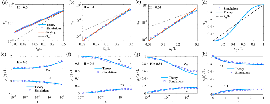
Figure 2: (a) Splitting probability for a superdiffusive fBM with $H=0.6$. Symbols are simulation results obtained with the circulant matrix algorithm Dieker2004 ; dietrich1997fast (statistical error is smaller than symbol sizes). The blue continuous line is the theoretical prediction, obtained by numerically solving Eqs. (1) and (2). The red dashed line is the scaling (4) with the prefactor $A_{H}$ predicted by our theory. The black dashed line is the formula $\pi_{2}=x_{0}/L$, obtained by setting $\mu_{1}=0$ and $\mu_{2}=L$, that overlooks non-Markovian effects. (b),(c) Splitting probability for a sub-diffusive fBMs ($H=0.4$ and $H=0.34$), with the same color code as in (a). (d) Splitting probabilities for a non-scale invariant process with MSD $\psi(t)=t+10(1-e^{-t})$ (bidiffusive process), when the separation between the targets is $L=20$ (in dimensionless units), with the same color code as in (a-c). (e),(f),(g),(h): Average trajectories $\mu_{i}(t)$ in the future of first passage events as measured in simulations (symbols) and predicted by our theory (lines), for $x_{0}/L=0.2$, for the processes corresponding to (a)-(d), respectively. In (e)-(g), the time $t$ is in units of $(L/\sqrt{\kappa})^{1/H}$.

Third, we analytically examine the case of scale invariant processes, $\psi(t)=\kappa\ t^{2H}$, for which the dependence on the geometric parameters $x_{0}$ and $L$ can be extracted. For $x_{0}\ll L$, we find

$$\pi_{2}\simeq A_{H}(x_{0}/L)^{1/H-1},$$ (4)

where the prefactor $A_{H}$ is determined below. Of note, this scaling behavior is consistent with that obtained from scaling arguments in Ref. majumdar10 for 1-dimensional processes, and extended in Ref. levernier2018universal to higher dimensions, in agreement with earlier predictions for Markovian scale invariant processes condamin2008probing . Our approach in addition provides the quantitative determination of the prefactor $A_{H}$, unknown so far. Indeed, when $x_{0}/L\ll 1$, $\mu_{2}$ is not expected to depend on $x_{0}$, whereas $\mu_{1}$ varies at two time scales: the typical time to travel a distance $x_{0}$, equal to $\tau_{1}=(x_{0}/\sqrt{\kappa})^{1/H}$, and the time to travel a distance $L$, equal to $\tau_{2}=(L/\sqrt{\kappa})^{1/H}$. We find that the structure of $\mu_{1}$ in terms of matched asymptotic expansions is

$$\mu_{1}(t,x_{0})\simeq\begin{cases}x_{0}\ \mu_{\infty}(t/\tau_{1})&(t\ll\tau_{2})\\ x_{0}-x_{0}\left(\frac{x_{0}}{L}\right)^{\frac{1}{H}-2}\chi(t/\tau_{2})&(t\gg\tau_{1})\end{cases}$$ (5)

$$\mu_{2}(t,x_{0})\simeq L\ m_{2}(t/\tau_{2})$$ (6)

where $\mu_{\infty},m_{2}$ and $\chi$ are dimensionless scaling functions satisfying equations identified in SI (Section C). Using Eq. (1), it is clear that our formalism yields the scaling (4) and provides the value of the prefactor $A_{H}=(\chi/m_{2})_{t\to\infty}$, in excellent agreement with simulation results (see Fig. 2).

Experiments. We have experimentally measured first passage events for non-Markovian processes by observing the motion of micrometer sized beads in viscoelastic large polymer weight solutions (details on experiments can be found in Methods and SI, Section D). The motion of the beads along one axis $x(t)$ was tracked by using optical microscopy. This type of experimental set-up is standard in microrheology waigh2005microrheology ; mason1997particle ; mason1995optical ; squires2010fluid ; furst2017microrheology but is usually used to measure viscoelastic parameters and not first passage properties. The motion of the beads can be interpreted as obeying an overdamped Generalized Langevin Equation (GLE)

$$\int_{0}^{t}dt^{\prime}K(t-t^{\prime})\dot{x}(t^{\prime})=\xi(t),$$ (7)

where the Gaussian noise $\xi(t)$ has vanishing average and satisfies $\langle\xi(t)\xi(t^{\prime})\rangle=k_{B}TK(|t-t^{\prime}|)$. The measured MSDs in Fig. 1(c) typically display two regimes: one long time diffusive regime and one short time regime where one observes apparent anomalous diffusion. This suggests that, to account for the observed trajectories, one can use a friction kernel of the form of

$$K(t)=\frac{\gamma_{0}\tau_{0}^{\alpha-1}e^{-t/\tau_{0}}}{\Gamma(1-\alpha)t^{\alpha}},$$ (8)

where $\tau_{0}$ is the relaxation time of the polymer solution, $\gamma_{0}=\int_{0}^{\infty}dtK(t)$ is the long-time friction coefficient and $\alpha$ is the subdiffusion exponent at small times. For this memory friction kernel, the MSD reads

$$\psi(t)=\frac{2k_{B}T\tau_{0}}{\gamma_{0}}f(t/\tau_{0}),$$ (9)

$$f(y)=\left[(y-\alpha+1)\gamma(\alpha,y)+y^{\alpha}e^{-y}\right]/\Gamma(\alpha),$$ (10)

where $\gamma(\alpha,y)=\int_{0}^{y}t^{\alpha-1}e^{-t}dt$ is the lower incomplete gamma function. With this choice of kernel, the MSD displays a short time anomalous diffusive regime $\psi(t)\propto t^{\alpha}$ and a long time diffusive one, and $\tau_{0}$ is the crossover time between these regimes. The fits of experimental MSD curves show a good agreement, as seen on Fig. 1(b), and support this choice of function for $K$. We checked that the stochastic process $x(t)$ in the experiment is Gaussian [Fig. 1(c)] and unbiased (SI, Section D), as it should be if it is a realization of the GLE (7), and as implicitly assumed in all microrheology experiments.

Next, we investigated the first passage properties of a trajectory $x(t)$ starting at $x(t_{0})=x_{0}$: we measured the variable $\eta$ defined as $\eta=1$ if a fictitious target at position $L$ is hit before the position $0$. To obtain enough statistics, we considered that $x(t_{0})$ and $x(t_{1})$ could be used as independent starting positions if the time elapsed between $t_{1}$ and $t_{2}$ is larger than $2\tau_{0}$ (or $2$s in water). Then, $\pi_{2}(x_{0},L)$ was calculated as an ensemble average $\langle\eta\rangle$ over different starting positions on each trajectory for various bead trajectories. In our experiments, we made sure that the frame rate is large enough to consider that the typical distances traveled during each time step $dt$ is much smaller than $L$. The results for $\pi_{2}$ are displayed on Fig. 3(b-d). It is clear that for strongly viscoelastic solutions, for which $\alpha$ is the lowest, the curve $\pi_{2}(x_{0})$ is very different from a straight line (which is the result for Markovian diffusion, see Fig. 3(a)), indicating that the probability to hit the closest target is increased by memory effects. This comes from the fact that, in polymer fluids, the motion of a tracer bead induces a delayed response of the surrounding polymer network, tending to bring it back to previously occupied positions, inducing a “denser” exploration of space and a larger probability to hit the closest targets. Furthermore, the experimental values of $\pi_{2}$ are in good agreement with our theoretical predictions, for all parameters.

In our experiments, we also measured the trajectories $\mu_{1}(t),\mu_{2}(t)$ followed by $x(t)$ after the first passage events, which are the hallmarks of non-Markovian effects in the theoretical approach above. These trajectories are displayed on Fig. 3(f-h) where it is clearly seen that, on average, $x(t)$ does not stay at $x=0$ or $x=L$ after the targets have been reached. These trajectories $\mu_{1}$ and $\mu_{2}$ are in quantitative agreement with their predicted values. In our experiments, the motion of a bead with an equilibrium initial condition would be unbiased. In turn, our observation that $\mu_{i}\neq x_{i}$ indicates that the state of the polymer fluid upon a first-passage event at a target is not an equilibrium state. Physically, this comes from the fact that the fluid exerts a delayed response force tending to bring the bead back to its previously occupied positions, which, in our situation, are inside the interval $[0,L]$. This effect is, as expected, not present in solutions without polymers, see Fig. 3(e). Our observations thus constitute a direct experimental proof showing unambiguously that the state of a system (constituted by the bead and the surrounding polymer fluid) upon a first-passage event is not an equilibrium one, which is crucial to understand first passage properties.

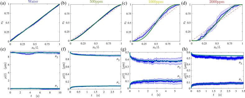
Figure 3: (a-d) Values of the splitting probabilities measured in experiments (blue lines, surrounded by estimates of $95\%$ errorbars), compared with the prediction of our theory (green line). The polymer concentration is indicated on each graph. We also show the result for Markovian diffusion $\pi_{2}=x_{0}/L$ (red dashed line). (e-h) Average trajectories $\mu_{1}$ and $\mu_{2}$ after the first passage to targets $1$ and $2$, as measured in the experiments (blue lines) and predicted by the theory (green lines). Parameters: (a),(e): $c=0$ppm (water) and $L=9\mu$m, (b), (f): $c=500$ ppm and $L=1\mu$m, (c),(g): $c=1000$ ppm and $L=0.5\mu$m, (d),(h): $c=2000$ ppm and $L=0.6\mu$m. In (e), $x_{0}=2\mu$m, in (f-h), $x_{0}=0.2\mu$m.

Extension to higher spatial dimensions ($d>1$). Importantly, our theory can be generalized to higher dimensions, which is relevant to describe general competitive reactions. We denote the $d$–dimensional trajectory of the random walker by $\mathbf{r}(t)=(x_{1}(t),x_{2}(t),...x_{d}(t))$, where all $x_{i}(t)$ satisfy the hypotheses used for the motion of $x(t)$ in 1D. We also assume isotropy, so that the coordinates $x_{i}(t)$ are independent. We further assume the presence of two targets of finite radius $a$ around locations $\mathbf{r}_{1}$ and $\mathbf{r}_{2}$, while $\mathbf{r}_{0}$ is the starting position. Assuming that the dynamics takes place in a large confining domain of volume $V$, we show in SI (Section F) that

$$\pi_{1}=\frac{h_{22}-h_{12}}{h_{22}+h_{11}-h_{21}-h_{12}}=1-\pi_{2},$$ (11)

where

$$h_{ij}=\int_{0}^{\infty}dt\ [q_{j}(\mathbf{r}_{i},t)-p(\mathbf{r}_{i},t)],$$ (12)

where $q_{j}(\mathbf{r},t)$ is the probability density function of the position $\mathbf{r}$ at a time $t$ after the first passage to target $j$, and $p$ is the probability density of the initial process. Note that, in our formalism, the propagators appearing in Eq. (88) are evaluated by considering the dynamics in infinite space (without confining boundaries nor targets). The above equations generalize similar equations for Markovian processes condamin2008probing ; benichou2014first to non-Markovian ones. Although the expressions are similar, the main difference from Markovian processes is that here the propagators have to be evaluated in the future of first passage events, which can strongly differ from the dynamics in the future of a stationary state. In $d=1$, Eq. (86) is an alternative formula to estimate $\pi_{i}$ which however gives results that are indistinguishable from those obtained with Eq. (1), see SI (Section F, Supplementary Fig. 3).

In $d-$dimensions, geometric effects are more difficult to take into account than in the 1D case, since it is necessary to evaluate in which direction the random walker moves after hitting a target. We address this problem by using the following approximations: (i) we work within a decoupling approximation, so that the statistics of paths in the future of the first passage to target $i$ is assumed to be the same as in the single target problem, (ii) we assume that the paths in the future of a first contact with target $i$ at hitting angle $\theta$ follow a Gaussian distribution, with mean $\mu_{i}(t)$ oriented along this angle $\theta$, which it-self has a distribution $\pi(\theta)\propto e^{\alpha\cos\theta}$. We have written self-consistent equations for $\mu_{i}(t)$ and $\alpha$ (see SI, Section F), which provide $\pi_{2}$. The results shown in Fig. 4 demonstrate that our theory captures quantitatively the effects of memory on the kinetics of competitive reactions in dimension higher than one.

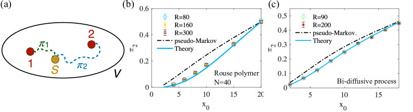
Figure 4: (a) Sketch of the competitive event problem in two dimensions. (b) Splitting probability when the random walker is the first monomer of bead-spring (Rouse) polymer chain of $N=40$ monomers, whose dynamics obeys $\partial_{t}\mathbf{x}_{i}=(\mathbf{x}_{i+1}-2\mathbf{x}_{i}+\mathbf{x}_{i+1})+\mathbf{f}_{i}(t)$, with the prescription $\mathbf{x}_{0}=\mathbf{x}_{1}$ and $\mathbf{x}_{N}=\mathbf{x}_{N+1}$ at the ends, with $\langle f_{i}^{\alpha}(t)f_{j}^{\beta}(t^{\prime})\rangle=2\delta_{\alpha\beta}\delta_{ij}\delta(t-t^{\prime})$, with $i,j$ the monomers’ indexes and $\alpha,\beta$ the spatial coordinates. Symbols are simulation results, the blue line represents the theoretical prediction [Eqs. (86) and (88)] and the black semi-dashed line is the pseudo-Markov approximation, obtained by using $\mu_{i}(t)=0$ in Eqs. (86) and (88). (c) Splitting probability for the bidiffusive process with MSD $\psi(t)=t+10(1-e^{-t})$ for each coordinate. In both cases, the confining volume is a disk of radius $R$ (whose value is given in legend), the first target is at the center and has a radius $a$, and the second target is located at a distance $L=40$ from the center of the first target. $x_{0}$ is the distance to the first target of the initial position, located on the line joining the centers of the targets. In (b), $a=2$ and in (c) $a=1$.

Conclusion. Here we have presented a general theory that predicts the effect of memory on the outcome of competitive events, quantified by the splitting probability to reach one target before the other for Gaussian stochastic processes. Our theory is exact at first non-trivial order for weakly non-Markovian processes and, beyond this perturbative regime, in quantitative agreement with both numerical simulations and experiments where the realization of the random walk is the motion of a tracer bead in a viscoelastic fluid. Interestingly, for this class of processes, the effect of memory is to increase the probability to hit the closest target (with respect to the Markovian prediction). This effect is also clear by looking at the case of Gaussian subdiffusive processes. This effect is strongly different from the case where subdiffusion arises from random jumps with heavy-tailed distributed waiting times, since the distribution of waiting times does not influence splitting probabilities condamin2008probing . Our experiments also unambiguously demonstrate that the state of the system (formed by the bead and the surrounding bath) at the first passage is not an equilibrium one, as seen from the biased dynamics after the first passage events. Our theory can be extended to cover the case of reactions in spatial dimension higher than one, opening a path to the study of the impact of memory effects on competitive reactions in complex media.

METHODS

Preparation of polymer solutions, particles suspension and tracking methods - Polyacrylamide (PAM, molecular weight Mw = 18 $\times$ 10⁶ g/mol, from Polysciences) was dissolved in millipore water (18.2 M$\Omega$cm). 10 mM sodium chloride (NaCl, from Sigma-Aldrich) was added in the solution. The solution was then placed on a digital roller shaker (IKA Roller 6) for around 80 hours at a speed of 20-30 r.p.m. at room temperature to dissolve the polymer completely. The solution was stored in a fridge at 4-6 ^∘C. To minimize the effect of solution ageing, all solutions were used in this study within one month; we checked using rheological measurements that the solutions remained intact for such a period of time. Polystyrene particles from Invitrogen with diameter 1 $\mu$m were used in the experiments. Typically, 1.0 $\mu$L of original particle solution was added into a 2.5-3.0 mL polymer solution. The particles suspension was then mixed by using the digital roller shaker for 10 hours at 20-30 r.p.m. Experiments were carried out under a darkfield inverted microscope (Zeiss AXIO Observer). The diluted particle suspension was sealed inside an adhesive incubation chamber (from Bio-Rad, 9 mm $\times$ 9 mm, 25 $\mu$L). The chamber was covered by a thin cover slide due to the limitation of the working distance of the darkfield condenser. The darkfield condenser was immersed in an optical oil over the microscope, and an objective (Olympus, SLMPLNx100) with magnification 100$\times$ and numerical aperture $0.6$ was used to visualise the particle motion. A motorized translation stage was used to capture microparticles from different areas. All videos were recorded by using a high resolution camera (Hamamatsu, OrcaFlash 4.0 C11440). To minimise the memory effect of the polymer solution, different places were chosen to record the particle motion. All particles were tracked with TrackPy (based on Python). Additional details for the choice of experimental parameters, the estimator of the MSD and its variance, the check of the absence of global drift can be found in SI, Section D.

Supplementary Information

In the supplementary information, we provide

• a detailed derivation of the formalism to calculate the splitting probabilities in $d=1$ (Section A),

• a control of the approximations (Section B),

• an asymptotic analysis of the theory for scale invariant processes (fBM) (Section C),

• details on experimental methods (Section D),

• the proof that the theory is exact at first order for weakly non-Markovian processes and the solution of the perturbation theory (Section E),

• the extension of the formalism to higher dimensions (Section F).

Appendix A Formalism for the two target problem in one dimension

A.1 Derivation of Eq. (1)

In this section, we show that

$$x_{0}=\lim_{t\to\infty}\pi_{1}\mu_{1}(t)+\pi_{2}\mu_{2}(t),$$ (13)

which is Eq. (1) in the main text. We recall that the stochastic process is Gaussian, unbiased, with MSD $\psi(t)$, starting at $x_{0}$, with stationary increments, so that its covariance function is (see e.g. Ref. guerin16 )

$$\text{cov}(x(t),x(t^{\prime}))\equiv\sigma(t,t^{\prime})=\frac{1}{2}\left[-\psi(|t-t^{\prime}|)+\psi(t)+\psi(t^{\prime})\right].$$ (14)

Let us first write the exact relation

$$x_{0}=\int_{0}^{t}dt^{\prime}F(t^{\prime})\mathbb{E}(x(t)|\text{FPT}=t^{\prime})+\mathbb{E}(x(t)|\text{FPT}>t)S(t),$$ (15)

where $F(t)$ is the density of first passage times (to reach either target 1 or target 2), $S(t)=\int_{t}^{\infty}d\tau F(\tau)$ is the survival probability, $\mathbb{E}(x(t)|\text{FPT}=t^{\prime})$ is the average of $x(t)$ given that the first passage time (FPT) is equal to $t^{\prime}$, $\mathbb{E}(x(t)|\text{FPT}>t)$ is the average of $x(t)$ given that the first passage is larger than $t$. We introduce the following “trick”, for any $A>0$ and any function $g(t,t^{\prime})$:

$$\int_{0}^{A}dt\int_{0}^{t}dt^{\prime}\ g(t,t^{\prime})=\int_{0}^{A}dt^{\prime}\int_{t^{\prime}}^{A}dt\ g(t,t^{\prime})=\int_{0}^{A}dt^{\prime}\int_{0}^{A-t^{\prime}}du\ g(t^{\prime}+u,t^{\prime})=\int_{0}^{A}du\int_{0}^{A-u}dt^{\prime}\ g(t^{\prime}+u,t^{\prime}).$$ (16)

Using this property, if we integrate (15) over $t$ between $0$ and $A$, we obtain

$$\int_{0}^{A}dt\ x_{0}=\int_{0}^{A}du\int_{0}^{A-u}dt^{\prime}\ F(t^{\prime})\mathbb{E}(x(t^{\prime}+u)|\text{FPT}=t^{\prime})+\int_{0}^{A}dt\ \mathbb{E}(x(t)|\text{FPT}>t)S(t).$$ (17)

We consider the average trajectory $\mu(t)$ in the future of the FPT:

$$\mu(t)=\langle x(t+\text{FPT})\rangle=\int_{0}^{\infty}dt^{\prime}F(t^{\prime})\mathbb{E}(x(t^{\prime}+t)|\text{FPT}=t^{\prime}).$$ (18)

Using (17) and (18) we obtain

$$\int_{0}^{A}dt\ [\mu(t)-x_{0}]=\int_{0}^{A}du\int_{A-u}^{\infty}dt^{\prime}\ F(t^{\prime})\mathbb{E}(x(t^{\prime}+u)|\text{FPT}=t^{\prime})+\int_{0}^{A}dt\ \mathbb{E}(x(t)|\text{FPT}>t)S(t)\equiv Q(A),$$ (19)

where $Q(A)$ is defined by the above equation. We now wish to show that $Q(A)/A$ vanishes for large $A$. First, we set $v=A-u$:

$$Q(A)=\int_{0}^{A}dv\int_{v}^{\infty}dt^{\prime}\ F(t^{\prime})\mathbb{E}(x(t^{\prime}+A-v)|\text{FPT}=t^{\prime})+\int_{0}^{A}dt\ \mathbb{E}(x(t)|\text{FPT}>t)S(t),$$ (20)

We now argue that, whatever the conditions imposed on the past trajectory, the process at long times cannot travel a distance infinitely larger than the square-root of its mean square displacement $\psi(t)$. Hence, it is natural to assume that, for large $A$

$$|\mathbb{E}(x(t^{\prime}+A-v)|\text{FPT}=t^{\prime})|<K_{1}A^{H},$$ (21)

for some $K_{1}>0$. Furthermore, the absolute value of $x(t)$, given that no boundaries have been reached before $t$, is necessarily less that $L$, so that $|\mathbb{E}(x(t)|\text{FPT}>t)|<L$. Using these arguments, we find

$$|Q(A)|<\int_{0}^{A}dvS(v)(K_{1}A^{H}+L)<(K_{1}A^{H}+L)\int_{0}^{\infty}dvS(v).$$ (22)

Note that $\langle T\rangle=\int_{0}^{\infty}dvS(v)$ is finite in our case, because for times larger than $L^{2}/K$ the random walker is almost sure to have reached one of the two targets. The above expression tells us that $Q(A)$ is at most of order $A^{H}$ for large $A$. Comparing with (19), this means that, for large $t$, $\mu(t)-x_{0}$ is at most of order $1/t^{1-H}$. Hence, for $H<1$, $\mu(t)-x_{0}$ vanishes at large times. Since $\mu=\pi_{1}\mu_{1}+\pi_{2}\mu_{2}$, we obtain the result (13), which is Eq. (1) of the main text.

A.2 Self-consistent equations for $\mu_{1}(t)$ and $\mu_{2}(t)$ [Derivation of Eq. (2)]

Let us consider the equation

$$p(0,t;y,t+\tau)=\int_{0}^{t}dt^{\prime}F(t^{\prime})p(0,t;y,t+\tau|\text{FPT}=t^{\prime}),$$ (23)

which is exact for continuous non-smooth processes. $p(0,t;y,t+\tau)$ is the joint probability density of observing $x(t)=0$ and $x(t+\tau)=y$ (in the absence of any target), with $\tau>0$ and $t>0$. Next, $p(0,t;y,t+\tau|\text{FPT}=t^{\prime})$ is the probability density of observing $x(t)=0$ and $x(t+\tau)=y$ given that the FPT (to reach any of the two targets) is $t^{\prime}$, if the random walker is allowed to continue its motion after the first passage. Using Eq. (16), we obtain

$$\int_{0}^{A}dt\ p(0,t;y,t+\tau)=\int_{0}^{A}du\int_{0}^{A-u}dt^{\prime}F(t^{\prime})p(0,t^{\prime}+u;y,t^{\prime}+u+\tau|\text{FPT}=t^{\prime}).$$ (24)

Now, we introduce the joint probability to observe the position $x$ at time $t$ after the FPT and $y$ at time $t+\tau$ after the FPT:

$$p_{\pi}(x,t;y,t+\tau)=\int_{0}^{\infty}dt^{\prime}\ F(t^{\prime})\ p(x,t^{\prime}+u;y,t^{\prime}+u+\tau|\text{FPT}=t^{\prime}).$$ (25)

Using the trick $\int_{0}^{A-u}(...)=\int_{0}^{\infty}(...)-\int_{A-u}^{\infty}(...)$ and the above definition, Eq. (24) becomes

$$\int_{0}^{A}dt\ [p_{\pi}(0,t;y,t+\tau)-p(0,t;y,t+\tau)]=\int_{0}^{A}du\int_{A-u}^{\infty}dt^{\prime}F(t^{\prime})p(0,t^{\prime}+u;y,t^{\prime}+u+\tau|\text{FPT}=t^{\prime}).$$ (26)

We multiply the above equation by $y$, write $p_{\pi}(0,t;y,t+\tau)=\sum_{j=1}^{2}\pi_{j}q_{j}(0,t;y,t+\tau)$, and integrate over $y$ to obtain

$$\int_{0}^{A}dt\ \left[\sum_{j=1}^{2}\pi_{j}q_{j}(0,t)\mathbb{E}_{\pi_{j}}(x(t+\tau)|x(t)=0)-p(0,t)\mathbb{E}(x(t+\tau)|x(t)=0)\right]=$$

$$\int_{0}^{A}du\int_{A-u}^{\infty}dt^{\prime}F(t^{\prime})p(0,t^{\prime}+u|\text{FPT}=t^{\prime})\mathbb{E}(x(t^{\prime}+u+\tau)|x(t^{\prime}+u)=0;\text{FPT}=t^{\prime})\equiv R(A),$$ (27)

where $R(A)$ is defined by the above equation, $\mathbb{E}_{\pi_{j}}(x(t+\tau)|x(t)=0)$ is the conditional average of $x(t+\tau+\text{FPT})$ given that target $j$ is reached first, and that $x(t+\text{FPT})=0$. We wish now to show that $R(A)\to 0$ for $A\to\infty$. First, setting $u=A-v$ leads to:

$$R(A)=\int_{0}^{A}dv\int_{v}^{\infty}dt^{\prime}F(t^{\prime})p(0,t^{\prime}+A-v|\text{FPT}=t^{\prime})\mathbb{E}(x(t^{\prime}+A-v+\tau)|x(t^{\prime}+A-v)=0;\text{FPT}=t^{\prime}).$$ (28)

For large times, we argue that $p_{\pi}(0,t)\sim K_{0}/t^{H}$ for some $K_{0}>0$, since the distribution of positions extends over a length $t^{H}$. Hence,

$$p(0,t^{\prime}+A-v|\text{FPT}=t^{\prime})\underset{A\to\infty}{\sim}\frac{K_{0}}{A^{H}}.$$ (29)

Next, we argue that there exists a function $h(\tau)$ so that

$$|\mathbb{E}(x(\tau+t^{\prime}+A-v)|x(t^{\prime}+A-v)=0;\text{FPT}=t^{\prime})|<h(\tau),$$ (30)

this is again related to the argument that the particle cannot travel infinitely fast, whatever the conditioning on the past is. With these arguments, we obtain

$$|R(A)|<K_{0}\int_{0}^{A}dv\int_{v}^{\infty}dt^{\prime}F(t^{\prime})\frac{1}{A^{H}}h(\tau)\simeq\frac{1}{A^{H}}\int_{0}^{\infty}dvS(v)h(\tau)\hskip 28.45274pt(A\to\infty).$$ (31)

We conclude that $R(A)$ vanishes for large $A$. Therefore, taking the limit $A\to\infty$ in Eq. (27) leads to

$$\mathcal{H}_{1}(\tau)\equiv\int_{0}^{\infty}dt\ \Bigg{\{} \pi_{1}q_{1}(0,t)\left[\mu_{1}(t+\tau)-\mu_{1}(t)\frac{\sigma(t+\tau,t)}{\sigma(t,t)}\right]+\pi_{2}q_{2}(0,t)\left[\mu_{2}(t+\tau)-\mu_{2}(t)\frac{\sigma(t+\tau,t)}{\sigma(t,t)}\right]$$

$$-p(0,t)\left[x_{0}-x_{0}\frac{\sigma(t+\tau,t)}{\sigma(t,t)}\right]\Bigg{\}}=0,$$ (32)

where we have assumed that the the stochastic process after hitting a target is Gaussian with the stationary covariance approximation, and we have used formulas for conditional averages of Gaussian variables, see e.g. Ref. Eaton1983:

$$\mathbb{E}(X|Y=y)=\mathbb{E}(X)-[\mathbb{E}(Y)-y]\frac{\text{cov}(X,Y)}{\text{var}(Y)}.$$ (33)

Note that, since the process $x(t)$ has stationary increments, the covariance $\sigma(t,t^{\prime})=\text{cov}(x(t),x(t^{\prime}))$ is given by Eq. (14). Finally, with the same reasoning one obtains the equation related to the second target:

$$\mathcal{H}_{2}(\tau)\equiv\int_{0}^{\infty}dt\ \Bigg{\{} \pi_{1}q_{1}(L,t)\left\{\mu_{1}(t+\tau)-[\mu_{1}(t)-L]\frac{\sigma(t+\tau,t)}{\sigma(t,t)}\right\}+\pi_{2}q_{2}(L,t)\left\{\mu_{2}(t+\tau)-[\mu_{2}(t)-L]\frac{\sigma(t+\tau,t)}{\sigma(t,t)}\right\}$$

$$-p(L,t)\left[x_{0}-(x_{0}-L)\frac{\sigma(t+\tau,t)}{\sigma(t,t)}\right]\Bigg{\}}=0.$$ (34)

Eqs. (32) and (34) are equivalent to Eq. (2) of the main text.

Appendix B Validity control of the approximations of the theory

The theory presented in Section relies on two assumptions: (1) the process in the future of the first passage to a target $i\in\{1,2\}$ can be described as a Gaussian process, and (2) the covariance of the future of the first passage is approximated by the covariance of the original process. The validity of these assumptions is checked on Supplementary Figure 5.

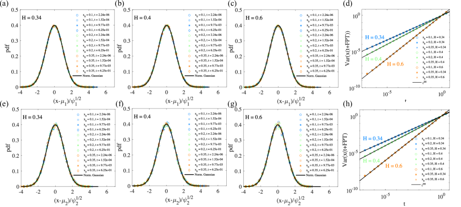
Figure 5: Numerical check of the hypotheses of the theory. (a),(b),(c): normalized histograms of $x(t+\text{FPT})$ given that target $1$ is reached first. The stochastic process has mean square displacement $\psi(t)=t^{2H}$, with (a) $H=0.34$, (b) $H=0.4$, (c) $H=0.6$ and the targets are at $x_{1}=0$ and $x_{2}=L=1$. The time step is $\Delta t=1.5\times 10^{-7}$. Symbols are the results for various values of $t$ and $x_{0}$ indicated in legend. The black line is a normalized Gaussian. (d) variance $\psi_{1}(t)=\text{var}[x(t+\text{FPT})]$ given that target $1$ is reached first. Symbols are simulation results for various $x_{0}$, the black line represents $\psi_{1}(t)=t^{2H}=\psi(t)$. (e),(f),(g),(h): same figures when target $2$ is reached first. Note that for the lowest values of $x_{0}$, the amount of recorded events is less than for target 1, explaining the higher dispersion of the data.

Appendix C Asymptotic behavior of $\pi_{2}$ for scale invariant processes [Derivation of Eq. (4)].

Here, we consider the case $\psi(t)=\kappa\ t^{2H}$ at all times (so that, in the absence of target, $x(t)$ is a fBM). Without loss of generality, we chose the units of length and time so that $L=\kappa=1$. We look for the value of $\pi_{2}$ for small $x_{0}$. We start with the following ansatz for the structure of the solution:

$$\mu_{1}(t,x_{0})\simeq\begin{cases}x_{0}\ \mu_{\infty}(t/x_{0}^{1/H})&t\ll 1,\\ x_{0}-x_{0}^{1/H-1}\ \chi(t)&t\gg x_{0}^{1/H}\end{cases}, \mu_{2}(t,x_{0})\simeq m_{2}(t),$$ (35)

where $\mu_{\infty}$, $\chi$ and $m_{2}$ are scaling functions. This ansatz is justified by the fact that, for small $x_{0}$ it is clear that the time to reach the closest boundary must play a role, so that $\mu_{1}$ must vary at the scale $x_{0}^{1/H}$. It must also vary at the second relevant time scale of the problem, i.e. the time to travel a distance $L$, which in our case is $1$. As shown below, $\mu_{\infty}$ will be the reactive trajectory for the single target problem. Furthermore, the $x_{0}^{1/H-1}$ multiplicative factor of $\chi$ is imposed by the fact that $\mu_{\infty}(t)\simeq 1-B_{\infty}/t^{1-2H}$, so that the small time and large time solutions coincide when $\chi(t)\underset{t\to 0}{\simeq}B_{\infty}/t^{1-2H}$. Finally, it is natural to assume that $\mu_{2}$ does not vary at the scale $x_{0}^{1/H}$. The ansatz (35) will be justified by the fact that one can identify the equations for $\chi$, $m_{2}$ and $\mu_{\infty}$. The equation (13) for $\pi_{1}$ and $\pi_{2}$ leads to

$$1-\pi_{1}=\pi_{2}=A_{H}\ x_{0}^{1/H-1}, A_{H}=\lim_{t\to\infty}\frac{\chi(t)}{m_{2}(t)},$$ (36)

and thus the prefactor $A_{H}$ of the scaling law for the splitting probability can be estimated from the values of $m_{2}$ and $\chi$ at infinity.

The equation for $\mu_{\infty}$ is obtained by estimating $\mathcal{H}_{1}(\tau)$ [defined in Eq. (32)] for $\tau=x_{0}^{1/H}\overline{\tau}$, at fixed $\overline{\tau}$ in the limit of small $x_{0}$, which leads to

$$\int_{0}^{\infty}\frac{dt}{t^{H}}\Bigg{\{}e^{-\mu_{\infty}^{2}(t)/2t^{2H}}\left[\mu_{\infty}(t+\overline{\tau})-\mu_{\infty}(t)\frac{t^{2H}+(t+\overline{\tau})^{2H}-\overline{\tau}^{2H}}{2t^{2H}}\right]-e^{-1/2t^{2H}}\left[1-\frac{t^{2H}+(t+\overline{\tau})^{2H}-\overline{\tau}^{2H}}{2t^{2H}}\right]\Bigg{\}}=0,$$ (37)

which is the equation for the single target problem guerin16 (as expected). Let us identify the equation for $\chi$. With the above scaling ansatz, we estimate that $\mathcal{H}_{1}(\tau)$ reads in the small $x_{0}$ limit (at fixed $\tau$):

$$\mathcal{H}_{1}(\tau)\simeq-x_{0}^{1/H-1}\int_{0}^{\infty}\frac{dt}{t^{H}}\Bigg{\{} \left[\chi(t+\tau)-\chi(t)K(t,\tau)\right]-A_{H}e^{-m_{2}^{2}(t)/(2t^{2H})}\left[m_{2}(t+\tau)-m_{2}(t)K(t,\tau)\right]\Bigg{\}}=0,$$ (38)

this provides an equation for $\chi$ and $m_{2}$. Next, we note that

$$e^{-\frac{[1-\mu_{1}(t)]^{2}}{2\psi}}\simeq e^{-\frac{\left[1-x_{0}+x_{0}^{1/H-1}\chi(t)\right]^{2}}{2t^{2H}}}\simeq e^{-1/(2t^{2H})}\left(1+\frac{x_{0}}{t^{2H}}-\chi(t)\frac{x_{0}^{1/H-1}}{t^{2H}}+...\right), (x_{0}\to 0).$$ (39)

Hence, collecting the terms of order $x_{0}^{1/H-1}$ in $\mathcal{H}_{2}(\tau)$ [defined in Eq. (34)], we obtain

$$\mathcal{H}_{2}(\tau)\simeq x_{0}^{1/H-1}\int_{0}^{\infty}\frac{dt}{t^{H}}\Bigg{\{} \left[-\chi(t+\tau)+\chi(t)K(t,\tau)\right]e^{-1/(2t^{2H})}-\left(A_{H}+\chi(t)\frac{x_{0}^{1/H-1}}{t^{2H}}\right)[-1+K(t,\tau)]e^{-1/(2t^{2H})}$$

$$+A_{H}e^{-[1-m_{2}(t)]^{2}/(2t^{2H})}\left[m_{2}(t+\tau)-1-[m_{2}(t)-1]K(t,\tau)\right]\Bigg{\}}=0,$$ (40)

and thus we have a system of two equations for $\chi$ and $m_{2}$ which we can solve, with the advantage that there are no parameters left (appart from $H$). We also note that we have to look for solutions with $B_{\infty}$ as input, obtained by solving the equation for $\mu_{\infty}$, as in Ref. guerin16 . Some results for $A_{H}$ obtained by numerically solving Eqs. (36), (38) and (40) are reported in table 1.

$H$	$B_{\infty}$	$A_{H}$
0.4	0.75	1.70
0.34	0.49	2.57
0.6	1.05	0.68

Table 1: Values of $B_{\infty}$ (calculated in Ref. guerin16 ) and $A_{H}$, obtained numerically by solving (38) and (40).

Appendix D Details on experimental analysis

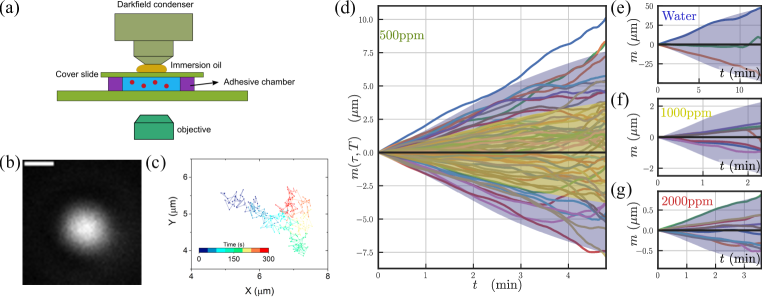
Figure 6: (a) Schematic of darkfield experiment setup. The darkfield condenser is immersed in the optical oil. The thickness of the sample is about 30 $\mu$m sealed inside a slide incubation chamber (from Bio-Rad). (b) Example of image of a particle diffusing in the polymer solution, captured using dark field microscopy. (c) Example of trajectory of a particle diffusing in 2000 ppm polymer solution. The movie was recorded at 250 frame per second (fps) using an objective magnification 100$\times$. Movie duration is about 5min. For clarity, a 1fps trajectory is plotted on the figure. (d)-(e)-(f)-(g) Check of the no-drift hypothesis: we represent the time averaged drift $m(t,\tau)$ defined in Eq. (43). The purple conical regions are $\pm 2\sqrt{\text{var}(m(t,\tau))}$, which should contain $95\%$ of the observations $m(t,\tau)$ in the absence of any drift. In (d) the yellow conical region is $\sqrt{\text{var}(m(t,\tau))}$

Estimation of the MSD and check of the no-drift hypothesis

To estimate the MSD $\psi(t)$ of the tracer particle, we used the following estimator, known as the time-averaged MSD, and defined as

$$\delta^{2}(\tau,T)=\frac{1}{T-\tau}\int_{0}^{T-\tau}dt\ [x(t+\tau)-x(t)]^{2},$$ (41)

where one assumes that a trajectory is observed during a time $T$. Obviously, $\langle\delta^{2}(\tau,T)\rangle=\psi(\tau)$, and the variance of $\delta^{2}$ can be calculated by assuming that $x(t)$ is a Gaussian process (which is suggested by the experimentally observed histograms) with stationary increments. In this case,

$$\text{Var}(\delta^{2}(\tau,T)) =\int_{0}^{T-\tau}dz\frac{T-\tau-z}{(T-\tau)^{2}}\Big{[}\psi(z+\tau)+\psi(|z-\tau|)-2\psi(z)\Big{]}^{2}.$$ (42)

This formula enables us to estimate the precision on the measurement of $\psi$ to $\pm 2\sqrt{\text{Var}(\delta^{2})/N_{\text{traj}}}$, with $N_{\text{traj}}$ the number of independent observed trajectories. We then fit the functional form of the MSD using the equations (9) and (10) in the main text. The fitting parameters are indicated in table 2.

$c$ (ppm)	$\alpha/2$	$\gamma_{0}/k_{B}T$ (s/$\mu$m2)	$\tau_{0}$ (s)
0 (water)	-	2.70	-
500	0.375	40	1.48
1000	0.275	218	2.9
2000	0.175	2.42$\times 10^{3}$	7

Table 2: Parameters of the MSD for the different polymer solutions

To determine if the deviations of $x(t)$ with respect to $x_{0}$ in each trajectory are related to a background drift flow, we estimated the time-averaged increments:

$$m(\tau,T)=\frac{1}{T-\tau}\int_{0}^{T-\tau}dt\ [x(t+\tau)-x(t)].$$ (43)

Under the hypothesis that $x$ satisfies the GLE equation with no drift, $\langle m(\tau,T)\rangle=0$ and its variance is

$$\langle m^{2}(t,\tau)\rangle=\int_{0}^{T-\tau}dz\frac{T-\tau-z}{(T-\tau)^{2}}\Big{[}\psi(z+\tau)+\psi(|z-\tau|)-2\psi(z)\Big{]}.$$ (44)

In all our experiments, about $95\%$ of the observed values of $m(\tau)$ remained in the range $\pm 2\langle m^{2}\rangle^{1/2}$ [calculated with the above formula, see Supplementary Fig. 6(d)-(f)], suggesting that there is no need to assume the existence of a drift to explain the data.

Choice of parameters

The choice of the parameters of the experiments is made to ensure that two conditions are satisfied. First, the displacement $\Delta x$ between two frames has to be small compared to $L$, so that a first passage event between two frames is not missed in the analysis. Since $\Delta x\simeq\sqrt{\kappa_{0}}(\Delta t)^{\alpha/2}$ for small times, where $\kappa_{0}=2\tau_{0}^{1-\alpha}k_{B}T/(\gamma_{0}\Gamma(1+\alpha))$ is the transport coefficient at small times, this condition writes

$$\frac{L}{\Delta x}=\frac{L}{\sqrt{\kappa_{0}}(\Delta t)^{\alpha/2}}\gg 1.$$ (45)

We chose $L$ to be the largest possible that remains in the range where the MSD is not linear, hence at the cross-over between the subdiffusive and the diffusive regime. Next, the memory of the camera limits the number of images that one can acquire during one experiment. For example, at our spatial resolution, the camera can take movies of about 64,000 images. Taking $10$ movies (which represents $640$GB of data), one can record about $n_{0}\simeq 640,000$ images. If we consider that one can use initial conditions separated by $2\tau_{0}$ as independent initial conditions, we estimate the number of first passage events potentially observable as

$$N_{\text{events}}\simeq\frac{(\Delta t)\times n_{0}}{2\tau_{0}}\gg 1$$ (46)

The temporal resolution $\Delta t$ has to be chosen so that both conditions (45) and (46) are satisfied at the same time. For example, for a polymer solution concentrated at $1000$ ppm, with $L=0.5\mu m$, with a frame rate of $245$ frames per seconds, we obtain $L/\Delta x\simeq 7$ and $N_{\text{events}}\simeq 400$, which is the order of magnitudes of the number of events available for $640$ GB of data. In our analysis we could actually observe about $500$ first passage events without the bead leaving the frame or getting close to cell surfaces. Hence, a large amount of data was used to get enough statistics and observe with enough precision non-Markovian effects in the splitting probabilities.

Appendix E First order perturbation theory around Brownian motion ($d=1$)

Here, we show that our theory is exact at first order for weakly non-Markovian processes. Our strategy consists in identifying an exact equation defining the distribution of paths after the first passage, and then checking that, with our Gaussian approximation and the stationary covariance hypothesis, this general equation is satisfied at first order. Next, we give the explicit solution for $\pi_{2}$ at this order, and compare with results of the literature.

E.1 Exactness of the theory at first order

Let us consider a set of times $\tau_{1},...,\tau_{n}$ and a set of positions $\{y_{1},....,y_{N}\}$. We may write the following equation for the probability density of observing the positions $y_{i}$ at times $t+\tau_{i}$:

$$p(x_{i},t;y_{1},t+\tau_{1};...;y_{N},t+\tau_{N})=\int_{0}^{t}\mathrm{d}\tau^{\prime}[ F_{1}(\tau^{\prime})p(x_{i},t;y_{1},t+\tau_{1};...;y_{N},t+\tau_{N}|1,\tau^{\prime})$$

$$+F_{2}(\tau^{\prime})p(x_{i},t;y_{1},t+\tau_{1};...;y_{N},t+\tau_{N}|2,\tau^{\prime})],$$ (47)

where $p(x_{i},t;y_{1},t+\tau_{1};...;y_{N},t+\tau_{N}|j,\tau^{\prime})$ is the probability density of observing $x_{i}$ at $t$ and $y_{k}$ at all $t+\tau_{k}$, given that target $j$ was reached first at $\tau$. Using exactly the same arguments as in Section A.2, this equation leads to

$$\sum_{j=1}^{2}\pi_{j}\int_{0}^{\infty}\mathrm{d}t\,[q_{j}(y_{1},t+\tau_{1};...,y_{N},t+\tau_{N}|x_{i},t)q_{j}(x_{i},t)-p(y_{1},t+\tau_{1};...,y_{N},t+\tau_{N}|;x_{i},t)p(x_{i},t)]=0.$$ (48)

Note that for $N=0$ we obtain:

$$\sum_{j=1}^{2}\pi_{j}\int_{0}^{\infty}\mathrm{d}t\,[q_{j}(x_{i},t)-p(x_{i},t)]=0.$$ (49)

Formally Eq. (48) can be interpreted, in the continuous limit with $N\to\infty$ as

$$\sum_{j=1}^{2}\pi_{j}\int_{0}^{\infty}\mathrm{d}t\,[q_{j}([y(\tau)],t|x_{i},t)q_{j}(x_{i},t)-p([y(\tau)],t|x_{i},t)p(x_{i},t)]=0,$$ (50)

for all continuous paths $[y_{i}(\tau)]$, satisfying $y_{i}(0)=x_{i}$, where $p([y_{i}(\tau)];t|x_{0})$ is the joint probability density to follow this path after the time $t$, i.e. the probability that $x(t+\tau)=y_{i}(\tau)$ for all $\tau$. Similarly, $q_{j}([y_{i}(\tau)],t|x_{i},t)$ is the joint probability density that $x(t+\text{FPT}+\tau)=y(\tau)$, for all $\tau>0$, given that target $j$ was reached first, and that $x(t)=x_{i}$. Note that the condition $x(t)=x_{i}$ can be replaced by the condition that $y(0)=x_{i}$, and using (49) one can write

$$\mathcal{G}_{i}([y])\equiv\sum_{j=1}^{2}\pi_{j}\int_{0}^{\infty}\mathrm{d}t\,\{ [q_{j}([y(\tau)],t|y(0)=x_{i})-p_{s}([y(\tau)]|y(0)=x_{i})]q_{j}(x_{i},t)$$

$$-p(([y(\tau)],t|y(0)=x_{i})-p_{s}([y(\tau)]|y(0)=x_{i})]p(x_{i},t)\}=0,$$ (51)

where the functional $\mathcal{G}_{i}([y])$ is defined by the above equation for all paths $y(\tau)$, and $p_{s}([y(\tau)]|y(0)=x_{i})=\lim_{t\to\infty}p([y(\tau)],t|y(0)=x_{i})$ is the stationary probability to follow a the path $[y]$ given that it starts at $x_{i}$. The process corresponding to $p_{s}$ is a Gaussian process of mean $x_{i}$ and covariance $\sigma(t,t^{\prime})$. The equation $\mathcal{G}_{i}([y])=0$, together with Eq. (49) may thus be seen as a system of equation defining the distribution of paths after the first passage to one of the targets, and the splitting probabilities. Requiring that $\mathcal{G}_{i}([y])=0$ for all paths $[y(\tau)]$ is equivalent to requiring that the following functional vanishes for all functions $[k(\tau)]$:

$$\mathcal{F}_{i}([k])\equiv\int\mathcal{D}[y]e^{\mathrm{i}\int_{0}^{\infty}\mathrm{d}\tau k(\tau)y(\tau)}\mathcal{G}_{i}([y]).$$ (52)

In the case that the paths after the FPT are Gaussian distributed, with mean $\mu_{j}(\tau)$ and covariance $\gamma_{j}(\tau,\tau^{\prime})$ if target $j$ is reached first, we can evaluate this functional:

$$\mathcal{F}_{i}([k])=\int_{0}^{\infty}\mathrm{d}t\sum_{j=1}^{2}\pi_{j}$$

$$\Bigg{\{}q_{j}(x_{i},t)\Big{[}e^{\mathrm{i}\int_{0}^{\infty}\mathrm{d}\tau k(\tau)A_{i}^{\pi_{j}}(t,\tau)-\frac{1}{2}\int_{0}^{\infty}\mathrm{d}\tau\int_{0}^{\infty}\mathrm{d}\tau^{\prime}k(\tau)k(\tau^{\prime})B_{i}^{\pi_{j}}(t,\tau,\tau^{\prime})}-e^{\mathrm{i}\int_{0}^{\infty}\mathrm{d}\tau k(\tau)x_{i}-\frac{1}{2}\int_{0}^{\infty}\mathrm{d}\tau\int_{0}^{\infty}\mathrm{d}\tau^{\prime}k(\tau)k(\tau^{\prime})\sigma(\tau,\tau^{\prime})}\Big{]}$$

$$-p(x_{i},t)\Big{[}e^{\mathrm{i}\int_{0}^{\infty}\mathrm{d}\tau k(\tau)A_{i}(t,\tau)-\frac{1}{2}\int_{0}^{\infty}\mathrm{d}\tau\int_{0}^{\infty}\mathrm{d}\tau^{\prime}k(\tau)k(\tau^{\prime})B_{i}(t,\tau,\tau^{\prime})}-e^{\mathrm{i}\int_{0}^{\infty}\mathrm{d}\tau k(\tau)x_{i}-\frac{1}{2}\int_{0}^{\infty}\mathrm{d}\tau\int_{0}^{\infty}\mathrm{d}\tau^{\prime}k(\tau)k(\tau^{\prime})\sigma(\tau,\tau^{\prime})}\Big{]}\Bigg{\}},$$

with

$$A_{i}^{\pi_{j}}(t,\tau)=\mu_{j}(t+\tau)-[\mu_{j}(t)-x_{i}]\frac{\gamma_{j}(t+\tau,t)}{\gamma_{j}(t,t)}, A_{i}(t,\tau)=x_{0}-[x_{0}-x_{i}]\frac{\sigma(t+\tau,t)}{\sigma(t,t)},$$

$$B_{i}^{\pi_{j}}(t,\tau,\tau^{\prime})=\gamma_{j}(t+\tau,t+\tau^{\prime})-\frac{\gamma_{j}(t+\tau,t)\gamma_{j}(t,t+\tau^{\prime})}{\gamma_{j}(t,t)}, B_{i}(t,\tau,\tau^{\prime})=\sigma(t+\tau,t+\tau^{\prime})-\frac{\sigma(t+\tau,t)\sigma(t,t+\tau^{\prime})}{\sigma(t,t)},$$

$$q_{j}(x_{i},t)=\frac{1}{\sqrt{2\pi\gamma_{j}(t,t)}}\exp\left[-\frac{[x_{i}-\mu_{j}(t)]^{2}}{2\gamma_{j}(t,t)}\right], p(x_{i},t)=\frac{1}{\sqrt{2\pi\sigma(t,t)}}\exp\left[-\frac{[x_{i}-x_{0}]^{2}}{2\sigma(t,t)}\right].$$

In the following we consider a small deviation around the Brownian motion, by taking the mean-square displacement $\psi(t)=Kt+\epsilon\psi_{1}(t)+\mathcal{O}(\epsilon^{2})$. We may thus assume that $\mu_{1}$ is close to $x_{1}=0$ and $\mu_{2}$ is close to $x_{2}=L$, leading to the ansatz:

$$\mu_{i}(t)=x_{i}+\epsilon g_{i}(t)+\mathcal{O}(\epsilon^{2}),$$ (53)

$$\gamma_{i}(t,t^{\prime})=\sigma^{(0)}(t,t^{\prime})+\epsilon\gamma_{i}^{(1)}(t,t^{\prime})+\mathcal{O}(\epsilon^{2}), \sigma(t,t^{\prime})=\sigma^{(0)}(t,t^{\prime})+\epsilon\sigma^{(1)}(t,t^{\prime})+\mathcal{O}(\epsilon^{2}),$$ (54)

$$\pi_{2}=(x_{0}+\epsilon p)/L+\mathcal{O}(\epsilon^{2}), \pi_{1}=1-\pi_{2}=(L-x_{0}-\epsilon p)/L+\mathcal{O}(\epsilon^{2}).$$ (55)

Moreover, $\sigma^{(0)}(t,t^{\prime})$ is the covariance of the Brownian motion,

$$\sigma^{(0)}(t,t^{\prime})=\kappa\min(t,t^{\prime}).$$ (56)

At order $\varepsilon^{0}$, we find that $\mathcal{F}_{i}$ vanishes (as expected). At order one, introducing

$$C_{i}=e^{\text{i}\int_{0}^{\infty}d\tau k(\tau)x_{i}-\frac{1}{2}\int_{0}^{\infty}\mathrm{d}\tau\int_{0}^{\infty}\mathrm{d}\tau^{\prime}k(\tau)k(\tau^{\prime})\sigma^{(0)}(\tau,\tau^{\prime})},$$ (57)

the functional $\mathcal{F}_{i}([k])$ can be recast as $\mathcal{F}_{i}([k])=\epsilon\,i\mathcal{F}_{i}^{(1)}([k])+\mathcal{O}(\epsilon^{2}),$ where

$$\mathcal{F}_{i}^{(1)}([k])=\int_{0}^{\infty}\mathrm{d}\tau k(\tau)\left[\left(1-\frac{x_{0}}{L}\right)Q_{i1}(\tau)+\frac{x_{0}}{L}Q_{i2}(\tau)\right]+\int_{0}^{\infty}\mathrm{d}\tau\int_{0}^{\infty}\mathrm{d}\tau^{\prime}k(\tau)k(\tau^{\prime})\left[\left(1-\frac{x_{0}}{L}\right)R_{i1}(\tau,\tau^{\prime})+\frac{x_{0}}{L}R_{i2}(\tau,\tau^{\prime})\right],$$

with

$$Q_{ij}(\tau)=\int_{0}^{\infty}\frac{\mathrm{i}\,\mathrm{d}t}{\sqrt{2\pi\kappa t}}\left\{\left[g_{j}(t+\tau)-g_{j}(t)-(x_{j}-x_{i})\frac{\gamma_{j}^{(1)}(t+\tau,t)-\gamma_{j}^{(1)}(t,t)}{\sigma^{(0)}(t,t)}\right]e^{-\frac{(x_{i}-x_{j})^{2}}{2\kappa t}}-(x_{0}-x_{i})\Delta(t,\tau)e^{-\frac{(x_{0}-x_{i})^{2}}{2\kappa t}}\right\},$$ (58)

where

$$\Delta(t,\tau)=[\sigma^{(1)}(t,t)-\sigma^{(1)}(t+\tau,t)]/\sigma^{(0)}(t,t),$$ (59)

and the value of $R_{ij}$ is:

$$R_{ij}(\tau,\tau^{\prime})= -\int_{0}^{\infty}\frac{\mathrm{d}t}{\sqrt{8\pi\kappa t}}\Big{\{}\left[\gamma_{j}^{(1)}(t+\tau,t+\tau^{\prime})-\gamma_{j}^{(1)}(t+\tau,t)-\gamma_{j}^{(1)}(t,t+\tau^{\prime})+\gamma_{j}^{(1)}(t,t)-\sigma^{(1)}(\tau,\tau^{\prime})\right]e^{-\frac{(x_{i}-x_{j})^{2}}{2\kappa t}}$$

$$-\left[\sigma^{(1)}(t+\tau,t+\tau^{\prime})-\sigma^{(1)}(t+\tau,t)-\sigma^{(1)}(t,t+\tau^{\prime})+\sigma^{(1)}(t,t)-\sigma^{(1)}(\tau,\tau^{\prime})\right]e^{-\frac{(x_{i}-x_{0})^{2}}{2\kappa t}}\Big{\}}.$$ (60)

Now, we show that we can find the functions $\gamma_{j}^{(1)}$ and $g_{j}$ so that $\mathcal{F}_{i}([k])$ vanishes for all $[k(\tau)]$ at order $\varepsilon$, meaning that our theory will be exact at order $\varepsilon$. First, we note that, since $x(t)$ has stationary increments, $\sigma$ satisfies the relation (14) and therefore

$$\sigma(t+\tau,t+\tau^{\prime})-\sigma(t+\tau,t)-\sigma(t,t+\tau^{\prime})+\sigma(t,t)=\sigma(\tau,\tau^{\prime}),$$ (61)

and this is true at all orders of $\varepsilon$. Hence, if one choses $\gamma_{j}^{(1)}(t,t^{\prime})=\sigma^{(1)}(t,t^{\prime})$, then one sees that all $R_{ij}=0$ in Eq. (60). As a consequence, all terms that are quadratic in $k(\tau)$ in the definition of $\mathcal{F}_{i}^{(1)}$ vanish with this choice of $\gamma_{j}^{(1)}(t,t^{\prime})$, meaning that the stationary covariance approximation is exact at first order. Now, for convenience let us write $g_{1}=-f$ and $g_{2}=g$. The terms of $\mathcal{F}_{i}^{(1)}$ that are linear in $k$ vanish if $f$ and $g$ satisfy the integral equations

$$\int_{0}^{\infty}\frac{\mathrm{d}t}{\sqrt{t}}\left\{\frac{L-x_{0}}{L}[-f(t+\tau)+f(t)]+\frac{x_{0}}{L}e^{-\frac{L^{2}}{2Kt}}[g(t+\tau)-g(t)+L\Delta(t,\tau)]-x_{0}e^{-\frac{x_{0}^{2}}{2Kt}}\Delta(t,\tau)\right\}=0,$$ (62)

$$\int_{0}^{\infty}\frac{\mathrm{d}t}{\sqrt{t}}\left\{\frac{L-x_{0}}{L}e^{-\frac{L^{2}}{2Kt}}[-f(t+\tau)+f(t)-L\Delta(t,\tau)]+\frac{x_{0}}{L}[g(t+\tau)-g(t)]-(x_{0}-L)e^{-\frac{(L-x_{0})^{2}}{2Kt}}\Delta(t,\tau)\right\}=0.$$ (63)

In the following we will obtain the functions $f(t)$ and $g(t)$ that satisfy Eqs. (62)-(63). Thus, $\mathcal{F}_{i}^{(1)}$ vanishes for all $[k]$, and we conclude that our hypothesis of Gaussianity of trajectories after the first passage, with the stationary covariance approximation, is exact at least at order $\mathcal{O}(\epsilon^{1})$.

E.2 Explicit solution of the theory at first order

Taking derivative from Eqs. (62)-(63) with respect to $\tau$ gives

$$\int_{0}^{\infty}\mathrm{d}t\left[\frac{L-x_{0}}{L}K_{1}(t)f^{\prime}(t+\tau)-\frac{x_{0}}{L}K_{2}(t)g^{\prime}(t+\tau)\right]=x_{0}I_{1}(\tau),$$

$$\int_{0}^{\infty}\mathrm{d}t\left[\frac{L-x_{0}}{L}K_{2}(t)f^{\prime}(t+\tau)-\frac{x_{0}}{L}K_{1}(t)g^{\prime}(t+\tau)\right]=(x_{0}-L)I_{2}(\tau),$$ (64)

with

$$K_{1}(t)=\frac{1}{\sqrt{t}},\hskip 28.45274ptK_{2}(t)=\frac{e^{-\frac{L^{2}}{2\kappa t}}}{\sqrt{t}},\hskip 28.45274ptI_{i}(t)=\int_{0}^{\infty}\frac{\mathrm{d}t}{\sqrt{t}}\left[e^{-\frac{L^{2}}{2\kappa t}}-e^{-\frac{(x_{i}-x_{0})^{2}}{2\kappa t}}\right]\partial_{\tau}\Delta(t,\tau).$$ (65)

In order to solve the system (64), we consider the auxiliary problem:

$$\int_{0}^{\infty}\mathrm{d}t\left[\frac{L-x_{0}}{L}K_{1}(t)f_{1}^{\prime}(t+\tau)-\frac{x_{0}}{L}K_{2}(t)g_{1}^{\prime}(t+\tau)\right]=x_{0}A_{1}e^{\mathrm{i}\omega\tau},$$

$$\int_{0}^{\infty}\mathrm{d}t\left[\frac{L-x_{0}}{L}K_{2}(t)f_{1}^{\prime}(t+\tau)-\frac{x_{0}}{L}K_{1}(t)g_{1}^{\prime}(t+\tau)\right]=(x_{0}-L)A_{2}e^{\mathrm{i}\omega\tau},$$ (66)

which admits the following obvious solution:

$$f_{1}^{\prime}(t)=\frac{e^{\mathrm{i}\omega t}\ L}{L-x_{0}}\frac{x_{0}A_{1}\tilde{K}_{1}(-\mathrm{i}\omega)+(L-x_{0})A_{2}\tilde{K}_{2}(-\mathrm{i}\omega)}{\tilde{K}^{2}_{1}(-\mathrm{i}\omega)-\tilde{K}^{2}_{2}(-\mathrm{i}\omega)}, g_{1}^{\prime}(t)=e^{\mathrm{i}\omega t}\frac{L}{x_{0}}\frac{x_{0}A_{1}\tilde{K}_{2}(-\mathrm{i}\omega)+(L-x_{0})A_{2}\tilde{K}_{1}(-\mathrm{i}\omega)}{\tilde{K}^{2}_{1}(-\mathrm{i}\omega)-\tilde{K}^{2}_{2}(-\mathrm{i}\omega)},$$ (67)

where $\tilde{h}(s)=\int_{0}^{\infty}dth(s)e^{-st}$ represents the Laplace transform of a function $h$, and thus $\tilde{K}_{i}(-\mathrm{i}\omega)=\int_{0}^{\infty}\mathrm{d}te^{\mathrm{i}\omega t}K_{i}(t)$. The solution of (64) is found by superposition; writing the functions $I_{i}$ as a superposition of exponentials as $I_{j}(\tau)=\int_{-\infty}^{\infty}\frac{\mathrm{d}\omega}{2\pi}\hat{I}_{j}(\omega)e^{\mathrm{i}\omega\tau}$, we obtain

$$f^{\prime}(t)=\frac{L}{L-x_{0}}\int_{-\infty}^{\infty}\frac{\mathrm{d}\omega}{2\pi}\frac{x_{0}\hat{I}_{1}(\omega)\tilde{K}_{1}(-\mathrm{i}\omega)+(L-x_{0})\hat{I}_{2}(\omega)\tilde{K}_{2}(-\mathrm{i}\omega)}{\tilde{K}^{2}_{1}(-\mathrm{i}\omega)-\tilde{K}^{2}_{2}(-\mathrm{i}\omega)}e^{\mathrm{i}\omega t},$$

$$g^{\prime}(t)=\frac{L}{x_{0}}\int_{-\infty}^{\infty}\frac{\mathrm{d}\omega}{2\pi}\frac{x_{0}\hat{I}_{1}(\omega)\tilde{K}_{2}(-\mathrm{i}\omega)+(L-x_{0})\hat{I}_{2}(\omega)\tilde{K}_{1}(-\mathrm{i}\omega)}{\tilde{K}^{2}_{1}(-\mathrm{i}\omega)-\tilde{K}^{2}_{2}(-\mathrm{i}\omega)}e^{\mathrm{i}\omega t}.$$ (68)

Integrating these equation over $t$ and using $f(0)=g(0)=0$ leads to

$$f(t)=\frac{x_{0}L}{L-x_{0}}\Phi_{11}(t)+L\Phi_{22}(t), g(t)=L\Phi_{21}(t)+\frac{(L-x_{0})L}{x_{0}}\Phi_{12}(t),$$ (69)

where

$$\Phi_{ij}(t)=\int_{-\infty}^{\infty}\frac{\mathrm{d}\omega}{2\pi}\frac{e^{\mathrm{i}\omega t}-1}{\mathrm{i}\omega}\frac{\tilde{K}_{i}(-\mathrm{i}\omega)\hat{I}_{j}(\omega)}{\tilde{K}^{2}_{1}(-\mathrm{i}\omega)-\tilde{K}^{2}_{2}(-\mathrm{i}\omega)}=\int_{-\infty}^{\infty}\frac{\mathrm{d}\omega}{2\pi}\frac{e^{\mathrm{i}\omega t}-1}{\mathrm{i}\omega}\frac{\tilde{K}_{i}(-\mathrm{i}\omega)}{\tilde{K}^{2}_{1}(-\mathrm{i}\omega)-\tilde{K}^{2}_{2}(-\mathrm{i}\omega)}\int_{0}^{\infty}\mathrm{d}x\ e^{-\mathrm{i}\omega x}I_{j}(x),$$ (70)

where the last equality follows from the definition of $\hat{I}_{j}(\omega)$ as the Fourier transform of $I_{j}(t)$ (which we consider as vanishing for negative $t$). Now, let us define two functions $W_{1}(t)$ and $W_{2}(t)$ so that their Laplace transforms read:

$$\tilde{W}_{i}(s)=\frac{\tilde{K}_{i}(s)}{s[\tilde{K}_{1}^{2}(s)-\tilde{K}_{2}^{2}(s)]}.$$ (71)

Changing the variables $\omega\to-\omega$ in Eq. (70) leads to

$$\Phi_{ij}(t)=-\int_{0}^{\infty}\mathrm{d}x\int_{-\infty}^{\infty}\frac{\mathrm{d}\omega}{2\pi}\frac{e^{-\mathrm{i}\omega t}-1}{\mathrm{i}\omega}\tilde{W}_{i}(\text{i}\omega)e^{\mathrm{i}\omega x}I_{j}(x)=\int_{0}^{\infty}\mathrm{d}x[-W_{i}(x-t)\theta(x-t)+W_{i}(x)\theta(x)]I_{j}(x),$$ (72)

where in the second equality we have recognized the inverse Laplace transform. Finally, making shift of the variable $x$ in the first term of the above expression and using the definition of $I_{j}$, we arrive to

$$\Phi_{ij}(t)=\frac{1}{2\kappa}\int_{0}^{\infty}\mathrm{d}x\ W_{i}(x)\int_{0}^{\infty}\frac{\mathrm{d}y}{y^{3/2}}\left[e^{-\frac{L^{2}}{2\kappa y}}-e^{-\frac{(x_{j}-x_{0})^{2}}{2\kappa y}}\right][\psi_{1}^{\prime}(x+y+t)-\psi_{1}^{\prime}(x+y)-\psi_{1}^{\prime}(x+t)+\psi_{1}^{\prime}(x)],$$ (73)

This expression, combined with Eq. (69), is an explicit solution for the average trajectories $f$ and $g$ if one specifies the value of $W_{i}$. The functions $W_{i}$ can be calculated as follows. First, using (65) and (71) we obtain

$$\tilde{W}_{1}(s)=\frac{1}{\sqrt{\pi s}\left(1-e^{-\sqrt{8sL^{2}/\kappa}}\right)}=\frac{1}{\sqrt{\pi s}}\sum_{n=0}^{\infty}e^{-n\sqrt{8sL^{2}/\kappa}},$$ (74)

$$\tilde{W}_{2}(s)=\frac{e^{-\sqrt{2sL^{2}/\kappa}}}{\sqrt{\pi s}\left(1-e^{-\sqrt{8sL^{2}/\kappa}}\right)}=\frac{1}{\sqrt{\pi s}}\sum_{n=0}^{\infty}e^{-(n+1/2)\sqrt{8sL^{2}/\kappa}},$$ (75)

where we have used geometric series in order to identify the inverse Laplace transforms of $\tilde{W}_{i}(s)$, leading to:

$$W_{1}(t)=\sum_{n=0}^{\infty}\frac{e^{-2L^{2}n^{2}/(Kt)}}{\pi\sqrt{t}}=\frac{\vartheta_{3}\left(0,e^{-\frac{2L^{2}}{Kt}}\right)+1}{2\pi\sqrt{t}}, W_{2}(t)=\sum_{n=0}^{\infty}\frac{e^{-2L^{2}(n+1/2)^{2}/(Kt)}}{\pi\sqrt{t}}=\frac{\vartheta_{2}\left(0,e^{-\frac{2L^{2}}{Kt}}\right)}{2\pi\sqrt{t}}.$$ (76)

Here, $\vartheta_{k}(\cdot,\cdot)$ is the Jacobi theta function of the $k$th kind. Finally, let us determine now the splitting probability $\pi_{2}=x_{0}/L+\epsilon\pi_{2}^{(1)}+\mathcal{O}(\epsilon^{2})$, at order $\epsilon^{1}$ we obtain from Eq. (1) in the main text

$$\pi_{2}^{(1)}L=\lim_{t\to\infty}[\pi_{1}^{(0)}f(t)-\pi_{2}^{(0)}g(t)].$$

Using the above results, we obtain

$$\pi_{2}^{(1)} =\int_{0}^{\infty}\int_{0}^{\infty}\frac{\mathrm{d}x\mathrm{d}y}{\sqrt{y^{3}x}}\frac{1+\vartheta_{4}\left(0,e^{-\frac{L^{2}}{2\kappa x}}\right)}{4\pi\kappa}\left\{\frac{x_{0}}{L}\left[e^{-\frac{L^{2}}{2\kappa y}}-e^{-\frac{x_{0}^{2}}{2\kappa y}}\right]-\left(1-\frac{x_{0}}{L}\right)\left[e^{-\frac{L^{2}}{2\kappa y}}-e^{-\frac{(L-x_{0})^{2}}{2\kappa y}}\right]\right\}[\psi_{1}^{\prime}(x+y)-\psi_{1}^{\prime}(x)],$$ (77)

where we have used the relation $\vartheta_{3}(0,q)-\vartheta_{2}(0,q)=\vartheta_{4}(0,q^{1/4})$.

E.3 Examples

Fractional Brownian motion. This process is characterized by $\psi(t)=\kappa t^{2H}=\kappa t+\epsilon\psi_{1}(t)+\mathcal{O}(\epsilon^{2})$, so that for $H=1/2+\epsilon$ we have $\psi_{1}(t)=2\kappa t\ln t$. We use the notation $u=x_{0}/L$. The splitting probability has the structure

$$\pi_{2}^{(1)}=Q(u)-Q(1-u),\text{ with }Q(u)\equiv\frac{u}{\pi}\int_{0}^{\infty}\frac{\mathrm{d}x}{\sqrt{x}}\sum_{k=0}^{\infty}(-1)^{k}e^{-\frac{k^{2}}{x}}\int_{0}^{\infty}\frac{\mathrm{d}y}{y^{3/2}}\left[e^{-\frac{u^{2}}{y}}-e^{-\frac{1}{y}}\right]\ln\frac{x+y}{x},$$ (78)

where we have used $\vartheta_{4}(0,e^{-\frac{1}{x}})=1+2\sum_{k=1}^{\infty}(-1)^{k}e^{-\frac{k^{2}}{x}}$. $Q(u)$ can be calculated by integrating first over $y$, and then over $x$, and finally summing over $k$, leading to

$$Q(u) =4u(1-\ln u)+(1-2u)\left[12\ln A-\frac{7}{3}\ln 2\right]-2\ln\pi+8\left[\psi^{(-2)}\left(\frac{u+2}{2}\right)-\psi^{(-2)}\left(\frac{u+1}{2}\right)\right],$$ (79)

where $A\approx 1.28243$ is the Glaisher-Kinkelin constant and $\psi^{(-2)}(\xi)=\int_{0}^{\xi}\mathrm{d}z\ln\Gamma(z)$ is the generalized polygamma function. We note that the constant term can be reformulated as $\ln(A^{12}2^{-\frac{7}{3}}\pi^{-2})=8[\psi^{(-2)}(1/2)-\psi^{(-2)}(1)]$, hence $Q(0)=0$. Note that the result (79) were obtained in Ref. wiese19 based on other methods.

Bi-diffusive process. This process is characterized by $\psi(t)=\kappa t+A(1-e^{-t/\tau})=\kappa t+\epsilon\psi_{1}(t)+\mathcal{O}(\epsilon^{2})$, so that $\psi_{1}(t)=\kappa\tau(1-e^{-t/\tau})$. With this, introducing the dimensionless variables $\ell=L\sqrt{2/(K\tau)}$ and $u=x_{0}/L$, we obtain

$$f(t) =\frac{L[\cosh((1-u)\ell)-(1-u)\cosh(\ell)-u]}{(1-u)\ell\sinh(\ell)}(1-e^{-t/\tau}),\hskip 14.22636ptg(t)=\frac{L[\cosh(u\ell)-u\cosh(\ell)-(1-u)]}{u\ell\sinh(\ell)}(1-e^{-t/\tau}),$$

$$\pi_{2}^{(1)} =\frac{[\cosh((1-u)\ell)-\cosh(u\ell)+(1-2u)(1-\cosh(\ell))]}{\ell\sinh(\ell)}.$$

Appendix F Generalization of the theory to $d\geq 1$

Here we consider the case of spatial dimension $d\geq 1$. In this case we have to specify that the target search problem takes place in a finite confining volume (which is not seen at all if $d=1$ with two targets). The position $\mathbf{r}(t)$ is now a vector $(x_{1}(t),x_{2}(t),...,x_{d}(t))$ and the centers of the targets are located at $\mathbf{r}_{1}$ and $\mathbf{r}_{2}$, these targets have radius $a$ and are inside a large confining volume $V$. We first write the generalized renewal equation:

$$p(\mathbf{r}_{i},t)=\int_{0}^{t}dt^{\prime}F(t^{\prime})p(\mathbf{r}_{i},t|\text{FPT}=t^{\prime}),$$ (80)

where $p(\mathbf{r},t|\Omega)$ represents the probability density of $\mathbf{r}$ at $t$ given the event $\Omega$. Note that $p$ is defined in confined space and tends at large time to a stationary value $p_{s}(\mathbf{r})$ assumed here to be uniform, $p_{s}(\mathbf{r})=1/V$. Substracting $p_{s}$ on both sides of the above equation leads to

$$p(\mathbf{r}_{i},t)-p_{s}(\mathbf{r}_{i})=\int_{0}^{t}dt^{\prime}F(t^{\prime})[p(\mathbf{r}_{i},t|\text{FPT}=t^{\prime})-p_{s}(\mathbf{r}_{i})]-\int_{t}^{\infty}d\tau p_{s}(\mathbf{r}_{i})F(\tau).$$ (81)

Now, the probability density $p_{\pi}$ to observe the position $\mathbf{r}$ at time $t$ after the FPT is defined as

$$p_{\pi}(\mathbf{r},\tau)=\int_{0}^{\infty}dt\ p(\mathbf{r},t+\tau|\text{FPT}=\tau)F(\tau).$$ (82)

We note that, using Eq. (16) with $A=\infty$ and $g(t,t^{\prime})=F(t^{\prime})[p(\mathbf{r}_{i},t|\text{FPT}=t^{\prime})-p_{s}(\mathbf{r}_{i})]$, we obtain

$$\int_{0}^{\infty}dt\int_{0}^{t}dt^{\prime}F(t^{\prime})[p(\mathbf{r}_{i},t|\text{FPT}=t^{\prime})-p_{s}(\mathbf{r}_{i})] =\int_{0}^{\infty}du\int_{0}^{t}dt^{\prime}F(t^{\prime})[p(\mathbf{r}_{i},t^{\prime}+u|\text{FPT}=t^{\prime})-p_{s}(\mathbf{r}_{i})]$$

$$=\int_{0}^{\infty}du\ [p_{\pi}(\mathbf{r}_{i},u)-p_{s}(\mathbf{r}_{i})]$$ (83)

Noting also that $\langle T\rangle=\int_{0}^{\infty}dt\int_{t}^{\infty}F(t^{\prime})dt^{\prime}$, we see that integrating (81) over $t\in]0,\infty[$ leads to the exact relation

$$\langle T\rangle p_{s}(\mathbf{r}_{i})=\int_{0}^{\infty}dt\ [p_{\pi}(\mathbf{r}_{i},t)-p(\mathbf{r}_{i},t)].$$ (84)

Partitioning over first passage to each of the targets leads to

$$p_{\pi}(\mathbf{r},t)=\pi_{1}q_{1}(\mathbf{r},t)+\pi_{2}q_{2}(\mathbf{r},t),$$ (85)

where $q_{j}(\mathbf{r},t)$ is the probability density function (pdf) of $\mathbf{r}$ at a time $t$ after the first passage to target $j$. Hence, Eq. (84) leads to a system of equations for $\pi_{1},\pi_{2},\langle T\rangle$ which is completed by the relation $\pi_{1}+\pi_{2}=1$, so that

$$\pi_{1}=\frac{h_{22}-h_{12}}{h_{22}+h_{11}-h_{21}-h_{12}}=1-\pi_{2}$$ (86)

$$\frac{\langle T\rangle}{V}=\frac{h_{11}h_{22}-h_{12}h_{21}}{h_{22}+h_{11}-h_{21}-h_{12}}.$$ (87)

where

$$h_{ij}=\int_{0}^{\infty}dt[q_{j}(\mathbf{r}_{i},t)-p(\mathbf{r}_{i},t)],$$ (88)

We stress that the above relations are exact for non-smooth processes whose pdf $p$ reaches a steady state $p_{s}=1/V$.

To proceed further, we need to evaluate the propagators entering into the $h_{ij}$ terms. We use the following assumptions. First, we assume the boundaries of the volume are far enough so that all propagators can be evaluated in infinite space, the results will be valid for $V\to\infty$ when all the other parameters (distances to the targets, their radius, etc) are kept constant. Second, we use here the decoupling approximation, by assuming that $q_{i}(\mathbf{r},t)$ is equal to the pdf of positions after the FPT to target $i$ when only target $i$ is present, in the single target problem. Of note, when $d=1$, Eq. (86) provides an alternative evaluation of $\pi_{2}$ to Eq. (1); it turns out that using both equations (86) lead to the same results, as controlled on Fig. 7.

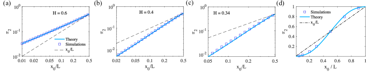
Figure 7: Same quantities as in Fig. 2(a-d) when $\pi_{2}$ is evaluated with (86) rather than with Eq. (2).

Let us now focus on the $d=2$ case, the notations describing the geometry of the targets and the initial position are specified on Supplementary Figure 8. We focus temporarily on the single target problem, focusing on target $i$. The initial position is $\mathbf{r}_{0}$ and the angle between $(\mathbf{r}_{0}-\mathbf{r}_{i})$ with respect to the $x$ axis is $\theta_{0}^{(i)}$. If the position at the target surface when the target is hit is $\mathbf{r}_{s}$, we define $\theta_{i}$ the angle between $\mathbf{r}_{s}-\mathbf{r}_{i}$ and the $x$ axis. We call $\Pi_{i}(\theta_{i})$ the pdf of $\theta_{i}$. We use the additional approximation that, after a FPT event with entrance angle $\theta_{i}$ (and entrance position $\mathbf{r}_{s}(\theta_{i})$), the average trajectory after the FPT is $\mathbf{r}_{i}+\mu_{i}(t)\hat{\mathbf{u}}(\theta)$, where $\hat{\mathbf{u}}(\theta)$ is the unit vector oriented in the direction $\theta$. Here $\mu_{i}(t)$ is assumed to be independent of $\theta_{i}$. In these conditions, in the single target problem with only target $i$, one has

$$\frac{\langle T\rangle_{i}}{V}=\int_{0}^{\infty}dt[q_{i}(\mathbf{r}^{*},t)-p(\mathbf{r}^{*},t)]=\int_{0}^{\infty}dt\left\{\int_{-\pi}^{\pi}d\theta_{i}\ \Pi_{i}(\theta_{i})\frac{e^{-\frac{[\mathbf{r}^{*}-\mu_{i}\hat{\mathbf{u}}(\theta_{i})]^{2}}{2\psi}}}{2\pi\psi(t)}-\frac{e^{-\frac{[\mathbf{r}^{*}-x_{0}\hat{\mathbf{u}}(\theta_{0}^{(i)})]^{2}}{2\psi(t)}}}{2\pi\psi(t)}\right\},$$ (89)

for any $\mathbf{r}^{*}$ inside the target. Here, $\langle T\rangle_{i}$ is the mean FPT to target $i$ in the single target problem. Taking $\mathbf{r}^{*}=a\ e_{r}(\theta^{*})$, multiplying by $\cos(\theta^{*}-\theta_{0}^{(i)})$ and integrating over $\theta^{*}$ leads

$$0=\int_{0}^{\infty}dt\int_{0}^{2\pi}d\theta^{*}\cos(\theta^{*}-\theta_{0}^{(i)})\left\{\int_{-\pi}^{\pi}d\theta_{i}\ \Pi_{i}(\theta_{i})\frac{e^{-\frac{(a^{2}+\mu_{i}^{2}-2a\mu_{i}\cos(\theta_{i}-\theta^{*})}{2\psi(t)}}}{2\pi\psi(t)}-\frac{e^{-\frac{a^{2}+x_{0}^{2}-2ax_{0}\cos(\theta^{*}-\theta_{0}^{(i)})}{2\psi(t)}}}{2\pi\psi(t)}\right\}.$$ (90)

The integration over $\theta^{*}$ leads to

$$0=\int_{0}^{\infty}dt\left\{\int_{-\pi}^{\pi}d\theta\ \Pi_{i}(\theta_{i})\frac{e^{-\frac{a^{2}+\mu_{i}^{2}}{2\psi(t)}}}{\psi(t)}\tilde{I}_{1}\left(\frac{a\mu_{i}}{\psi}\right)\cos(\theta_{i}-\theta_{0}^{(i)})-\frac{e^{-\frac{a^{2}+x_{0}^{2}}{2\psi(t)}}}{\psi(t)}\tilde{I}_{1}\left(\frac{ax_{0}}{\psi}\right)\right\},$$ (91)

where $\tilde{I}_{1}(x)=e^{-x}I_{1}(x)$, with $I_{1}$ the modified Bessel function of first kind. As a consequence, we find

$$\langle\cos(\theta_{i}-\theta_{0}^{(i)})\rangle_{\Pi_{i}}=\frac{\int_{0}^{\infty}dt\ \frac{e^{-\frac{a^{2}+x_{0}^{2}}{2\psi(t)}}}{\psi(t)}\tilde{I}_{1}\left(\frac{ax_{0}}{\psi}\right)}{\int_{0}^{\infty}dt\ \frac{e^{-\frac{a^{2}+\mu_{i}^{2}}{2\psi(t)}}}{\psi(t)}\tilde{I}_{1}\left(\frac{a\mu_{i}}{\psi}\right)}.$$ (92)

Now, we will use the ansatz

$$\Pi_{i}(\theta_{i})=\frac{e^{\alpha_{i}\cos(\theta_{i}-\theta_{0}^{(i)})}}{2\pi I_{0}(\alpha_{i})},$$ (93)

so that

$$\langle\cos(\theta-\cos\theta_{0}^{(i)})\rangle_{\Pi_{i}}=\frac{I_{1}(\alpha_{i})}{I_{0}(\alpha_{i})}.$$ (94)

As a consequence, for any position $\mathbf{r}$ so that the angle between $\mathbf{r}-\mathbf{r}_{i}$ and the $x$ axis is $\theta$, at a distance $r$ from target $i$, one has

$$q_{i}(\mathbf{r}=\mathbf{r}_{i}+r\hat{\mathbf{u}}(\theta),t)=\int_{0}^{2\pi}d\theta_{i}\Pi_{i}(\theta_{i})\frac{e^{-\frac{[r\hat{\mathbf{u}}(\theta)-\mu_{i}\hat{\mathbf{u}}(\theta_{i})]^{2}}{2\psi}}}{2\pi\psi}=\int_{0}^{2\pi}d\theta_{i}\frac{e^{\alpha_{i}\cos(\theta_{i}-\theta_{0}^{(i)})}}{2\pi I_{0}(\alpha_{i})}\times\frac{e^{-\frac{r^{2}+\mu_{i}^{2}-2r\mu_{i}\cos(\theta-\theta_{i})}{2\psi}}}{2\pi\psi}$$

$$=\int_{0}^{\infty}\frac{dt}{2\pi\psi}\frac{e^{-\frac{r^{2}+\mu_{i}^{2}}{2\psi}}\ I_{0}\left[\sqrt{\left(\alpha_{i}+\frac{r\cos(\theta-\theta_{0}^{(i)})\mu_{i}}{\psi}\right)^{2}+\left(\frac{r\sin(\theta-\theta_{0}^{(i)})\mu_{i}}{\psi}\right)^{2}}\right]}{I_{0}(\alpha_{i})}.$$ (95)

where we have used $\int_{0}^{2\pi}dte^{a\cos t+b\sin t}=2\pi I_{0}(\sqrt{a^{2}+b^{2}})$. The procedure to evaluate $\pi_{2}$ and $\langle T\rangle/V$ is the following: first, we evaluate $\mu_{1}(t)$ and $\mu_{2}(t)$ for the single target problem, see Ref. guerin16 , then we find $\alpha_{1}$ and $\alpha_{2}$ using (94) and (92), and finally we use the above expression to evaluate the $h_{ij}$ in (87) and (86).

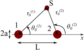
Figure 8: Notations for the geometry of the initial position and the target locations in the 2D problem.

References

(1)
Feller, W.
An Introduction to Probability Theory and Its
Applications. Vol. I (Wiley (New York),
1968).
(2)
Alfred, P. & Moran, P.
The Statistical Processes of Evolutionary
Theory (Oxford University Press, New York,
1962).
(3)
Lua, R. C. & Grosberg, A. Y.
First passage times and asymmetry of dna
translocation.
Phys. Rev. E72,
061918 (2005).
(4)
Espenson, J. H.
Chemical kinetics and reaction mechanisms,
vol. 102 (McGraw-Hill New York,
1995).
(5)
Hansen, S. D. et al.Stochastic geometry sensing and polarization in a
lipid kinase–phosphatase competitive reaction.
Proc. Natl. Acad. Sci.116, 15013–15022
(2019).
(6)
Motti, S. G. et al.Controlling competing photochemical reactions
stabilizes perovskite solar cells.
Nat. Photon.13,
532–539 (2019).
(7)
Van Kampen, N.
Stochastic Processes in Physics and Chemistry,
Third Edition (, Amsterdam, 2007).
(8)
Redner, S.
A guide to First- Passage Processes
(Cambridge University Press, Cambridge, England,
2001).
(9)
Dobramysl, U. & Holcman, D.
Triangulation sensing to determine the gradient
source from diffusing particles to small cell receptors.
Phys. Rev. Lett.125, 148102
(2020).
(10)
Cheviakov, A. F. & Ward, M. J.
Optimizing the principal eigenvalue of the laplacian
in a sphere with interior traps.
Math. Comp. Modelling53, 1394–1409
(2011).
(11)
Bressloff, P. C.
Target competition for resources under multiple
search-and-capture events with stochastic resetting.
Proc. Royal Soc. A476, 20200475
(2020).
(12)
Bressloff, P. C.
First-passage processes and the target-based
accumulation of resources.
Phys. Rev. E103, 012101
(2021).
(13)
Condamin, S., Bénichou, O. &
Moreau, M.
Random walks and brownian motion: A method of
computation for first-passage times and related quantities in confined
geometries.
Phys. Rev. E75,
021111 (2007).
(14)
Condamin, S. & Bénichou, O.
Exact expressions of mean first-passage times and
splitting probabilities for random walks in bounded rectangular domains.
J. Chem. Phys.124, 206103
(2006).
(15)
Condamin, S., Bénichou, O. &
Moreau, M.
First-passage times for random walks in bounded
domains.
Phys Rev Lett95, 260601
(2005).
(16)
Condamin, S., Tejedor, V.,
Voituriez, R., Bénichou, O. &
Klafter, J.
Probing microscopic origins of confined subdiffusion
by first-passage observables.
Proc. Natl. Acad. Sci.105, 5675–5680
(2008).
(17)
Bénichou, O. & Voituriez, R.
From first-passage times of random walks in
confinement to geometry-controlled kinetics.
Phys. Rep.539,
225–284 (2014).
(18)
Majumdar, S. N., Rosso, A. &
Zoia, A.
Hitting probability for anomalous diffusion
processes.
Phys. Rev. Lett.104, 020602
(2010).
(19)
Wiese, K. J.
First passage in an interval for fractional brownian
motion.
Phys. Rev. E99,
032106 (2019).
(20)
Bouchaud, J.-P., Bonart, J.,
Donier, J. & Gould, M.
Trades, quotes and prices: financial markets
under the microscope (Cambridge University Press,
2018).
(21)
Richard, D. & Speck, T.
Crystallization of hard spheres revisited. i.
extracting kinetics and free energy landscape from forward flux sampling.
J. Chem. Phys.148, 124110
(2018).
(22)
Oshanin, G. & Redner, S.
Helix or coil? fate of a melting heteropolymer.
EPL85,
10008 (2009).
(23)
Lubensky, D. K. & Nelson, D. R.
Single molecule statistics and the polynucleotide
unzipping transition.
Phys. Rev. E65,
031917 (2002).
(24)
Best, R. B. & Hummer, G.
Reaction coordinates and rates from transition
paths.
Proc. Natl. Acad. Sci.102, 6732–6737
(2005).
(25)
Chodera, J. D. & Pande, V. S.