Deep Reinforcement Learning with Dynamic Graphs
for Adaptive Informative Path Planning

Abstract

Autonomous robots are often employed for data collection due to their efficiency and low labour costs. A key task in robotic data acquisition is planning paths through an initially unknown environment to collect observations given platform-specific resource constraints, such as limited battery life. Adaptive online path planning in 3D environments is challenging due to the large set of valid actions and the presence of unknown occlusions. To address these issues, we propose a novel deep reinforcement learning approach for adaptively replanning robot paths to map targets of interest in unknown 3D environments. A key aspect of our approach is a dynamically constructed graph that restricts planning actions local to the robot, allowing us to quickly react to newly discovered obstacles and targets of interest. For replanning, we propose a new reward function that balances between exploring the unknown environment and exploiting online-collected data about the targets of interest. Our experiments show that our method enables more efficient target detection compared to state-of-the-art learning and non-learning baselines. We also show the applicability of our approach for orchard monitoring using an unmanned aerial vehicle in a photorealistic simulator.

I Introduction

Efficient data collection is a key requirement in many monitoring tasks, such as environmental mapping [1, 2, 3, 4, 5], precision agriculture [6, 7, 8], and exploration [9, 10, 11]. Autonomous robots are becoming popular tools for mobile sensing applications since they offer labour- and cost-effective alternatives to using conventional platforms, manual approaches [12], or static sensing methods [13]. A key challenge in this context is planning paths that maximise the information value of collected data in large environments with limited onboard resources, e.g. mission time or battery capacity.

In this work, our goal is to map a set of targets of interest in an initially unknown 3D environment using an unmanned aerial vehicle (UAV) with a unidirectional sensor as efficiently as possible. Possible applications for such a system are finding apples in an orchard, victims in a search and rescue scenario, or components in a warehouse. We cast this problem as the informative path planning problem, which aims to maximise the information value of obtained sensor observations subject to resource constraints, e.g. maximum path length or battery capacity. Our problem considers adaptively replanning robot paths to account for observations collected online. In our setting, adaptive replanning is challenging due to the presence of unknown view-dependent occlusions in the environment and planning in a 4D action space, i.e. the UAV 3D position and yaw angle.

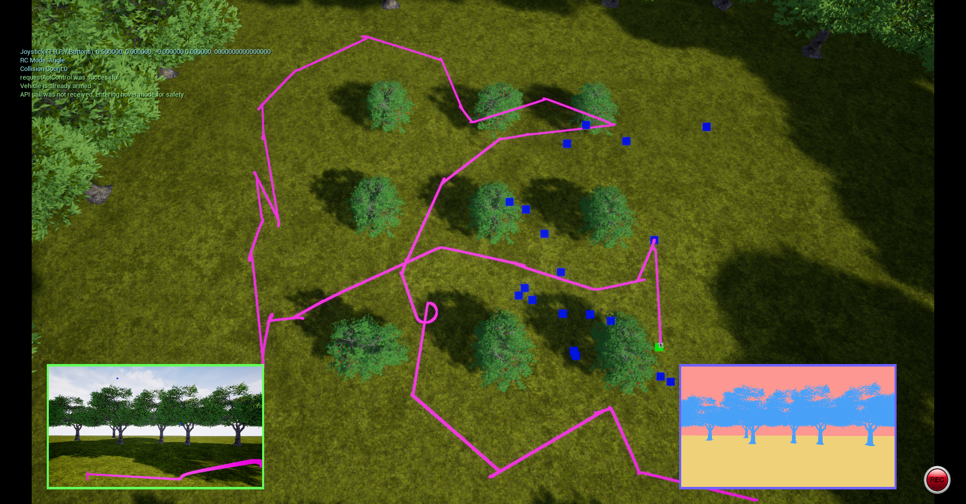
Figure 1: Our reinforcement learning approach for adaptive informative path planning applied in an orchard monitoring scenario using an unmanned aerial vehicle (UAV). Blue squares are candidate waypoints output by our planner, while the green square is the chosen next waypoint to visit. The inset windows show the onboard camera view and semantic segmentation for apple detection. By planning collision-free paths for the UAV online, we maximise the number of apple fruits detected under flight time constraints.

Classical approaches for 3D model acquisition precompute a path before the mission starts [14, 15, 9]. The robot does not reason about and thus cannot adapt its behaviour to new observations gathered during the mission via online replanning. In contrast, adaptive informative path planning approaches allow robots to replan their paths online based on newly collected data [10, 16, 17, 18, 19, 20]. However, these methods are typically computationally inefficient in complex environments involving high-dimensional action spaces, such as those found in UAV-based applications. Recently, approaches using deep reinforcement learning have been proposed for adaptive informative planning that outperform non-learning methods in various scenarios [21, 22, 23, 24]. However, current reinforcement learning-based methods are not directly applicable to our problem setting as they do not consider adjusting the sensor orientation [23, 22, 21] or assume obstacle-free workspaces [24, 22]. Extending existing approaches for obstacle avoidance is non-trivial as it involves updating the robot action space as the obstacles are discovered.

The main contribution of this paper is a deep reinforcement learning-based approach for adaptive replanning in unknown 3D environments to maximise the detected targets of interest. A key aspect of our approach is a dynamically constructed graph to represent the action space which supports sequentially selecting the next best waypoint for the robot to visit. Our dynamic graph restricts planning to actions in the robot’s local region at each timestep of the mission. Updating the action space in this way enables us to plan informative collision-free paths, even without prior knowledge about the environment. This is in contrast to previous works [22, 16, 10] which reason about a static, predefined representation of the action space. Combining our dynamic graph with sequential decision-making through reinforcement learning allows us to plan long-horizon paths. To capture the adaptive informative planning objective, we propose a new reward function that encourages the robot to both explore unknown regions and exploit detected targets. We demonstrate the performance of our approach by evaluating the percentage of targets detected during the mission, showing that it outperforms baselines. Fig. 1 exemplifies our approach applied on a UAV to detect fruits in an orchard.

In sum, we make the following three claims. First, our approach enables more efficiently detecting targets of interest compared to state-of-the-art non-learning-based and learning-based planning methods, including in previously unseen environments. Second, by adapting the action space online, our dynamic graph ensures collision-free navigation in initially unknown environments while performing on par with or outperforming static global representations. Third, our proposed reward function outperforms using purely exploratory rewards. We validate the performance of our approach in a realistic orchard monitoring scenario using a UAV. We open-source our code and provide a pre-trained model for the community at: https://github.com/dmar-bonn/ipp-rl-3d.

II Related Work

Informative path planning has been extensively applied in exploration and monitoring tasks using robotic systems. Classical approaches [14, 15, 9, 20] either plan a path offline before a mission starts or optimise paths to cover the complete robot workspace [25]. These combinatorial methods do not allow for online replanning due to the large computational burden incurred when exhaustively evaluating all possible paths through the environment. Hence, these approaches are not applicable to our problem setting.

A common strategy for reducing computational complexity is discretising the continuous action space for planning by sampling and interconnecting candidate waypoints through platform-dependent paths. The robot is constrained to visit only the set of sampled waypoints and travel only over the predefined paths. The waypoints and paths form a static global graph representing the entire environment. Recent approaches [26, 27, 28] incrementally add waypoints based on the current robot pose to construct the global graph, leading to reduced replanning time. However, similar to classical approaches, these methods are inherently non-adaptive and do not consider previously collected observations for online path replanning during a mission.

Adaptive informative path planning approaches [10, 18, 19, 16, 29, 30, 31, 32, 33, 4, 17] replan robot paths online and consider gathered observations to inform subsequent decision steps. Several studies apply evolutionary algorithms to optimise paths for UAVs [31, 17, 34] or autonomous surface vehicles [10] in a receding-horizon manner, allowing for adaptive online replanning. Ercolani et al. [16] consider gas distribution mapping using a nano aerial vehicle. They separate path planning into global and local stages by clustering the sampled waypoints and planning over clusters instead of individual waypoints. Similarly, Lim et al. [18] form clusters by solving a group Steiner problem and frame adaptive informative planning for a UAV as a travelling salesman problem through the clustered regions. Oßwald et al. [35] combine globally optimal travelling salesman problem solutions on a coarse scale with effective local exploration adapting to the environment. In contrast to our work, they consider obstacle-free workspaces. To cater for the mapping uncertainty in UAV-based monitoring, Rückin et al. [4] and Mascarich et al. [29] derive information-theoretic measures to guide the planning objective. However, these works also assume obstacle-free workspaces. Schmid et al. [19] propose new techniques for node rewiring in sampling-based path planning strategies utilising a point sensor. They do not consider planning for unidirectional sensors in contrast to our work. In general, a major limitation of adaptive methods involving replanning is the need to evaluate the information value for multiple candidate paths online, which incurs high computational costs over long planning horizons in complex environments.

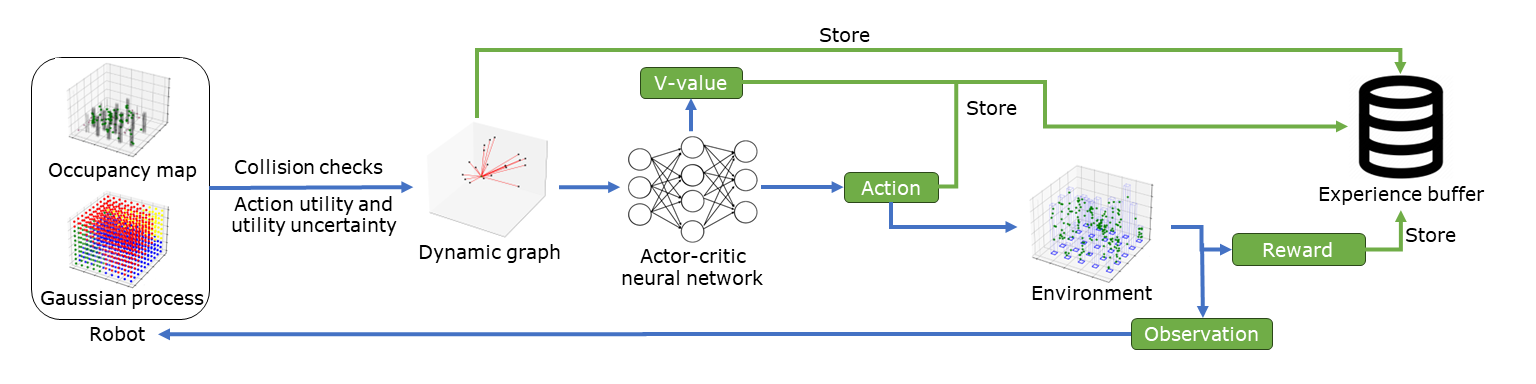
Figure 2: At each mission timestep $t$, our approach samples collision-free waypoints in the robot’s local environment. These waypoints, with considered yaw directions, generate action nodes. Each action node is associated with utility value and uncertainty of the utility value, regressed from the Gaussian process, to generate the dynamic graph. Our actor-critic network uses the dynamic graph to output the robot’s state value and predicts the next action to execute, which generates a reward and observations from the environment. Blue arrows indicate the robot control loop and green indicate variables stored in the experience buffer to train the actor-critic network via on-policy learning.

Recent studies combine neural networks and reinforcement learning to solve the informative path planning problem [24, 23, 22, 36, 21]. Reinforcement learning-based solutions offer the benefits of computational efficiency at deployment and the ability to generalise to similar environments not seen during training. While Rückin et al. [24] combine Monte Carlo tree search with a convolutional neural network, Choi and Cielniak [23] consider advantages of paths planned by multiple low-level controllers. Cao et al. [22] propose an attention-based neural network to achieve context-aware path planning in 2D workspaces, whereas Wei and Zheng [21] use recurrent neural networks trained with Q-learning to plan the path. However, these methods are not directly applicable to our problem setup as they do not consider obstacle avoidance [24, 23, 22, 21], are constrained to specific information distributions, e.g. 2D Gaussian fields [22], or do not account for unidirectional sensors [23, 22, 21]. Our approach is most similar to the one of Cao et al. [22], which plans over a probabilistic roadmap-based environment representation in obstacle-free 2D workspaces. A key difference with respect to their work is that we introduce a dynamic graph action space which supports unknown obstacles in 3D workspaces, as required for UAV-based applications. Moreover, our proposed reward function not only encourages exploratory behaviour, as commonly done in previous studies [22, 21] but also incentivises exploiting newly collected information. We show that the policy learned on our new reward function outperforms the one learned on purely exploratory rewards.

III Our approach

We propose a novel deep reinforcement learning-based informative path planning approach for maximising the number of detected targets of interest in unknown 3D environments. Fig. 2 overviews our method. A key aspect of our approach is a graph that restricts planning to actions in the robot’s local workspace, allowing us to generate collision-free paths. We call this technique of representing the environment a dynamic graph since it evolves to account for newly gathered observations. For each action, we define a utility value as the number of targets observed upon executing it. We utilise a Gaussian process to capture the relationship between utility values associated with actions. We regress the utility value and its corresponding uncertainty from the Gaussian process for each action in the current dynamic graph. At each timestep, our policy network outputs a probability distribution over the actions in the dynamic graph. We use the obtained observations to train the Gaussian process and generate rewards reflecting the informative planning objective. The observations are also utilised to update the occupancy map in the realistic simulation. We develop a new reward function that considers both the reduction in utility uncertainty and the number of observed targets. An experience buffer collects the robot’s dynamic graph, sampled action, predicted state value, and reward over several training episodes to train the actor-critic network using on-policy reinforcement learning.

III-A Environment Modelling

Our aim is to map the distribution of targets of interest in a 3D environment with unknown obstacles. We use Gaussian processes to model the view-dependent number of observed targets. We also maintain an occupancy map to plan collision-free paths. Our mission budget $B\in\mathbb{R}^{+}$ is defined as the maximum cost of the traversed path. We define the robot workspace as a set $\mathcal{A}$ of actions $\mathbf{a}_{i}=[x_{i},y_{i},z_{i},d_{i}]^{\top}$, where $x_{i},y_{i},z_{i}\in\mathbb{R}$ are the robot 3D position coordinates within environment bounds and $d_{t}\in\mathcal{D}$ is the yaw of the unidirectional onboard sensor, such as an RGB or RGB-D camera. An action represents the next robot pose. The robot takes observations at each distance interval $h$ as it travels. The set $\mathcal{D}$ denotes a user-defined set of possible robot yaw directions. During planning, at each mission timestep $t$, we plan over a set of $L$ candidate actions in the set $\mathcal{A}_{t}\subseteq\mathcal{A},~{}|\mathcal{A}_{t}|=L$. The candidate actions are sampled uniformly at random from the $C$-neighbourhood around $\mathbf{a}_{t-1}$, where $C$ is a constant specifying the extent of the robot’s local region.

After executing an action $\mathbf{a}_{t}$, the robot observes a certain number of targets. We define the utility function $u:\mathcal{A}\rightarrow\mathbb{R}^{+}$ as mapping action $\mathbf{a}_{t}$ to the observed number of targets. The observed targets for $u$ are normalised by the total number of targets in the environment to ensure normalised neural network input features for stable policy training.

Gaussian processes are widely used to represent spatially correlated phenomena [37, 21, 10, 22]. We use a Gaussian process to predict the candidate actions’ utility values and associated variances. The Gaussian process is trained on the utility values of the actions executed in the past. We exploit the Gaussian process to inform the policy. The variance allows our policy to consider the uncertainty in predicted utility values during planning.

A Gaussian process is characterised by a mean function $m(\mathbf{a}_{i})\triangleq\mathbb{E}[u(\mathbf{a}_{i})]$ and a covariance function $k(\mathbf{a}_{i},\mathbf{a}_{i}^{\prime})\triangleq\mathbb{E}[(u(\mathbf{a}_{i})-m(\mathbf{a}_{i}))(u(\mathbf{a}_{i}^{\prime})-m(\mathbf{a}_{i}^{\prime}))]$ as $u(\mathbf{a}_{i})\sim GP(m(\mathbf{a}_{i}),k(\mathbf{a}_{i},\mathbf{a}_{i}^{\prime}))$, where $\mathbb{E}[\cdot]$ is the expectation operator and $\mathbf{a}_{i},\mathbf{a}_{i}^{\prime}\in\mathcal{A}$. Hence, considering a set of candidate actions $\mathcal{A}_{t}$ at timestep $t$ for which we wish to infer the utility, let the actions in set $\mathcal{A}_{t}$ correspond to a feature matrix $\mathbf{A}_{t}$, where each $i^{th}$ row corresponds to the action vector $\mathbf{a}_{t}^{i}\in\mathcal{A}_{t}$. The set of all previously executed actions $\{\mathbf{a}_{0},\mathbf{a}_{2},\ldots,\mathbf{a}_{t-1}\}$ is represented by feature matrix $\mathbf{A}_{t-1}^{\prime}$. Utility values corresponding to previously executed actions are represented by the vector $\mathbf{u}_{t-1}^{\prime}=[u(\mathbf{a}_{1}),\ldots,u(\mathbf{a}_{t-1})]^{\top}$. We predict the utility values of candidate action set $\mathcal{A}_{t}$ by conditioning the Gaussian process on the observed utility values $\mathbf{u}_{t}\mid\mathbf{A}_{t-1}^{\prime},\mathbf{u}_{t-1}^{\prime},\mathbf{A}_{t}\sim\mathcal{N}(\boldsymbol{\upmu},\mathbf{P})$:

$$\boldsymbol{\upmu}(\mathbf{A}_{t},\mathbf{A}_{t-1}^{\prime})={} \mathbf{m}(\mathbf{A}_{t})+\mathbf{K}(\mathbf{A}_{t},\mathbf{A}_{t-1}^{\prime})\,[\mathbf{K}(\mathbf{A}_{t-1}^{\prime},\mathbf{A}_{t-1}^{\prime})$$

$$+\sigma_{n}^{2}\mathbf{I}]^{-1}\big{(}\mathbf{u}_{t-1}^{\prime}-\mathbf{m}(\mathbf{A}_{t-1}^{\prime})\big{)}\,\textrm{,}$$ (1)

$$\mathbf{P}(\mathbf{A}_{t},\mathbf{A}_{t-1}^{\prime})={} \mathbf{K}(\mathbf{A}_{t},\mathbf{A}_{t})-\mathbf{K}(\mathbf{A}_{t},\mathbf{A}_{t-1}^{\prime})[\mathbf{K}(\mathbf{A}_{t-1}^{\prime},$$

$$\mathbf{A}_{t-1}^{\prime})+\sigma_{n}^{2}\mathbf{I}]^{-1}\mathbf{K}(\mathbf{A}_{t},\mathbf{A}_{t-1}^{\prime})^{\top}\,\textrm{,}$$ (2)

where $\sigma_{n}^{2}\in\mathbb{R}^{+}$ is a hyperparameter describing the measurement noise variance, $\mathbf{I}$ is an $n\times n$ identity matrix where $n=t-1$, and $\mathbf{K}(\cdot,\cdot)$ corresponds to the covariance matrix.

III-B Adaptive Informative Path Planning

We model the path followed by the robot as a sequence of consecutively executed actions $\psi_{0}^{T}=(\mathbf{a}_{0},\mathbf{a}_{1},\ldots,\mathbf{a}_{T})$ where $\mathbf{a}_{0}$ denotes the start action, i.e. the initial robot pose, and $\mathbf{a}_{T}$ is the final action which depletes the budget $B$. The general informative path planning problem aims to find an optimal path ${\psi^{\ast}}_{0}^{T}\in\Psi$ in the space of all possible paths $\Psi$ to optimise an information-theoretic objective function:

$${\psi^{\ast}}_{0}^{T}=\mathop{{\rm{argmax}}}\limits_{\psi\in\Psi}~{}{\rm\mathit{I}}(\psi),\ {\rm{s.t.}}\,\,C(\psi)\leq B\,,$$ (3)

where ${\rm\mathit{I}}:\psi_{0}^{T}\xrightarrow{}\mathbb{R}^{+}$ is the information gained from observations obtained along path $\psi_{0}^{T}$, the cost function ${C}:\psi_{0}^{T}\xrightarrow{}\mathbb{R}^{+}$ maps path $\psi_{0}^{T}$ to its execution cost.

Our robot traverses a straight line between two consecutive actions. Observations are equidistantly collected along the path $\psi_{0}^{T}$ at a frequency $h$. An observation is used to update the Gaussian process and generate a reward. Hence, we model the informative path planning problem as a sequential decision-making process. As we aim to maximise the number of observed targets, we define a function $\nu:\mathcal{A}\times\Psi\rightarrow\mathbb{R}^{+}$ as the number of new targets observed upon executing an action $\mathbf{a}_{t}\in\mathcal{A}$ after following the path $\psi_{0}^{t-1}$. Note that information $\nu(\mathbf{a}_{t},\psi_{0}^{t-1})$ and utility $u(\mathbf{a}_{t})$ differ as the utility measures the number of all targets observed upon executing an action, whereas information considers only targets that were newly observed after executing the action. Hence, modelling $\nu(\mathbf{a}_{t},\psi_{0}^{t-1})$ with a Gaussian process would require including the temporal variations of an action’s utility value, increasing the Gaussian process and policy training complexity. We therefore choose to model utility with a Gaussian process, as it only depends on a single action $\mathbf{a}_{t}$.

We define the information obtained along a path as:

$$\mathit{I}(\psi_{0}^{T})=\sum_{t=1}^{T}\,\nu(\mathbf{a}_{t},\psi_{0}^{t-1})\,,$$ (4)

where we aim to plan a path $\psi_{0}^{T}$ to maximise information $\mathit{I}$.

For informative planning, we leverage our Gaussian process defined in Sec. III-A to regress the utility and variance associated with actions. We apply an upper confidence bound to the set of candidate actions $\mathcal{A}_{t}$ to obtain a subset of high-interest actions $\hat{\mathcal{A}_{t}}$ used in our reward function:

$$\hat{\mathcal{A}_{t}}=\{\mathbf{a}_{i,t}\in\mathcal{A}_{t}\,|\,m(\mathbf{a}_{i,t})+\beta k(\mathbf{a}_{i,t},\mathbf{a}_{i,t})\geq\mu_{th}\}\,,$$ (5)

where $m(\mathbf{a}_{i,t})$ and $k(\mathbf{a}_{i,t},\mathbf{a}_{i,t})$ are the mean utility of action $\mathbf{a}_{i,t}$ and corresponding variance inferred from the Gaussian process. The parameter $\beta\in\mathbb{R}$ controls the confidence interval width and $\mu_{th}$ is a user-defined threshold.

We introduce a new reward function that balances exploring the environment and exploiting collected information. The information criteria in previous works [22, 21] consider environment exploration only. However, our problem considers detecting targets, therefore requiring a measure of information value in the reward. At each timestep $t$, the robot executes action $\mathbf{a}_{t}$, collects observations and receives a reward $r_{t}\in\mathbb{R}^{+}$. Our reward function consists of an exploration term $r_{e,t}$ and an information term $r_{u,t}$:

$$\begin{split}r_{t}(\hat{\mathbf{A}}_{t},\mathbf{A}_{t-1}^{\prime},\mathbf{A}_{t}^{\prime},\mathbf{a}_{t},\psi_{0}^{t-1})&=\\ \,\alpha r_{e,t}(\hat{\mathbf{A}}_{t},\mathbf{A}_{t-1}^{\prime},&\mathbf{A}_{t}^{\prime})+\,\beta r_{u,t}(\mathbf{a}_{t},\psi_{0}^{t-1})\,,\\ \end{split}$$ (6)

with:

$$\begin{split}r_{e,t}(\hat{\mathbf{A}}_{t},\mathbf{A}_{t-1}^{\prime},\mathbf{A}_{t}^{\prime})=&\frac{\operatorname{Tr}(\mathbf{P}(\hat{\mathbf{A}}_{t},\mathbf{A}_{t-1}^{\prime}))-\operatorname{Tr}(\mathbf{P}(\hat{\mathbf{A}}_{t},\mathbf{A}_{t}^{\prime}))}{\operatorname{Tr}(\mathbf{P}(\hat{\mathbf{A}}_{t},\mathbf{A}_{t-1}^{\prime}))}\,,\\ r_{u,t}(\mathbf{a}_{t},\psi_{0}^{t-1})=&\nu(\mathbf{a}_{t},\psi_{0}^{t-1})\,,\\ \end{split}$$ (7)

where $\operatorname{Tr}(\cdot)$ is the trace operator of a matrix and $\alpha$ and $\beta$ are constants used to trade off exploration and exploitation.

The variance reduction of the Gaussian process measures exploration $r_{e,t}$. To this end, we maximise the decrease in the covariance matrix trace following the A-optimal design criterion [38]. Scaling the reward by $\operatorname{Tr}(P(\hat{\mathbf{A}}_{t},\mathbf{A}_{t-1}^{\prime}))$ stabilises the actor-critic network training [22]. The term $r_{u,t}$ measures the new information gained after executing $\mathbf{a}_{t}$.

III-C Dynamic Graph Representation

Adaptive informative path planning requires reasoning about the information distribution in the environment. We propose a dynamic graph that models the collision-free action space and information distribution in the robot’s neighbourhood by sampling actions as defined in Sec. III-A, as opposed to a static global non-obstacle-aware representation [22, 16, 10]. Our dynamic graph efficiently represents the current knowledge about the environment, which the robot’s policy uses to predict the next action (Sec. III-D).

At each timestep $t$, we (re-)build a fully connected graph $\mathcal{G}_{t}=(\mathcal{N}_{t},\mathcal{E}_{t})$, where the node set $\mathcal{N}_{t}$ is the set of candidate actions $\mathcal{A}_{t}$ defined in Sec. III-A, to account for newly gathered observations. We randomly sample $K$ candidate positions $[x_{i},y_{i},z_{i}]^{\top}$ within a $C$-neighbourhood of the current robot position and create $L=K\times|\mathcal{D}|$ nodes by associating each position with possible yaws $\mathcal{D}$. The edge set $\mathcal{E}_{t}$ connects each pair of actions such that $e_{i,j,t}=(i,j,c_{i,j})\in\mathcal{E}_{t}$, where the cost $c_{i,j}$ is the edge weight, $i,j\leq L$, and $i\neq j$. The cost $c_{i,j}$ is the sum of the actions’ Euclidean distance and a small constant cost $C_{s}$ if the robot yaw changes.

To better inform the planning policy, we leverage our Gaussian process to create node features utilised in our actor-critic network. At each timestep $t$, the node feature matrix $\mathbf{M}_{t}$ of graph $\mathcal{G}_{t}$ consists of the robot’s candidate actions and the mean and variance values queried from the Gaussian process. The $i^{\mathrm{th}}$ row of $\mathbf{M}_{t}$ relates to the $i^{\mathrm{th}}$ action:

$$\mathbf{M}_{t}(i)=[\mathbf{a}_{i,t},\,m(\mathbf{a}_{i,t}),\,k(\mathbf{a}_{i,t},\mathbf{a}_{i,t})]\,,$$ (8)

where $\mathbf{a}_{i,t}=[x_{i,t},\,y_{i,t},\,z_{i,t},\,d_{i,t}]^{\top}$, and $m(\mathbf{a}_{i,t})$ and $k(\mathbf{a}_{i,t},\mathbf{a}_{i,t})$ are the regressed action’s utility and variance.

III-D Actor-Critic Neural Network for Reinforcement Learning

We exploit the dynamic graph to model collision-free actions for the planning policy to reason about and represent the current knowledge about the information distribution in the environment. As the Gaussian process only predicts the utility of greedily executing a single next action, we use reinforcement learning to train our policy for informative path planning over long-horizon paths.

We use an attention-based neural network to parameterise our stochastic planning policy $\pi(\mathcal{G}_{t},\psi_{0}^{t-1},B_{r},\mu_{th})\in[0,1]^{L}$ that predicts a probability distribution over all actions $\mathcal{A}_{t}$ based on the current dynamic graph $\mathcal{G}_{t}$, previously executed path $\psi_{0}^{t-1}$, remaining budget $B_{r}$, and the mean threshold $\mu_{th}$ defining actions of interest in Eq. 5. We follow the network structure proposed by Cao et al. [22] consisting of an encoder and a decoder module. The attention-based encoder learns the dependencies between actions in $\mathcal{G}_{t}$. We condition the learned actions’ latent dependencies on a planning state consisting of previously executed actions $\psi_{0}^{t-1}$, the remaining budget $B_{r}$, and the threshold $\mu_{th}$. A budget mask filters out actions not reachable within the remaining budget. Based on the conditioned latent action dependencies, a decoder outputs a probabilistic policy reasoning over all actions in the dynamic graph. During training, the decoder also estimates the value function $V(\mathcal{G}_{t},\psi_{0}^{t-1},B_{r},\mu_{th})~{}\in~{}\mathbb{R}$ following the current policy $a_{t}\sim\pi(\mathcal{G}_{t},\psi_{0}^{t-1},B_{r},\mu_{th})$. The estimated values, sampled actions, dynamic graphs, planning states, and rewards are stored in the experience buffer utilised to train the policy with an on-policy actor-critic reinforcement algorithm. In this work, we use proximal policy optimisation [39]. During deployment, we choose the most informative action:

$$\mathbf{a}_{t}=\mathop{{\rm{argmax}}}\limits_{\mathbf{a}_{i,t}\in\mathcal{A}_{t}}{\pi(\mathcal{G}_{t},\psi_{0}^{t-1},B_{r},\mu_{th})_{i}}\,.$$ (9)

IV Experimental Results

We experimentally validate our three claims on the task of UAV-based fruit monitoring in apple orchards. First, our approach enables more efficiently detecting targets of interest compared to non-learning baselines and reinforcement learning-based methods. Second, our dynamic graph action space enables collision-free path planning in initially unknown environments while performing on par with state-of-the-art static global graph representations. Third, our new reward function more effectively manages the exploration-exploitation trade-off compared to using purely exploratory rewards, leading to more efficient targeted mapping. We demonstrate the performance of our approach in a realistic orchard simulation, showcasing its applicability for a practical monitoring task in a previously unseen environment.

IV-A Experimental Setup

Environment. Our environment consists of trees and fruits bounded in a scale-agnostic unit cube. We maintain an occupancy map with $50\times 50\times 50$ voxels. In the test phase, trees are generated at random positions in the environment. During training, they are arranged in a regularly spaced $5\times 5$ array. Fig. 3 shows examples of a training and a testing environment. In both cases, fruits are attached to generated trees at random positions. The occupancy grid map of the environment is initialised as unknown space and is updated via sensor observations with free space, observed fruits, and trees. For each observation, the utility value is used to train the Gaussian process detailed in Sec. III-A. We tune the hyperparameters in a small representative environment using the Matérn $1/2$ kernel with $\mu_{th}=0.4$ and $\beta=1$ in Eq. 5. For our reward function defined in Eq. 3, we set $\alpha=1.0$ and $\delta=0.01$ to keep values of both terms numerically similar to balance between exploration and exploitation.

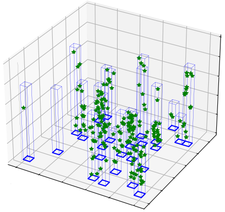
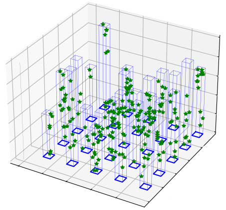
Figure 3: Examples of testing and training orchard environments used in our experiments. Left: Testing environment with trees placed at random locations. Right: Training environment with trees placed in a regular square array. Thin and dark blue lines represent tree outlines and tree bases, respectively. Green stars indicate fruits.

We consider a UAV platform with an onboard camera of $90^{\circ}$ field of view (FoV). Since the confidence in detected targets decreases with distance, we constrain the maximum detection range to 24$\%$ of environment dimension in any direction. A tree or fruit is detected only when it is within the camera range and FoV. The UAV can choose between yaw angles of $[0,\frac{\pi}{2},\pi,\frac{3\pi}{2}]$ rad at the current altitude. Note that our method can be easily extended to finer discretisations.

Training An episode consists of a UAV mission with a budget $B$. We train in a grid-based environment as a randomly initialised policy learns efficiently from this structure and transfers to randomised test environments. The number of fruits present in an environment varies between $200$ and $250$. We fix the number of positions $K$ in the dynamic graph and set the initial UAV pose to $[0,0,0,\frac{\pi}{2}]^{\top}$. To keep our policy scale-agnostic, we normalise the robot’s internal environment representation and action coordinates. Hence, the budget $B$ is unitless and real-valued, randomly generated for each episode within the range $[7,9]$. We fuse an observation into the occupancy map and Gaussian process each time the UAV travels $0.2$ units from the position of the previously obtained observation.

TABLE I: Comparison of our approach against baselines in a UAV-based fruit monitoring scenario. Our dynamic graph-based reinforcement learning approach outperforms learning and non-learning baselines while maintaining low replanning time.

Baseline	$\%$ targets	Time (s)
Our approach ($K=20$)	$65.49\pm 6.23$	$1.58$
CAtNIPP (g.)	$56.49\pm 7.65$	$1.28$
CAtNIPP (ts.)	$57.14\pm 7.60$	$44.51$
Random agent	$44.33\pm 12.15$	$1.54$
RIG-tree (Re.H.)	$44.06\pm 9.13$	$53.64$

Figure 4: Comparison of our approach against baselines in a UAV-based fruit monitoring scenario. Solid lines indicate means over 500 trials and shaded regions show standard deviations. In our approach, using our exploration-exploitation reward function with a dynamic graph action space for reinforcement learning enables more efficiently detecting targets of interest (fruit) during a mission.

We terminate an episode if the maximum number of executed actions exceeds $256$. To speed up training, we run $12$ environments in parallel. The policy is trained for $8$ epochs using a batch size of $64$ and the Adam optimiser with a learning rate of $10^{-4}$, which decays by a factor of $0.96$ each $32$ optimisation steps. The policy gradient epsilon-clip parameter is set to $0.2$. Our model is trained on a workstation equipped with an Intel(R) Xeon(R) W-2133 CPU @ 3.60GHz and one NVIDIA Quadro RTX 5000 GPU. Our policy is trained for $\sim 440,000$ environment interactions.

IV-B Comparison Against Baselines

The first set of experiments shows that our dynamic graph-based reinforcement learning approach outperforms state-of-the-art baselines. We generate $25$ test environments corresponding to different random seeds and run $20$ trials on each environment instance with a budget of $10$ units.

For our approach, we consider $K=20$ sampled waypoints, $L=80$ nodes in the dynamic graph, and the reward function described in Eq. 3. The reinforcement learning-based baseline for evaluation is CAtNIPP [22], the state-of-the-art approach closest to our work which uses global graph-based planning. Since CAtNIPP considers obstacle-free environments and modifying its global graph to account for unknown obstacles is a non-trivial task, we allow the UAV to pass through obstacles to ensure a fair comparison.

We compare against: (i) CAtNIPP with a zero-shot policy (CAtNIPP g.) where the highest probability action is executed; (ii) CAtNIPP with a trajectory sampling policy [22] (CAtNIPP ts.) where four $8$-step paths are planned and the path with highest uncertainty reduction is executed for $3$ steps; (iii) a random policy on $K=20$ dynamic graph construction (random agent); and (iv) non-learning rapidly exploring random information gathering trees [26] applied in a receding-horizon manner (RIG-tree Re.H.). To evaluate planning performance, we measure the percentage of detected targets of interest (apples) during the test. We also report average replanning time per step.

(a) CAtNIPP (g.)

(b) Our approach

Figure 5: Comparison of paths planned by (a) the global graph-based CAtNIPP [22] baseline and (b) our dynamic graph-based reinforcement learning approach with $K=20$ in a fruit monitoring scenario. The blue line shows the executed UAV path, with the brown and pink circles indicating start and end positions. Red dots are targets not yet observed, while green stars are observed targets.

Fig. 4 and Table I illustrate our results. Our approach outperforms all baselines by a significant margin. This can be attributed to the new reward function that balances between exploring the environment and exploiting collected information. Both CAtNIPP variants perform worse than our method since they only focus on utility variance reduction. In Table I, the approaches using reinforcement learning require significantly less replanning time than non-learning methods, justifying the use of learning-based strategies. Our proposed approach is more compute-efficient than CAtNIPP (ts.), and almost as efficient as CAtNIPP (g.), which facilitates its deployment in real-world scenarios.

Fig. 5 qualitatively compares the paths planned by our approach and CAtNIPP g. for the ground truth environment illustrated in Fig. 3. The visualisations correspond to paths executed at $50\%$ of the budget. Our approach favours actions that discover more targets. This is because CAtNIPP considers a purely exploratory objective, assuming a continuous distribution of utility, which leads to re-observing the high-interest regions in an oscillatory manner. Our approach does not encounter this issue. Since we both reduce uncertainty and maximise the number of discovered targets using our reward function, we obtain a more widespread distribution of observations in the environment.

IV-C Ablation Studies

Next, we systematically study the impact of our dynamic graph action space and proposed reward function on the informativeness of the planned paths to demonstrate their benefits. Our test environment is the same as in Sec. IV-B. We compare our approach against CAtNIPP [22], which uses a static graph action space based on probabilistic roadmaps and a purely exploratory reward function.

TABLE II: Graph structure ablation study. All methods use our proposed exploration-exploitation reward. The dynamic graph structure performs slightly better than the global representation of CAtNIPP.

Graph structure	$\%$ targets
$K=10$	$60.85\pm 7.51$
$K=20$	$65.49\pm 6.23$
$K=30$	$64.20\pm 6.62$
$K=40$	$66.53\pm 6.28$
$K=50$	$64.20\pm 6.80$
CAtNIPP [22]	$63.27\pm 6.89$

TABLE III: Reward function ablation study. Both dynamic graph- and global graph-based policies trained on our reward function outperform those learned on a purely exploratory reward.

Model and reward function	$\%$ targets
$K=20$, exploration	$54.75\pm 7.66$
$K=20$, our reward	$65.49\pm 6.23$
CAtNIPP [22], our reward	$63.27\pm 6.89$
CAtNIPP [22], exploration	$56.52\pm 8.29$

Graph Structure. We compare our approach using dynamic graph action spaces with different numbers of sampled waypoints $K=\{10,\,20,\,30,\,40,\,50\}$ against CAtNIPP. We use our new reward function described in Eq. 3 to ensure performance variations are attributed to graph structure alone. Table II summarises the results. We observe performance improvements from $K=10$ to $K=20$ and similar results with $K\in\{20,\,30,\,40,\,50\}$. The performance of our dynamic graph structure with $K\geq 20$ is slightly better than the global graph of CAtNIPP. Hence, our dynamic graph can actively account for unknown obstacles while performing similarly to, or better than, the global graph structure.

Reward Function. Next, we investigate the effects of training a policy on our reward function against a purely exploratory reward function. We compare our dynamic graph-based approach trained on $K=20$ waypoints and $80$ action nodes against CAtNIPP trained on $K=200$ waypoints and $800$ action nodes. We tune the hyperparameters for best performance and consider two variants of each method with the different reward functions. For the purely exploratory reward, we set $\alpha=1$ and $\delta=0$ in Eq. 6. Table III summarises the results. Both our dynamic graph and the CAtNIPP global graph trained on our new reward function outperform the corresponding policies trained using purely exploratory rewards. This confirms that learning from exploration rewards alone cannot guide the robot to adaptively focus on targets of interest since it incentivises actions that reduce overall utility variance. In contrast, our reward function incorporating both uncertainty reduction and targeted information gathering yields better detection performance as it allows the policy to learn the trade-off between exploration and exploitation. The new reward function benefits both our dynamic graph and the global graph, showing its general applicability for different informative planning algorithms.

IV-D Realistic Simulation

We demonstrate the applicability of our dynamic graph-based reinforcement learning approach with $K=20$ sampled waypoints in an orchard environment simulator created with Unreal Engine and AirSim. The Airsim simulator resembles real-world UAV dynamics, while Unreal Engine provides photorealistic imagery. Our apple orchard environment is bounded by a $95$ m $\times 95$ m $\times 18$ m cuboid with $9$ trees arranged in a $3\times 3$ array and a total of $225$ red apples at random locations on the trees as illustrated in Fig. 1. We assume perfect localisation and use ground truth apple object detection. The UAV moves at a maximum speed of $2$ m/s.

Figure 6: Comparison of our reinforcement learning-based approach against baselines in a photorealistic fruit monitoring simulator. Solid lines indicate means over $10$ trials and shaded regions show standard deviations. Our approach performs almost as well as the near-optimal baseline, despite being trained in different environments and not relying on ground truth knowledge.

We compare our approach trained in the synthetic simulation described in Sec. IV-A against (i) a random planner over our $K=20$ dynamic graph and (ii) a near-optimal planner to reflect performance upper bound using the metric of percentage detected fruits. We record the coordinates of detected fruits to ensure that the same fruit is not counted multiple times. We design the near-optimal planner to exploit ground truth information of the environment, such as tree coordinates, size, and best altitude, to generate a coverage-like path for observing maximum fruits. We run several instances of this planner and choose the three best-performing paths to compare against our approach. For our planner and the random planner, results are reported over $10$ trials in the environment with a mission budget of $7.5$ units.

Fig. 6 compares the three planners. Our approach outperforms non-informative random planning. The near-optimal planner performs best since it exploits ground truth knowledge to avoid viewpoint-dependent occlusions. However, our approach reaches similar performance without relying on any prior knowledge, making it suitable for unknown fruit distributions. Fig. 1 visualises the path executed by our planner. These findings support the applicability of our method on a UAV platform in a practical monitoring scenario.

V Conclusion and Future Work

We present a deep reinforcement learning approach for adaptively detecting targets of interest in unknown 3D environments. A key aspect of our method is a dynamic graph that constructs a detailed environment representation to plan actions in the robot’s local region. We also present a new reward function enabling our learned policy to balance exploring the environment and exploiting obtained information during a mission. Our experimental results support our three claims: (i) our approach outperforms the state-of-the-art reinforcement learning approaches and non-learning baselines in environments unseen during training; (ii)  our dynamic graph approach leads to planning more informative paths while performing on par or better than state-of-the-art approaches relying on static global graphs; (iii) our new reward function outperforms a purely exploratory reward function. We validate our approach in a UAV-based fruit monitoring scenario to demonstrate its practical applicability. In future work, we will transfer our policy to a real robot acting under localisation and perception uncertainty. Further, we will extend our approach to multi-robot applications.

References

- Dhariwal et al. [2004] A. Dhariwal, G. S. Sukhatme, and A. A. Requicha, “Bacterium-inspired robots for environmental monitoring,” in Proc. of the IEEE Int. Conf. on Robotics & Automation (ICRA), 2004.
- Duarte et al. [2016] M. Duarte, J. Gomes, V. Costa, T. Rodrigues, F. Silva, V. Lobo, M. M. Marques, S. M. Oliveira, and A. L. Christensen, “Application of swarm robotics systems to marine environmental monitoring,” in Proc. of OCEANS MTS/IEEE Conf. and Exhibition, 2016.
- Marchant and Ramos [2012] R. Marchant and F. Ramos, “Bayesian optimisation for intelligent environmental monitoring,” in Proc. of the IEEE/RSJ Int. Conf. on Intelligent Robots and Systems (IROS), 2012.
- Rückin et al. [2023] J. Rückin, F. Magistri, C. Stachniss, and M. Popović, “An Informative Path Planning Framework for Active Learning in UAV-Based Semantic Mapping,” IEEE Trans. on Robotics (TRO), vol. 39, no. 6, pp. 4279–4296, 2023.
- Wang et al. [2023] Y. Wang, Y. Wang, Y. Cao, and G. Sartoretti, “Spatio-Temporal Attention Network for Persistent Monitoring of Multiple Mobile Targets,” in Proc. of the IEEE/RSJ Int. Conf. on Intelligent Robots and Systems (IROS), 2023.
- Magistri et al. [2020] F. Magistri, N. Chebrolu, and C. Stachniss, “Segmentation-based 4D registration of plants point clouds for phenotyping,” in Proc. of the IEEE/RSJ Int. Conf. on Intelligent Robots and Systems (IROS), 2020.
- Carbone et al. [2022] C. Carbone, D. Albani, F. Magistri, D. Ognibene, C. Stachniss, G. Kootstra, D. Nardi, and V. Trianni, “Monitoring and mapping of crop fields with uav swarms based on information gain,” in Distributed Autonomous Robotic Systems, 2022.
- Magistri et al. [2019] F. Magistri, D. Nardi, and V. Trianni, “Using prior information to improve crop/weed classification by MAV swarms,” in Proc. of the Int. Micro Air Vehicle Competition and Conf., 2019.
- Binney et al. [2010] J. Binney, A. Krause, and G. S. Sukhatme, “Informative path planning for an autonomous underwater vehicle,” in Proc. of the IEEE Int. Conf. on Robotics & Automation (ICRA), 2010.
- Hitz et al. [2017] G. Hitz, E. Galceran, M.-È. Garneau, F. Pomerleau, and R. Siegwart, “Adaptive continuous-space informative path planning for online environmental monitoring,” Journal of Field Robotics (JFR), vol. 34, no. 8, pp. 1427–1449, 2017.
- Cao et al. [2023a] Y. Cao, T. Hou, Y. Wang, X. Yi, and G. Sartoretti, “ARiADNE: A Reinforcement learning approach using Attention-based Deep Networks for Exploration,” in Proc. of the IEEE Int. Conf. on Robotics & Automation (ICRA), 2023.
- Su et al. [2022] J. Su, X. Zhu, S. Li, and W.-H. Chen, “AI meets UAVs: A survey on AI empowered UAV perception systems for precision agriculture,” Neurocomputing, vol. 518, pp. 242–270, 2022.
- Al-Turjman et al. [2013] F. M. Al-Turjman, H. S. Hassanein, and M. A. Ibnkahla, “Efficient deployment of wireless sensor networks targeting environment monitoring applications,” Computer Communications, vol. 36, no. 2, pp. 135–148, 2013.
- Binney and Sukhatme [2012] J. Binney and G. S. Sukhatme, “Branch and bound for informative path planning,” in Proc. of the IEEE Int. Conf. on Robotics & Automation (ICRA), 2012.
- Arora and Scherer [2017] S. Arora and S. Scherer, “Randomized algorithm for informative path planning with budget constraints,” in Proc. of the IEEE Int. Conf. on Robotics & Automation (ICRA), 2017.
- Ercolani et al. [2022] C. Ercolani, L. Tang, A. A. Humne, and A. Martinoli, “Clustering and informative path planning for 3D gas distribution mapping: Algorithms and performance evaluation,” IEEE Robotics and Automation Letters (RA-L), vol. 7, no. 2, pp. 5310–5317, 2022.
- Popović et al. [2020] M. Popović, T. Vidal-Calleja, G. Hitz, J. J. Chung, I. Sa, R. Siegwart, and J. Nieto, “An informative path planning framework for UAV-based terrain monitoring,” Autonomous Robots, vol. 44, pp. 889–911, 2020.
- Lim et al. [2016] Z. W. Lim, D. Hsu, and W. S. Lee, “Adaptive informative path planning in metric spaces,” Int. Journal of Robotics Research (IJRR), vol. 35, no. 5, pp. 585–598, 2016.
- Schmid et al. [2020] L. Schmid, M. Pantic, R. Khanna, L. Ott, R. Siegwart, and J. Nieto, “An efficient sampling-based method for online informative path planning in unknown environments,” IEEE Robotics and Automation Letters (RA-L), vol. 5, no. 2, pp. 1500–1507, 2020.
- Marchant and Ramos [2014] R. Marchant and F. Ramos, “Bayesian optimisation for informative continuous path planning,” in Proc. of the IEEE Int. Conf. on Robotics & Automation (ICRA), 2014.
- Wei and Zheng [2020] Y. Wei and R. Zheng, “Informative path planning for mobile sensing with reinforcement learning,” in Proc. of the IEEE Conf. on Computer Communications, 2020.
- Cao et al. [2023b] Y. Cao, Y. Wang, A. Vashisth, H. Fan, and G. A. Sartoretti, “CAtNIPP: Context-aware attention-based network for informative path planning,” in Proc. of the Conf. on Robot Learning (CoRL), 2023.
- Choi and Cielniak [2021] T. Choi and G. Cielniak, “Adaptive selection of informative path planning strategies via reinforcement learning,” in Proc. of the Europ. Conf. on Mobile Robotics (ECMR), 2021.
- Rückin et al. [2022] J. Rückin, L. Jin, and M. Popović, “Adaptive informative path planning using deep reinforcement learning for UAV-based active sensing,” in Proc. of the IEEE Int. Conf. on Robotics & Automation (ICRA), 2022.
- Jing et al. [2019] W. Jing, D. Deng, Z. Xiao, Y. Liu, and K. Shimada, “Coverage path planning using path primitive sampling and primitive coverage graph for visual inspection,” in Proc. of the IEEE/RSJ Int. Conf. on Intelligent Robots and Systems (IROS), 2019.
- Hollinger and Sukhatme [2014] G. A. Hollinger and G. S. Sukhatme, “Sampling-based robotic information gathering algorithms,” Int. Journal of Robotics Research (IJRR), vol. 33, no. 9, pp. 1271–1287, 2014.
- Wang et al. [2019] C. Wang, J. Cheng, W. Chi, T. Yan, and M. Q.-H. Meng, “Semantic-aware informative path planning for efficient object search using mobile robot,” in Proc. of the IEEE Int. Conf. on Systems, Man, and Cybernetics (SMC), 2019.
- Moon et al. [2022] B. Moon, S. Chatterjee, and S. Scherer, “TIGRIS: An Informed Sampling-based Algorithm for Informative Path Planning,” in Proc. of the IEEE/RSJ Int. Conf. on Intelligent Robots and Systems (IROS), 2022.
- Mascarich et al. [2019] F. Mascarich, C. Papachristos, T. Wilson, and K. Alexis, “Distributed radiation field estimation and informative path planning for nuclear environment characterization,” in Proc. of the IEEE Int. Conf. on Robotics & Automation (ICRA), 2019.
- Zhu et al. [2021] H. Zhu, J. J. Chung, N. R. Lawrance, R. Siegwart, and J. Alonso-Mora, “Online Informative Path Planning for Active Information Gathering of a 3D Surface,” in Proc. of the IEEE Int. Conf. on Robotics & Automation (ICRA), 2021.
- Meera et al. [2019] A. A. Meera, M. Popović, A. Millane, and R. Siegwart, “Obstacle-aware Adaptive Informative Path Planning for UAV-based Target Search,” in Proc. of the IEEE Int. Conf. on Robotics & Automation (ICRA), 2019.
- Rhodes et al. [2020] C. Rhodes, C. Liu, and W.-H. Chen, “Informative path planning for gas distribution mapping in cluttered environments,” in Proc. of the IEEE/RSJ Int. Conf. on Intelligent Robots and Systems (IROS), 2020.
- Stache et al. [2023] F. Stache, J. Westheider, F. Magistri, C. Stachniss, and M. Popović, “Adaptive path planning for uavs for multi-resolution semantic segmentation,” Journal on Robotics and Autonomous Systems (RAS), vol. 159, p. 104288, 2023.
- Palazzolo and Stachniss [2018] E. Palazzolo and C. Stachniss, “Effective exploration for mavs based on the expected information gain,” Drones, vol. 2, no. 1, p. 9, 2018.
- Oßwald et al. [2016] S. Oßwald, M. Bennewitz, W. Burgard, and C. Stachniss, “Speeding-up robot exploration by exploiting background information,” IEEE Robotics and Automation Letters, vol. 1, no. 2, pp. 716–723, 2016.
- Zeng et al. [2022] X. Zeng, T. Zaenker, and M. Bennewitz, “Deep Reinforcement Learning for Next-Best-View Planning in Agricultural Applications,” in Proc. of the IEEE Int. Conf. on Robotics & Automation (ICRA), 2022.
- Rasmussen and Williams [2006] C. Rasmussen and C. Williams, Gaussian Processes for Machine Learning. MIT Press, 2006.
- Sim and Roy [2005] R. Sim and N. Roy, “Global a-optimal robot exploration in slam,” in Proc. of the IEEE Int. Conf. on Robotics & Automation (ICRA), 2005.
- Schulman et al. [2017] J. Schulman, F. Wolski, P. Dhariwal, A. Radford, and O. Klimov, “Proximal Policy Optimization Algorithms,” arXiv preprint arXiv:1707.06347, 2017.