Abstract

We study the thermodynamics of the antiperiodic XXZ chain with anisotropy parameter $\eta=\frac{i\pi}{3}$ by means of the $t-W$ method. We parameterize the eigenvalues of both the transfer matrix and the corresponding fused transfer matrix by their zero points instead of Bethe roots. Based on the patterns of the zero points distribution and the reconstructed entropy, we obtain the nonlinear integral equations (NLIEs) describing the thermodynamics of the model and compute its free energy at a finite temperature.

PACS: 75.10.Pq, 03.65.Vf, 71.10.Pm

Keywords: Bethe Ansatz, Lattice Integrable Models

1 Introduction

The XXZ spin chain with twisted boundary condition is interesting and important because of its topological properties [1, 2, 3, 4, 5, 6]. This model is a typical quantum integrable model without $U(1)$ symmetry and plays a significant role in the recent studies of non-equilibrium statistical physics [7, 8, 9, 10], condensed matter physics [11], cold atom physics [12, 13] and AdS/CFT correspondence [14, 15, 16]. Due to the lack of $U(1)$ symmetry, the conventional coordinate or algebraic Bethe ansatz [17, 18, 19, 20, 21] does not work for this case. In [23, 24, 25], exact solutions of the system including energy spectrum and helical eigenstates were obtained by means of the off-diagonal Bethe ansatz [22]. However, due to the fact that the Bethe roots satisfy inhomogeneous Bethe ansatz equations (BAEs), the traditional thermodynamic Bethe ansatz (TBA) [26, 27, 28] is not applicable and it is a challenging problem to obtain the thermodynamic limit of the model.

Recently, a novel $t-W$ method[29, 30] has been proposed for studying physical properties of integrable models without $U(1)$ symmetry. The key point of this method is parameterizing the eigenvalues of the transfer matrix by its zero points instead of the Bethe roots. By substituting the zero points into the single $t-W$ relation constructed from the fusion of the transfer matrix, homogeneous zero points BAEs can be obtained. This way one can define densities of the states and derive exact results in the thermodynamic limit. Using the $t-W$ method, the exact ground state energy and elementary excitations for the XXZ torus model were obtained.

In this paper, we study the thermodynamics of this model with anisotropy parameter $\eta=\frac{i\pi}{3}$ at finite temperature. We obtain the $t-W$ relation and the homogeneous zero points BAEs satisfied by the eigenvalues of the associated transfer matrices. For the $\eta=\frac{i\pi}{3}$ case, the patterns of the zero points distribution for a state are determined by solving the BAEs. Based on these, we obtain the NLIEs describing the thermodynamics of the model and calculate its free energy at a finite temperature.

The paper is organized as follows. Section 2 introduces the antiperiodic XXZ spin chain and shows its integrability. In Section 3, the $t-W$ relations for the transfer matrix and the corresponding eigenvalues are constructed based on the fusion method. In section 4, we derive the exact solutions of the system. The eigenvalues of the transfer matrix and the corresponding fused transfer matrix are parameterized by their zero points. The patterns of the zero points with anisotropy parameter $\eta=\frac{i\pi}{3}$ for any states are obtained. In section 5, the NLIEs and free energy describing the thermodynamics of the XXZ torus model with anisotropy parameter $\eta=\frac{i\pi}{3}$ are derived. We summarize our results in Section 6. Some supporting materials are given in appendices A and B.

2 Integrability of the model

The antiperiodic XXZ spin chain is characterized by the Hamiltonian

$$H=\sum_{n=1}^{N}(\sigma_{n}^{x}\sigma_{n+1}^{x}+\sigma_{n}^{y}\sigma_{n+1}^{y}+\cosh\eta\,\sigma_{n}^{z}\sigma_{n+1}^{z}),$$ (2.1)

with the twisted boundary condition

$$\sigma^{\alpha}_{1+N}=\sigma^{x}_{1}\sigma^{\alpha}_{1}\sigma^{x}_{1},\quad{\rm for}\quad\alpha=x,y,z,$$ (2.2)

where $\sigma^{x},\,\sigma^{y},\,\sigma^{z}$ are the usual Pauli matrices, and $N$ is the number of sites.

The integrability of the model can be established from the well-known six-vertex $R$-matrix

$$R_{12}(u)=\frac{1}{\sinh\eta}\left(\begin{array}[]{llll}\sinh(u+\eta)&&&\\ &\sinh u&\sinh\eta&\\ &\sinh\eta&\sinh u&\\ &&&\sinh(u+\eta)\end{array}\right).$$ (2.7)

Here the generic complex number $\eta$ is the crossing parameter which provides the $z$-direction coupling constant of the Hamiltonian (2.1). The $R$-matrix satisfies the quantum Yang-Baxter equation (QYBE),

$$R_{12}(u_{1}-u_{2})R_{13}(u_{1}-u_{3})R_{23}(u_{2}-u_{3})=R_{23}(u_{2}-u_{3})R_{13}(u_{1}-u_{3})R_{12}(u_{1}-u_{2}),$$ (2.8)

and the following properties:

$$\mbox{ Initial condition}:\,R_{12}(0)=P_{12},$$ (2.9)

$$\mbox{ Unitarity relation}:\,R_{12}(u)R_{21}(-u)=-\xi(u)\times\,{\rm id},\quad\xi(u)=\frac{\sinh(u-\eta)\sinh(u+\eta)}{\sinh\eta\,\sinh\eta},$$ (2.10)

$$\mbox{ Crossing relation}:\,R_{12}(u)=V_{1}R_{12}^{t_{2}}(-u-\eta)V_{1},\quad V=-i\sigma^{y},$$ (2.11)

$$\mbox{ PT-symmetry}:\,R_{12}(u)=R_{21}(u)=R^{t_{1}\,t_{2}}_{12}(u),$$ (2.12)

$$\mbox{ Fusion-condition}:\,R_{12}(-\eta)=-2P^{(-)}_{12},\quad P^{(\pm)}_{12}=\frac{1}{2}(1\pm P_{12}),$$ (2.13)

$$\mbox{$Z_{2}$-symmetry}:\,\qquad\sigma^{\alpha}_{1}\sigma^{\alpha}_{2}R_{1,2}(u)=R_{1,2}(u)\sigma^{\alpha}_{1}\sigma^{\alpha}_{2},\quad\mbox{for}\,\,\alpha=x,y,z,$$ (2.14)

$$\mbox{ Quasi-periodicity}:\,R_{12}(u+i\pi)=-\sigma^{z}_{1}\,R_{12}(u)\,\sigma^{z}_{1}.$$ (2.15)

Here $R_{21}(u)=P_{12}R_{12}(u)P_{12}$ with $P_{12}$ being the usual permutation operator and $t_{i}$ denotes transposition in the $i$-th space.

The transfer matrix $t(u)$ of the XXZ torus model is constructed by the $R$-matrix as

$$t(u)=tr_{0}\left\{\sigma^{x}_{0}R_{0N}(u-\theta_{N})\cdots R_{01}(u-\theta_{1})\right\},$$ (2.16)

where $tr_{0}$ denotes trace over the “auxiliary space” $0$, and $\{\theta_{j}|j=1,\cdots,N\}$ are generic free complex parameters, usually called inhomogeneous parameters. The expression (2.7) of the $R$-matrix $R(u)$, the transfer matrix (2.16) and the quasi-periodicity (see also (2.18) below) of the transfer matrix imply that

$$t(u)=t^{(1)}e^{(N-1)u}+t^{(2)}e^{(N-3)u}+\cdots+t^{(N)}e^{-(N-1)u},$$

where $\{t^{(j)}|j=1,\cdots,N\}$ are the expansion coefficients of $t(u)$. The Hamiltonian (2.1) with twisted boundary condition (2.2) is given by

$$H=2\sinh\eta\,\frac{\partial\ln t(u)}{\partial u}|_{u=0,\theta_{j}=0}-N\cosh\eta.$$ (2.17)

It can be shown that the transfer matrices with different spectral parameters commute with each other [21]: $[t(u),t(v)]=0$. Thus the transfer matrix $t(u)$ (2.16) serves as the generating functional of the conserved quantities of the XXZ torus model described by the Hamiltonian (2.1) and (2.2), establishing its integrability.

The properties (2.9)-(2.15) allow the proof that the transfer matrix (2.16) satisfies the identities

$$t(u+i\pi)=(-1)^{N-1}\,t(u),$$ (2.18)

$$t(\theta_{j})\,t(\theta_{j}-\eta)=-a(\theta_{j})\,d(\theta_{j}-\eta)\times\,{\rm id},\quad j=1,\cdots,N,$$ (2.19)

where $a(u)$ and $d(u)$ are given by

$$a(u)=\prod_{l=1}^{N}\frac{\sinh(u-\theta_{l}+\eta)}{\sinh\eta},\quad d(u)=a(u-\eta)=\prod_{l=1}^{N}\frac{\sinh(u-\theta_{l})}{\sinh\eta}.$$ (2.20)

With the help of the relations (2.18)-(2.19), we can derive the Bethe ansatz solution to the XXZ torus model.

3 $T-W$ relation

Now, we construct the $t-W$ relation of the transfer matrix and the corresponding eigenvalues by using the fusion method.

3.1 $T-W$ relation of the transfer matrix

Let us take the product of the transfer matrices $t(u)$ and $t(u-\eta)$

$$t(u)t(u-\eta) = tr_{12}\left\{\sigma^{x}_{1}\sigma^{x}_{2}T_{2}(u)\,T_{1}(u-\eta)\right\}$$ (3.1)

$$= tr_{12}\left\{\sigma^{x}_{1}\sigma^{x}_{2}T_{2}(u)\,T_{1}(u-\eta)(P^{(-)}_{12}+P^{(+)}_{12})\right\}$$

$$= tr_{12}\left\{P^{(-)}_{12}\sigma^{x}_{1}\sigma^{x}_{2}T_{2}(u)\,T_{1}(u-\eta)P^{(-)}_{12}\right\}$$

$$\quad\quad+tr_{12}\left\{P^{(+)}_{12}\sigma^{x}_{1}\sigma^{x}_{2}T_{2}(u)\,T_{1}(u-\eta)P^{(+)}_{12}\right\}.$$

Keeping in mind of the fact ${\rm rank}(P^{(-)})=1$ and with the help of the fusion of $R$-matrix [31, 32], we can show that the transfer matrix $t(u)$ satisfies the $t-W$ relation

$$t(u)\,t(u-\eta)=-a(u)\,d(u-\eta)\times{\rm id}+d(u)\,\mathbb{W}(u),$$ (3.2)

where $a(u)$ and $d(u)$ are given by (2.20) and $\mathbb{W}(u)$, as a function of $u$, is a operator-valued trigonometric polynomial of degree $N$, which actually is a fused transfer matrix from the fundamental one (2.16). (The proof of the above relation (3.2) is relegated to Appendix A.) Moreover, the transfer matrices $t(u)$ and $\mathbb{W}(u)$ commute with each other, namely,

$$[t(u),\,t(v)]=[\mathbb{W}(u),\,\mathbb{W}(v)]=[t(u),\,\mathbb{W}(v)]=0.$$ (3.3)

Taking $\{u=\theta_{j}\}$ in the $t-W$ relation (3.2) yields the operator identities (2.19) which played a key role in obtaining the Bethe ansatz solution to the (anti)periodic XXZ chain [22].

3.2 $T-W$ relation of eigenvalues

The commutativity (3.3) of the transfer matrices $t(u)$ and $\mathbb{W}(u)$ with different spectral parameters implies that they have common eigenstates. Let $|\Psi\rangle$ denote such a common eigenstate with eigenvalues $\Lambda(u)$ and $W(u)$, namely,

$$t(u)\,|\Psi\rangle=\Lambda(u)\,|\Psi\rangle,\qquad\mathbb{W}(u)\,|\Psi\rangle=W(u)\,|\Psi\rangle.$$

Then from the construction of the transfer matrices, we have that

$$\mbox{$\Lambda(u)$, as a function of $u$, is a trigonometric polynomial of degree $N-1$},$$ (3.4)

$$\mbox{$W(u)$, as a function of $u$, is a trigonometric polynomial of degree $N$}.$$ (3.5)

The quasi-periodic property (2.18) of the transfer matrix enables us to show that the corresponding eigenvalue $\Lambda(u)$ also obeys the quasi-periodic property

$$\Lambda(u+i\pi)=(-1)^{N-1}\,\Lambda(u).$$ (3.6)

Moreover, from the $t-W$ relation (3.2) we can show that the corresponding eigenvalues $\Lambda(u)$ and $W(u)$ satisfy the $t-Q$ relation

$$\Lambda(u)\,\Lambda(u-\eta)=-a(u)\,d(u-\eta)+\prod_{l=1}^{N}\frac{\sinh(u-\theta_{l})}{\sinh\eta}\,W(u).$$ (3.7)

Taking $u=\{\theta_{j}\}$ in the above relation, we immediately arrive at the conclusion that the eigenvalue $\Lambda(u)$ satisfies the relations

$$\Lambda(\theta_{j})\Lambda(\theta_{j}-\eta)=-a(\theta_{j})\,d(\theta_{j}-\eta),\quad\,j=1,\cdots,N.$$ (3.8)

4 Exact solution to the spin-$\frac{1}{2}$ XXZ torus model

In order to obtain the exact solution to the spin-$\frac{1}{2}$ XXZ torus model described by the Hamiltonian (2.1)-(2.2), we take the homogeneous limit, i.e., $\{\theta_{l}\rightarrow 0\}$. So in the following, the inhomogeneous parameters $\{\theta_{l}\}$ in all formulas should be understood to be vanishing.

In the homogeneous limit, the very $t-W$ relation (3.2) reads

$$t(u)\,t(u-\eta)=-\frac{\sinh^{N}(u+\eta)\,\sinh^{N}(u-\eta)}{\sinh^{N}\eta\,\sinh^{N}\eta}\times{\rm id}+\frac{\sinh^{N}u}{\sinh^{N}\eta}\,\mathbb{W}(u),$$ (4.1)

which gives rise to the associated $t-W$ relation satisfied by the corresponding eigenvalues $\Lambda(u)$ and $W(u)$

$$\Lambda(u)\,\Lambda(u-\eta)=-\frac{\sinh^{N}(u+\eta)\,\sinh^{N}(u-\eta)}{\sinh^{N}\eta\,\sinh^{N}\eta}+\frac{\sinh^{N}u}{\sinh^{N}\eta}\,W(u).$$ (4.2)

The expansion expressions (2) and (4.2) allow us to express any eigenvalues $\Lambda(u)$ of the transfer matrix (or $W(u)$ of the fused one) in terms of its $N-1$ zero points $z$-roots $\{z_{j}|j=1,\cdots,N-1\}$ (or $N$ zero points $w$-roots $\{w_{l}|l=1,\cdots,N\}$) as follows

$$\Lambda(u)=\Lambda_{0}\,\prod_{j=1}^{N-1}\frac{\sinh(u-z_{j}+\frac{\eta}{2})}{\sinh\eta},$$ (4.3)

$$W(u)=W_{0}\,\prod_{l=1}^{N}\frac{\sinh(u-w_{l})}{\sinh\eta},\,$$ (4.4)

where the coefficient $\Lambda_{0}$ can be determined by putting $u=0$ in (4.2) as

$$\Lambda^{2}_{0}\,\prod_{j=1}^{N-1}\sinh(z_{j}-\frac{\eta}{2})\sinh(z_{j}+\frac{\eta}{2})=(-1)^{N-1}.$$ (4.5)

Since $\Lambda(u)$ is a degree $N-1$ trigonometric polynomial of $u$, the leading terms in the right hand side of (4.2) must be zero. Therefore, the coefficient $W_{0}$ and the $w$-roots $\{w_{l}|l=1,\cdots,N\}$ must satisfy the following constraint

$$W_{0}\,e^{\pm\sum_{l=1}^{N}\omega_{l}}=1,\quad{\rm or}\quad W_{0}^{2}=1\quad{\rm and}\quad\sum_{l=1}^{N}\omega_{l}=0\quad{\rm mod}(i\pi).$$ (4.6)

Moreover, the $t-W$ relation (4.2) also implies that the $2N-1$ roots $\{z_{j}|j=1,\cdots,N-1\}$ and $\{w_{l}|l=1,\cdots,N\}$ have to satisfy the Bethe ansatz like equations

$$\frac{\sinh^{N}(z_{j}+\frac{\eta}{2})\,\sinh^{N}(z_{j}-\frac{3}{2}\eta)}{\sinh^{N}\eta\,\sinh^{N}\eta}=\frac{\sinh^{N}(z_{j}-\frac{\eta}{2})}{\sinh^{N}\eta}\,W(z_{j}-\frac{\eta}{2}),\,\quad j=1,\cdots,N-1,$$ (4.7)

$$\frac{\sinh^{N}(w_{l}+\eta)\,\sinh^{N}(w_{l}-\eta)}{\sinh^{N}\eta\,\sinh^{N}\eta}=-\Lambda(w_{l})\,\Lambda(w_{l}-\eta),\,\quad l=1,\cdots,N.$$ (4.8)

The corresponding eigenvalues of the Hamiltonian given by (2.1)-(2.2) can be expressed in terms of the $z$-roots $\{z_{j}|j=1,\cdots,N\}$ which are related to the zero points of $\Lambda(u)$ as

$$E=-2\sinh\eta\sum_{j=1}^{N-1}\coth(z_{j}-\frac{\eta}{2})-N\cosh\eta.$$ (4.9)

In the $\eta=\frac{i\pi}{3}$ case, we calculate the zero points of the eigenvalues $\Lambda(u)$ and $W(u)$ for any states by solving the BAEs (4.5-4.8). The results are shown in Fig.1.

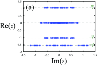
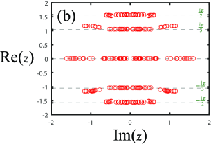
Figure 1: Patterns of $z$-roots (a) and $w$-roots (b) at any state with $N=8$ and $\eta=\frac{i\pi}{3}$.

From Fig.1 we observe the following $z$-roots patterns: (1) real $z_{j}^{(1)}$; (2) $-\frac{i\pi}{2}$ axis $z_{j}^{(2)}-\frac{i\pi}{2}$; (3) conjugate pair $z_{j}^{(3)}\pm\eta$. The corresponding $w$-roots patterns are: (1) real $w_{l}^{(1)}$; (2) $\pm\frac{i\pi}{2}$ axis $w_{l}^{(2)}\pm\frac{i\pi}{2}$; (3) conjugate pair $w_{l}^{(3)}\pm\eta$. Fig.2 below shows some relationship between the $w$-roots and the $z$-roots

$$\{w_{l}^{(2)}\}=\{z_{j}^{(3)}\},\qquad\{w_{l}^{(3)}\}=\{z_{j}^{(2)}\}.$$ (4.10)

These relations can be proven in the thermodynamic limit (the proof is relegated to Appendix B).

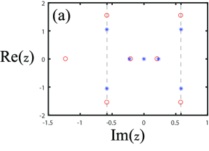
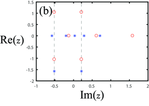
Figure 2: Comparing of $z$-roots and $w$-roots at the same state with $N=8$ and $\eta=\frac{i\pi}{3}$. The blue asterisks indicate $z$-roots and the red circles specify $w$-roots.

5 Thermodynamics at the point of $\eta=\frac{i\pi}{3}$

Based on the zero points BAEs (4.7-4.8) and the corresponding patterns of the $z$-roots and $w$-roots in the previous section, we in this section study the thermodynamics of the XXZ torus model at the point of $\eta=\frac{i\pi}{3}$.

5.1 Integral relations

In the thermodynamic limit $N\rightarrow\infty$, we define the densities of $z^{(l)}$-roots, $z^{(l)}$-holes, $w^{(l)}$-roots and $w^{(l)}$-holes per unit site as $\rho_{l}(z)$, $\rho_{l}^{h}(z)$, $\sigma_{l}(w)$ and $\sigma_{l}^{h}(w)$, respectively.

Setting $z_{j}=z_{j}^{(1)}$ and $z_{j}=z_{j}^{(3)}+\eta$ in BAEs (4.7), we obtain

$$\frac{\sinh^{N}(z_{j}^{(1)}+\frac{\eta}{2})\,\sinh^{N}(z_{j}^{(1)}-\frac{3\eta}{2})}{\sinh^{N}(z_{j}^{(1)}-\frac{\eta}{2})}=W_{0}\prod_{n=1}^{\bar{M}_{1}}\sinh(z_{j}^{(1)}-w_{n}^{(1)}-\frac{\eta}{2})$$

$$\times\prod_{k=1}^{M_{3}}\sinh(z_{j}^{(1)}-z_{k}^{(3)}+\eta)\sinh(z_{j}^{(1)}-z_{k}^{(3)}+\eta)\prod_{l=1}^{M_{2}}\sinh(z_{j}^{(1)}-z_{l}^{(2)}+\frac{\eta}{2})\sinh(z_{j}^{(1)}-z_{l}^{(2)}-\frac{3\eta}{2}),$$ (5.1)

$$\frac{\sinh^{N}(z_{j}^{(3)}+\frac{3\eta}{2})\,\sinh^{N}(z_{j}^{(3)}-\frac{\eta}{2})}{\sinh^{N}(z_{j}^{(3)}+\frac{\eta}{2})}=\,W_{0}\prod_{n=1}^{\bar{M}_{1}}\sinh(z_{j}^{(3)}-w_{n}^{(1)}+\frac{\eta}{2})$$

$$\times\prod_{k=1}^{M_{3}}\sinh(z_{j}^{(3)}-z_{k}^{(3)}-\eta)\sinh(z_{j}^{(3)}-z_{k}^{(3)}-\eta)\prod_{l=1}^{M_{2}}\sinh(z_{j}^{(3)}-z_{l}^{(2)}+\frac{3\eta}{2})\sinh(z_{j}^{(3)}-z_{l}^{(2)}-\frac{\eta}{2}),$$ (5.2)

respectively. In the above derivation, we have used the property $\sinh(u+i\pi)=-\sinh(u)$ and the relation (4.10). Dividing the complex conjugate of BAEs (5.1) (resp. BAEs (5.2)) by (5.1) (resp. (5.2)) and taking the logarithm of the resulting equations, we have

$$2\theta_{1}(z_{j}^{(1)}) = \frac{4\pi I_{j}^{(1)}}{N}-\frac{1}{N}\big{[}\sum_{n=1}^{\bar{M}_{1}}\theta_{1}(z_{j}^{(1)}-w_{n}^{(1)})$$ (5.3)

$$+\sum_{k=1}^{M_{3}}2\theta_{2}(z_{j}^{(1)}-z_{k}^{(3)})+\sum_{l=1}^{M_{2}}\theta_{1}(z_{j}^{(1)}-z_{l}^{(2)})\big{]},$$

$$2\theta_{1}(z_{j}^{(3)}) = \frac{4\pi I_{j}^{(3)}}{N}-\frac{1}{N}\big{[}\sum_{n=1}^{\bar{M}_{1}}\theta_{1}(z_{j}^{(3)}-w_{n}^{(1)})$$ (5.4)

$$+\sum_{k=1}^{M_{3}}2\theta_{2}(z_{j}^{(3)}-z_{k}^{(3)})+\sum_{l=1}^{M_{2}}\theta_{1}(z_{j}^{(3)}-z_{l}^{(2)})\big{]},$$

where $I_{j}^{(1)}$, $I_{j}^{(3)}$ denote the quantum numbers associated with the roots $z_{j}^{(1)}$, $z_{j}^{(3)}$, respectively, and $\theta_{n}(x)=2\cot^{-1}(\coth x\tanh\frac{n\gamma}{2})$. Furthermore, multiplying the complex conjugate of BAEs (5.1) (resp. BAEs (5.2)) by (5.1) (resp. (5.2)) and taking the logarithm of the resulting equations, we obtain

$$\ln |\sinh(z_{j}^{(1)}-\frac{3\eta}{2})|=\ln\,|W_{0}|+\frac{1}{N}\left[\sum_{n=1}^{\bar{M}_{1}}\ln|\sinh(z_{j}^{(1)}-w_{n}^{(1)}-\frac{\eta}{2})|\right.$$ (5.5)

$$\left.+\sum_{k=1}^{M_{3}}2\ln|(z_{j}^{(1)}-z_{k}^{(3)}+\eta)|+\sum_{l=1}^{M_{2}}\ln|\sinh(z_{j}^{(1)}-z_{l}^{(2)}+\frac{\eta}{2})\sinh(z_{j}^{(1)}-z_{l}^{(2)}-\frac{3\eta}{2})|\right],$$

$$\ln |\sinh(z_{j}^{(3)}+\frac{3\eta}{2})|=\ln\,|W_{0}|+\frac{1}{N}\left[\sum_{n=1}^{\bar{M}_{1}}\ln|\sinh(z_{j}^{(3)}-w_{n}^{(1)}+\frac{\eta}{2})|\right.$$ (5.6)

$$\left.+\sum_{k=1}^{M_{3}}2\ln|(z_{j}^{(3)}-z_{k}^{(3)}-\eta)|+\sum_{l=1}^{M_{2}}\ln|\sinh(z_{j}^{(3)}-z_{l}^{(2)}-\frac{\eta}{2})\sinh(z_{j}^{(3)}-z_{l}^{(2)}+\frac{3\eta}{2})|\right].$$

Taking the continuum limits and derivatives of Eqs.(5.3)-(5.6), we have

$$2a_{1}(z) = 2\rho_{1}(z)+2\rho_{1}^{h}(z)-a_{1}*\sigma_{1}(z)+2a_{2}*\rho_{3}(z)+a_{1}*\rho_{2}(z),$$ (5.7)

$$b_{3}(z) = b_{1}*\sigma_{1}(z)+2b_{2}*\rho_{3}(z)+(b_{1}+b_{3})*\rho_{2}(z),$$ (5.8)

$$2a_{1}(z) = 2\rho_{3}(z)+2\rho_{3}^{h}(z)-a_{1}*\sigma_{1}(z)+2a_{2}*\rho_{3}(z)+a_{1}*\rho_{2}(z),$$ (5.9)

$$b_{3}(z) = b_{1}*\sigma_{1}(z)+2b_{2}*\rho_{3}(z)+(b_{1}+b_{3})*\rho_{2}(z),$$ (5.10)

where $a_{n}(z)=\sin(n\gamma)/[\pi(\cosh 2z-\cos n\gamma)]$, $b_{n}(z)=\sinh(2z)/[\pi(\cosh 2z-\cos n\gamma)]$ and the symbol $*$ indicates convolution.

For the $z$-roots pattern (2) $z_{j}=z_{j}^{(2)}-\frac{i\pi}{2}$, the BAEs (4.7) can be rewritten as

$$\frac{\sinh^{N}(z_{j}^{(2)}-\eta)\,\sinh^{N}(z_{j}^{(2)})}{\sinh^{N}(z_{j}^{(2)}+\eta)}=\,W_{0}\prod_{n=1}^{\bar{M}_{1}}\sinh(z_{j}^{(2)}-w_{n}^{(1)}+\eta)$$

$$\hskip 5.69046pt\times\prod_{k=1}^{M_{3}}\sinh(z_{j}^{(2)}-z_{k}^{(3)}-\frac{\eta}{2})\sinh(z_{j}^{(2)}-z_{k}^{(3)}-\frac{\eta}{2})\prod_{l=1}^{M_{2}}\sinh(z_{j}^{(2)}-z_{l}^{(2)}-\eta)\sinh(z_{j}^{(2)}-z_{l}^{(2)}).$$ (5.11)

Due to the existence of the infinitesimal term $\prod_{l}\sinh(z_{j}^{(2)}-z_{l}^{(2)})$, we can only divide the complex conjugate of BAEs (5.11) by (5.11) to eliminate the infinitesimal term. Taking the logarithm of the resulting equations, we obtain

$$2\theta_{2}(z_{j}^{(2)})= \frac{4\pi I_{j}^{(2)}}{N}-\frac{1}{N}\big{[}\sum_{n=1}^{\bar{M}_{1}}\theta_{2}(z_{j}^{(2)}-w_{n}^{(1)})$$ (5.12)

$$+\sum_{k=1}^{M_{3}}2\theta_{1}(z_{j}^{(2)}-z_{k}^{(3)})+\sum_{l=1}^{M_{2}}\theta_{2}(z_{j}^{(2)}-z_{l}^{(2)})\big{]},$$

where $I_{j}^{(2)}$ denote the quantum numbers associated with the roots $z_{j}^{(2)}$. Similarly, taking the derivative of Eq.(5.12) we have

$$2a_{2}(z) = \rho_{2}(z)+\rho_{2}^{h}(z)-a_{2}*\sigma_{1}(z)+2a_{1}*\rho_{3}(z)+a_{2}*\rho_{2}(z).$$ (5.13)

To determine the thermodynamics, we also need to obtain the density $\sigma_{1}(w)$. Setting $w_{j}=w_{j}^{(1)}$ in BAEs (4.8), we obtain

$$\sinh^{N}(w_{j}^{(1)}+\eta)\sinh^{N}(w_{j}^{(1)}-\eta)=\Lambda^{2}_{0}\prod_{n=1}^{M_{1}}\sinh(w_{j}^{(1)}-z_{n}^{(1)}+\frac{\eta}{2})\sinh(w_{j}^{(1)}-z_{n}^{(1)}-\frac{\eta}{2})$$

$$\hskip 2.84544pt\times\prod_{k=1}^{M_{3}}\sinh(w_{j}^{(1)}-z_{k}^{(3)}+\frac{3\eta}{2})\sinh(w_{j}^{(1)}-z_{k}^{(3)}+\frac{\eta}{2})\sinh(w_{j}^{(1)}-z_{k}^{(3)}-\frac{\eta}{2})\sinh(w_{j}^{(1)}-z_{k}^{(3)}+\frac{3\eta}{2})$$

$$\hskip 2.84544pt\times\prod_{l=1}^{M_{2}}\sinh(w_{j}^{(1)}-z_{l}^{(2)}-\eta)\sinh(w_{j}^{(1)}-z_{l}^{(2)}+\eta).$$ (5.14)

Taking the logarithm and derivative of this equation, we have

$$b_{2}(z) = b_{1}*\rho_{1}(z)+(b_{1}+b_{3})*\rho_{3}(z)+b_{2}*\rho_{2}(z).$$ (5.15)

In addition, the expressions (4.3)-(4.4) show that the total number of $z$-roots and $w$-roots must be $N-1$ and $N$ respectively, i.e.,

$$N\int_{-\infty}^{+\infty}[\rho_{1}(z)+\rho_{2}(z)+2\rho_{3}(z)]dz=N-1,$$ (5.16)

$$N\int_{-\infty}^{+\infty}[\sigma_{1}(z)+2\rho_{2}(z)+2\rho_{3}(z)]dz=N.$$ (5.17)

Now combining (5.7)-(5.10) and (5.15)-(5.17), we obtain

$$\sigma_{1}(z)=2g*[\rho_{1}(z)+\frac{1}{2N}(\delta(-\infty)+\delta(+\infty))]-\rho_{2}(z),$$ (5.18)

$$\rho_{3}^{h}(z)=\rho_{1}(z)+\frac{1}{2N}[\delta(-\infty)+\delta(+\infty)],$$ (5.19)

$$\rho_{1}^{h}(z)=\rho_{3}(z)+\frac{1}{2N}[\delta(-\infty)+\delta(+\infty)],$$ (5.20)

where $g(z)=1/(2\gamma\cosh(3z))$. The existence of $\frac{1}{2N}(\delta(-\infty)+\delta(+\infty))$ is in order to satisfy the constraints (5.16) and (5.17). Using the relations (5.18)-(5.20), after some calculations, we can rewrite (5.7) and (5.13) as

$$\rho_{1}(z)+\rho_{3}(z) = a_{1}(z)+a_{2}*\rho_{1}(z)-a_{2}*\rho_{3}(z)-a_{1}*\rho_{2}(z)$$ (5.21)

$$+a_{2}*\frac{1}{2N}(\delta(-\infty)+\delta(+\infty))-\frac{1}{2N}(\delta(-\infty)+\delta(+\infty)),$$

$$\rho_{2}(z)+\rho_{2}^{h}(z) = 2g*[\rho_{1}(z)+\frac{1}{2N}(\delta(-\infty)+\delta(+\infty))].$$ (5.22)

Applying the Fourier transform and the inverse Fourier transform, we can express the densities $\rho_{3}(z)$ and $\rho_{2}^{h}(z)$ in terms of the densities $\rho_{1}(z)$ and $\rho_{2}(z)$ as follows

$$\rho_{3}(z) = g(z)+2g*g*[\rho_{1}(z)+\frac{1}{2N}(\delta(-\infty)+\delta(+\infty))]-\rho_{1}(z)$$ (5.24)

$$-\frac{1}{2N}(\delta(-\infty)+\delta(+\infty))-g*\rho_{2}(z)$$

$$\rho_{2}^{h}(z) = 2g*[\rho_{1}(z)+\frac{1}{2N}(\delta(-\infty)+\delta(+\infty))]-\rho_{2}(z).$$ (5.25)

5.2 NLIEs and free eneegy

Thanks to the relations (5.19) and (5.20) of the densities $\rho_{1}(z)$ and $\rho_{3}(z)$, the number of the possible physical states in an infinitely small interval $[z,z+dz]$ of the $z$ space is given by

$$d\Omega(z)=\sum_{l=2}^{3}\frac{[N(\rho_{l}(z)+\rho_{l}^{h}(z))dz]!}{[N(\rho_{l}(z))dz]![N(\rho_{l}^{h}(z))dz]!}.$$ (5.26)

With the help of Sterling’s formula $\ln N!\approx N\ln N$, we obtain the entropy in the interval

$$dS(z) =\ln d\Omega(z)$$ (5.27)

$$\approx\sum_{l=2}^{3}N{\{[\rho_{l}(z)+\rho_{l}^{h}(z)]ln[\rho_{l}(z)+\rho_{l}^{h}(z)]}-\rho_{l}(z)ln\rho_{l}(z)-\rho_{l}(z)ln\rho_{l}^{h}(z)]\}dz.$$

We define the relative density of the free energy as

$$f=\frac{F}{N}=\frac{E-TS}{N}=e-Ts.$$ (5.28)

Using the energy expression (4.9) and combining the $z$-roots patterns, the energy density is given by

$$e=\sqrt{3}\pi\int_{-\infty}^{+\infty}[a_{1}(z)\rho_{1}(z)-a_{2}(z)\rho_{2}(z)-a_{1}(z)\rho_{3}(z)]dz-\cosh(\eta).$$ (5.29)

Substituting (5.27) and (5.29) into (5.28), we have

$$f = \sqrt{3}\pi\int_{-\infty}^{+\infty}[a_{1}(z)\rho_{1}(z)-a_{2}(z)\rho_{2}(z)-a_{1}(z)\rho_{3}(z)]dz-\cosh(\eta)$$ (5.30)

$$-T\sum_{i=2}^{3}\int_{-\infty}^{+\infty}{\{[\rho_{i}(z)+\rho_{i}^{h}(z)]ln[\rho_{i}(z)+\rho_{i}^{h}(z)]}-\rho_{i}(z)ln\rho_{i}(z)-\rho_{i}(z)ln\rho_{i}^{h}(z)]\}dz.$$

For a thermal equilibrium state, the free energy should be minimized with respect to variations of $\rho_{1}(z)$ and $\rho_{2}(z)$ respectively, namely,

$$\frac{\delta f}{\delta\rho_{1}(z)}=0,\,\,\,\qquad\frac{\delta f}{\delta\rho_{2}(z)}=0.$$ (5.31)

Substituting (5.24), (5.25) and (5.30) into (5.31), and using $a_{2}(z)=a_{1}*g(z)$, we obtain

$$2\sqrt{3}\pi g(z)-T\{2g*g*\ln(1+\eta_{3}(z))+\ln(\eta_{3}^{-1}(z))+2g*\ln(1+\eta^{-1}_{2}(z))\}=0,$$ (5.32)

$$\ln(\eta_{2}(z))-g*\ln(1+\eta_{3}(z))=0,$$ (5.33)

where

$$\eta_{l}(z)=\frac{\rho_{l}^{h}(z)}{\rho_{l}(z)},\qquad l=2,3.$$ (5.34)

Putting (5.33) in (5.32) and combining with (5.18), we can reduce (5.32) and (5.33) to

$$\ln(\eta_{3}(z))=-\frac{2\sqrt{3}\pi g(z)}{T}+2g*\ln(1+\eta_{2}(z)),$$ (5.35)

$$\ln(\eta_{2}(z))=g*\ln(1+\eta_{3}(z)).$$ (5.36)

Thus $\eta_{2}(z)$ and $\eta_{3}(z)$ can be determined by iteration. Substituting (5.35) and (5.36) into (5.30), we obtain the free energy of XXZ torus model described by the Hamiltonian (2.1)-(2.2) with $\eta=\frac{i\pi}{3}$ as

$$f=e_{g}-T\int_{-\infty}^{+\infty}{g(z)ln(1+\eta_{3}(z))}dz,$$ (5.37)

where $e_{g}=-\sqrt{3}\pi\int_{-\infty}^{+\infty}a_{1}(z)g(z)dz-\cosh(\eta)$ is the ground state energy density. The free energy vs the temperature $T$ is shown in Fig.3. Based on the obtained free energy, other thermodynamic quantities such as specific heat can be calculated directly.

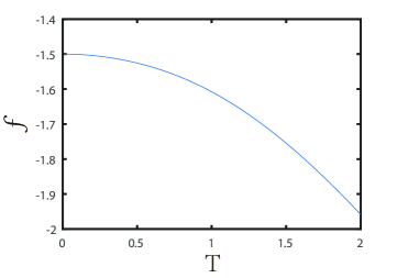
Figure 3: Free energy $f$ vs Temperature for the anti-periodic XXZ chain.

6 Conclusions

In this paper, we have studied the thermodynamics of the antiperiodic XXZ spin chain with the anisotropic parameter $\eta=\frac{i\pi}{3}$ at finite temperature. We obtain the $t-W$ relations of the transfer matrix and the corresponding eigenvalues. We parameterize the eigenvalues of the transfer matrix and the fused transfer matrix by their zero points instead of Bethe roots. By substituting the zero points into the $t-W$ relation, the homogeneous zero points BAEs are obtained. The patterns of distribution of the zero points at $\eta=\frac{i\pi}{3}$ are determined by solving the BAEs. Based on these results, we have defined the densities of different zero points patterns and reconstructed entropy. Finally, we obtain the NLIEs and free energy describing the thermodynamics of the XXZ torus model with the anisotropy parameter $\eta=\frac{i\pi}{3}$. Our results indicate that the twisted boundary has not effect on the free energy at the point of $\eta=\frac{i\pi}{3}$ in the thermodynamic limit.

Appendix A Proof of the $t-W$ relation

In this appendix we prove the operator relation (3.2) between the transfer matrices by using the fusion technique [31, 32].

For this purpose, let us introduce the (anti)symmetric subspaces $W^{(\pm)}$ of $\mathbb{C}^{2}\otimes\mathbb{C}^{2}$, defined by $W^{(\pm)}=P^{(\pm)}_{12}(\mathbb{C}^{2}\otimes\mathbb{C}^{2})$. Let $\{|i\rangle|i=1,2\}$ be an orthnormal basis of $\mathbb{C}^{2}$. It is easy to see that $W^{(+)}$ is a $3$-dimensional subspace spanned by the orthnormal basis $\{|11\rangle,\,\frac{1}{\sqrt{2}}(|12\rangle+|21\rangle),\,|22\rangle\}$, while $W^{(-)}$ is an $1$-dimensional subspace spanned by $\{\frac{1}{\sqrt{2}}(|12\rangle-|21\rangle)\}$. The QYBE (2.8) and the fusion condition (2.13) allow us to derive the relation

$$R_{23}(u)R_{13}(u-\eta)P^{(-)}_{12}=P^{(-)}_{12}R_{23}(u)R_{13}(u-\eta)P^{(-)}_{12}=\frac{\sinh(u+\eta)\sinh(u-\eta)}{\sinh\eta\sinh\eta}\times{\rm id}.$$ (A.1)

Direct calculation shows that

$$P^{(+)}_{12}\,R_{23}(u)\,R_{13}(u-\eta)\,P^{(+)}_{12}=\frac{\sinh u}{\sinh\eta}\,R^{(1,\frac{1}{2})}_{\{12\}\,3}(u),$$ (A.2)

where the fused $R$-matrix $R^{(1,\frac{1}{2})}_{\{12\}\,3}(u)$, in the the basis $\{|11\rangle,\,\frac{1}{\sqrt{2}}(|12\rangle+|21\rangle),\,|22\rangle\}$, is given by

$$R^{(1,\frac{1}{2})}_{\{12\}\,3}(u)=\left(\begin{array}[]{cccccc}\frac{\sinh(u+\eta)}{\sinh\eta}&&&&&\\[6.0pt] &\frac{\sinh(u-\eta)}{\sinh\eta}&\sqrt{2}&&&\\[6.0pt] &\sqrt{2}\cosh\eta&\frac{\sinh u}{\sinh\eta}&&&\\[6.0pt] &&&\frac{\sinh u}{\sinh\eta}&\sqrt{2}\cosh\eta&\\[6.0pt] &&&\sqrt{2}&\frac{\sinh(u-\eta)}{\sinh\eta}&\\[6.0pt] &&&&&\frac{\sinh(u+\eta)}{\sinh\eta}\end{array}\right).$$ (A.9)

The relation (A.1) leads to

$$P^{(-)}_{12}\sigma^{x}_{1}\sigma^{x}_{2}T_{2}(u)\,T_{1}(u-\eta)P^{(-)}_{12}=-a(u)\,d(u-\eta)\times{\rm id}.$$ (A.10)

Moreover, the relations (A.1) and (A.2) allow us to express the second term of the equation (3.1) in terms of the fused monodromy matrix as

$$P^{(+)}_{12}\sigma^{x}_{1}\sigma^{x}_{2}T_{2}(u)\,T_{1}(u-\eta)P^{(+)}_{12}=\prod_{l=1}^{N}\frac{\sinh(u-\theta_{l})}{\sinh\eta}\sigma_{\{12\}}^{x}\,T^{(1,\frac{1}{2})}_{\{12\}}(u),$$ (A.11)

where the fused Pauli matrix is defined as

$$\sigma_{\{12\}}^{x}=\left(\begin{array}[]{ccc}0&0&1\\ 0&1&0\\ 1&0&0\\ \end{array}\right),$$ (A.15)

and the fused monodromy matrix $T^{(1,\frac{1}{2})}_{\{12\}}(u)$ can be expressed in terms of the fused $R$-matrix $R^{(1,\frac{1}{2})}_{\{12\}\,3}(u)$ given by (A.2)

$$T^{(1,\frac{1}{2})}_{\{12\}}(u)=R^{(1,\frac{1}{2})}_{\{12\}\,N}(u-\theta_{N})\cdots R^{(1,\frac{1}{2})}_{\{12\}\,1}(u-\theta_{1}).$$ (A.16)

Then the fused transfer matrix $\mathbb{W}(u)$ is given by the trace over the subspace $W^{(+)}$ of the fused monodromy matrix $T^{(1,\frac{1}{2})}_{\{12\}}(u)$ and $\sigma^{x}_{\{12\}}$

$$\mathbb{W}(u)=tr\left\{\sigma_{\{12\}}^{x}T^{(1,\frac{1}{2})}_{\{12\}}(u)\right\}.$$ (A.17)

From the construction of (A.9) and (A.16), we know that the matrix elements of the fused monodromy matrix $T^{(1,\frac{1}{2})}_{\{12\}}(u)$ and $\sigma^{x}_{\{12\}}$, as a function of $u$, are operator-valued trigonometric polynomials of degrees up to $N$. This completes the proof of the $t-W$ relation (3.2).

Appendix B Proof of the relation between $z$-roots and $w$-roots

In this appendix we prove the relations (4.10) by using the $t-W$ relation (4.2). Setting $u=z_{j}-\frac{\eta}{2}$ and $u=z_{j}+\frac{\eta}{2}$ in (4.2), respectively, we obtain

$$\frac{\sinh^{N}(z_{j}+\frac{\eta}{2})\,\sinh^{N}(z_{j}-\frac{3\eta}{2})}{\sinh^{N}\eta\,\sinh^{N}\eta}=\frac{\sinh^{N}(z_{j}-\frac{\eta}{2})}{\sinh^{N}\eta}\,W_{0}\prod_{l=1}^{N}\frac{\sinh(z_{j}-w_{l}-\frac{\eta}{2})}{\sinh\eta},$$ (B.1)

$$\frac{\sinh^{N}(z_{j}+\frac{3\eta}{2})\,\sinh^{N}(z_{j}-\frac{\eta}{2})}{\sinh^{N}\eta\,\sinh^{N}\eta}=\frac{\sinh^{N}((z_{j}+\frac{\eta}{2})}{\sinh^{N}\eta}\,W_{0}\prod_{l=1}^{N}\frac{\sinh(z_{j}-w_{l}+\frac{\eta}{2})}{\sinh\eta}.$$ (B.2)

Dividing (B.2) by (B.1), we have

$$\frac{\sinh^{2N}(z_{j}-\frac{\eta}{2})}{\sinh^{2N}(z_{j}+\frac{\eta}{2})}=\prod_{l=1}^{N}\frac{\sinh(z_{j}-w_{l}+\frac{\eta}{2})}{\sinh(z_{j}-w_{l}-\frac{\eta}{2})}.$$ (B.3)

For complex $z$-roots $z_{j}$ with negative imaginary part and ${\rm Im}(z_{j})>-\frac{\pi}{2}$, we readily have

$$\Big{|}\sinh(z_{j}-\frac{\eta}{2})\Big{|}>\Big{|}\sinh(z_{j}+\frac{\eta}{2})\Big{|}.$$ (B.4)

This indicates that the module of the left hand side of (B.3) is bigger than 1. Thus in the thermodynamic limit $N\rightarrow\infty$, the left hand side tends to infinity exponentially. To keep (B.3) holding, the right hand side of (B.3) must also approach infinity in the same order. Thus the denominator of the first term in the right hand side must tend to zero exponentially, which leads to $z_{j}-w_{l}-\frac{\eta}{2}\rightarrow 0$. Similarly, we can obtain $z_{j}-w_{l}+\frac{\eta}{2}\rightarrow 0$ for complex $z$-roots $z_{j}$ with positive imaginary part. Therefore, for the $z$-roots patterns (3) conjugate pair $z_{j}^{(3)}\pm\eta$, the $w$-root structure satisfies $w_{l}=z_{j}^{(3)}\pm\frac{i\pi}{2}=w_{j}^{(2)}\pm\frac{i\pi}{2}$.

Next, we consider the $z$-roots patterns (2) $-\frac{i\pi}{2}$ axis $z_{j}^{(2)}-\frac{i\pi}{2}$. Putting $z_{j}=z_{j}^{(2)}-\frac{i\pi}{2}$ in (B.1), we have

$$\frac{\sinh^{N}(z_{j}-\eta)\,\sinh^{N}(z_{j})}{\sinh^{N}(z_{j}+\eta)}=\,W_{0}\prod_{l=1}^{N}\sinh(z_{j}-w_{l}+\eta).$$ (B.5)

Multiplying the complex conjugate of BAEs (B.5) by (B.5) and taking the logarithm of the resulting equation, we obtain

$$2N\ln|\sinh(z_{j}^{(2)})|=2\ln|W_{0}|+\prod_{l=1}^{N}\ln|\sinh(z_{j}^{(2)}-w_{l}+\eta)\sinh(z_{j}^{(2)}-w_{l}^{*}-\eta)|.$$ (B.6)

When we take the continuum limit of (B.6) in the thermodynamic limit, the left hand side of (B.6) will contribute a $\delta$-function. To keep (B.6) holding, the antilogarithm of the second term in the right hand side must tend to zero exponentially, which leads to $z_{j}^{(2)}-w_{l}+\eta\rightarrow 0$ and $z_{j}^{(2)}-w_{l}^{*}-\eta\rightarrow 0$. Therefore, for the $z$-roots pattern (2) $\frac{i\pi}{2}$ axis $z_{j}^{(2)}-\frac{i\pi}{2}$, the $w$-root structure satisfies $w_{j}=z_{j}^{(2)}\pm\eta=w_{j}^{(3)}\pm\eta$. As a result, the relation (4.10) is achieved. This completes our proof.

References

- [1] C.M. Yung, M.T. Batchelor, Nucl. Phys. B 446 (1995) 461.
- [2] M.T. Batchelor, R.J. Baxter, M.J. O’Rourke, C.M. Yung, J. Phys. A 28 (1995) 2759.
- [3] W. Galleas, Nucl. Phys. B 790 (2008) 524.
- [4] S. Niekamp, T. Wirth, H. Frahm, J. Phys. A 42 (2009) 195008.
- [5] H. Frahm, J.H. Grelik, A. Seel, T. Wirth, J. Phys. A 44 (2011) 015001.
- [6] G. Niccoli, Nucl. Phys. B 870 (2013) 397.
- [7] M. Vanicat, Nucl. Phys. B 929 (2018) 298.
- [8] R. Frassek, C. Giardina, J. Kurchan, SciPost Phys. 9 (2020) 054.
- [9] Z. Chen, J. de Gier, M. Wheeler, Int. Math. Res. Not. 19 (2020) 5872.
- [10] U. Godreau and S. Prolhac, J. Phys. A 53 (2020) 385006.
- [11] N. Andrei et al., J. Phys. A 53 (2020) 453002.
- [12] A. Bastianello, L. Piroli, P. Calabrese, Phys. Rev. Lett. 120 (2018) 190601.
- [13] M. Mestyán, B. Bertini, L. Piroli, et al., Phys. Rev. B 99 (2019) 014305.
- [14] A. Fontanella, A. Torrielli, J. High Energy Phys. 09 (2017) 1.
- [15] Y. Jiang, S. Komatsu, E. Vescovi, J. High Energy Phys. 07 (2020) 1.
- [16] M. De Leeuw, C. Paletta, A. Pribytok, et al., J. High Energy Phys. 02 (2021) 1.
- [17] H. Bethe, Z. Phys. 71 (1931) 205.
- [18] M. Gaudin, The Bethe Wavefunction, Cambridge University Press, London, 2014.
- [19] E.K. Sklyanin, L.D. Faddeev, Sov. Phys. Dokl. 23 (1978) 902.
- [20] L.A. Takhtadzhan, L.D. Faddeev, Russ. Math. Surv. 34 (1979) 11.
- [21] V.E. Korepin, N.M. Boliubov, A.G. Izergin, Quantum Inverse Scattering Method and Correlation Functions, Cambridge University Press, London, 1993.
- [22] J. Cao, W.-L. Yang, K. Shi, Y. Wang, Phys. Rev. Lett. 111 (2013) 137201.
- [23] Y. Wang, W.-L. Yang, J. Cao, K. Shi, Off-Diagonal Bethe Ansatz for Exactly Solvable Models, Springer-Verlag, Berlin Heidelberg, 2015.
- [24] X. Zhang, Y.-Y. Li, J. Cao, W.-L. Yang, K. Shi, Y. Wang, Nucl. Phys. B 893 (2015) 70.
- [25] X. Zhang, Y.-Y. Li, J. Cao, W.-L. Yang, K. Shi, Y. Wang, J. Stat. Mech. (2015) P05014.
- [26] M. Gaudin, Phys. Rev. Lett. 26 (1971) 1301.
- [27] M. Takahashi, Prog. Theor. Phys. 46 (1971) 401.
- [28] M. Takahashi, Thermodynamics of One-Dimensional Solvable Models, Cambridge University Press, London, 2005.
- [29] Y. Qiao, P. Sun, J. Cao, W.-L. Yang, K. Shi, Y. Wang, Phys. Rev. B 102 (2020) 085115.
- [30] Y. Qiao, J. Cao, W.-L. Yang, K. Shi, Y. Wang, Phys. Rev. B 103 (2021) L220401.
- [31] P.P. Kulish, N. Yu. Reshetikhin, E.K. Sklyanin, Lett. Math. Phys. 5 (1981) 393.
- [32] A.N. Kirillov, N.Yu. Reshetikhin, J. Sov. Math. 35 (1986) 2627.