Non-linear population discrete models with two time scales: re-scaling of part of the slow process

Abstract

In this work we present a reduction result for discrete time systems with two time scales. In order to be valid, previous results in the field require some strong hypotheses that are difficult to check in practical applications. Roughly speaking, the iterates of a map as well as their differentials must converge uniformly on compact sets. Here, we eliminate the hypothesis of uniform convergence of the differentials at no significant cost in the conclusions of the result. This new result is then used to extend to nonlinear cases the reduction of some population discrete models involving processes acting at different time scales. In practical cases, some processes that occur at a fast time scale are often only measured at slow time intervals, notably mortality. For a general class of linear models that include such kind of processes, it has been shown that a more realistic approach requires the re-scaling of those processes to be considered at the fast time scale. We develop the same type of re-scaling in some nonlinear models and prove the corresponding reduction results. We also provide an application to a particular model of a structured population in a two-patch environment.

keywords:discrete-time system, time scales, re-scaling, structured population.

1 Introduction

We consider discrete systems in the framework of population dynamics models. The complexity of these models can be treated distinguishing the different time scales at which the different processes involved act. In an idealization of this approach we proposed (see Bravo de la Parra et al. (2013) and references therein) to merge two different processes acting at different time scales in a single model as we describe next. The effect of the fast process during a fast time unit is represented by a general map $F$, and a general map $S$ describes the slow process in a slow time unit. We choose this latter as the time unit of the common discrete model. If the slow time unit is approximately $k$ times larger than the fast one, we consider that during this interval the fast process acts sequentially $k$ times followed by the slow process acting once. The combined effect of both processes during a slow time unit is therefore represented by the composition of map $S$ and the k-th iterate $F^{(k)}$ of map $F$. If we let vector $X(t)$ represent the population state at time $t$, the general form of the system is:

$$X(t+1)=S\left(F^{(k)}\left(X(t)\rule{0.0pt}{8.61108pt}\right)\right)$$ (1)

The subsequent issue is to take advantage of the existence of time scales to reduce the proposed system. The reduction we are referring to can be considered to be part of the so-called methods of aggregation of variables, that exist in different mathematical settings Auger et al. (2008a, b). It consists on finding a certain number of global variables, which are functions of the state variables, and a reduced system, approximately describing their dynamics, such that it is possible to get information on the asymptotic behaviour of the solutions of the original system in terms of this reduced system. This procedure has a direct interpretation in terms of ecological hierarchy theory Auger and Lett (2003) and the concept of up-scaling through ecological hierarchical levels Lischke et al. (2007); Levin (1992). In general, aggregation methods are approximate in the sense that quantitatively the dynamics of the original system can not be described exactly by the dynamics of the reduced one. However, the error incurred decreases when the ratio of time scales increases and, for a large enough value of this ratio, the two systems have the same qualitative dynamics.

In Sanz et al. (2008) it is proved that system (1) can be reduced if the limit of the iterates of map $F$ exists and can be expressed as the composition of two maps going through a lower dimensional space. With additional hypotheses it is possible to extract information on the asymptotic behaviour of the solutions of system (1) by means of the reduced system. To be specific, one can study the existence, stability and basins of attraction of steady states and periodic solutions of the original system by performing the study for the corresponding aggregated system. The additional hypotheses essentially consist in the convergence on compact sets of the $F$ iterates and their differentials. However, this latter assumption is generally too involved, if not impossible, to be proved in particular applications.

The main result in this work proves that the mere convergence on compact sets of the $F$ iterates is enough to obtain almost the same results as in Sanz et al. (2008). The downside is that we cannot guarantee the convergence of the system dynamics to the attractor, equilibrium or periodic solution, obtained through the analysis of the reduced system. However, we prove that this dynamics remains as close to the attractor as desired if the ratio of time scales is sufficiently large. Therefore, from the point of view of population dynamics models this last property is good enough to obtain valuable qualitative results.

This reduction result is applied in the context of discrete-time models of structured metapopulations with two time scales. The aim is to extend to the nonlinear case certain results obtained in Nguyen-Huu et al. (2011) for linear models. In structured metapopulation models that distinguish time scales, biological evidence suggest associating the slow one to the local demography (maturation, survival, reproduction) and the fast one to the movements between patches. When we express this in the form of system (1) we are representing that individuals perform at first a series of $k$ dispersal events between patches followed by a demographic event in the arrival patch. This way of separating slow and fast processes seems acceptable as far as reproduction is concerned, particularly in the case of populations with non-overlapping generations. Nevertheless, it is arguable whether survival should be considered at the slow time scale because deaths may occur at any moment of a slow time interval, i.e., in any of the patches through which individuals pass during this interval. In order to include this issue in the model, and having in mind that survival data may only exist for slow time units, in Nguyen-Huu et al. (2011) it is proposed to move survival from the slow to the fast process by approximating its effect during the fast time unit, i.e., re-scaling survival to the fast time scale.

According to this discussion, we present two general discrete-time models of structured metapopulations with two time scales. In the first one we consider the effect of survival in the time step corresponding to the slow process and, in the second one, in that corresponding to the fast process. The main result of this work makes it possible to extend the reduction method to the latter case.

This general framework is used to illustrate the effects of fast dispersals on local demography that emerge at the global metapopulation level. To this end, we extend the non-spatial model presented in Veprauskas and Cushing (2017) to a habitat with two patches between which fast dispersals are considered. The model is structured into three classes: juveniles and two adult stages. Adults that reproduce at the end of an interval of time do not reproduce at the end of the following one. A fraction of those not having reproduced do so at the end of the following interval. Thus, adults are classified into those reproducing at the end of the time interval, active adults, and those who do not, inactive adults. The aim of this consideration is studying the reproductive synchrony of adults. The model in Veprauskas and Cushing (2017) is a discrete time nonlinear matrix model whose inherent projection matrix is imprimitive Cushing (2015). This entails that the stability of the extinction equilibrium when $R_{0}$ increases through 1 bifurcates either to the stability of a non-extinction equilibrium or of a synchronous 2-cycle. The first option represents adults reproductive asynchrony whereas the second one is associated to reproductive synchrony.

Both metapopulation models, with or without re-scaled survival, and with local dynamics based on the model Veprauskas and Cushing (2017), can be studied through their associated reduced systems. Indeed, these have the same functional form as the system in Veprauskas and Cushing (2017) so that the results therein can be applied.

The main result on systems reduction is developed in Section 2. Two general discrete-time models of structured metapopulations with two time scales are presented in Section 3. The first one considers the dispersal process to be fast and the local demographic one, including survival, to be slow, whilst in the second one survival is transferred from the slow to the fast process. These two general models are applied in Section 4 to the particular case of a population structured into three classes inhabiting in a two-patch environment. With the help of these two particular models we illustrate how the effect of fast dispersals can make emerge at the global level asymptotic properties different from those occurring at the local level. The models are also used to show that the modelling choice regarding survival can imply drastic changes in behavior. A discussion and an appendix with the proofs of some results complete the work.

2 Reduction of slow-fast discrete systems

The point of departure is the paper Sanz et al. (2008) so we recall the presentation therein.

Let $N\in\mathbb{Z}_{+}\$and let $\Omega_{N}\subset\mathbb{R}^{N}$ be a set with non-empty interior. We start by introducing the original or complete model in the following general form:

$$X_{k}(t+1)=H_{k}\left(X_{k}(t)\right)$$ (2)

where $k\in\mathbb{Z}_{+}$ and $H_{k}:\Omega_{N}\longrightarrow\Omega_{N},\ H_{k}\in\mathcal{C}^{1}(\Omega_{N})$. System (1) is a particular case of system (2) where $H_{k}=S\circ F^{(k)}$.

In order to carry out the reduction of the model, we assume the following conditions:

Hypothesis 1.

The following pointwise limit exists in $\Omega_{N}$

$$\lim_{k\rightarrow\infty}H_{k}(X)=:H(X)\in\mathcal{C}^{1}(\Omega_{N}).$$ (3)

Hypothesis 2.

There exist a subset $\Omega_{q}\subset\mathbb{R}^{q}$ with $q<N$ and two maps
$G:\Omega_{N}\rightarrow\Omega_{q}$ and $T:\Omega_{q}\rightarrow\Omega_{N}$ of class $\mathcal{C}^{1}$ on their respective domains such that

$$H=T\circ G.$$ (4)

The approximate reduction of system (2) is carried out in two steps. First, we define the auxiliary system

$$X(t+1)=H(X(t)).$$ (5)

Applying $G$ to both members of the previous expression we have

$$G(X(t+1))=G\circ H(X(t))=G\circ T\circ G(X(t)),$$

and so by defining the global variables

$$Y(t):=G(X(t))\in\mathbb{R}^{q},$$ (6)

we obtain the reduced or aggregated system

$$Y(t+1)=\bar{H}(Y(t)),$$ (7)

where we have introduced the notation $\bar{H}:=G\circ T$.

Note that through this procedure we have constructed an approximation that allows us to reduce a system with $N$ variables to a new system with $q$ variables. In most practical applications, $q$ is much smaller than $N$.

The work Sanz et al. (2008) presents results that allow one to relate the existence of equilibrium points and periodic orbits for systems (2) and (7). More specifically, if certain conditions are met (see below) and the aggregated system has a hyperbolic $p$-periodic point $Y^{\ast}$ ($p\in\mathbb{N}$), then for a large enough value of $k$ the original system has a hyperbolic associated $p$-periodic point $X_{k}^{\ast}$ that can be approximated in terms of $Y^{\ast}$. Moreover, $X_{k}^{\ast}$ is (locally) asymptotically stable (resp. unstable) if and only if $Y^{\ast}$ is (locally) asymptotically stable (resp. unstable) and, in the first case, the basin of attraction of $X_{k}^{\ast}$ can be approximated in terms of that corresponding to $Y^{\ast}$.

For the previous results to hold, in addition to Hypotheses 1 and 2 one must include two additional conditions. The first one is:

Hypothesis 3.

The limit in (3) is uniform on all compact sets of $\Omega_{N}$.

The second condition is that $\lim_{k\rightarrow\infty}DH_{k}=DH$ uniformly on compact sets of $\Omega_{N}$, where $DH$ denotes the differential.

In practice, when applying approximate reduction techniques to population models even in simple settings, the (uniform) convergence of the differentials required in the second condition is difficult to check and involves lengthy reasonings and calculations (see for example the proofs in Marvá et al. (2013, 2009)). In more general situations, proving that the condition holds is completely unfeasible. This shows the need for results that allow one to drop this condition and still offer a relationship between the aggregated and the original model.

Next we present a result of this type where, in the case in which the reduced system (7) has $m$-periodic hyperbolic points, the local dynamics of the original system (2) can be characterized in terms of them. Roughly speaking, and restricting our attention to the case of equilibrium points, it states that if the aggregated system (7) has a hyperbolic locally asymptotically stable equilibrium point $Y^{\ast}$, then if we choose any sufficiently small neighbourhood $U$ of the point $X^{\ast}:=T(Y^{\ast})$ and the value of $k$ is large enough, there is an equilibrium point $X_{k}^{\ast}$ of system (2) in $U$ and all trajectories starting in $U$ do not leave it. Also, if $Y^{\ast}$ is hyperbolic and unstable for (7) then any neighbourhood of $X^{\ast}$ is unstable LaSalle (1976) provided the value of $k$ is large enough.

Let us first recall the following definition:

Definition 1.

Let $\Omega\subset\mathbb{R}^{N}$ and let $f:\Omega\rightarrow\Omega$. We say that a compact set $C\subset\Omega$ is a trapping region for system $X(t+1)=f(X(t))$ whenever $f(C)\subset\$int$(C)$ (interior of $C$).

For each $\delta>0$ and $X\in\mathbb{R}^{N}$ let us denote $B(X,\delta):=\left\{x\in\mathbb{R}^{N}:\left\|x-X\right\|<\delta\right\}$ where $\left\|\ast\right\|$ denotes the Euclidean norm in $\mathbb{R}^{N}$ and let $\bar{B}(X,\delta)$ denote the adherence of $B(X,\delta)$. Now we have:

Theorem 1.

Let us assume Hypotheses 1, 2 and 3. Let $m\in\mathbb{N\ }$, let $Y^{\ast}\in\mathbb{R}^{q}$ be an hyperbolic $m$-periodic point of system (7) and let $X^{\ast}:=T(Y^{\ast})$.

1. Assume $Y^{\ast}$ is locally asymptotically stable and let $X_{0}\in\Omega_{N}$ be such that $Y_{0}:=G(X_{0})$ satisfies $\lim_{n\rightarrow\infty}\bar{H}^{mn}(Y_{0})=Y^{\ast}$. Then it follows:

   (1.a.) There exists $\delta_{0}>0$ such that for every $\delta>0$ satisfying $0<\delta<\delta_{0},$ there exists $k_{\delta}\in\mathbb{Z}_{+}$ such that for all $k\geq k_{\delta}$, $\bar{B}(X^{\ast},\delta)$ is a trapping region for mapping $H_{k}^{m}$ and, moreover, $H_{k}^{m}$ has at least a fixed point $X_{k}^{\ast}$ in $B(X^{\ast},\delta)$.

   (1.b.) There exists $\delta_{0}>0$ such that, for every $\delta>0$ satisfying $0<\delta<\delta_{0},$ there exist $n_{\delta},k_{\delta}\in\mathbb{Z}_{+}$ such that $H_{k}^{mn+1}(X_{0})\in B(X^{\ast},\delta)$ for all $k\geq k_{\delta}$ and $n\geq n_{\delta}$.

2. Assume $Y^{\ast}$ is unstable. Then there exists $\delta_{0}>0$ such that for every $\delta>0$ satisfying $0<\delta<\delta_{0}$ and any point $X$ such that $\left\|X-X^{\ast}\right\|=\delta,$ there exists $k_{\delta}\in\mathbb{Z}_{+}$ such that $H_{k}^{m}(X)\notin\bar{B}(X^{\ast},\delta)$ for all $k\geq k_{\delta}$. In particular $\bar{B}(X^{\ast},\delta)$ is not a stable set for $H_{k}^{m}(X)$.

Proof.

In Sanz et al. (2008) it is proved, using only Hypotheses 1 and 2, that if $Y^{\ast}$ is a $m$-periodic point of system (7) then $X^{\ast}:=T(Y^{\ast})$ is a $m$-periodic point of system (5) and, moreover, $\rho(D\bar{H}^{m}(Y^{\ast}))=\rho(DH^{m}(X^{\ast})),$ where $\rho(A)$ denotes the spectral radius of matrix $A$, so that if $Y^{\ast}$ is hyperbolic asymptotically stable (resp. hyperbolic unstable) for (7) then $X^{\ast}$ is hyperbolic a.s. (resp. hyperbolic u.) for (5).

1.a. Let us assume that $Y^{\ast}$ is a hyperbolic a.s. $m$-periodic point for system (7) and therefore so is $X^{\ast}$ for system (5). Let $0<\gamma<1$ be such that $\rho(DH^{m}(X^{\ast}))<\gamma$. Then, it is well known that there exist $\delta_{0}>0$ and a consistent matrix norm $\|\cdot\|$ in $\mathbb{R}^{N\times N}$ such that $\left\|DH^{m}(X)\right\|\leq\gamma$ for every $X\in\bar{B}(X^{\ast},\delta_{0})$. Let $\delta$ be such that $0<\delta<\delta_{0}$. Then, if $X\in\bar{B}(X^{\ast},\delta)$

$$\|H^{m}(X)-X^{\ast}\|=\|H^{m}(X)-H^{m}(X^{\ast})\|\leq\gamma\|X-X^{\ast}\|\leq\gamma\delta.$$

From the uniform convergence of $H_{k}$ to $H$ on compact sets it follows (see Lemma 9 in the Appendix) that there exists $k_{\delta}\in\mathbb{Z}_{+}$ such that for all $k\geq k_{\delta}$,

$$\sup_{X\in\bar{B}(X^{\ast},\delta)}\left\|H_{k}^{m}(X)-H^{m}(X)\right\|<\delta(1-\gamma).$$

Then for every $X\in\bar{B}(X^{\ast},\delta)$ and every $k\geq k_{\delta}$

$$\begin{array}[c]{l}\left\|H_{k}^{m}(X)-X^{\ast}\right\|\leq\left\|H_{k}^{m}(X)-H^{m}(X)\right\|+\left\|H^{m}(X)-X^{\ast}\right\|\leq\\ \rule{17.22217pt}{0.0pt}\leq\sup_{X\in\bar{B}(X^{\ast},\delta)}\left\|H_{k}^{m}(X)-H^{m}(X)\right\|+\left\|H^{m}(X)-X^{\ast}\right\|<\delta(1-\gamma)+\gamma\delta=\delta,\end{array}$$

so that $\bar{B}(X^{\ast},\delta)$ is a trapping region for mapping $H_{k}^{m}$ as we wanted to prove.

Moreover, since for $k\geq k_{\delta}$ the set $\bar{B}(X^{\ast},\delta)$ is convex, compact and positively invariant for $H_{k}^{m},$ then Brower’s fixed point theorem Border (1989) assures that there exists at least a fixed point $X_{k}^{\ast}$ for $H_{k}^{m}$ in $\bar{B}(X^{\ast},\delta)$.

1.b. Let $\delta_{0}$ be like in (1.a) and let $\delta$ be such that $0<\delta<\delta_{0}$. Now using (1.a) we know that there exists $k^{\prime}_{\delta}\in\mathbb{Z}_{+}$ such that for all $k\geq k^{\prime}_{\delta}$,

$$H_{k}^{m}(\bar{B}(X^{\ast},\delta))\subset B(X^{\ast},\delta).$$ (8)

Let $X_{0}\in\Omega_{N}$ be such that $Y_{0}:=G(X_{0})$ satisfies $\lim_{n\rightarrow\infty}\bar{H}^{mn}(Y_{0})=Y^{\ast}$. Thus, the continuity of $T$ implies $\lim_{n\rightarrow\infty}T(\bar{H}^{mn}(Y_{0}))=T(Y^{\ast})$. Using that $T\circ\bar{H}^{n-1}\circ G=H^{n}$ (Proposition 3.3. in Sanz et al. (2008)) and the fact that $G(X_{0})=Y_{0}$ it follows

$$\lim_{n\rightarrow\infty}H^{mn+1}(X_{0})=X^{\ast}.$$

Then, there exists $n_{\delta}\in\mathbb{Z}_{+}$ such that for all $n\geq n_{\delta}$,

$$\left\|H^{mn+1}(X_{0})-X^{\ast}\right\|<\delta/2.$$ (9)

The uniform convergence of $H_{k}$ to $H$ on compact sets of $\Omega_{N}$ implies, using Lemma 9, that $\lim_{k\rightarrow\infty}H_{k}^{mn_{\delta}+1}(X_{0})=H^{mn_{\delta}+1}(X_{0})$. Therefore, there exists $k^{\prime\prime}_{\delta}\in\mathbb{Z}_{+}$ such that for all $k\geq k^{\prime\prime}_{\delta}$

$$\left\|H_{k}^{mn_{\delta}+1}(X_{0})-H^{mn_{\delta}+1}(X_{0})\right\|<\delta/2$$ (10)

Using now (9) and (10) we have that for all $k\geq k^{\prime\prime}_{\delta}$

$$\left\|H_{k}^{mn_{\delta}+1}(X_{0})-X^{\ast}\right\| \leq\left\|H_{k}^{mn_{\delta}+1}(X_{0})-H^{mn_{\delta}+1}(X_{0})\right\|+$$

$$\rule{8.61108pt}{0.0pt}+\left\|H_{k}^{mn_{\delta}+1}(X_{0})-H^{mn_{\delta}+1}(X_{0})\right\|<\delta/2+\delta/2=\delta,$$

that is, $H_{k}^{mn_{\delta}+1}(X_{0})\in B(X^{\ast},\delta)$. Finally, taking $k_{\delta}=\max(k^{\prime}_{\delta},k^{\prime\prime}_{\delta})$ and using (8) we have that for all $k\geq k_{\delta}$, and all $n\geq n_{\delta}$, $H_{k}^{mn+1}(X_{0})\in B(X^{\ast},\delta)$ and so the result is proved.

2. Let $\left\|\ast\right\|$ be any norm in $\mathbb{R}^{N}$. Let $\lambda$ be an eigenvalue $\lambda$ of $DH^{m}(X^{\ast})$ such that $\left|\lambda\right|>1$ and let $u$ be an unit vector belonging to the corresponding eigenspace. Now let $\mu>0$ be such that $\gamma:=\left|\lambda\right|-\mu$ is larger than 1.

We know that

$$H^{m}\left(X\right)=X^{\ast}+DH^{m}(X^{\ast})\left(X-X^{\ast}\right)+\left\|X-X^{\ast}\right\|G(X),$$

where $G$ is continuous in a neighbourhood of $X^{\ast}$, so that there exists $\delta_{0}>0$ such that for all $X$ satisfying $\left\|X-X^{\ast}\right\|<\delta_{0}$ we have $\left\|G(X)\right\|<\mu$.

Now let $\delta$ be such that $0<\delta<\delta_{0}$ and let $X:=X^{\ast}+\delta u\in\bar{B}(X^{\ast},\delta)$. Then

$$\rule{-21.52771pt}{0.0pt}\left\|H^{m}(X)-X^{\ast}\right\| =\left\|H^{m}(X^{\ast}+\delta u)-X^{\ast}\right\|=\left\|\delta DH^{m}(X^{\ast})u+\left\|\delta u\right\|G(X^{\ast}+\delta u)\right\|\geq$$

$$\geq\delta\left\|DH^{m}(X^{\ast})u\right\|-\left\|\delta u\right\|\left\|G(X^{\ast}+\delta u)\right\|=$$

$$=\delta\left|\lambda\right|\left\|u\right\|-\delta\left\|G(X^{\ast}+\delta u)\right\|>\delta\left|\lambda\right|-\delta\mu=\gamma\delta.$$

From the uniform convergence of $H_{k}^{m}$ to $H^{m}$ on compact sets (Lemma 9 in Appendix) it follows that there exists $k_{\delta}\in\mathbb{Z}_{+}$ such that for all $k\geq k_{\delta}$,

$$\sup_{X\in\bar{B}(X^{\ast},\delta)}\left\|H_{k}^{m}(X)-H^{m}(X)\right\|<\delta(\gamma-1).$$

Then if $X$ is such that $\left\|X-X^{\ast}\right\|=\delta$ we have that for all $k\geq k_{\delta}$

$$\begin{array}[c]{l}\left\|H_{k}^{m}(X)-X^{\ast}\right\|\geq\left\|H^{m}(X)-X^{\ast}\right\|-\left\|H_{k}^{m}(X)-H^{m}(X)\right\|\geq\\ \rule{17.22217pt}{0.0pt}\geq\left\|H^{m}(X)-X^{\ast}\right\|-\sup_{X\in\bar{B}(X^{\ast},\delta)}\left\|H_{k}^{m}(X)-H^{m}(X)\right\|>\gamma\delta-\delta(\gamma-1)=\delta,\end{array}$$

as we wanted to prove. ∎

Remark 1.

For fixed $k\geq k_{\delta}$ it is not possible to claim that $X_{k}^{\ast}$ is attracting or stable. However, Theorem 1 provides information about the original system which is, for all practical purposes, as valuable as that provided by the results of Sanz et al. (2008), and has the advantage of dropping the above mentioned stringent condition on the convergence of the differentials.

3 Two time scales structured metapopulations models: re-scaling survival to the fast time unit

In this section we present two density dependent discrete population models whose dynamics is driven by two processes, slow and fast. The population is considered structured into $q$ stages and inhabiting an environment divided into $r$ patches. In the first general model that we propose, the fast process includes the movements of the individuals between patches and the slow process consists in all demographic issues. After this, we propose a new model where we carry out the re-scaling of the death process to the fast time unit.

We consider that dispersal between patches is fast with respect to demography and we denote by $k$ the ratio between the characteristic time scales of both processes.

The state of the population at time $t$ is represented by vector

$$X(t):=(X_{1}(t),\ldots,X_{q}(t))^{\mathsf{T}}\in\mathbb{R}_{+}^{qr},$$

where $X_{i}(t):=(x_{i}^{1}(t),\ldots,x_{i}^{r}(t))\in\mathbb{R}_{+}^{r}$ and $x_{i}^{\alpha}(t)$ denotes the population density in stage $i$ and patch $\alpha$ at time $t$.

For each stage $i$, we represent dispersal by a projection matrix which is a primitive probability matrix $M_{i}(Y)\in\mathbb{R}_{+}^{r\times r}$ possibly depending on the total number of individuals in each stage. i.e., on vector

$$Y:=\left(y_{1},...,y_{q}\right)^{\mathsf{T}},$$

where $y_{i}:=\sum_{\alpha=1}^{r}x_{i}^{\alpha}=\mathbf{1}X_{i}$ is the total population in stage $i$ and we are denoting $\mathbf{1}:=(1,\overset{(r)}{...},1)$. Vector $Y$ will play the role of global variables (6) in the reduced system. If we denote $\mathbf{U}:=\text{diag}\left(\mathbf{1},...,\mathbf{1}\right)\in\mathbb{R}_{+}^{q\times qr}$ we can express $Y$ in terms of $X$ in the following way:

$$G(X):=Y=\mathbf{U}X.$$

Finally, we define $\mathbf{M}(Y):=\text{diag}\left(M_{1}(Y),\ldots,M_{q}(Y)\right)$ and thus the map $F$ defining the fast process, i.e., dispersal, is

$$F(X):=\mathbf{M}(Y)X=\mathbf{M}(\mathbf{U}X)X.$$

The fact that vector $\mathbf{1}$ is a left eigenvector of matrices $M_{i}$ associated to eigenvalue 1 implies that $\mathbf{U}\mathbf{M}(\mathbf{U}X)=\mathbf{U}$, so $\mathbf{U}\mathbf{M}(\mathbf{U}X)X=\mathbf{U}X$ and

$$F^{(k)}(X)=\mathbf{M}(\mathbf{U}X)^{k}X,$$

that is, we can express the $k$-th iterate of map $F$ in terms of the power $k$ of matrix $\mathbf{M}(\mathbf{U}X)$.

In the sequel we assume that all the vital rates, and therefore the resulting vital rate matrices, are $C^{1}$ functions of their corresponding variables.

To represent the slow process, associated to demography, we define a nonnegative projection matrix that can depend on the state variables

$$\mathbf{D}(X)=\left[D_{ij}(X)\right]_{1\leq i,j\leq q}\in\mathbb{R}^{qr\times qr},$$

and is divided into blocks $D_{ij}(X)=\text{diag}\left(d_{ij}^{\alpha}(X)\right)\in\mathbb{R}^{r\times r}$ where $d_{ij}^{\alpha}(X)$ represents the rate of individual transition from stage $j$ to stage $i$ in patch $\alpha$ during a slow time interval when the state of the population is represented by vector $X$. Thus, the map defining the slow process is

$$S(X):=\mathbf{D}(X)X.$$

With the maps $F$ and $S$ we propose a first two time scales model in the form of system (1):

$$X(t+1)=S\left(F^{(k)}\left(X(t)\right)\right)=\mathbf{D}\left(\mathbf{M}(\mathbf{U}X(t))^{k}X(t)\right)\mathbf{M}(\mathbf{U}X(t))^{k}X(t).$$ (11)

In this model individuals first perform a series of $k$ dispersal events followed by a demographic update that occurs in the arrival patch. This assumption is realistic concerning reproduction specially in the case of populations with separated generations. However, the situation might be different for a process like mortality, for individuals may die at any time during the dispersal process. Now we show how to take this into account by proposing a new model, based on the previous one, in which mortality acts at the fast time scale, i.e., we re-scale survival to the fast time scale.

Let $s_{i}^{\alpha}>0$ be the stage and patch specific survival rate for stage i and patch $\alpha$, that is, the fraction of individuals in stage $i$ ($i=1,...,q$) alive at time $t$ that survive to time $t+1$ in patch $\alpha$ ($\alpha=1,...,r$). We assume that $s_{i}^{\alpha}$ possibly depends on $Y$, i.e, $s_{i}^{\alpha}=s_{i}^{\alpha}(Y)$.

We first factor out every coefficient $d_{ij}^{\alpha}(X)$ in matrix $\mathbf{D}(X)$ in order to make the survival rate appear explicitly, i.e., we define

$$\tilde{d}_{ij}^{\alpha}(X):=d_{ij}^{\alpha}(X)/\,s_{j}^{\alpha}(Y).$$

This factorization can be extended to matrix $\mathbf{D}(X)$. Indeed, we define

$$\tilde{D}_{ij}(X)=\text{diag}\left(\tilde{d}_{ij}^{\alpha}(X)\right)_{\alpha=1,\ldots,r},\quad\tilde{\mathbf{D}}(X)=\left[\tilde{D}_{ij}(X)\right]_{1\leq i,j\leq q},$$

$$S_{j}(Y)=\text{diag}\left(s_{j}^{\alpha}(Y)\right)_{\alpha=1,\ldots,r}\text{ and }\mathbf{S}(Y)=\text{diag}\left({S}_{j}(Y)\right)_{j=1,\ldots,q},$$

so that $D_{ij}(X)=\tilde{D}_{ij}(X)\,S_{j}(Y)$ and

$$\mathbf{D}(X)=\tilde{\mathbf{D}}(X)\,\mathbf{S}(Y).$$

We can now write $\mathbf{S}(Y)=\mathbf{S}_{k}(Y)^{k}$, i.e., $\mathbf{S}(Y)$ is the $k$-th power of the matrix $\mathbf{S}_{k}(Y)$ given by

$$\mathbf{S}_{k}(Y)=\text{diag}\left({S}_{j,k}(Y)\right)_{j=1,\ldots,q}\text{ and }S_{j,k}(Y)=\text{diag}\left(s_{j}^{\alpha}(Y)^{1/k}\right)_{\alpha=1,\ldots,r}.$$

We consider that matrix $\mathbf{S}_{k}(Y)$ describes the effect of survival at the fast time scale, and based on it we propose a second two time scales model with re-scaled survival:

$$X(t+1)=\tilde{\mathbf{D}}\left(\left(\mathbf{S}_{k}(\mathbf{U}X(t))\,\mathbf{M}(\mathbf{U}X(t))\rule{0.0pt}{8.61108pt}\right)^{k}X(t)\right)\left(\mathbf{S}_{k}(\mathbf{U}X(t))\,\mathbf{M}(\mathbf{U}X(t))\rule{0.0pt}{8.61108pt}\right)^{k}X(t).$$ (12)

In this model individuals first perform a series of $k$ dispersal events in which mortality is taken into account in each of them through corresponding survival rate. The rest of the demographic process follows at the slow time scale.

3.1 Reduction of models (11) and (12)

To reduce (11) we show how the corresponding sequence of maps

$$H_{k}(X)=\mathbf{D}\left(\mathbf{M}(\mathbf{U}X)^{k}X\right)\mathbf{M}(\mathbf{U}X)^{k}X$$

satisfies Hypotheses 1, 2, and 3.

The key point is to find the limit of the powers of matrix $\mathbf{M}(\mathbf{U}X)$. We use the fact that the $M_{i}(\mathbf{U}X)$ are primitive probability matrices. Therefore their dominant eigenvalue is 1, vector $\mathbf{1}$ is an associated left eigenvector and there exists, for each $i=1,\ldots,q$ and $\mathbf{U}X\in\mathbb{R}_{+}^{q}$, a unique column positive right eigenvector $V_{i}(\mathbf{U}X)\in\mathbb{R}^{r}$ such that $\mathbf{1}V_{i}(\mathbf{U}X)=1$. The Perron-Frobenius theorem yields that

$$\lim_{k\rightarrow\infty}M_{i}(\mathbf{U}X)^{k}=V_{i}(\mathbf{U}X))\mathbf{1}.$$

Calling $\mathbf{V}(\mathbf{U}X):=\text{diag}\left(V_{i}(\mathbf{U}X))\right)_{i=1,\ldots,q}\in\mathbb{R}_{+}^{qr\times q}$ we have that

$$\lim_{k\rightarrow\infty}\mathbf{M}(\mathbf{U}X)^{k}=\mathbf{V}(\mathbf{U}X)\,\mathbf{U}$$

and thus

$$\lim_{k\rightarrow\infty}H_{k}(X)=\mathbf{D}\left(\mathbf{V}(\mathbf{U}X)\,\mathbf{U}X\right)\mathbf{V}(\mathbf{U}X)\,\mathbf{U}X,$$

and so the limit in Hypothesis 1 exists. The decomposition of this limit required in Hypothesis 2 is obtained by defining $G(X)=\mathbf{U}X$ and $T(Y)=\mathbf{D}\left(\mathbf{V}(Y)Y\right)\mathbf{V}(Y)Y$. The rest of the technical details involved in proving that Hypotheses 1 and 3 hold can be found in Marvá et al. (2009).

The reduced system associated to (11) is

$$Y(t+1)=\bar{H}(Y(t))=G(T(Y(t)))=\mathbf{U}\,\mathbf{D}\left(\mathbf{V}(Y(t))Y(t)\right)\mathbf{V}(Y(t))Y(t).$$ (13)

Theorem 1 can be applied to systems (11) and (13) so that we can obtain information on the asymptotic behaviour of solutions to system (11) by performing the analysis in the reduced system (13).

We now proceed to the reduction of system (12), for which we have

$$H_{k}(X)=\tilde{\mathbf{D}}\left(\left(\mathbf{S}_{k}(\mathbf{U}X)\,\mathbf{M}(\mathbf{U}X)\rule{0.0pt}{8.61108pt}\right)^{k}X\right)\left(\mathbf{S}_{k}(\mathbf{U}X)\,\mathbf{M}(\mathbf{U}X)\rule{0.0pt}{8.61108pt}\right)^{k}X.$$

In this occasion we have to calculate the limit of the $k$-th power of matrix $\mathbf{S}_{k}(\mathbf{U}X)\,\mathbf{M}(\mathbf{U}X)$.

A straightforward application of Proposition 10 in the Appendix to each of the diagonal blocks of matrix $\mathbf{S}_{k}(\mathbf{U}X)\,\mathbf{M}(\mathbf{U}X)$ yields the result. For every $i=1,\ldots,q$ let $Z_{i}(\mathbf{U}X)=\left(\log(s_{i}^{1}(\mathbf{U}X)),\ldots,\log(s_{i}^{r}(\mathbf{U}X))\right)\in\mathbb{R}^{r}$ be a row vector and define the scalar $\gamma_{i}(\mathbf{U}X):=\exp\left(Z_{i}(\mathbf{U}X)\,V_{i}(\mathbf{U}X)\right)$. Denoting

$$\tilde{\mathbf{V}}:=\text{diag}\left(\gamma_{i}(\mathbf{U}X)V_{i}(\mathbf{U}X)\right)_{i=1,\ldots,q}\in\mathbb{R}_{+}^{q\times qr},$$

we obtain

$$\lim_{k\rightarrow\infty}\left(\mathbf{S}_{k}(\mathbf{U}X)\,\mathbf{M}(\mathbf{U}X)\right)^{k}=\tilde{\mathbf{V}}(\mathbf{U}X)\,\mathbf{U}.$$

Therefore,

$$\lim_{k\rightarrow\infty}H_{k}(X)=\tilde{\mathbf{D}}\left(\tilde{\mathbf{V}}(\mathbf{U}X)\,\mathbf{U}X\right)\tilde{\mathbf{V}}(\mathbf{U}X)\,\mathbf{U}X.$$

Defining $G(X)=\mathbf{U}X$ and $\tilde{T}(Y)=\tilde{\mathbf{D}}\left(\tilde{\mathbf{V}}(Y)Y\right)\tilde{\mathbf{V}}(Y)Y,$ Hypotheses 1, 2 and 3 are met and the reduced system associated to (12) is

$$Y(t+1)=\tilde{H}(Y(t))=G(\tilde{T}(Y))=\mathbf{U}\,\tilde{\mathbf{D}}\left(\tilde{\mathbf{V}}(Y(t))Y(t)\right)\tilde{\mathbf{V}}(Y(t))Y(t).$$ (14)

4 Models (11) and (12) in a three-stage, two-patch case

We propose the model of a population inhabiting a two-patch environment. Following the model presented in Veprauskas and Cushing (2017), locally the population is considered structured into three classes corresponding to juveniles and two adult stages. Adults that reproduce at the end of an interval of time do not reproduce at the end of the following one. A fraction of those not having reproduced do at the end of the following interval. Thus, adults are classified into those reproducing at the end of the time interval, active adults, and those adults who do not, inactive adults. The aim of this consideration is analyzing the reproductive synchrony of adults.

Let $x_{1}^{\alpha}$, $x_{2}^{\alpha}$ and $x_{3}^{\alpha}$ be the number of juveniles, active adults and inactive adults, respectively, in patch $\alpha=1,2$. The demographic vector is then

$$X=\left(x_{1}^{1},x_{1}^{2},x_{2}^{1},x_{2}^{2},x_{3}^{1},x_{3}^{2}\right)^{\mathsf{T}}\in\mathbb{R}_{+}^{6}.$$

The unit of time of the discrete model that we are proposing coincides with the juvenile maturation period. For $i=1,2,3$ and $\alpha=1,2$, we denote $s_{i}^{\alpha}\in(0,1)$ the corresponding survival probabilities, $f^{\alpha}>0$ the adult per capita fecundity rates and $g^{\alpha}\in[0,1]$ the fractions of reproductively inactive adults becoming active at the next time unit. Figure 1 shows a transition graph for the population.

\begin{picture}(36.0,20.0)\par\put(19.0,15.0){\oval(33.5,8.0)} \put(19.0,5.0){\oval(33.5,8.0)} \par\put(7.0,14.0){\oval(6.0,4.0)} \put(17.0,14.0){\oval(6.0,4.0)} \put(27.0,14.0){\oval(6.0,4.0)} \put(7.0,6.0){\oval(6.0,4.0)} \put(17.0,6.0){\oval(6.0,4.0)} \put(27.0,6.0){\oval(6.0,4.0)} \par\put(18.0,17.0){\makebox(0.0,0.0)[b]{\footnotesize{{PATCH 1}}}} \put(18.0,2.5){\makebox(0.0,0.0)[b]{\footnotesize{{PATCH 2}}}} \par\put(6.5,8.2){\vector(0,1){3.6}} \put(7.5,11.8){\vector(0,-1){3.6}} \put(16.5,8.2){\vector(0,1){3.6}} \put(17.5,11.8){\vector(0,-1){3.6}} \put(26.5,8.2){\vector(0,1){3.6}} \put(27.5,11.8){\vector(0,-1){3.6}} \par\put(10.2,14.5){\vector(1,0){3.6}} \put(13.8,13.5){\vector(-1,0){3.6}} \put(20.2,14.5){\vector(1,0){3.6}} \put(23.8,13.5){\vector(-1,0){3.6}} \put(10.2,6.5){\vector(1,0){3.6}} \put(13.8,5.5){\vector(-1,0){3.6}} \put(20.2,6.5){\vector(1,0){3.6}} \put(23.8,5.5){\vector(-1,0){3.6}} \par\put(29.7,14.0){\oval(3.0,3.0)[tr]} \put(29.7,14.0){\oval(3.0,3.0)[br]} \put(29.7,12.5){\vector(-1,0){0.1}} \put(29.7,6.0){\oval(3.0,3.0)[tr]} \put(29.7,6.0){\oval(3.0,3.0)[br]} \put(29.7,7.5){\vector(-1,0){0.1}} \par\put(7.0,14.7){\makebox(0.0,0.0)[]{\scriptsize{{Juveniles}}}} \put(7.0,13.1){\makebox(0.0,0.0)[]{$x_{1}^{1}$}} \put(17.0,15.3){\makebox(0.0,0.0)[]{\scriptsize{{Active}}}} \put(17.0,14.5){\makebox(0.0,0.0)[]{\scriptsize{{adults}}}} \put(17.0,13.1){\makebox(0.0,0.0)[]{$x_{2}^{1}$}} \put(27.0,15.3){\makebox(0.0,0.0)[]{\scriptsize{{Inactive}}}} \put(27.0,14.5){\makebox(0.0,0.0)[]{\scriptsize{{adults}}}} \put(27.0,13.1){\makebox(0.0,0.0)[]{$x_{3}^{1}$}} \put(7.0,6.7){\makebox(0.0,0.0)[]{\scriptsize{{Juveniles}}}} \put(7.0,5.1){\makebox(0.0,0.0)[]{$x_{1}^{2}$}} \put(17.0,7.3){\makebox(0.0,0.0)[]{\scriptsize{{Active}}}} \put(17.0,6.5){\makebox(0.0,0.0)[]{\scriptsize{{adults}}}} \put(17.0,5.1){\makebox(0.0,0.0)[]{$x_{2}^{2}$}} \put(27.0,7.3){\makebox(0.0,0.0)[]{\scriptsize{{Inactive}}}} \put(27.0,6.5){\makebox(0.0,0.0)[]{\scriptsize{{adults}}}} \put(27.0,5.1){\makebox(0.0,0.0)[]{$x_{3}^{2}$}} \par\put(12.0,15.3){\makebox(0.0,0.0)[]{$s_{1}^{1}$}} \put(12.0,12.6){\makebox(0.0,0.0)[]{$f^{1}s_{2}^{1}$}} \put(22.0,15.3){\makebox(0.0,0.0)[]{$s_{2}^{1}$}} \put(22.0,12.6){\makebox(0.0,0.0)[]{$g^{1}s_{3}^{1}$}} \put(33.3,14.0){\makebox(0.0,0.0)[]{$1-g^{1}s_{3}^{1}$}} \put(12.0,7.3){\makebox(0.0,0.0)[]{$s_{1}^{2}$}} \put(12.0,4.6){\makebox(0.0,0.0)[]{$f^{2}s_{2}^{2}$}} \put(22.0,7.3){\makebox(0.0,0.0)[]{$s_{2}^{2}$}} \put(22.0,4.6){\makebox(0.0,0.0)[]{$g^{2}s_{3}^{2}$}} \put(33.3,6.0){\makebox(0.0,0.0)[]{$1-g^{2}s_{3}^{2}$}} \end{picture}

Figure 1: Transition graph of a population structured in three classes and two patches.

The projection matrix, $\mathbf{D}$, associated to demography is

$$\mathbf{D}=\left(\begin{array}[c]{cccccc}0&0&f^{1}s_{2}^{1}&0&0&0\\ 0&0&0&f^{2}s_{2}^{2}&0&0\\ s_{1}^{1}&0&0&0&g^{1}s_{3}^{1}&0\\ 0&s_{1}^{2}&0&0&0&g^{2}s_{3}^{2}\\ 0&0&s_{2}^{1}&0&(1-g^{1})s_{3}^{1}&0\\ 0&0&0&s_{2}^{2}&0&(1-g^{2})s_{3}^{2}\end{array}\right)$$

that can also be written as

$$\mathbf{D}=\tilde{\mathbf{D}}\mathbf{S}=\left(\begin{array}[c]{cccccc}0&0&f^{1}&0&0&0\\ 0&0&0&f^{2}&0&0\\ 1&0&0&0&g^{1}&0\\ 0&1&0&0&0&g^{2}\\ 0&0&1&0&1-g^{1}&0\\ 0&0&0&1&0&1-g^{2}\end{array}\right)\left(\begin{array}[c]{cccccc}s_{1}^{1}&0&0&0&0&0\\ 0&s_{1}^{2}&0&0&0&0\\ 0&0&s_{2}^{1}&0&0&0\\ 0&0&0&s_{2}^{2}&0&0\\ 0&0&0&0&s_{3}^{1}&0\\ 0&0&0&0&0&s_{3}^{2}\end{array}\right)$$

Migrations are represented by primitive probability matrices $M_{i}\in\mathbb{R}_{+}^{2\times 2}$ ($i=1,2,3$), that are the diagonal blocks of

$$\mathbf{M}=\text{diag}\left(M_{1},M_{2},M_{3}\right).$$

According to the framework of models (11) and (12), fecundities and transitions from reproductive inactivity may depend on the state variables, whereas the survival and dispersal coefficients could possibly depend on the total number of individuals in each stage

$$Y:=\left(y_{1},y_{2},y_{3}\right)^{\mathsf{T}},$$

where $y_{i}=x_{i}^{1}+x_{i}^{2}=\mathbf{1}X_{i}$, with $\mathbf{1}=(1,1)$, is the total population in stage $i$. We recall that in the present case $\mathbf{U}=\text{diag}\left(\mathbf{1},\mathbf{1},\mathbf{1}\right)\in\mathbb{R}_{+}^{3\times 6}$, and we have $Y=\mathbf{U}X$.

The model with survival acting at the slow time scale is

$$X(t+1)=\mathbf{D}\left(\mathbf{M}(Y(t))^{k}X(t)\right)\mathbf{M}(Y(t))^{k}X(t),$$ (15)

whereas the model with survival acting at the fast time scale is

$$X(t+1)=\tilde{\mathbf{D}}\left(\left(\mathbf{S}_{k}(Y(t))\,\mathbf{M}(Y(t))\rule{0.0pt}{8.61108pt}\right)^{k}X(t)\right)\left(\mathbf{S}_{k}(Y(t))\,\mathbf{M}(Y(t))\rule{0.0pt}{8.61108pt}\right)^{k}X(t),$$ (16)

where $\mathbf{S}_{k}=\text{diag}\left(S_{k1},S_{k2},S_{k3}\right)$ with $S_{ki}=\text{diag}\left((s_{i}^{1})^{1/k},(s_{i}^{2})^{1/k}\right)$ for $i=1,2,3$.

To simplify calculations we first assume that dispersal rates are constant.

For $i=1,2,3$ let $V_{i}=(v_{i}^{1},v_{i}^{2})^{\mathsf{T}}$ be the unique column positive right eigenvector of matrix $M_{i}$ associated to eigenvalue 1 such that $\mathbf{1}V_{i}=1$. We are using matrix

$$\mathbf{V}=\text{diag}\left(V_{1},V_{2},V_{3}\right),$$

to obtain the reduced systems (13) and (14) associated to systems (11) and (12).

We also assume, following the example in Section 2 of Veprauskas and Cushing (2017), that survival rates are constant and fecundities and transitions from reproductive inactivity are locally dependent on the number of active adults. Specifically, we set

$$f^{\alpha}(x_{2}^{\alpha}):=\frac{\phi^{\alpha}}{1+c^{\alpha}x_{2}^{\alpha}}\ \text{ and }g^{\alpha}(x_{2}^{\alpha}):=\frac{1}{1+d^{\alpha}x_{2}^{\alpha}},\ \alpha=1,2,$$

where $\phi^{\alpha}>0$ are the inherent fertility rates and parameters $c^{\alpha}$ and $d^{\alpha}$ are positive.

To obtain the reduced system associated to system (11) we apply the procedure described in Section 3.1. The result is the next 3-dimensional system:

$$Y(t+1)=\left(\begin{array}[c]{ccc}0&\bar{b}\bar{h}_{1}(y_{2}(t))&0\\ \bar{s}_{1}&0&\bar{s}_{3}\bar{h}_{2}(y_{2}(t))\\ 0&\bar{s}_{2}&\bar{s}_{3}\left(1-\bar{h}_{2}(y_{2}(t))\right)\end{array}\right)Y(t)=\bar{H}(Y(t))Y(t),$$ (17)

where

$$\bar{s}_{i}:=s_{i}^{1}v_{i}^{1}+s_{i}^{2}v_{i}^{2}\ (i=1,2,3)\text{ , }\bar{b}:=\phi^{1}s_{2}^{1}v_{2}^{1}+\phi^{2}s_{2}^{2}v_{2}^{2}\ ,$$

$$\bar{h}_{1}(y_{2}):=\frac{\phi^{1}s_{2}^{1}v_{2}^{1}/\bar{b}}{1+c^{1}v_{2}^{1}y_{2}}+\frac{\phi^{2}s_{2}^{2}v_{2}^{2}/\bar{b}}{1+c^{2}v_{2}^{2}y_{2}}\ \text{ and }\ \bar{h}_{2}(y_{2}):=\frac{s_{3}^{1}v_{3}^{1}/\bar{s}_{3}}{1+d^{1}v_{2}^{1}y_{2}}+\frac{s_{3}^{2}v_{3}^{2}/\bar{s}_{3}}{1+d^{2}v_{2}^{2}y_{2}}.$$

Associated to system (12) we obtain the following reduced system:

$$Y(t+1)=\left(\begin{array}[c]{ccc}0&\tilde{b}\tilde{h}_{1}(y_{2}(t))&0\\ \tilde{s}_{1}&0&\tilde{s}_{3}\tilde{h}_{2}(y_{2}(t))\\ 0&\tilde{s}_{2}&\tilde{s}_{3}\left(1-\tilde{h}_{2}(y_{2}(t))\right)\end{array}\right)Y(t)=\tilde{H}(Y(t))Y(t),$$ (18)

where

$$\tilde{s}_{i}:=\left(s_{i}^{1}\right)^{v_{i}^{1}}\left(s_{i}^{2}\right)^{v_{i}^{2}}\ (i=1,2,3)\text{ , }\tilde{b}:=\tilde{s}_{2}\left(\phi^{1}v_{2}^{1}+\phi^{2}v_{2}^{2}\right)\ ,$$

$$\tilde{h}_{1}(y_{2}):=\frac{\phi^{1}\tilde{s}_{2}v_{2}^{1}/\tilde{b}}{1+c^{1}\tilde{s}_{2}v_{2}^{1}y_{2}}+\frac{\phi^{2}\tilde{s}_{2}v_{2}^{2}/\tilde{b}}{1+c^{2}\tilde{s}_{2}v_{2}^{2}y_{2}}\ \text{ and }\ \tilde{h}_{2}(y_{2}):=\frac{v_{3}^{1}}{1+d^{1}\tilde{s}_{2}v_{2}^{1}y_{2}}+\frac{v_{3}^{2}}{1+d^{2}\tilde{s}_{2}v_{2}^{2}y_{2}}.$$

The projection matrices, $\bar{H}(Y)$ and $\tilde{H}(Y)$, of systems (17) and (18) verify the hypotheses H1 and H2 of projection matrix $P$ in Section 3 of Veprauskas and Cushing (2017), so Theorems 1-3 therein apply to both systems.

We now proceed to adapt the results in Section 3 of Veprauskas and Cushing (2017) to systems (17) and (18). Thus, definitions, notation and propositions are directly inspired from it.

In the first place we define the inherent net reproduction number $R_{0}$ associated to a non-linear system as the net reproduction number (NRN) Cushing and Yicang (1994) of the projection matrix of the system in the absence of density dependence, i.e., when the population vector is zero. In this way, the inherent NRNs, $\bar{R}_{0}$ and $\tilde{R}_{0}$, of matrices $\bar{H}(Y)$ and $\tilde{H}(Y)$ are:

$$\bar{R}_{0}=\frac{\bar{b}\bar{s}_{1}}{1-\bar{s}_{2}\bar{s}_{3}}\ \text{ and }\ \tilde{R}_{0}=\frac{\tilde{b}\tilde{s}_{1}}{1-\tilde{s}_{2}\tilde{s}_{3}}.$$ (19)

The first result states that the inherent NRN characterizes the stability of the extinction equilibrium of the system as well as its uniform persistence.

Proposition 2.

For system (17) (resp. (18)) the extinction equilibrium $Y_{0}^{\ast}=\bar{0}=(0,0,0)^{\mathsf{T}}$ is locally asymptotically stable if $\bar{R}_{0}<1$ (resp. $\tilde{R}_{0}<1$) and unstable if $\bar{R}_{0}>1$ (resp. $\tilde{R}_{0}>1$). Furthermore, if $\bar{R}_{0}>1$ (resp. $\tilde{R}_{0}>1$) then the system (17) (resp. (18)) is uniformly persistent with respect to $Y_{0}^{\ast}$.

Proof.

The result is a direct consequence of Theorem 1 in Veprauskas and Cushing (2017). ∎

In the sequel we concentrate on system (17) and we develop some asymptotic results when $\bar{R}_{0}$ increases through 1. That entails, as shown in Proposition 2, the destabilization of the extinction equilibrium $Y_{0}^{\ast}=\bar{0}$. The fact that matrix $\bar{H}(\bar{0})$ is not primitive gives rise to the simultaneous bifurcation of positive equilibria and non-negative 2-cycles Cushing (2015).

We  say that $(\bar{R}_{0},\bar{Y})\in\mathbf{R}_{+}\times\mathbf{R}_{+}^{3}$ is an equilibrium pair for system (17) when $\bar{Y}$ is an equilibrium for the system and the inherent NRN is $\bar{R}_{0}$. Clearly $(\bar{R}_{0},\bar{0})$ is an equilibrium pair for all values of $\bar{R}_{0}$.

Clearly, system (17) has periodic orbits on the boundary of the positive cone of the following form

$$\bar{Y}_{2}=(0,y_{2},0)^{\mathrm{T}},\bar{Y}_{1,3}=(y_{1},0,y_{3})^{\mathrm{T}}$$

for certain values of $y_{1},y_{2},y_{3}>0$. They are called synchronous 2-cycles and are represented by their two points $(\bar{Y}_{2},\bar{Y}_{1,3})$. We call $\left(\bar{R}_{0},(\bar{Y}_{2},\bar{Y}_{1,3})\right)$ a synchronous 2-cycle pair of system (17) if $(\bar{Y}_{2},\bar{Y}_{1,3})$ is a synchronous 2-cycle for the associated value of $\bar{R}_{0}$.

The declared aim of the model in Veprauskas and Cushing (2017) is analyzing the reproductive synchrony of adults. Concerning that, the synchronous 2-cycles represent reproductive synchrony, i.e., all adults reproduce simultaneously in only one of the two points of the cycle, whereas the positive equilibria represent reproductive asynchrony, i.e., there are reproducing adults at each point of time. Through models (15) and (16) we can study how dispersal affect reproductive synchrony. At the same time, we are interested in analyzing whether choosing one model versus the other could result in different outcomes.

In the next result, conditions for the existence and stability of equilibrium and synchronous 2-cycle pairs are obtained. To do so, we define the following four quantities

$$\bar{c}_{w}:=(1-\bar{s}_{2}\bar{s}_{3})\bar{s}_{1}\bar{h}_{1}^{\prime}(0),\ \bar{c}_{b}:=\bar{s}_{1}\bar{s}_{2}\bar{s}_{3}(1-\bar{s}_{3})\bar{h}_{2}^{\prime}(0)$$ (20)

and

$$\bar{a}_{+}:=\bar{c}_{w}+\bar{c}_{b},\ \bar{a}_{-}:=\bar{c}_{w}-\bar{c}_{b}$$ (21)

Proposition 3.

For system (17):

1. A continuum $\bar{C}_{e}$ of positive equilibrium pairs bifurcates from the extinction equilibrium pair $(\bar{R}_{0},\bar{Y})=(1,\bar{0})$. In a neighbourhood of $(1,\bar{0})$, the positive equilibrium pairs $(\bar{R}_{0},\bar{Y})\in\bar{C}_{e}$ have, for $0<\varepsilon\ll 1$, the parameterizations

   $$\bar{R}_{0}(\varepsilon)=1-\frac{\bar{a}_{+}}{1-\bar{s}_{2}\bar{s}_{3}}\varepsilon+O(\varepsilon^{2}),\ \bar{Y}(\varepsilon)=\left(\begin{array}[c]{c}1-\bar{s}_{2}\bar{s}_{3}\\ \bar{s}_{1}\\ \bar{s}_{1}\bar{s}_{2}\\ \end{array}\right)\varepsilon+O(\varepsilon^{2}).$$

2. A continuum $\bar{C}_{2}$ of synchronous 2-cycles pairs bifurcates from the extinction equilibrium pair $(\bar{R}_{0},\bar{Y})=(1,\bar{0})$. In a neighbourhood of $(1,\bar{0})$, the synchronous 2-cycles pairs $(\bar{R}_{0},(\bar{Y}_{2},\bar{Y}_{1,3}))\in\bar{C}_{2}$ have, for $0<\varepsilon\ll 1$, the parameterizations

   $$\bar{R}_{0}(\varepsilon)=1-\frac{\bar{c}_{w}}{1-\bar{s}_{2}\bar{s}_{3}}\varepsilon+O(\varepsilon^{2}),$$

   $$\bar{Y}_{2}(\varepsilon)=\left(\begin{array}[c]{c}0\\ \bar{s}_{1}\\ 0\\ \end{array}\right)\varepsilon+O(\varepsilon^{2}),\ \bar{Y}_{1,3}(\varepsilon)=\left(\begin{array}[c]{c}1-\bar{s}_{2}\bar{s}_{3}\\ 0\\ \bar{s}_{1}\bar{s}_{2}\\ \end{array}\right)\varepsilon+O(\varepsilon^{2}).$$

3. 1. If $\bar{a}_{-}<0$ the equilibria of the pairs in $\bar{C}_{e}$ are locally asymptotically stable and the 2-cycles of the pairs in $\bar{C}_{2}$ are unstable.

   2. If $\bar{a}_{-}>0$ the equilibria of the pairs in $\bar{C}_{e}$ are unstable and the 2-cycles of the pairs in $\bar{C}_{2}$ are locally asymptotically stable.

Proof.

It is a direct consequence of Theorems 2 and 3 in Veprauskas and Cushing (2017). ∎

The previous result refers to system (17). Since systems (17) and (18) have the same functional form, an analogous result holds for the latter. In particular, it is the sign of the quantity

$$\tilde{a}_{-}:=(1-\tilde{s}_{2}\tilde{s}_{3})\tilde{s}_{1}\tilde{h}_{1}^{\prime}(0)-\tilde{s}_{1}\tilde{s}_{2}\tilde{s}_{3}(1-\tilde{s}_{3})\tilde{h}_{2}^{\prime}(0)$$ (22)

which decides the asymptotic stability of either the equilibria of the pairs in $\tilde{C}_{e}=(\tilde{R}_{0},\tilde{Y})$ ($\tilde{a}_{-}<0$) or the synchronous 2-cycles of the pairs in $\tilde{C}_{2}=\left(\tilde{R}_{0},(\tilde{Y}_{2},\tilde{Y}_{1,3})\right)$ ($\tilde{a}_{-}>0$) that bifurcate from the extinction equilibrium pair $(\tilde{R}_{0},\tilde{Y})=(1,\bar{0})$.

The results in Sections 2 and 3 justify that the previous results regarding the reduced systems (17) and (18) can be used to obtain information about the local dynamics of the original two time scales models (15) and (16).

In Figure 2 a simulation regarding the relationship between systems (18) and (16) is shown, illustrating the fact that, for large enough values of $k$, the reduced system (18) is a good approximation of the complete system (16). Starting from the same initial condition we have simulated system (18) and system (16) for three different values of $k$. The reduced system (18) presents a 2-cycle and so does the complete system (16) for the three values of $k$. For $k=10$, the orbit of the complete system is approximated very closely by that corresponding to the reduced system.

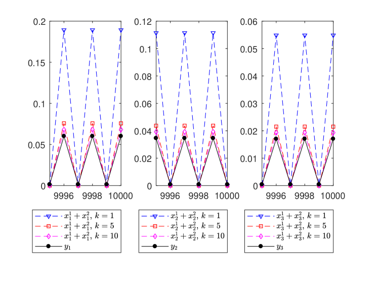
Figure 2: Comparison between the complete and the reduced systems. Total population corresponding to certain initial conditions for system (18) and for system (16) for three different values of $k$, i.e., $k\in\{1,5,10\}$. The simulations have been run until time $t=10^{4}$ and only the last 6 times are shown.
Parameter values: $s_{1}^{1}=0.3$, $s_{2}^{1}=0.47$, $s_{3}^{1}=0.7$, $s_{1}^{2}=s_{2}^{2}=s_{3}^{2}=0.5$, $\phi^{1}=3.8$, $\phi^{2}=3.5$, $c_{1}=c_{2}=1$, $d_{1}=5.3$, $d_{2}=5.6$, $v_{1}^{1}=0.3$, $v_{2}^{1}=0.25$, $v_{3}^{1}=0.1$. Initial condition: $X(0)=(0.02,0.02,0.05,0.05,0.02,0.02)$.

4.1 The effect of fast dispersal

The effect of dispersal in populations and in particular its effect at a global level when local isolated populations are connected, has considerable biological interest and has been addressed in a number of different contexts (see Jang and Mitra (2000); Yakubu (2008); Franco and Ruiz-Herrera (2015) among others). In this section we deal with models (15) and (16) and present some results that show how dispersal can change the two main asymptotic issues regarding the dynamics of the population. The first one is the survival of the population as reflected by the extinction equilibrium stability. Then, once the survival threshold is attained, we address the second issue, i.e., the tendency of the population towards either reproductive synchrony or asynchrony, represented by the stability of synchronous 2-cycles or positive equilibria, respectively.

We compare the outcomes of local (isolated sites) and global (dispersal interconnected sites) population dynamics. The reduction procedure applied to systems (15) and (16) allows us to use the corresponding reduced systems (17) and (18) to study their asymptotic behaviour. So, we use quantities $\bar{R}_{0}$ (resp. $\tilde{R}_{0}$) and $\bar{a}_{-}$ (resp. $\tilde{a}_{-}$) to characterize, respectively, survival and reproductive synchrony at the global level in the two systems. The influence of fast dispersal in the population dynamics is reflected through the values $v_{i}^{\alpha}$ that appear in the coefficients of matrices $\bar{H}(Y)$ (17) and $\tilde{H}(Y)$ (18). We recall that $V_{i}=(v_{i}^{1},v_{i}^{2})^{\mathsf{T}}$ ($i=1,2,3$) is the dominant probability normed eigenvector of matrix $M_{i}$ and therefore its components represent the equilibrium distribution of dispersal for individuals of class $i$, i.e, $v_{i}^{j}$ is the proportion of individuals of class $i$ present in patch $j$ after dispersal has reached equilibrium. Their value is

$$v_{i}^{1}=\frac{q_{i}}{p_{i}+q_{i}},\ v_{i}^{2}=\frac{p_{i}}{p_{i}+q_{i}},$$

where $p_{i}$ (resp. $q_{i})$ is the migration rate from patch one to patch two (resp. from patch two to patch one) for individuals of class $i$.

At the local level, i.e., if patches $\alpha=1,2$ are considered isolated, the matrix representing the population dynamics in each of them is

$$\mathbf{D}^{\alpha}(Y)=\left(\begin{array}[c]{ccc}0&s_{2}^{\alpha}\phi^{\alpha}\dfrac{1}{1+c^{\alpha}y_{2}^{\alpha}}&0\\ s_{1}^{\alpha}&0&s_{3}^{\alpha}\dfrac{1}{1+d^{\alpha}y_{2}^{\alpha}}\\ 0&s_{2}^{\alpha}&s_{3}^{\alpha}\left(1-\dfrac{1}{1+d^{\alpha}y_{2}^{\alpha}}\right)\\ &&\end{array}\right)$$ (23)

Effect of dispersal on extinction. The stability of the extinction equilibrium is locally determined by the corresponding inherent NRR

$$R_{0}^{\alpha}:=\frac{\phi^{\alpha}s_{1}^{\alpha}s_{2}^{\alpha}}{1-s_{2}^{\alpha}s_{3}^{\alpha}},\ \alpha=1,2,$$ (24)

and the tendency towards reproductive synchrony or asynchrony by

$$a_{-}^{\alpha}:=-(1-s_{2}^{\alpha}s_{3}^{\alpha})s_{1}^{\alpha}c^{\alpha}+s_{1}^{\alpha}s_{2}^{\alpha}s_{3}^{\alpha}(1-s_{3}^{\alpha})d^{\alpha},\ ~{}\alpha=1,2.$$ (25)

If we consider homogeneous sites concerning survival and fertility, i.e., $s_{i}^{1}=s_{i}^{2}=:s_{i}$ for $i=1,2,3$ and $\phi^{1}=\phi^{2}=:\phi$, we obtain that

$$R_{0}^{1}=R_{0}^{2}=\bar{R}_{0}=\tilde{R}_{0}=\frac{\phi s_{1}s_{2}}{1-s_{2}s_{3}},$$ (26)

so that, in particular, the population survives or gets extinct locally if and only if it does globally.

On the other hand, differences in local parameters, i.e., $s_{1}^{1}$ vs. $s_{1}^{2}$ and $\phi^{1}$ vs. $\phi^{2},$ can result in different survival outcomes at the local and the global levels provided appropriate dispersal rates are chosen. In the next result we show that under certain conditions, adequate dispersal strategies can transform the local population extinction in isolated patches into global survival.

Proposition 4.

Let us assume $s_{i}^{1}=s_{i}^{2}=:s_{i}$ for $i=2,3$, $R_{0}^{1}<1$ and $R_{0}^{2}<1$. If $\max\{s_{1}^{1}\phi^{2},s_{1}^{2}\phi^{1}\}>(1-s_{2}s_{3})/s_{2}$ then there exist intervals $I_{1},I_{2}\subseteq[0,1]$ (resp. $\tilde{I}_{1},\tilde{I}_{2}\subseteq[0,1]$) such that $\bar{R}_{0}>1$ (resp. $\tilde{R}_{0}>1$) for $v_{1}^{1}\in I_{1}$ and $v_{2}^{1}\in I_{2}$ (resp. $v_{1}^{1}\in\tilde{I}_{1}$ and $v_{2}^{1}\in\tilde{I}_{2}$).

Proof.

Let us assume, without loss of generality, that $s^{1}_{1}\phi^{2}\geq s^{2}_{1}\phi^{1}$ and use that $v_{i}^{2}=1-v_{i}^{1}$ for $i=1,2,3$ to obtain

$$\begin{array}[c]{rcl}\bar{R}_{0}&=&\dfrac{s_{2}}{1-s_{2}s_{3}}\left(v_{1}^{1}s^{1}_{1}+(1-v_{1}^{1})s^{2}_{1}\right)\left(v_{2}^{1}\phi^{1}+(1-v_{2}^{1})\phi^{2}\right)\\ &>&\dfrac{s_{2}}{1-s_{2}s_{3}}v_{1}^{1}(1-v_{2}^{1})s^{1}_{1}\phi^{2}.\end{array}$$

This last expression considered as function of variables $v_{1}^{1}$ and $v_{2}^{1}$ is continuous and takes the value $s^{1}_{1}\phi^{2}s_{2}/(1-s_{2}s_{3})>1$ for $v_{1}^{1}=1$ and $v_{2}^{1}=0$. This yields the existence of the intervals $I_{1},I_{2}\subseteq[0,1]$ that ensure $\bar{R}_{0}>1$ for $(v_{1}^{1},v_{2}^{1})\in I_{1}\times I_{2}$.

The proof for $\tilde{R}_{0}>1$ is analogous. ∎

The previous result says that given certain (common) adult survival rates, if the juvenile survival rate in one of the patches together with the fertility rate in the other are large enough to sustain the population, then there exist appropriate dispersal rates to compensate poor local survival conditions.

The opposite result also holds. Adequately chosen dispersal rates, under appropriate conditions, can make two isolated viable populations go extinct when they are connected.

Proposition 5.

Let us assume $s_{i}^{1}=s_{i}^{2}=s_{i}$ for $i=2,3$, $R_{0}^{1}>1$ and $R_{0}^{2}>1$. If $\min\{s_{1}^{1}\phi^{2},s_{1}^{2}\phi^{1}\}<(1-s_{2}s_{3})/s_{2}$ then there exist intervals $I_{1},I_{2}\subseteq[0,1]$ (resp. $\tilde{I}_{1},\tilde{I}_{2}\subseteq[0,1]$) such that $\bar{R}_{0}<1$ (resp. $\tilde{R}_{0}<1$) for $v_{1}^{1}\in I_{1}$ and $v_{2}^{1}\in I_{2}$ (resp. $v_{1}^{1}\in\tilde{I}_{1}$ and $v_{2}^{1}\in\tilde{I}_{2}$).

Proof.

Analogous to the proof of Proposition 4. ∎

Effect of dispersal on reproductive synchrony. We now illustrate the influence of fast dispersal on the population’s reproductive synchrony. We do so in the particular case of homogenous patches, i.e., when all demographic parameters are the same in both patches:

$$s_{i}^{1}=s_{i}^{2}=:s_{i}\text{ for }i=1,2,3;\ \phi^{1}=\phi^{2}=:\phi;\ c^{1}=c^{2}=:c;\ d^{1}=d^{2}=:d.$$ (27)

Thus, the demographic local matrices coincide

$$\mathbf{D}^{1}(Y)=\mathbf{D}^{2}(Y)=\left(\begin{array}[c]{ccc}0&s_{2}\phi\dfrac{1}{1+cy_{2}}&0\\ s_{1}&0&s_{3}\dfrac{1}{1+dy_{2}}\\ 0&s_{2}&s_{3}\left(1-\dfrac{1}{1+dy_{2}}\right)\\ &&\end{array}\right),$$ (28)

but, due to the dispersal rates, are different from the demographic global matrices for systems (17) and (18)

$$\rule{-12.91663pt}{0.0pt}\bar{H}(Y)=\left(\begin{array}[c]{ccc}0&s_{2}\phi\left(\dfrac{v_{2}^{1}}{1+cv_{2}^{1}y_{2}}+\dfrac{v_{2}^{2}}{1+cv_{2}^{2}y_{2}}\right)&0\\ \rule{0.0pt}{17.22217pt}s_{1}&0&s_{3}\left(\dfrac{v_{3}^{1}}{1+dv_{2}^{1}y_{2}}+\dfrac{v_{3}^{2}}{1+dv_{2}^{2}y_{2}}\right)\\ \rule{0.0pt}{17.22217pt}0&s_{2}&s_{3}\left(1-\left(\dfrac{v_{3}^{1}}{1+dv_{2}^{1}y_{2}}+\dfrac{v_{3}^{2}}{1+dv_{2}^{2}y_{2}}\right)\right)\\ &&\end{array}\right)$$ (29)

and

$$\rule{-25.83325pt}{0.0pt}\tilde{H}(Y)=\left(\begin{array}[c]{ccc}0&s_{2}\phi\left(\dfrac{v_{2}^{1}}{1+cs_{2}v_{2}^{1}y_{2}}+\dfrac{v_{2}^{2}}{1+cs_{2}v_{2}^{2}y_{2}}\right)&0\\ \rule{0.0pt}{17.22217pt}s_{1}&0&s_{3}\left(\dfrac{v_{3}^{1}}{1+ds_{2}v_{2}^{1}y_{2}}+\dfrac{v_{3}^{2}}{1+ds_{2}v_{2}^{2}y_{2}}\right)\\ \rule{0.0pt}{17.22217pt}0&s_{2}&s_{3}\left(1-\left(\dfrac{v_{3}^{1}}{1+ds_{2}v_{2}^{1}y_{2}}+\dfrac{v_{3}^{2}}{1+ds_{2}v_{2}^{2}y_{2}}\right)\right)\\ &&\end{array}\right)$$

As we pointed out in (26), these four matrices have the same inherent NRNs, $R_{0}^{1}=R_{0}^{2}=\bar{R}_{0}=\tilde{R}_{0}=\phi s_{1}s_{2}/(1-s_{2}s_{3})$, that we assume to be larger than 1. Then, the local reproductive synchrony at both patches is determined by the sign of (24)

$$a_{-}=s_{1}s_{2}s_{3}(1-s_{3})d-(1-s_{2}s_{3})s_{1}c,$$ (30)

the global reproductive synchrony in the case of system (15) by the sign of $\bar{a}_{-}$ in (21)

$$\bar{a}_{-}=s_{1}s_{2}s_{3}(1-s_{3})d\left(v_{2}^{1}v_{3}^{1}+(1-v_{2}^{1})(1-v_{3}^{1})\right)-(1-s_{2}s_{3})s_{1}c\left((v_{2}^{1})^{2}+(1-v_{2}^{1})^{2}\right),$$ (31)

and in the case of system (16) by the sign of $\tilde{a}_{-}$ (22). Note that $\tilde{a}_{-}=s_{2}\bar{a}$ and so the sign of $\tilde{a}_{-}$ coincides with that of $\bar{a}_{-}$, so that we will concentrate on the sign of $\bar{a}_{-}$.

Therefore, in order to illustrate the influence of fast dispersal on reproductive synchrony for both systems (17) and (18), we have to find conditions on $v_{2}^{1}$ and $v_{3}^{1}$ (note that $v_{1}^{1}$ plays no role whatsoever) such that $a_{-}$ and $\bar{a}_{-}$ have different signs. In that way we show that adequately chosen adult dispersal rates can alter the tendency to reproductive synchrony or asynchrony of isolated populations.

A first result shows that it is always possible to find adult dispersal rates such that there exists global reproductive asynchrony, $\bar{a}_{-}<0$, independently of the local tendency.

Proposition 6.

Let the model coefficients verify conditions (27). Then there exist intervals $I_{2},I_{3}\subseteq[0,1]$ such that $\bar{a}_{-}<0$ for $(v_{2}^{1}\in I_{2}$ and $v_{3}^{1})\in I_{3}$.

Proof.

The expression (31) of $\bar{a}_{-}$ taken as a function of $v_{2}^{1}$ and $v_{3}^{1}$, $\bar{a}_{-}(v_{2}^{1},v_{3}^{1})$, is continuous and satisfies $\bar{a}_{-}(1,0)=-(1-s_{2}s_{3})s_{1}c<0$, what implies the existence of the intervals $I_{2}$ and $I_{3}$ meeting the required conditions. ∎

This result proves that the local reproductive synchrony, $a_{-}>0$, can always be changed into global reproductive asynchrony, $\bar{a}_{-}<0$, through the appropriate adult dispersal rates. This fact is illustrated in Figure 3.

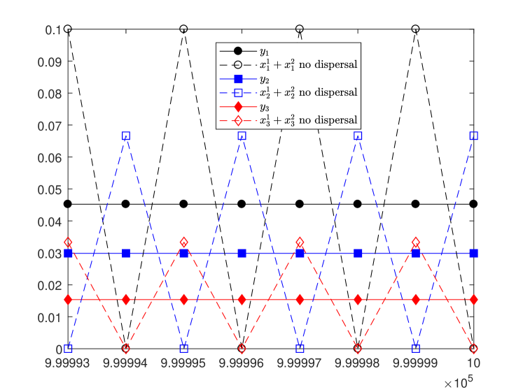
Figure 3: Changing local reproductive synchrony into global reproductive asynchrony. Change from local reproductive synchrony to global reproductive asynchrony in the adults reproductive behavior when going from the local level (isolated identical patches that have dynamics defined by matrices (28)) to the global level (represented by system (29)) when we incorporate dispersal.
Top: parameter values $s_{1}=s_{2}=s_{3}=0.5$, $c=1$, $d=10$, $\phi=3.1$, $v_{1}^{1}=0.3$, $v_{2}^{1}=7/8,\ v_{3}^{1}=1/8$.
Initial conditions are $X(0)=(0.02,0.02,0.05,0.05,0.02,0.02)$. The simulations have been run until time $t=10^{6}$ and only the last 8 times are shown.

In the opposite sense we present the next result in which we provide sufficient conditions so that the local reproductive asynchrony, $a_{-}<0$, can be changed into global reproductive synchrony, $\bar{a}_{-}>0$, if adult dispersal is adequately chosen.

Proposition 7.

Let the model coefficients verify conditions (27) and $a_{-}<0$. Then, there exist intervals $I_{2},I_{3}\subseteq[0,1]$ such that $\bar{a}_{-}>0$ for $v_{2}^{1}\in I_{2}$, $,v_{3}^{1}\in I_{3}$ if and only if

$$(1-s_{2}s_{3})s_{1}c<\frac{1+\sqrt{2}}{2}s_{1}s_{2}s_{3}(1-s_{3})d.$$

Proof.

The expression (31) of $\bar{a}_{-}$ taken as a function of $v_{2}^{1}$ and $v_{3}^{1}$, $\bar{a}_{-}(v_{2}^{1},v_{3}^{1})$, is continuous and satisfies

$$\begin{array}[c]{rcl}\bar{a}_{-}(1-\dfrac{\sqrt{2}}{2},0)&=&s_{1}s_{2}s_{3}(1-s_{3})d\dfrac{\sqrt{2}}{2}-(1-s_{2}s_{3})s_{1}c(4-2\sqrt{2})\\ &=&(4-2\sqrt{2})\left(s_{1}s_{2}s_{3}(1-s_{3})d\dfrac{1+\sqrt{2}}{2}-(1-s_{2}s_{3})s_{1}c\right)>0,\end{array}$$

what implies the existence of the intervals $I_{2}$ and $I_{3}$ meeting the required conditions.

In the opposite sense, if we assume, by contradiction, that

$$(1-s_{2}s_{3})s_{1}c\geq\dfrac{1+\sqrt{2}}{2}s_{1}s_{2}s_{3}(1-s_{3})d$$

and $\bar{a}_{-}>0$ then

$$\dfrac{1+\sqrt{2}}{2}\leq\frac{(1-s_{2}s_{3})s_{1}c}{s_{1}s_{2}s_{3}(1-s_{3})d}<\frac{v_{2}^{1}v_{3}^{1}+(1-v_{2}^{1})(1-v_{3}^{1})}{(v_{2}^{1})^{2}+(1-v_{2}^{1})^{2}}$$

but there are no $v_{2}^{1},v_{3}^{1}\in[0,1]$ satisfying the previous inequality since the maximum of function $f(x,y)=(xy+(1-x)(1-y))/(x^{2}+(1-x)^{2})$ on $[0,1]\times[0,1]$ is $(1+\sqrt{2})/2$. ∎

This change from local reproductive asynchrony to global reproductive synchrony in the adults reproductive behavior for adequate dispersal parameters is illustrated in Figure (4)

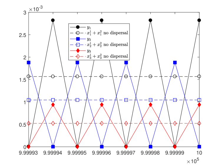
Figure 4: Changing local reproductive asynchrony into global reproductive synchrony. Change from local reproductive asynchrony to global reproductive synchrony in the adults reproductive behavior when going from the local level (isolated identical patches that have dynamics defined by matrices (28)) to the global level (represented by system (29)) when we incorporate dispersal.
Parameter values: $s_{1}=s_{2}=s_{3}=0.5$, $c=1$, $d=5.5$, $\phi=3.0003$, $v_{1}^{1}=0.3,\ v_{2}^{1}=3/8,\ v_{3}^{1}=1/8$.
Initial conditions are $X(0)=(0.02,0.02,0.05,0.05,0.02,0.02)$. The simulations have been run until time $t=10^{6}$ and only the last 8 times are shown.

The preceding behavior, in which if appropriate adult dispersal rates are chosen, the existence of a positive locally asymptotically stable equilibrium locally in each site can be transformed globally into the existence of a stable 2-cycle and viceversa, is analogous to the one found in Bravo de la Parra et al. (2016) for a semelparous population structured in juveniles and adults, spread out in two patches between which they can migrate.

4.2 Differences between models (15) and (16).

In this section we propose some particular simple settings in which the asymptotic outcomes of systems (15) and (16) differ, thus showing that the decision of placing mortality at the slow or the fast time scale can have crucial consequences.

There is a simple case in which the inherent NRNs $\bar{R}_{0}$ and $\tilde{R}_{0}$, associated to systems (15) and (16), coincide. Indeed, if $s_{i}^{1}=s_{i}^{2}=:s_{i}$, for $i=1,2,3$, then

$$\tilde{R}_{0}=\frac{s_{1}s_{2}\left(\phi^{1}v_{2}^{1}+\phi^{2}v_{2}^{2}\right)}{1-s_{2}s_{3}}=\bar{R}_{0}.$$

In the next result we show that equal fertilities, $\phi^{1}=\phi^{2}$, imply that $\bar{R}_{0}$ is larger than $\tilde{R}_{0}$.

Proposition 8.

In systems (15) and (16), if $\phi^{1}=\phi^{2}=:\phi$ then

$$\tilde{R}_{0}<\bar{R}_{0}.$$

Moreover, there is an interval $I\in\mathbb{R}_{+}$ such that if $\phi\in I$ then

$$\tilde{R}_{0}<1<\bar{R}_{0}.$$ (32)

Proof.

If we use the fact that, for $i=1,2,3$, we have $v_{i}^{1},v_{i}^{2}\in(0,1)$ and $v_{i}^{1}+v_{i}^{2}=1$, the inequality relating the weighted arithmetic mean and the weighted geometric mean implies that the survival rates in (17) and (18) verify

$$\tilde{s}_{i}=\left(s_{i}^{1}\right)^{v_{i}^{1}}\left(s_{i}^{2}\right)^{v_{i}^{2}}<s_{i}^{1}v_{i}^{1}+s_{i}^{2}v_{i}^{2}=\bar{s}_{i},$$

and the fertility coefficients

$$\tilde{b}=\tilde{s}_{2}\left(\phi v_{2}^{1}+\phi v_{2}^{2}\right)=\tilde{s}_{2}\phi<\bar{s}_{2}\phi=\phi s_{2}^{1}v_{2}^{1}+\phi s_{2}^{2}v_{2}^{2}=\bar{b}.$$

Now, it is straightforward that

$$\tilde{R}_{0}=\frac{\tilde{b}\tilde{s}_{1}}{1-\tilde{s}_{2}\tilde{s}_{3}}<\frac{\bar{b}\bar{s}_{1}}{1-\bar{s}_{2}\bar{s}_{3}}=\bar{R}_{0}$$

Inequality (32) is a direct consequence of both $\tilde{R}_{0}$ and $\bar{R}_{0}$ depending linearly on $\phi$. ∎

We stress that choosing one of models (15) and (16) over the other can represent the difference between population survival or extinction.

We now present a situation in which the inequalities in Proposition 8 are reversed. We assume that $s_{1}^{1}=s_{1}^{2}=s_{1}$, $s_{1}^{2}=0.7$, $s_{2}^{2}=0.5$, $s_{3}^{1}=s_{3}^{2}=0.8$, $v_{2}^{1}=v_{2}^{2}=0.5$, $\phi^{1}=\phi$ and $\phi^{2}=\alpha\phi$. Straightforward calculations yield

$$\tilde{R}_{0}-\bar{R}_{0}=s_{1}\phi\left(\left(\frac{5\sqrt{35}}{100-8\sqrt{35}}-\frac{25}{52}\right)\alpha+\frac{5\sqrt{35}}{100-8\sqrt{35}}-\frac{35}{52}\right),$$

therefore, for $\alpha>\dfrac{65\sqrt{35}+14}{289}$ we have $\bar{R}_{0}<\tilde{R}_{0}$. As this hold for any values of $s_{1}\in(0,1)$ and $\phi>0$, there are some of them for which

$$\bar{R}_{0}<1<\tilde{R}_{0},$$

which represents the difference between population survival or extinction but exchanging the associated models in Proposition 8.

It can be shown that, similarly to what happens regarding survival, there exist situations where models (15) and (16) have different outputs regarding the population reproductive synchrony. Nevertheless, we skip this analysis since we consider that the previous results illustrate clearly our main point here: the choice of model should be as accurate as possible because the results can drastically differ.

5 Discussion

In this work we have extended the results on reduction of two time scales non linear discrete systems presented in Sanz et al. (2008). The new result avoids the need to check a difficult hypothesis, specifically the uniform convergence on compacts sets of the differentials of the iterates of a map. The dropping this hypothesis has an effect on the results that can be given regarding the relationships between the original and the reduced model, but nonetheless can be viewed as a minor effect with regard to the practical study of population dynamics models.

This new result has opened the door to extending to the nonlinear case the work on re-scaling developed in Nguyen-Huu et al. (2011). When there are two processes acting at different time scales that must be gathered in a single discrete model, the easiest choice of its time unit is that associated to the slow one. The structure of the model then reflects that the fast process acts a number of times, approximately equal to the ratio between the two time scales, followed by one action of the slow process. It is not always easy to decide if a process occurs at the slow or the fast time scale. Here we have focussed on the re-scaling of survival, which is a process usually measured at the slow time scale associated to the rest of the demographic processes. Nevertheless, in a context of fast movements of individuals between patches with different associated survival rates, it can be argued that it should be rather considered as occurring at the fast time scale. Systems (15) and (16) represent general discrete time models of structured metapopulations with two time scales; in the first one survival acts at the slow time scale and in the second one the re-scaled survival acts at the fast time scale. The reduction results developed in Sections (2) and (3) associated to these two models yield two aggregated models, (17) and (18), that contain the asymptotic information of the original models. They summarize the global emergent properties Auger et al. (2008a); Auger and Poggiale (1998) that fast dispersal induce out of local demography.

To illustrate this influence of fast dispersal on local demographic dynamics and the relevance of the choice of time scale for the different processes involved in a model, we have proposed a particular case of systems (15) and (16). It is based in the model in Veprauskas and Cushing (2017) and it has three population stages and two patches. The comparison of the local models and the two global models is done through their respective inherent net reproduction numbers, that decide on the survival or extinction of the population, and the coefficients $a_{-}$ that rule, for viable populations, the tendency to either reproductive synchrony or asynchrony. Even in simple cases it can be shown that viable local populations can get globally extinct for adequate dispersal rates and, the other way round, non viable local populations can globally survive if migrating appropriately. Along the same lines, different scenarios are presented reversing the outcome of reproductive synchrony/asynchrony between local and global dynamics.

Finally, it is shown that there are some cases where changing from system (15) to (16) (or viceversa) can represent changing the global outcome from survival to extinction or the other way round. This fact stresses the importance of the choice of time scale (slow ar fast) in which survival is included in the model.

It must be stressed that the result in Theorem 2 can be applied to much more general systems than the specific structured metapopulation models presented in Section 3. Also, the convergence results in Proposition 10 have a more general application than the survival re-scaling proposed in this work. We have chosen the context of the work trying to keep at reasonable levels both simplicity and modelling relevance.

An interesting extension of the treated metapopulation models would also include an epidemic disease dynamics together with the demographic and spatial issues. These more general models would encompass time scales too. A relevant issue at this point would be to decide whether the epidemic process must be considered as acting as at the fast or the slow time scale. In case that it be considered as a slow process together with demography, the reduction of the corresponding two time scales system would not differ much from what has been developed in this work since it mainly depends on the fast process. On the other hand, a general assumption in basic epidemic models is that disease evolution can be considered almost instantaneous with respect to demography and therefore this latter is considered negligible. A different approach to this last assumption is considering in the same model both disease and demographic dynamics at different time scales. The obtained two-time scale systems would be susceptible of reduction. The inclusion of disease dynamics in the fast part of the system would render the reduction procedure more involved, and Theorem 1 should be a tool helping in this task.

Appendix A Appendix

Lemma 9.

Let Hypotheses 1 and 3 hold. Then for any $m\in\mathbb{N}$ we have $\lim_{k\rightarrow\infty}H_{k}^{m}=H^{m}$ uniformly on compact sets of $\Omega_{N}$.

Proof.

It is easy to realize that it suffices with proving the result for $m=2$.

Let $M\subset\Omega_{n}$ be a compact set. Since $\lim_{k\rightarrow\infty}H_{k}=H$ uniformly on $M$, we can find another compact set $C\subset\Omega_{n}$ and $k^{*}\in\mathbb{N}$ such that $H(M)\subset C$ and $H_{k}(M)\subset C$ for all $k\geq k^{*}$.

Let us now show that $\lim_{k\rightarrow\infty}H_{k}^{2}=H^{2}$ uniformly on $K$.

The uniform convergence $\lim_{k\rightarrow\infty}H_{k}=H$ on $C$ assures the existence of a real sequence $\left\{\alpha_{k}\right\}_{k\in\mathbb{N}}$, $\alpha_{k}>0$, with $\lim_{k\rightarrow\infty}\alpha_{k}=0$ and such that $\sup_{X\in C}\left\|H_{k}(X)-H(X)\right\|\leq\alpha_{k}$. Since

$$\left\|H_{k}^{2}(X)-H^{2}(X)\right\|\leq\left\|H_{k}(H_{k}(X))-H(H_{k}(X\mathbf{)})\right\|+\left\|H(H_{k}(X))-H(H(X\mathbf{)})\right\|,$$

we have, for $k\geq k^{\ast}$, that

$$\underset{X\in M}{\sup}\left\|H_{k}^{2}(X)-H^{2}(X)\right\|\leq\underset{Z\in C}{\sup}\left\|H_{k}(Z)-H(Z)\right\|+\sup_{{\tiny\begin{array}[c]{c}Z_{k},Z\in C\\ \left\|Z_{k}-Z\right\|\leq\alpha_{k}\end{array}}}\left\|H(Z_{k})-H(Z)\right\|.$$

When $k\rightarrow\infty$, the first term on the right-hand side converges to zero due to the uniform convergence of $H_{k}$ to $H$ on $C$ and the second term converges to zero since $H$ is uniformly continuous on $C$. Therefore the result is proved. ∎

Proposition 10.

Let $I,J\in\mathbb{Z}_{+}$ and let $\Omega\subset\mathbb{R}^{I}$ be an open set. Let $M:\Omega\rightarrow\mathbb{R}^{J\times J}$ and $S:\Omega\rightarrow\mathbb{R}^{J\times J}$ be continuous maps such that:

a. For all $Y\in\Omega$, $M(Y)$ is a primitive probability matrix. Let $v(Y)$ be its column Perron right eigenvector normalized so that $\mathbf{1}v(Y)=1$.

b. There exists a continuous map $S^{\prime}:\Omega\rightarrow\mathbb{R}^{J\times J}$ such that $\exp\left(S^{\prime}(Y)\right)=S(Y)$ for all $Y\in\Omega$.

Let us define, for $Y\in\Omega$, $S_{k}(Y):=\exp\left(\frac{1}{k}S^{\prime}(Y)\right)$, $\bar{M}(Y):=v(Y)\mathbf{1}$ and $\gamma(Y):=\exp\left(\mathbf{1}S^{\prime}(Y)v(Y)\right)$. Then we have

$$\lim_{k\rightarrow\infty}\left(S_{k}(Y)M(Y)\right)^{k}=\lim_{k\rightarrow\infty}\left(M(Y)S_{k}(Y)\right)^{k}=\gamma(Y)\bar{M}(Y)$$ (33)

where the limit is uniform on any compact set of $\Omega$.

Proof.

Given a fixed $Y\in\Omega$, matrix $M(Y)$ is primitive, its (strictly) dominant eigenvalue is 1 and its associated left eigenvector $u(Y),$ normalized so that $u(Y)^{T}v(Y)=1,$ is $u(Y)=\mathbf{1}$. Then, the existence of the pointwise limit (33) follows as a particular case of Theorem A1 in Nguyen-Huu et al. (2011). Therefore, all we need to prove is that limit (33) is uniform on compact sets of $\Omega$.

We only need to adjust some details at the beginning of the proof of Theorem A1 in Nguyen-Huu et al. (2011) to make it work in the present case via standard compactness arguments. Let $|\rule{-1.72218pt}{0.0pt}|\rule{-1.72218pt}{0.0pt}|\ |\rule{-1.72218pt}{0.0pt}|\rule{-1.72218pt}{0.0pt}|$ be the 1-norm in $\mathbb{R}^{J\times J}$. In the first place, since the $M(Y)$ are probability matrices one has

$$|\rule{-1.72218pt}{0.0pt}|\rule{-1.72218pt}{0.0pt}|M(Y)|\rule{-1.72218pt}{0.0pt}|\rule{-1.72218pt}{0.0pt}|=1$$ (34)

for all $Y\in\Omega$. Now let $K\subset\Omega$ be any compact set. For any $Y^{\prime}\in K$ there exists $r_{Y^{\prime}}<1$ such that $|\rule{-1.72218pt}{0.0pt}|\rule{-1.72218pt}{0.0pt}|M(Y^{\prime})-\bar{M}(Y^{\prime})|\rule{-1.72218pt}{0.0pt}|\rule{-1.72218pt}{0.0pt}|<r_{Y^{\prime}}$. The continuity of $M$ and of the norm imply that if $\bar{r}_{Y^{\prime}}$ satisfies $r_{Y^{\prime}}<\bar{r}_{Y^{\prime}}<1$, there exists an open neighbourhood of $Y^{\prime}$ in $\Omega$, $\mathcal{U}_{Y^{\prime}}$, such that

$$|\rule{-1.72218pt}{0.0pt}|\rule{-1.72218pt}{0.0pt}|M(Y)-\bar{M}(Y)|\rule{-1.72218pt}{0.0pt}|\rule{-1.72218pt}{0.0pt}|<\bar{r}_{Y^{\prime}}\text{ for all }Y\in\mathcal{U}_{Y^{\prime}}.$$ (35)

Let $\delta>0$ and let us denote

$$\left(\delta S(Y)\right)^{\prime} :=S^{\prime}(Y)+\log\delta I$$

$$\left(\delta S(Y)\right)_{k} :=\exp(\frac{1}{k}\left(\delta S(Y)\right)^{\prime}),\ \gamma_{\delta S}(Y):=\exp\left(\mathbf{1}\left(\delta S(Y)\right)^{\prime}v(Y)\right)$$

It is immediate to check that $\left(\delta S(Y)\right)_{k}=\delta^{\frac{1}{k}}S_{k}(Y)$ and $\gamma_{\delta S}(Y)=\delta\gamma(Y).$ Therefore

$$\left(\left(\delta S(Y)\right)_{k}M(Y)\right)^{k}-\gamma_{\delta S}(Y)=\delta\left(S_{k}(Y)M(Y)-\gamma(Y)\right)^{k}$$

so that the limit (33) is uniform in $K$ if and only if there exists $\delta>0$ such that the limit $\lim_{k\rightarrow\infty}\left(\left(\delta S(Y)\right)_{k}M(Y)\right)^{k}=\gamma_{\delta S}(Y)$ is uniform in $K$. Now let $\delta:=\min_{Y\in\mathcal{\bar{U}}_{Y^{\prime}}}\exp\left(-|\rule{-1.72218pt}{0.0pt}|\rule{-1.72218pt}{0.0pt}|S^{\prime}(Y)|\rule{-1.72218pt}{0.0pt}|\rule{-1.72218pt}{0.0pt}|\right)>0$. Then,

$$|\rule{-1.72218pt}{0.0pt}|\rule{-1.72218pt}{0.0pt}|\left(\delta S(Y)\right)_{k}|\rule{-1.72218pt}{0.0pt}|\rule{-1.72218pt}{0.0pt}|=\delta^{\frac{1}{k}}|\rule{-1.72218pt}{0.0pt}|\rule{-1.72218pt}{0.0pt}|\exp\left(\frac{1}{k}S^{\prime}(Y)\right)|\rule{-1.72218pt}{0.0pt}|\rule{-1.72218pt}{0.0pt}|\leq 1$$

and so we can assume, without loss of generality, that $|\rule{-1.72218pt}{0.0pt}|\rule{-1.72218pt}{0.0pt}|S_{k}(Y)|\rule{-1.72218pt}{0.0pt}|\rule{-1.72218pt}{0.0pt}|\leq 1$ for all $Y\in\mathcal{U}_{Y^{\prime}}$ and all $k=1,2,...$, from where it follows that

$$|\rule{-1.72218pt}{0.0pt}|\rule{-1.72218pt}{0.0pt}|\left(M(Y)S_{k}(Y)\right)^{i}|\rule{-1.72218pt}{0.0pt}|\rule{-1.72218pt}{0.0pt}|\leq|\rule{-1.72218pt}{0.0pt}|\rule{-1.72218pt}{0.0pt}|M(Y)|\rule{-1.72218pt}{0.0pt}|\rule{-1.72218pt}{0.0pt}|^{i}|\rule{-1.72218pt}{0.0pt}|\rule{-1.72218pt}{0.0pt}|S_{k}(Y)|\rule{-1.72218pt}{0.0pt}|\rule{-1.72218pt}{0.0pt}|^{i}=|\rule{-1.72218pt}{0.0pt}|\rule{-1.72218pt}{0.0pt}|S_{k}(Y)|\rule{-1.72218pt}{0.0pt}|\rule{-1.72218pt}{0.0pt}|^{i}\leq 1$$ (36)

for all $Y\in\mathcal{U}_{Y^{\prime}}$ and $i,k\in\mathbb{N}.$ Thus, from (34), (35) and (36) the rest of the proof of Theorem A1 in Nguyen-Huu et al. (2011) is valid (in the particular case of working with the 1-matrix norm) and yields that limit (33) is uniform on $\mathcal{U}_{Y^{\prime}}$. A standard compactness argument ensures the uniform convergence on $K$ and completes the proof.

∎

Competing interests

The authors declare that they have no competing interests.

Author’s contributions

All authors have the same contributions. All authors read and approved the final manuscript.

Funding

This work was supported by Ministerio de Economía y Competitividad (Spain), project MTM2014-56022-C2-1-P.

References

• Auger and Poggiale (1998) Auger, A., Poggiale, J., 1998. Aggregation and emergence in systems of ordinary differential equations. Mathematical and Computer Modelling 27, 1–22.
• Auger and Lett (2003) Auger, P., Lett, C., 2003. Integrative biology: linking levels of organization. Comptes Rendus de l’Académie des Sciences de Paris, Biology 326, 517–522.
• Auger et al. (2008a) Auger, P., Bravo de la Parra, R., Poggiale, J.C., Sánchez, E., Nguyen-Huu, T., 2008a. Aggregation of variables and applications to population dynamics, in: Structured population models in biology and epidemiology. Springer, Berlin, pp. 209–263.
• Auger et al. (2008b) Auger, P., Bravo de la Parra, R., Poggiale, J.C., Sánchez, E., Sanz, L., 2008b. Aggregation methods in dynamical systems and applications in population and community dynamics. Physics of Life Reviews 5, 79–105.
• Border (1989) Border, K.C., 1989. Fixed point theorems with applications to economics and game theory. Cambridge university press, Cambridge.
• Cushing (2015) Cushing, J., 2015. Mathematics of Planet Earth: Dynamics, Games and Science. Springer, Berlin. chapter On the fundamental bifurcation theorem for semelparous Leslie models. CIM Mathematical Sciences Series, pp. 215–251.
• Cushing and Yicang (1994) Cushing, J., Yicang, Z., 1994. The net reproductive value and stability in matrix population models. Natural Resources Modeling 8, 297–333.
• Franco and Ruiz-Herrera (2015) Franco, D., Ruiz-Herrera, A., 2015. To connect or not to connect isolated patches. Journal of theoretical biology 370, 72–80.
• Jang and Mitra (2000) Jang, S.J., Mitra, A.K., 2000. Equilibrium stability of single-species metapopulations. Bulletin of mathematical biology 62, 155–161.
• LaSalle (1976) LaSalle, J.P., 1976. The stability of dynamical systems. volume 25. Siam, Philadelphia.
• Levin (1992) Levin, S., 1992. The problem of pattern and scale in ecology. Ecology 73, 1943–1967.
• Lischke et al. (2007) Lischke, H., et al., 2007. Up-scaling of biological properties and models to the landscape level.
• Marvá et al. (2013) Marvá, M., Moussaoui, A., Bravo de la Parra, R., Auger, P., 2013. A density-dependent model describing age-structured population dynamics using hawk–dove tactics. Journal of Difference Equations and Applications 19, 1022–1034.
• Marvá et al. (2009) Marvá, M., Sánchez, E., Bravo de la Parra, R., Sanz, L., 2009. Reduction of slow–fast discrete models coupling migration and demography. Journal of theoretical biology 258, 371–379.
• Nguyen-Huu et al. (2011) Nguyen-Huu, T., Bravo de la Parra, R., Auger, P., 2011. Approximate aggregation of linear discrete models with two time scales: re-scaling slow processes to the fast scale. Journal of Difference Equations and Applications 17, 621–635.
• Bravo de la Parra et al. (2013) Bravo de la Parra, R., Marvá, M., Sánchez, E., Sanz, L., 2013. Reduction of discrete dynamical systems with applications to dynamics population models. Mathematical Modelling of Natural Phenomena 8, 107–129.
• Bravo de la Parra et al. (2016) Bravo de la Parra, R., Marvá, M., Sansegundo, F., 2016. Fast dispersal in semelparous populations. Mathematical Modelling of Natural Phenomena 11, 120–134.
• Sanz et al. (2008) Sanz, L., Bravo de la Parra, R., Sánchez, E., 2008. Approximate reduction of non-linear discrete models with two time scales. Journal of Difference Equations and Applications 14, 607–627.
• Veprauskas and Cushing (2017) Veprauskas, A., Cushing, J.M., 2017. A juvenile–adult population model: climate change, cannibalism, reproductive synchrony, and strong allee effects. Journal of biological dynamics 11, 1–24.
• Yakubu (2008) Yakubu, A.A., 2008. Asynchronous and synchronous dispersals in spatially discrete population models. SIAM Journal on Applied Dynamical Systems 7, 284–310.