Spacecraft Rendezvous Guidance via Factorization-Free Sequential Convex Programming using a First-Order Method

Abstract

We implement a fully factorization-free algorithm for nonconvex, free-final-time trajectory optimization. This algorithm is based on sequential convex programming and utilizes an inverse-free, exact discretization procedure to ensure dynamic feasibility of the converged trajectory and PIPG, a fast, first-order conic optimization algorithm as the subproblem solver. Although PIPG requires the tuning of a hyperparameter to achieve fastest convergence, we show that PIPG can be tuned to a nominal trajectory optimization problem and it is robust to variations in initial condition. We demonstrate this with a monte carlo simulation of the free-final-time rendezvous problem, using Clohessy-Wiltshire dynamics, an impulsive thrust model, and various state and control constraints including a spherical keepout zone.

1 Notation

$0_{n}$	Matrix of zeros in $\mathbb{R}^{n\times n}$
$0_{n\times m},1_{n\times m}$	Matrix of zeros and ones respectively in $\mathbb{R}^{n\times m}$
$I_{n}$	Identity matrix in $\mathbb{R}^{n\times n}$
$V_{[1:n]}$	Collection of vectors or matrices $V_{k}$, for $k=1,\ldots,n$
$v_{i}$	Element $i$ of vector $v$
$(u,v)$	Concatenation of vectors $u\in\mathbb{R}^{n}$ and $v\in\mathbb{R}^{m}$ to form a vector in $\mathbb{R}^{n+m}$
$[A\,B]$	Concatenation of matrices $A$ and $B$ with same number of rows

2 Introduction

The spacecraft rendezvous problem is concerned with finding a sequence of thrust commands and the resulting trajectory for a chaser spacecraft to bring it from some relative initial position and velocity with respect to a target spacecraft to the same final position as the target spacecraft with zero relative velocity. The trajectory and thrust commands must also satisfy a multitude of constraints such as maximum delta-v of the thrusters, maximum speed of the spacecraft, and potentially a keep-out zone.

This problem is becoming increasingly important as a number of upcoming spaceflight missions have rendezvous as a key component of their concept of operations (CONOPS). NASA is currently working on the Artemis program where they will attempt to establish long term presence on the moon [1]. For this project, NASA will be building the Lunar Gateway, which is a large space station in lunar orbit that will serve as a waypoint for missions from Earth to the lunar surface. SpaceX and Blue Origin have been contracted by NASA to build human lander systems (HLS), which will rendezvous with the Gateway in lunar orbit and transport astronauts to the lunar surface [2, 3]. Consequently, performing a rendezvous with the Gateway is mission critical for the Artemis program.

Additionally, with companies such as Vast and Axiom Space building private space stations in low earth orbit (LEO), the number of spacecraft rendezvous performed will increase [4, 5]. Furthermore, companies such as Starfish Space are building spacecrafts to service and deorbit satellites in LEO [6]. All of these projects necessitates the need for reliable algorithms to solve the rendezvous problem.

A natural way of solving for trajectories subject to many constraints is formulating a nonconvex optimal control problem and solving this problem using sequential convex programming (SCP) [7, 8]. This is a very capable solution method and can handle difficult discrete logic constraints such as minimum impulse bit for thrusters, distance triggered plume impingement constraints, and distance triggered approach-cone constraints [9, 10].

The SCP procedure requires an initial guess for the state and control trajectory. It then linearizes all nonconvex constraints and the nonlinear dynamics about this reference trajectory while keeping all convex constraints unchanged. Next, an exact discretization is performed using multiple shooting to formulate a convex subproblem which will update the reference trajectory. This subproblem can then be solved using off-the-shelf convex solvers. This process of linearization, discretization, and solving the resulting convex subproblem is repeated until convergence [7]. Upon convergence, the algorithm returns a dynamically feasible trajectory and control signal both of which satisfy the original constraints of the problem at the discrete nodes.

This solution procedure is agnostic to the solver used for the convex subproblem. If the subproblem is a second-order cone program (socp), open-source off-the-shelf solvers such as ecos and scs can be used [11, 12, 13]. If the subproblem is a quadratic program (qp), solvers such as osqp and piqp can be used in addition to the the aformentioned socp solvers [14, 15]. Typically the subproblem is a socp when constraints such as maximum speed or maximum thrust are imposed and ecos is typically used as the subproblem solver [10].

For safety critical systems such as human spaceflight, the convex solver software will need to undergo extensive testing and scrutiny in addition to verification of the underlying algorithm [16]. The ecos solver is a few thousand lines of code and leverages many complex features such as sparse, permuted Cholesky factorization, Nesterov-Todd scaling, and Mehrotra’s predictor-corrector [11, 17]. Fundementally understanding how this solver works requires advanced knowledge of numerical optimization which makes verification more challenging. Another downside of ecos is that we cannot warmstart it. In SCP, warmstarting the solution to one subproblem based on the solution to the previous subproblem will allow quicker convex solves, but we cannot do this when using ecos.

Alternatively, the Proportional-Integral Projected Gradient (pipg) algorithm is four lines of pseudocode and only uses matrix-vector multiplication and closed-form projections onto simple sets such as balls and boxes [18]. We can also warmstart pipg which allows it to solve convex subproblems quicker. The pipg algorithm has been used within the SCP framework to solve the multiphase Starship landing problem and the 6-DoF powered descent guidance problem with dual quaternions [19, 20]. In both cases, pipg was roughly three times faster than ecos. However, the downside of pipg is that it requires the tuning of the hyperparameter $\omega$, the dual to primal stepsize ratio, to maximize convergence speed.

In this paper we will solve a rendezvous problem with relevant constraints using the SCP framework with pipg as a subproblem solver and show that when this hyperparameter is properly tuned to a nominal problem, it is robust to variations in problem data such as variation in initial conditions.

3 Rendezvous Problem Formulation

In this section, we will formulate the free-final time, minimum control effort rendezvous problem that we will be considering in the rest of the paper.

3.1 Dynamics

We will begin by assuming that the target spacecraft is in a circular orbit and the chaser spacecraft is in an elliptical orbit. We can define a right handed Cartesian coordinate system whose origin is on the target spacecraft with unit vectors $\hat{i},\hat{j},\hat{k}$, such that $\hat{i}$ points radially outwards from the target body, $\hat{j}$ points in the direction of the velocity vector of the target body, and $\hat{k}$ points in the angular momentum direction of the target body’s orbit.

If the chaser spacecraft is sufficiently close to the target spacecraft, the equations of motion that govern the relative motion of the chaser spacecraft are the Clohessy-Wiltshire (CW) equations [21]. With the state vector defined as $x=[r^{\top}\;v^{\top}]^{\top}$ where $r$ is the position and $v$ is the velocity in the coordinate frame, and control input $u\in\mathbb{R}^{3}$ which is the applied force per unit mass, we can define the CW equations as follows

$$\dot{x}=f(x)+Bu=\begin{bmatrix}v_{1}\\ v_{2}\\ v_{3}\\ 3n^{2}r_{1}+2nv_{2}\\ -2nv_{1}\\ -n^{2}r_{3}\end{bmatrix}+\begin{bmatrix}0_{3\times 3}\\ I_{3}\end{bmatrix}u$$ (1)

where $n$ is the mean motion of the target body.

For this problem, we will model the control input as an impulse which will instantaneously change the velocity of the spacecraft. This model is valid when the amount of time taken for the spacecraft’s thrusters to change the spacecraft’s velocity is insignificant when compared to the total maneuver time.

If we define the change in velocity due to the thrusters for an impulsive burn as $u_{b}\in\mathbb{R}^{3}$ we can write the control input, $u(t)$, due to an impulse at $t_{b}$ as follows[22]

$$u(t)=u_{b}\delta(t-t_{b})$$ (2)

where $\delta(t)$ is the Dirac delta function.

3.2 Control Constraint

We will have a control constraint that places an upper bound on the magnitude of the impulse delivered by the engine. This constraint is driven by the maximum thrust the spacecraft’s propulsion system can provide. We can express this constraint as Equation 3 where $u_{\max}$ is the maximum delta-v the thrusters can provide.

$$\|u_{b}\|_{2}\leq u_{\max}$$ (3)

3.3 State Constraints

We will consider two state constraints: a spherical keepout zone, which can easily be generalized to an elliptical keepout zone, and a maximum speed constraint. Equation 4 describes these constraints, where $r_{c}\in\mathbb{R}^{3}$ is the center of the keepout zone, $\rho_{c}\in\mathbb{R}$ is the radius of the keepout zone, and $v_{\max}\in\mathbb{R}$ is the maximum speed. Note that the keepout zone constraint is nonconvex.

$$\|r(t)-r_{c}\|_{2}\geq\rho_{c}$$ (4a)

$$\|v(t)\|_{2}\leq v_{\max}$$ (4b)

3.4 Boundary Conditions

The initial conditions for the chaser spacecraft will be some arbitrary initial position and velocity, and the terminal condition will be at the target spacecraft with zero velocity. This can be expressed as follows

$$r(0) =r_{i}$$ (5a)

$$v(0) =v_{i}$$ (5b)

$$r(t_{f}) =0_{3\times 1}$$ (5c)

$$v(t_{f}) =0_{3\times 1}$$ (5d)

3.5 Continuous Time Nonconvex Optimal Control Problem

In this problem we are minimizing control effort. We could alternatively minimize fuel consumption if we did not square the argument of the integrand, or consider a minimum time problem by minimizing $t_{f}$. Note that since this problem is free final time, the time-of-flight, $t_{f}$, is an optimization variable. We can write the full continuous time nonconvex optimal control problem as follows

4 Sequential Convex Programming

In this section we will outline the sequential convex programming procedure which we will use to cast the continuous time nonconvex optimal control problem in the previous section into a sequence of finite dimensional convex subproblems. We will adopt the SCP procedure outlined by Malyuta et al [7], but will use time interval dilation from Kamath et al [19] and Berning et al [8] and an inverse-free discretization procedure discussed by Kamath et al[19].

4.1 Time Interval Dilation

We apply time dilation to cast the free final time problem as an equivalent fixed final time problem [7, 23]. After applying time dilation and using chain rule, our new dynamics become

$$\frac{dx(t(\tau))}{d\tau}=\mathring{x}(\tau)=\sigma(\tau)[f(x(\tau))+Bu(\tau)]$$ (6)

where $\mathring{\square}$ represents derivative with respect to $\tau\in[0,1]$, the dilated time. We define the dilation factor as

$$\sigma(\tau)=\frac{dt}{d\tau}$$ (7)

We can recover the time-of-flight by integrating the dilation factor as follows

$$t_{f}=\int_{0}^{1}\sigma(\tau)d\tau$$ (8)

4.2 Linearization

After time dilation, we have a fixed final time continuous time nonconvex optimal control problem. To alleviate the nonconvexity, we linearize all nonlinear dynamics and nonconvex constraints about some reference trajectory for state, control, and dilation factor $(\bar{x},\bar{u},\bar{\sigma})$. To do this, we perform a first-order Taylor series expansion of 6.

$$\mathring{x}(\tau)\approx A(\tau)x(\tau)+B(\tau)u(\tau)+S(\tau)\sigma(\tau)+c(\tau)$$ (9)

where

$$A(\tau) =\bar{\sigma}\frac{\partial f(\bar{x}(\tau),\bar{u}(\tau))}{\partial x}$$ (10a)

$$B(\tau) =\bar{\sigma}\frac{\partial f(\bar{x}(\tau),\bar{u}(\tau))}{\partial u}$$ (10b)

$$S(\tau) =f(\bar{x},\bar{u})$$ (10c)

$$c(\tau) =-A(\tau)\bar{x}(\tau)-B(\tau)\bar{u}(\tau)$$ (10d)

Note that control input enters linearly into our equations of motion 1, so

$$B(\tau)=\bar{\sigma}\begin{bmatrix}0_{3\times 3}\\ I_{3}\end{bmatrix}$$ (11)

We must also linearize our spherical keep-out zone constraint given by equation 4a to obtain

$$\|\bar{r}(\tau)-r_{c}\|_{2}+\left(\frac{\bar{r}(\tau)-r_{c}}{\|\bar{r}(\tau)-r_{c}\|_{2}}\right)^{\top}(r(\tau)-\bar{r}(\tau))\geq\rho_{c}$$ (12)

4.3 Discretization

For computationally tractability, we must apply discretization to cast this continuous time optimal control problem as a finite dimensional optimization problem which can be solved by a computer.

We first discretize the normalized time grid $\tau\in[0,1]$ with $K$ nodes as follows.

$$0=\tau_{1}<\ldots<\tau_{K}=1$$ (13)

We will also apply a zero-order hold to the dilation factor as follows.

$$\sigma(\tau)=\sigma_{k}\quad\forall\tau\in[\tau_{k},\tau_{k+1})$$ (14)

Since we are using an impulsive thrust model, the thrusters are only allowed to fire at the discretization nodes except the final node. Thus, $K-1$ is the maximum number of thruster firings allowed. If we used one dilation factor for the whole time grid (i.e. $\sigma(\tau)=\sigma$), we would force all the thruster firing to be equally spaced in wall clock time. Since we apply a zero-order hold to $\sigma(\tau)$, we have a different dilation factor for each time interval, and the optimizer can choose the wall clock time between each of the burns.

We can recover the wall clock time of each interval as follows:

$$t_{k+1}-t_{k}=\sigma_{k}(\tau_{k+1}-\tau_{k})$$ (15)

In order to prevent negative dilation factors we will place a lower bound on $\sigma_{k}$. Additionally, to prevent dilation factors that are so large that they incur extreme intersample constraint violation we will upperbound $\sigma_{k}$.

$$\sigma_{\min}\leq\sigma_{k}\leq\sigma_{\max}$$ (16)

To account for the velocity impulses, we rewrite the continuous time-dilated dynamics as a sequence of systems modeled by the unforced CW dynamics. The state and control at the $k^{\text{th}}$ node are $x_{k}\in\mathbb{R}^{6}$ and $u_{k}\in\mathbb{R}^{3}$ respectively.

$$\mathring{x}(\tau) =\sigma_{k}f(x(\tau))\quad\forall\tau\in[\tau_{k},\tau_{k+1}),\;k\in[1,K-1]$$ (17a)

$$x(\tau_{k}) =x_{k}+(0_{3\times 1},u_{k})$$ (17b)

We can write the discretized dynamics as follows [24, 19]

$$x_{k+1}=A_{k}x_{k}+B_{k}u_{k}+S_{k}\sigma_{k}+c_{k}\quad\forall k\in[1,K-1]$$ (18)

where $A_{k}$, $S_{k}$, and $c_{k}$ are obtained by solving the following initial value problem (IVP) on $\tau~{}\in~{}[\tau_{k},\tau_{k+1}]$

$$\mathring{\Psi}_{A} =A(\tau)\Psi_{A}$$ (19a)

$$\mathring{\Psi}_{S} =A(\tau)\Psi_{S}+S(\tau)$$ (19b)

$$\mathring{\Psi}_{c} =A(\tau)\Psi_{c}+c(\tau)$$ (19c)

with the following initial conditions

$${\Psi}_{A}(\tau_{k}) =I_{n_{x}}$$ (20a)

$${\Psi}_{S}(\tau_{k}) =0_{n_{x}}$$ (20b)

$${\Psi}_{c}(\tau_{k}) =0_{n_{x}}$$ (20c)

and $B_{k}$ is the last three columns of $A_{k}$, since the last three columns of $A_{k}$ describe how the spacecraft’s velocity affects all of the spacecraft’s states and our control input is an instantaneous change in velocity at the $k^{\text{th}}$ node.

4.4 Virtual Terms and Trust Region

In order to handle artificial infeasibilities due to the linearization of the nonlinear dynamics and the nonconvex spherical keep-out zone, we introduce virtual control into the dynamics and a virtual buffer term into the linearized keep-out zone. These virtual terms are slack variables which will be exactly penalized with a 1-norm in the objective function of the convex subproblem so they will be driven to zero at convergence [7].

We use a first-order Taylor series expansion for all nonlinearities which is only accurate close to the reference trajectory, so we do not want the optimizer to move far from where this linearization is accurate. To encourage the optimizer to stay close to the reference trajectory, we quadratically penalize deviation from the reference trajectory in the objective function [7, 19, 20].

After solving the convex subproblem, we will obtain a new reference trajectory and apply the same procedure of linearization, discretization, solving the convex subproblem until convergence.

4.5 Discretized Convex Subproblem

5 PIPG

5.1 Overview

To solve the convex subproblems resulting from the SCP algorithm, we will use the the proportional-integral projected gradient (pipg) algorithm. This is a first-order, primal-dual algorithm that uses closed-form projections and proportional-integral feedback of constraint violation to solve conic optimization problems [18]. This algorithm has been used very effectively to solve convex 3-DoF powered-descent guidance problems, convex subproblems for 6-DoF powered-descent guidance problems, and convex subproblems in multi-phase landing problems [25, 20, 19]. Since it is a first-order method, the pipg algorithm only involves cheap matrix-vector multiplication and avoids expensive matrix factorization.

pipg solves optimization problems of the form given by Equation 21, where $\mathbb{D}$ is the Cartesian product of convex set that have efficient projections such as balls, boxes, second-order cones, halfspaces, and the intersection of two halfspaces [26].

$$\underset{z}{\text{minimize}}\quad \frac{1}{2}z^{\top}Pz+q^{\top}z$$ (21a)

subject to $$Hz-h=0$$ (21b)

$$z\in\mathbb{D}$$ (21c)

The pipg algorithm is described in Algorithm 1, where lines 8-11 are the main loop of the algorithm and lines 1-6 involve initialization of the algorithm and computation of the primal and dual stepsizes $\alpha$ and $\beta$ respectively. In pipg, $\rho\in[1.5,1.9]$ and $\omega\in\mathbb{R}_{++}$ are hyperparameters. The hyperparameter $\rho$ is used in the extrapolation step, which is akin to momentum, and the hyperparameter $\omega$ is used to chose the primal and dual step sizes. For fastest convergence of pipg, $\omega$ needs to be chosen in a way that the primal and dual solutions converge at the same rate.

At first glance, lines $3$ and $4$ seem expensive, however for our problem, the matrix $P$ is diagonal, so line $3$ corresponds to taking the maximum element of $P$. To compute $\max\mathrm{spec\;}H^{\top}H$ we can use the power iteration algorithm, which involves cheap matrix-vector products.

Algorithm 1 pipg

Inputs: ${P}$, ${q}$, ${H}$, $h$, ${\mathbb{D}}$, $\rho$, $\omega$, $k_{\max}$

Inputs:  $z^{0}$, ${w}^{0}$ $\triangleright$ primal-dual guess

1:$\xi^{1}\leftarrow{z}^{0}$ $\triangleright$ initialize primal variable

2:$\eta^{1}\leftarrow{w}^{0}$ $\triangleright$ initialize dual variable

3:$\lambda\leftarrow\max\mathrm{spec\;}P$ $\triangleright$ maximum eigenvalue of $P$

4:$\sigma\leftarrow\max\mathrm{spec\;}H^{\top}H$ $\triangleright$ maximum eigenvalue of $H^{\top}H$

5:$\alpha\leftarrow\frac{2}{\lambda+\sqrt{\lambda^{2}+4\omega\sigma}}$ $\triangleright$ primal step-size

6:$\beta\leftarrow\omega\alpha$ $\triangleright$ dual step-size

7:for $k\leftarrow 1\!:\!k_{\max}$ do

8:    ${z}^{k+1}\leftarrow\pi_{\mathbb{D}}[\xi^{k}-\alpha\,(P\,\xi^{k}+{q}+{H}^{\top}\eta^{k})]$ $\triangleright$ primal update

9:    ${w}^{k+1}\leftarrow\eta^{k}+\beta\,({H}(2\,{z}^{k+1}-\xi^{k})-h)$ $\triangleright$ dual update

10:    $\xi^{k+1}\leftarrow(1-\rho)\,\xi^{k}+\rho\,{z}^{k+1}$ $\triangleright$ extrapolate primal variable

11:    $\eta^{k+1}\leftarrow(1-\rho)\,\eta^{k}+\rho\,{w}^{k+1}$ $\triangleright$ extrapolate dual variable

12:end for

Return: $z^{k+1}$, ${w}^{k+1}$

5.2 Scaling

Before solving the convex subproblem with PIPG we must first scale the decision variables $x,u,$ and $\sigma$ so they all have the same order of magnitude. This step is critical for the SCP algorithm to converge in practice [7]. Additionally, since pipg is a first-order algorithm, it is not affine invariant, and improper scaling of the decision variables can result in slow convergence. Thus, we adopt the following change of variables

$$x_{k} =P_{x}\tilde{x}_{k}$$ (22a)

$$u_{k} =P_{u}\tilde{u}_{k}$$ (22b)

$$\sigma_{k} =P_{\sigma}\tilde{\sigma}_{k}$$ (22c)

where $P_{x}$ and $P_{u}$ are diagonal matrices and $P_{\sigma}$ is a scalar. We choose these scaling parameters such that the scaled variables $\tilde{x}_{k},\tilde{u}_{k},$ and $\tilde{\sigma}_{k}$ take a maximum value of $1$. We can rewrite the discrete dynamics as follows

$${\tilde{x}_{k+1}}=\tilde{A}_{k}\tilde{x}_{k}+\tilde{B_{k}}\tilde{u}_{k}+\tilde{S}_{k}\tilde{\sigma}_{k}+\tilde{c}_{k}$$ (23)

where

$$\tilde{A}_{k} =P_{x}^{-1}A_{k}P_{x}$$ (24a)

$$\tilde{B}_{k} =P_{x}^{-1}B_{k}P_{u}$$ (24b)

$$\tilde{S}_{k} =P_{x}^{-1}S_{k}P_{\sigma}$$ (24c)

$$\tilde{c}_{k} =P_{x}^{-1}c_{k}$$ (24d)

We must also apply this same change of variables to our reference trajectory and constraints.

5.3 Parsing

Now we must parse the discrete convex subproblem with scaled variables in the form of equation 21. To keep notation light in this section, we will drop the tilde for scaled quantities. However, when solving the convex subproblem with pipg or any other solver we must use the scaled quantities.

We will define the vectorized decision variable $z$ from equation 21 as

$$z=(x_{1},\ldots,x_{K},u_{1},\ldots,u_{K-1},\sigma_{1},\ldots,\sigma_{K-1},\nu_{1}^{c},\ldots,\nu_{K-1}^{c},\Gamma_{1},\ldots,\Gamma_{K-1},\nu_{1}^{b},\ldots,\nu_{K}^{b})$$ (25)

where $x_{k}\in\mathbb{R}^{n_{x}}$, $u_{k}\in\mathbb{R}^{n_{u}}$, $\sigma_{k}\in\mathbb{R}$, $\nu^{c}_{k}\in\mathbb{R}^{n_{x}}$, $\Gamma_{k}\in\mathbb{R}^{n_{x}}$, and $\nu_{k}^{b}\in\mathbb{R}$. The variables $\Gamma_{k}\in\mathbb{R}^{n_{x}}$ are slack variables which appear when reformulating the $\|\nu^{c}\|_{1}$ term in the objective function [27].

We can write $P$ and $q$ which define the quadratic and linear part of our cost function as follows

$$P=\begin{bmatrix}2w_{tr}I_{n_{x}K}\\ &2(1+w_{tr})I_{n_{x}(K-1)}\\ &&2w_{tr}I_{K-1}\\ &&&0_{n_{x}(K-1)}\\ &&&&0_{n_{x}(K-1)}\\ &&&&&0_{K}\\ \end{bmatrix}$$ (26)

$$q=(-2w_{tr}\bar{x},-2w_{tr}\bar{u},-2w_{tr}\bar{\sigma},0_{n_{x}(K-1)\times 1},w_{vc}1_{nx(K-1)\times 1},w_{vb}1_{K\times 1})$$ (27)

We will use the matrix and affine terms $H$ and $h$ to enforce just the discrete time dynamics as follows

$$H=[H_{x}\;H_{u}\;H_{\sigma}\;H_{\nu^{c}}\;H_{\Gamma}\;H_{\nu^{b}}]$$ (28)

$$h=(-c_{1},\ldots,-c_{K-1})$$ (29)

where

$$H_{x} =\begin{bmatrix}A_{1}&-I_{n_{x}}\\ &A_{2}&-I_{n_{x}}\\ &&&\ddots\\ &&&&A_{K-1}&-I_{n_{x}}\end{bmatrix}$$ (30a)

$$H_{u} =\begin{bmatrix}B_{1}\\ &B_{2}\\ &&\ddots\\ &&&B_{K-1}\\ \end{bmatrix}$$ (30b)

$$H_{\sigma} =\begin{bmatrix}S_{1}\\ &S_{2}\\ &&\ddots\\ &&&S_{K-1}\\ \end{bmatrix}$$ (30c)

$$H_{\nu^{c}} =I_{n_{x}(K-1)}$$ (30d)

$$H_{\Gamma} =0_{n_{x}(K-1)}$$ (30e)

$$H_{\nu^{b}} =0_{n_{x}(K-1)}$$ (30f)

Set $\mathbb{D}$ contains the remaining constraints, which are all satisfied via closed form projections.

$\begin{aligned} \framebox{\text{Intersection of two halfspaces}}&&&\|\hat{r}_{k}-r_{c}\|_{2}+\left(\frac{\hat{r}_{k}-r_{c}}{\|\hat{r}_{k}-r_{c}\|_{2}}\right)^{\top}(r_{k}-\hat{r}_{k})+\nu_{k}^{b}\geq\rho_{c}\hphantom{\qquad\qquad}\\ &&&\nu_{k}^{b}\geq 0\\ \framebox{\text{Intersection of two halfspaces}}&&&-\Gamma_{k}\leq\nu^{c}_{k}\leq\Gamma_{k}\\ \framebox{\text{Box}}&&&\sigma_{\min}\leq\sigma_{k}\leq\sigma_{\max}\\ \framebox{\text{Ball}}&&&\|u_{k}\|_{2}\leq u_{\max}\\ \framebox{\text{Ball}}&&&\|v_{k}\|_{2}\leq v_{\mathrm{max}}\\ \framebox{\text{Singleton}}&&&{r}(1)={r}_{i}\\ \framebox{\text{Singleton}}&&&{v}(1)={v}_{i}\\ \framebox{\text{Singleton}}&&&{r}(K)={0}_{3\times 1}\\ \framebox{\text{Singleton}}&&&{v}(K)={0}_{3\times 1}\\ \end{aligned}$

Now that we have our scaled discrete time convex subproblem in the form of equation 21, we can solve it with algorithm 1.

5.4 Warmstarting

In the SCP framework we solve a sequence of convex subproblems. We can use the primal-dual solution to the previous subproblem as an initial guess to warmstart pipg. This enables pipg to solve the subproblem in many fewer iterations than if no initial guess were provided. This technique is used to increase convergence speed of many first-order convex solvers such as osqp [14].

6 Numerical Results

In this section we provide simulation results of the SCP algorithm described using pipg to solve the recursively generated convex subproblems. We also provide a speed comparison between using ecos and pipg as the subproblem solver and monte carlo results to demonstrate the robustness of the SCP-pipg framework to variations in initial conditions.

For all simulations, the SCP convergence criteria was the trust region radius dropping below $10^{-3}$, the virtual control $1$-norm dropping below $10^{-6}$, and the virtual buffer $1$-norm dropping below $10^{-6}$. When pipg was used as a subproblem solver, it was run for $100$ iterations without a stopping criteria in place. This results in inexact solves of the subproblem, however the overall SCP algorithm converges and returns a dynamically feasible trajectory. We verify this with single shooting where we simulate the returned control signal through the original nonlinear dynamics and compare the single shooting terminal state to the desired terminal state.

6.1 Nominal Case

We first present the nominal rendezvous problem that we will solve using SCP with ecos and pipg as subproblem solvers. The rendezvous problem data and the SCP and pipg hyperparameters are given in the two tables below.

Parameter	Value	Units
$n$	0.00113	$\text{s}^{-1}$
$r_{0}$	(150,1000,200)	m
$v_{0}$	(0,0,0)	m $\text{s}^{-1}$
$v_{\text{max}}$	0.5	m $\text{s}^{-1}$
$u_{\text{max}}$	0.1	m $\text{s}^{-1}$
$r_{c}$	(0,300,0)	m
$\rho_{c}$	200	m
$\sigma_{\text{min}}$	100	s
$\sigma_{\text{max}}$	300	s

Table 1: Problem data

Parameter	Value
$K$	15
$w_{{tr}}$	0.005
$w_{{vc}}$	13.0
$w_{{vb}}$	0.001
$\omega$	375.0
$\rho$	1.65
$k_{\text{max}}$	100

Table 2: SCP-PIPG hyperparameters

From Figure 1 we observe that the spacecraft successfully stays out of the spherical keep-out zone, denoted by a red sphere, and the single shooting trajectory, obtained by simulating the nonlinear equations of motion with the converged control signal, passes through all the SCP nodes which indicates the dynamic feasibility of the solution [23]. We can see from Figure 3 that the control signal satisfies the upper limit on $\Delta v$ we impose. We also observe that Figure 3 contains discontinuities at each SCP node, which is due to the impulsive thrust model we use where the velocity of the spacecraft can be instantaneously changed by the thrusters. Furthermore, we notice that the upper speed bound is violated between the sixth and seventh SCP nodes. This intersample constraint violation is not unexpected, since we only impose constraints at the nodes [28]. However, we do notice a slight violation of the speed upperbound immediately after the seventh SCP node. This is due to an interaction of how we imposed this constraint and the impulsive thrust model. We impose the state constraints at the SCP node before the impulsive thrust is applied. We can easily apply this constraint at the SCP node after the impulsive thrust is applied and we wouldn’t see this speed violation.

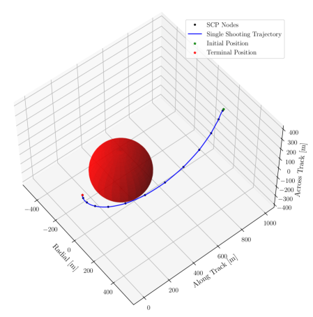
Figure 1: Rendezvous trajectory with spherical keepout

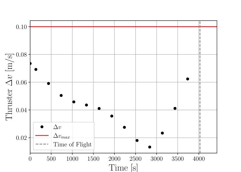
Figure 2: Thruster $\Delta v$

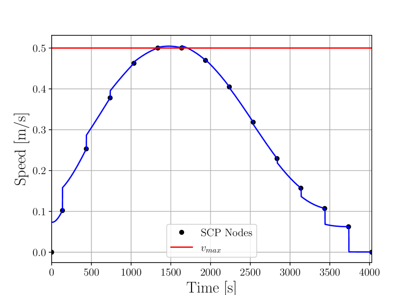
Figure 3: Vehicle speed

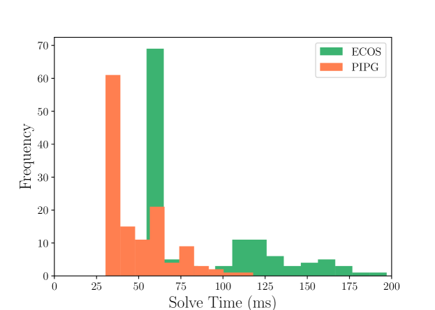
Figure 4: Runtime distribution for 128 solves of the nominal problem

In table 3, we can see that when we use pipg as a subproblem solver we take five more SCP iterations for the trajectory to converge due to the inexact subproblem solves. However, we obtain the same quality solution regardless of which subproblem solver we use as evidenced by the small position and velocity single shooting error. To compare the speeds of ecos and pipg we solved the nominal rendezvous problem 128 times with each subproblem solver and aggregated the total solve times for each SCP solve. The pipg implementation is a naive implementation in Julia which performs memory allocation and solvetime and does not leverage customization, an implementation detail that exploits the structure of the subproblem and eliminates the need for sparse linear algebra, thus making solvetimes faster. Despite this and needing five more SCP iterations to converge, pipg is roughly 1.82 times faster than ecos.

Statistic	ECOS	PIPG
SCP Iterations	13	18
Average Subproblem Solvetime (ms)	90.3	49.5
1$\sigma$ Subproblem Solvetime (ms)	41.1	17.8
Terminal Position Single Shooting Error (m)	0.44	0.45
Terminal Velocity Single Shooting Error (m/s)	$6.4\times 10^{-4}$	$6.4\times 10^{-4}$

Table 3: ecos and pipg solve statistics for nominal rendezvous problem

6.2 Monte Carlo Analysis

In this section, we assess the robustness of pipg as a subproblem solver within SCP to variations in initial conditions. We do this by running a monte carlo with the same problem data and SCP-pipg hyperparameters given in tables 2 and 2 with the exception of the initial position. We sample the initial position from the Gaussian distribution below whose mean, $r_{0}^{nom}$, is the nominal initial position used in the previous section, and whose standard deviation for each position component is 25 meters.

$$r_{0}\sim\mathcal{N}(r_{0}^{nom},25^{2}I_{3})$$ (31)

In our monte carlo, we sampled 128 initial positions and ran SCP to generate trajectories for each of these initial conditions. From Figures 7 and 9 we can see that the single shooting position error is roughly a meter or less regardless of the subproblem solver, which indicates that our solution is dynamically feasible independent of the subproblem solver we use.

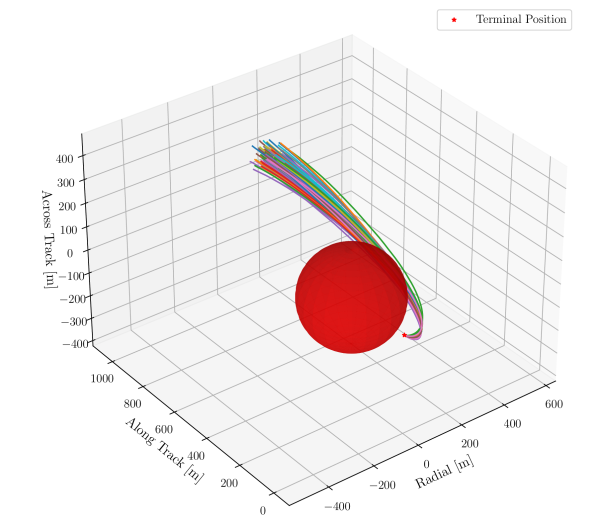
Figure 5: Monte carlo rendezvous trajectories with spherical keepout

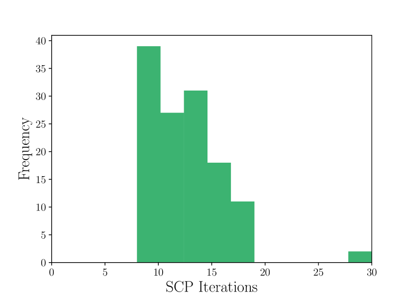
Figure 6: ecos SCP iterations

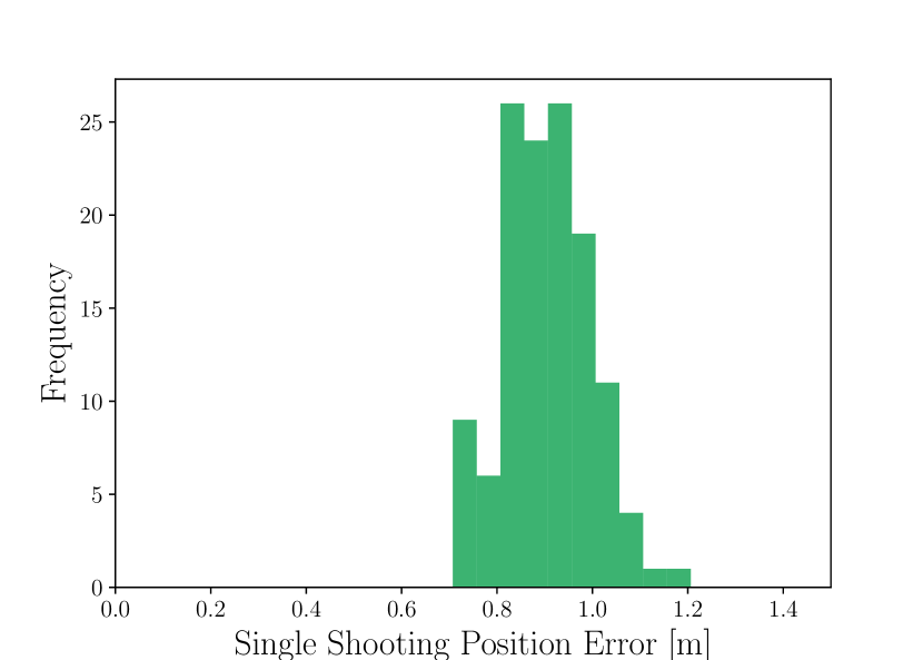
Figure 7: ecos single shooting error

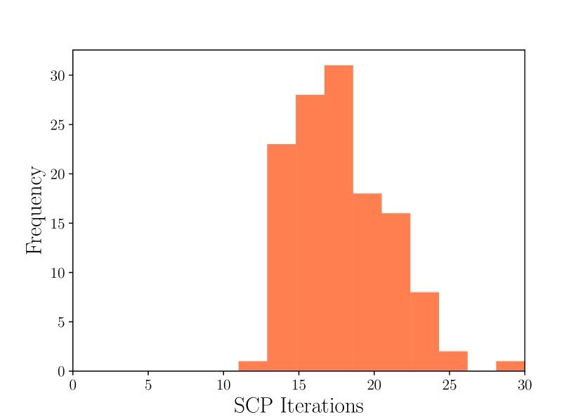
Figure 8: pipg SCP iterations

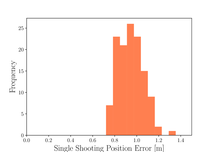
Figure 9: pipg single shooting error

In table 4 we show statistics for the monte carlo simulation. We can see that for both ecos and pipg we have 127 converged trajectories and one trajectory which failed to converge within the 30 SCP iteration cap. From this we can see that although we tuned the pipg hyperparameter, $\omega$ to the nominal rendezvous problem and ran pipg for $100$ iterations for each subproblem, the solver is robust to uncertainty in the initial position. We can also see in the monte carlo that pipg is roughly 1.87 times faster than ecos.

Statistic	ECOS	PIPG
Converged solutions	127/128	127/128
Average SCP Iterations	12.6	17.7
1$\sigma$ SCP Iterations	3.5	3.3
Average Subproblem Solvetime (ms)	91.7	49.1
1$\sigma$ Subproblem Solvetime (ms)	43.0	17.0
Average Terminal Position Single Shooting Error (m)	0.91	0.95
1$\sigma$ Terminal Position Single Shooting Error (m)	0.09	0.11

Table 4: ecos and pipg solve statistics for monte carlo

7 Conclusion

We solved the free final time nonconvex rendezvous problem using sequential convex programming in a factorization-free framework where we used the first-order conic solver pipg to solve the generated sequence of convex subproblems. Although pipg requires tuning of its hyperparameter, $\omega$, for fastest convergence we demonstrated that once tuned for a nominal rendezvous problem, pipg is robust to variations in initial conditions. Given that it is a simpler, more explainable algorithm and we have shown it to be roughly two times faster than ecos, pipg is a good subproblem solver to use within the SCP framework for trajectory optimization for real-time, safety critical. For future work, we plan on developing an adaptive $\omega$ strategy based on balancing primal and dual residuals to remove the need for hyperparameter tuning in pipg.

8 Acknowledgment

The authors would like to thank AJ Berning for discussions on rendezvous problem formulation. We would also like to thank Purnanand Elango, Abhinav Kamath, and Yue Yu for discussions on the efficient implementation of pipg. This research was supported by ONR grant N00014-20-1-2288 and Blue Origin, LLC; Government sponsorship is acknowledged.

References

- [1] G. Chavers, L. Watson-Morgan, M. Smith, N. Suzuki, and T. Polsgrove, “NASA’s Human Landing System: The Strategy for the 2024 Mission and Future Sustainability,” 2020 IEEE Aerospace Conference, 2020, pp. 1–9.
- [2] L. L. Means, “NASA Awards SpaceX Second Contract Option for Artemis Moon Landing,” NASA, 2022.
- [3] C. A. O’Shea, “NASA Selects Blue Origin as Second Artemis Lunar Lander Provider,” NASA, 2023.
- [4] “Vast,” https://www.vastspace.com/. Accessed: 01-14-2024.
- [5] “Axiom Space,” https://www.axiomspace.com/. Accessed: 01-14-2024.
- [6] “Starfish Space,” https://www.starfishspace.com/. Accessed: 01-14-2024.
- [7] D. Malyuta, T. P. Reynolds, M. Szmuk, T. Lew, R. Bonalli, M. Pavone, and B. Açıkmeşe, “Convex Optimization for Trajectory Generation: A Tutorial on Generating Dynamically Feasible Trajectories Reliably and Efficiently,” IEEE Control Systems, Vol. 42, Oct. 2022, pp. 40–113. Free preprint available at https://arxiv.org/abs/2106.09125.
- [8] A. Berning, E. Burnett, and S. Bieniawski, “Chance-Constrained, Drift-Safe Guidance for Spacecraft Rendezvous,” AAS Rocky Mountain Guidance, Navigation and Control Conference, AAS, 2023.
- [9] D. Malyuta, T. Reynolds, M. Szmuk, B. Acikmese, and M. Mesbahi, “Fast Trajectory Optimization via Successive Convexification for Spacecraft Rendezvous with Integer Constraints,” AIAA Scitech 2020 Forum, American Institute of Aeronautics and Astronautics, Jan. 2020.
- [10] D. Malyuta and B. Açıkmeşe, “Fast Homotopy for Spacecraft Rendezvous Trajectory Optimization with Discrete Logic,” Journal of Guidance, Control, and Dynamics, Vol. 46, July 2023, p. 1262–1279.
- [11] A. Domahidi, E. Chu, and S. Boyd, “ECOS: An SOCP solver for embedded systems,” European Control Conference (ECC), 2013, pp. 3071–3076.
- [12] B. O’Donoghue, E. Chu, N. Parikh, and S. Boyd, “Conic Optimization via Operator Splitting and Homogeneous Self-Dual Embedding,” Journal of Optimization Theory and Applications, Vol. 169, June 2016, pp. 1042–1068.
- [13] B. O’Donoghue, “Operator Splitting for a Homogeneous Embedding of the Linear Complementarity Problem,” SIAM Journal on Optimization, Vol. 31, August 2021, pp. 1999–2023.
- [14] B. Stellato, G. Banjac, P. Goulart, A. Bemporad, and S. Boyd, “OSQP: an operator splitting solver for quadratic programs,” Mathematical Programming Computation, Vol. 12, No. 4, 2020, pp. 637–672.
- [15] R. Schwan, Y. Jiang, D. Kuhn, and C. N. Jones, “PIQP: A Proximal Interior-Point Quadratic Programming Solver,” 2023.
- [16] National Aeronautics and Space Administration (NASA) Staff, Verification and Validation of Autonomy Software at NASA. Independently Published, Sept. 2018.
- [17] M. Andersen, J. Dahl, Z. Liu, and L. Vandenberghe, Interior-Point Methods for Large-Scale Cone Programming, p. 55–84. The MIT Press, Sept. 2011.
- [18] Y. Yu, P. Elango, B. Açıkmeşe, and U. Topcu, “Extrapolated Proportional-Integral Projected Gradient Method for Conic Optimization,” IEEE Control Systems Letters, Vol. 7, 2023, pp. 73–78.
- [19] A. G. Kamath, P. Elango, Y. Yu, S. Mceowen, G. M. Chari, J. M. Carson III, and B. Açıkmeşe, “Real-Time Sequential Conic Optimization for Multi-Phase Rocket Landing Guidance,” IFAC-PapersOnLine, Vol. 56, No. 2, 2023, pp. 3118–3125. 22nd IFAC World Congress.
- [20] A. G. Kamath, P. Elango, T. Kim, S. Mceowen, Y. Yu, J. M. Carson III, M. Mesbahi, and B. Açıkmeşe, “Customized Real-Time First-Order Methods for Onboard Dual Quaternion-based 6-DoF Powered-Descent Guidance,” AIAA SciTech 2023 Forum, 2023.
- [21] W. H. Clohessy and R. S. Wiltshire, “Terminal Guidance System for Satellite Rendezvous,” Journal of the Aerospace Sciences, Vol. 27, Sept. 1960, p. 653–658.
- [22] P. Elango, S. Di Cairano, U. Kalabic, and A. Weiss, “Local Eigenmotion Control for Near Rectilinear Halo Orbits,” 2022 American Control Conference (ACC), IEEE, June 2022.
- [23] M. Szmuk, T. P. Reynolds, and B. Açıkmeşe, “Successive Convexification for Real-Time Six-Degree-of-Freedom Powered Descent Guidance with State-Triggered Constraints,” Journal of Guidance, Control, and Dynamics, Vol. 43, No. 8, 2020, pp. 1399–1413.
- [24] G. M. Chari, A. G. Kamath, P. Elango, and B. Acikmese, “Fast Monte Carlo Analysis For 6-DoF Powered-Descent Guidance via GPU-Accelerated Sequential Convex Programming,” AIAA SciTech 2024 Forum, 2024.
- [25] P. Elango, A. G. Kamath, Y. Yu, J. M. Carson III, M. Mesbahi, and B. Açıkmeşe, “A Customized First-Order Solver for Real-Time Powered-Descent Guidance,” AIAA SciTech 2022 Forum, 2022, p. 0951.
- [26] H. H. Bauschke and P. L. Combettes, “Convex Analysis and Monotone Operator Theory in Hilbert Spaces,” CMS Books in Mathematics, 2011.
- [27] S. Boyd and L. Vandenberghe, Convex Optimization. Cambridge University Press, Mar. 2004.
- [28] D. Dueri, Y. Mao, Z. Mian, J. Ding, and B. Açikmeşe, “Trajectory optimization with inter-sample obstacle avoidance via successive convexification,” 2017 IEEE 56th Annual Conference on Decision and Control (CDC), 2017, pp. 1150–1156.