On the minimax robustness against correlation and heteroscedasticity of ordinary least squares among generalized least squares estimators of regression

Abstract

We present a result according to which certain functions of covariance matrices are maximized at scalar multiples of the identity matrix. In a statistical context in which such functions measure loss, this says that the least favourable form of dependence is in fact independence, so that a procedure optimal for i.i.d. data can be minimax. In particular, the ordinary least squares (ols) estimate of regression is minimax, in the class of generalized least squares estimates, when the maximum is taken over certain classes of error covariance structures and the loss function possesses a natural monotonicity property. An implication is that it can be safe to ignore such departures – whose precise form is typically unknown – from the usual assumption of i.i.d. errors. We then consider regression models in which the response function is possibly misspecified, and show that, depending on the design, ols can fail to be minimax. We argue that the gains from a minimax estimate are however often outweighed by the simplicity of ols. We go on to investigate the interplay between minimax precision matrices and minimax designs. We find that the design has by far the major influence on efficiency and that, when the two are combined, ols is generally at least ‘almost’ minimax, and often exactly so.

1 Introduction and summary

When carrying out a study, whether observational or designed, calling for a regression analysis the investigator may be faced with questions regarding possible correlations or heteroscedasticity within the data. If there are such departures from the assumptions underlying the use of the ordinary least squares (ols) estimates of the regression parameters, then the use of generalized least squares (gls) might be called for. In its pure form, as envisioned by Aitken (1935), this calls for the use of the inverse of the covariance matrix $C$, i.e. the precision matrix, of the random errors. This is inconvenient, since $C$ is rarely known and, even if there is some prior knowledge of its structure, before the study is carried out there are no data from which accurate estimates of its elements might be made. If a consistent estimate $\hat{C}^{-1}$ of the precision matrix does exist, then one can employ ‘feasible generalized least squares’ estimation - see e.g. Fomby, Johnson & Hill (1984). Otherwise a positive definite ‘pseudo precision’ matrix $P$ might be employed. With data $y$ and design matrix $X$ this leads to the estimate

$$\hat{\theta}_{\text{{gls}}}=\left(X^{\prime}PX\right)^{-1}X^{\prime}Py.$$ (1)

In Wiens (2024) a similar problem was addressed, pertaining to designed experiments whose data are to be analyzed by ols. A lemma, restated below as Lemma 1, was used to show that certain commonly employed loss functions, taking covariance matrices as their arguments and increasing with respect to the Loewner ordering by positive semidefiniteness, are maximized at scalar multiples of the identity matrix. This has the somewhat surprising statistical interpretation that the least favourable form of dependence is in fact independence. The lemma was used to show that the assumption of independent and homoscedastic errors at the design stage of an experiment is in fact a minimax strategy, within broad classes of alternate covariance structures.

In this article we study the implications of the lemma in the problem of choosing between ols and gls. We first show that, when the form of the regression response is accurately modelled, then it can be safe – in a minimax sense – to ignore possible departures from independence and homoscedasticity, varying over certain large classes of such departures. This is because the common functions measuring the loss incurred by gls, when the covariance matrix of the errors is $C$, are maximized when $C$ is a multiple of the identity matrix. But in that case the best gls estimate is in fact ols, i.e. ols is a minimax procedure.

We then consider the case of misspecified regression models, in which bias becomes a component of the integrated mean squared prediction error (imspe). The imspe is maximized over $C$ and over the departures from the fitted linear model. We show that, if a gls with (pseudo) precision matrix $P$ is employed, then the variance component of this maximum continues to be minimized by $P=I$, i.e. by ols, but the bias generally does not and, depending upon the design, ols can fail to be a minimax procedure. This is in contrast to the findings in Wiens (2024), where incorrectly assuming that $C\propto I$ at the design stage did not affect the bias, and so designing for independence remained a minimax procedure.

We present an algorithm allowing us to determine the minimax choice of $P$ numerically, and study this for a large number of designs. It turns out that, if a sensible design is chosen, then $P=I$ is ‘almost’ a minimax choice. When a minimax design – minimizing the maximum imspe over the design as well as over $P$ – is also chosen, then $P=I$ is often exactly minimax. We conclude that, for Loewner-increasing loss functions, and for covariance matrices $C$ varying over the classes covered by Lemma 1, the simplicity of ols makes it a safe and attractive alternative to gls.

The computations for this article were carried out in matlab; the code is available on the author’s personal website.

2 A useful lemma

Suppose that $\left\|\cdot\right\|_{M}$ is a matrix norm, induced by the vector norm $\left\|\cdot\right\|_{V}$, i.e.

$$\left\|C\right\|_{M}=\sup_{\left\|x\right\|_{V}\text{ }=1}\left\|Cx\right\|_{V}.$$

We use the subscript ‘$M$’ when referring to an arbitrary matrix norm, but adopt special notation in the following cases:

(i) For the Euclidean norm $\left\|x\right\|_{V}=(x^{\prime}x)^{1/2}$, the matrix norm is denoted $\left\|C\right\|_{E}$ and is the spectral radius, i.e. the root of the maximum eigenvalue of $C^{\prime}C$. This is the maximum eigenvalue of $C$ if $C$ is a covariance matrix, i.e. is symmetric and positive semidefinite.

(ii) For the sup norm $\left\|x\right\|_{V}=\max_{i}\left|x_{i}\right|$, the matrix norm $\left\|C\right\|_{\infty}$ is $\max_{i}\sum_{j}\left|c_{ij}\right|$, the maximum absolute row sum.

(iii) For the 1-norm $\left\|x\right\|_{V}=\sum_{i}\left|x_{i}\right|$, the matrix norm $\left\|C\right\|_{1}$ is $\max_{j}\sum_{i}\left|c_{ij}\right|$, the maximum absolute column sum. For symmetric matrices, $\left\|C\right\|_{1}=\left\|C\right\|_{\infty}$.

Now suppose that the loss function in a statistical problem is $\mathcal{L}\left(C\right)$, where $C$ is an $n\times n$ covariance matrix and $\mathcal{L}\left(\mathbf{\cdot}\right)$ is non-decreasing in the Loewner ordering:

$$A\preceq B\Rightarrow\mathcal{L}\left(A\right)\leq\mathcal{L}\left(B\right).$$

Here $A\preceq B$ means that $B-A\succeq 0$, i.e. is positive semidefinite.

The following lemma is established in Wiens (2024).

Lemma 1.

For $\eta^{2}>0$, covariance matrix $C$ and induced norm $\left\|C\right\|_{M}$, define

$$\mathcal{C}_{M}=\left\{C\left|{}\right.C\succeq 0\text{ and }\left\|C\right\|_{M}\leq\eta^{2}\right\}.$$ (2)

For the norm $\left\|\mathbf{\cdot}\right\|_{E}$ an equivalent definition is

$$\mathcal{C}_{E}=\left\{C\left|{}\right.0\preceq C\preceq\eta^{2}I_{n}\right\}.$$

Then:

(i) In any such class $\mathcal{C}_{M}$, $\max_{\mathcal{C}_{M}}\mathcal{L}\left(C\right)=\mathcal{L}\left(\eta^{2}I_{n}\right)$.

(ii) If $\mathcal{C}^{\prime}$ $\mathcal{\subseteq C}_{M}$ and $\eta^{2}I_{n}\in\mathcal{C}^{\prime}$, then $\max_{\mathcal{C}^{\prime}}\mathcal{L}\left(C\right)=\mathcal{L}\left(\eta^{2}I_{n}\right)$.

A consequence of (i) of this lemma is that if one is carrying out a statistical procedure with loss function $\mathcal{L}\left(C\right)$, then a version of the procedure which minimizes $\mathcal{L}\left(\eta^{2}I_{n}\right)$ is minimax as $C$ varies over $\mathcal{C}_{M}$. The procedures discussed in this article do not depend on the particular value of $\eta^{2}$ – its only role is to ensure that $\mathcal{C}_{M}$ is large enough to contain the departures of interest.

3 Generalized least squares regression estimates when the response is correctly specified

Consider the linear model

$$y=X\theta+\varepsilon$$ (3)

for $X_{n\times p}$ of rank $p$. Suppose that the random errors $\varepsilon$ have covariance matrix $C\in\mathcal{C}_{M}$. If $C$ is known then the ‘best linear unbiased estimate’ is $\hat{\theta}_{\text{{blue}}}=$ $\left(X^{\prime}C^{-1}X\right)^{-1}X^{\prime}C^{-1}y$. In the more common case that the covariances are at best only vaguely known, an attractive possibility is to use the generalized least squares estimate (1) for a given positive definite (pseudo) precision matrix $P$. If $P=C^{-1}$ then the blue is returned. A diagonal $P$ gives ‘weighted least squares’ (wls). For brevity we drop the ‘pseudo’ and call $P$ a precision matrix. Since $\hat{\theta}_{\text{{gls}}}$ is invariant under multiplication of $P$ by a scalar, we assume throughout that

$$tr\left(P\right)=n.$$ (4)

The covariance matrix of $\hat{\theta}_{\text{{gls}}}$ is

$$\text{{cov}}\left(\hat{\theta}_{\text{{gls}}}\left|{}\right.C,P\right)=\left(X^{\prime}PX\right)^{-1}X^{\prime}PCPX\left(X^{\prime}PX\right)^{-1}.$$

Viewed as a function of $C$ this is non-decreasing in the Loewner ordering, so that if a function $\Phi$ is non-decreasing in this ordering, then

$$\mathcal{L}\left(C\left|{}\right.P\right)=\Phi\{\text{{cov}}(\hat{\theta}_{\text{{gls}}}\mid C,P)\}$$

is also non-decreasing and the conclusions of the lemma hold:

$$\max_{\mathcal{C}_{M}}\mathcal{L}\left(C\left|{}\right.P\right)=\mathcal{L}\left(\eta^{2}I_{n}\left|{}\right.P\right)=\Phi\left\{\eta^{2}\left(X^{\prime}PX\right)^{-1}XP^{2}X\left(X^{\prime}PX\right)^{-1}\right\}.$$

But this last expression is minimized by $P=I_{n}$, i.e. by the ols estimate $\hat{\theta}_{\text{{ols}}}=\left(X^{\prime}X\right)^{-1}X^{\prime}y$, with minimum value

$$\max_{\mathcal{C}_{M}}\mathcal{L}\left(C\left|{}\right.I_{n}\right)=\Phi\left\{\eta^{2}\left(X^{\prime}X\right)^{-1}\right\}.$$

This follows from the monotonicity of $\Phi$ and the inequality

$$\eta^{2}\left(X^{\prime}PX\right)^{-1}X^{\prime}P^{2}X\left(X^{\prime}PX\right)^{-1}-\eta^{2}\left(X^{\prime}X\right)^{-1}$$

$$= \eta^{2}\left(X^{\prime}PX\right)^{-1}X^{\prime}P\left\{I_{n}-X\left(X^{\prime}X\right)^{-1}X^{\prime}\right\}PX\left(X^{\prime}PX\right)^{-1}$$

$$\succeq 0,$$

which uses the fact that $I_{n}-X\left(X^{\prime}X\right)^{-1}X^{\prime}$ is idempotent, hence positive semidefinite.

It is well-known that if $0\preceq\Sigma_{1}\preceq\Sigma_{2}$ then the $i$th largest eigenvalue $\lambda_{i}$ of $\Sigma_{2}$ dominates that of $\Sigma_{1}$, for all $i$. It follows that $\Phi$ is non-decreasing in the Loewner ordering in the cases:

(i) $\Phi\left(\Sigma\right)=tr\left(\Sigma\right)=\sum_{i}\lambda_{i}\left(\Sigma\right)$;

(ii) $\Phi\left(\Sigma\right)=det\left(\Sigma\right)=\prod_{i}\lambda_{i}\left(\Sigma\right)$;

(iii) $\Phi\left(\Sigma\right)=\max_{i}\lambda_{i}\left(\Sigma\right)$;

(iv) $\Phi\left(\Sigma\right)=tr\left(K\Sigma\right)$ for $K\succeq 0$.

Thus if loss is measured in any of these ways and $C\in\mathcal{C}_{M}$ then $\hat{\theta}_{\text{{ols}}}$ is minimax for $\mathcal{C}_{M}$ in the class of gls estimates.

In each of the following examples, we posit a particular covariance structure for $C$, a norm $\left\|C\right\|_{M}$ , a bound $\eta^{2}$ and a class $\mathcal{C}^{\prime}$ for which $C\in\mathcal{C}^{\prime}\subseteq\mathcal{C}_{M}$. In each case $\eta^{2}I_{n}\in\mathcal{C}^{\prime}$, so that statement (ii) of the lemma applies and $\hat{\theta}_{\text{{ols}}}$ is minimax for $\mathcal{C}^{\prime}$ (and for all of $\mathcal{C}_{M}$ as well) and with respect to any of the criteria (i) – (iv).

Example 1: Independent, heteroscedastic errors. Suppose that $C=diag(\sigma_{1}^{2},...,\sigma_{n}^{2})$. Then the discussion above applies if $\mathcal{C}^{\prime}$ is the subclass of diagonal members of $\mathcal{C}_{E}$ for $\eta^{2}=\max_{i}\sigma_{i}^{2}$.

Example 2: Equicorrelated errors. Suppose that the researcher fears that the observations are possibly weakly correlated, and so considers $C=\sigma^{2}\left(\left(1-\rho\right)I_{n}+\rho 1_{n}1_{n}^{\prime}\right)$, with $\left|\rho\right|\leq\rho_{\max}$. If $\rho$ $\geq 0$ then $\left\|C\right\|_{1}=\left\|C\right\|_{\infty}=\left\|C\right\|_{E}=\leavevmode\nobreak\ \sigma^{2}\left\{1+\left(n-1\right)\left|\rho\right|\right\}$, and we take $\eta^{2}=\sigma^{2}\left\{1+\left(n-1\right)\rho_{\max}\right\}$. If $\mathcal{C}^{\prime}$ is the subclass of $\mathcal{C}_{1}$ or $\mathcal{C}_{\infty}$ or $\mathcal{C}_{E}$ defined by the equicorrelation structure, then minimaxity of $\hat{\theta}_{\text{{ols}}}$ for any of these classes follows. If $\rho<0$ then this continues to hold for $\mathcal{C}_{1}=\mathcal{C}_{\infty}$, and for $\mathcal{C}_{E}$ if $\eta^{2}=\sigma^{2}\left(1+\rho_{\max}\right)$.

Example 3: ma${\small(1)}$ errors. Assume first that the random errors are homoscedastic but are possibly serially correlated, following an ma${\small(1)}$ model with corr$(\varepsilon_{i},\varepsilon_{j})=\rho I\left(\left|i-j\right|=1\right)$ and with $\left|\rho\right|\leq\rho_{\max}$. Then $\left\|C\right\|_{1}=\left\|C\right\|_{\infty}\leq\sigma^{2}\left(1+2\rho_{\max}\right)=\eta^{2}$, and in the discussion above we may take $\mathcal{C}^{\prime}$ to be the subclass – containing $\eta^{2}I_{n}$ – defined by $c_{ij}=0$ if $\left|i-j\right|>1$. If the errors are instead heteroscedastic, then $\sigma^{2}$ is replaced by $\max_{i}\sigma_{i}^{2}$.

Example 4: ar${\small(1)}$ errors. It is known – see for instance Trench (1999, p. 182) – that the eigenvalues of an ar${\small(1)}$ autocorrelation matrix with autocorrelation parameter $\rho$ are bounded, and that the maximum eigenvalue $\lambda\left(\rho\right)$ has $\lambda^{\ast}=$ $\max_{\rho}\lambda\left(\rho\right)>\lambda\left(0\right)=1$. Then, again under homoscedasticity, the covariance matrix $C$ has $\left\|C\right\|_{E}\leq\sigma^{2}\lambda^{\ast}=\eta^{2}$, and the discussion above applies when $\mathcal{C}^{\prime}$ is the subclass defined by the autocorrelation structure.

3.1 Inference from GLS estimates when $C=$ $\sigma^{2}I_{n}$

In the next section we consider biased regression models, and investigate the performance of the gls estimate (1) with $P\neq I_{n}$ when in fact $C$ is a multiple $\sigma^{2}$ of the identity matrix. A caveat to the use of this estimate in correctly specified models (3) is given by the following result. It was established in Wiens (2000) for wls estimates, but holds for gls estimates as well.

Theorem 1.

Suppose that data $y_{n\times 1}$ obey the linear model (3) with $C=$ $\sigma^{2}I_{n}$ and that a gls estimate (1), with $P\neq I_{n}$, is employed. Let $H:n\times n$ be the projector onto the column space of $(X\vdots PX):n\times 2p$. Then an unbiased estimate of $\sigma^{2}$ is

$$S^{2}=\left\|\left(I_{n}-H\right)y\right\|^{2}/\left(n-rk\left(H\right)\right).$$

The vector $\left(I_{n}-H\right)y$ is uncorrelated with $\hat{\theta}_{\text{{gls}}}$. If the errors are normally distributed, then $S^{2}\sim\sigma^{2}\chi_{n-rk\left(H\right)}^{2}$, independently of $\hat{\theta}_{\text{{gls}}}$.

The projector $H$ will typically have rank $2p$ when $P\neq I_{n}$, and so $p$ degrees of freedom are lost in the estimation of $\sigma^{2}$ and subsequent normal-theory inferences.

4 Minimax precision matrices in misspecified response models

Working in finite design spaces $\chi=\left\{x_{i}\right\}_{i=1}^{N}\subset\mathbb{R}^{d}$, and with $p$-dimensional regressors $f\left(x\right)$, Wiens (2018) studied design problems for possibly misspecified regression models

$$Y\left(x\right)=f^{\prime}\left(x\right)\theta+\psi\left(x\right)+\varepsilon,$$

with the unknown contaminant $\psi$ ranging over a class $\Psi$ and satisfying, for identifiability of $\theta$, the orthogonality condition

$$\sum_{x\in\chi}f\left(x\right)\psi\left(x\right)=0_{p\times 1},$$ (5)

as well as a bound

$$\sum_{x\in\chi}\psi^{2}\left(x\right)\leq\tau^{2}.$$ (6)

For designs $\xi$ placing mass $\xi_{i}$ on $x_{i}\in\chi$, he took $\hat{\theta}=\hat{\theta}_{\text{{ols}}}$, loss function imspe:

$$\mathcal{I}\left(\psi,\xi\right)=\sum_{x\in\chi}E[f^{\prime}\left(x\right)\hat{\theta}-E\{Y\left(x\right)\}]^{2},$$

and found designs minimizing the maximum, over $\psi$, of $\mathcal{I}\left(\psi,\xi\right)$.

In Wiens (2018) the random errors $\varepsilon_{i}$ were assumed to be i.i.d.; now suppose that they instead have covariance matrix $C\in\mathcal{C}_{M}$ and take $\hat{\theta}=\hat{\theta}_{\text{{gls}}}$ with precision matrix $P$. Using (5), and emphasizing the dependence on $C$ and $P$, $\mathcal{I}\left(\psi,\xi\right)$ decomposes as

$$\mathcal{I}\left(\psi,\xi\left|{}\right.C,P\right)=\sum_{x\in\chi}f^{\prime}\left(x\right)\text{{cov}}\left(\hat{\theta}\left|{}\right.C,P\right))f\left(x\right)+\sum_{x\in\chi}f^{\prime}\left(x\right)b_{\psi,P}b_{\psi,P}^{\prime}f\left(x\right)+\sum_{x\in\chi}\psi^{2}\left(x\right).$$ (7)

Here $b_{\psi,P}=E(\hat{\theta})-\theta$ is the bias. Denote by $\psi_{X}$ the $n\times 1$ vector consisting of the values of $\psi$ corresponding to the rows of $X$, so that $b_{\psi,P}=\left(X^{\prime}PX\right)^{-1}X^{\prime}P\psi_{X}$.

To express these quantities in terms of the design, define a set of $n\times N$ indicator matrices

$$\mathcal{J}=\left\{J\in\left\{0,1\right\}^{n\times N}\left|{}\right.J^{\prime}J\text{ is diagonal with trace }n\right\}.$$

There is a one-one correspondence between $\mathcal{J}$ and the set of $n$-point designs on $\chi$. Given $J$, with $J^{\prime}J=diag\left(n_{1},...,n_{N}\right)$, the $j$th column of $J$ contains $n_{j}$ ones, specifying the number of occurrences of $x_{j}$ in a design, which thus has design vector $\xi=n^{-1}J^{\prime}1_{n}=\left(n_{1}/n,...,n_{N}/n\right)^{\prime}$. Conversely, a design determines $J$ by $J_{ij}=$ $I\left(\text{the }i\text{th row of }X\text{ is }f^{\prime}\left(x_{j}\right)\right)$.

Define $F_{N\times p}$ to be the matrix with rows $\left\{f^{\prime}\left(x_{i}\right)\right\}_{i=1}^{N}$. Then $X=JF$ and, correspondingly, $\psi_{X}=J\bar{\psi}$ for $\bar{\psi}=\left(\psi\left(x_{1}\right),...,\psi\left(x_{N}\right)\right)^{\prime}$.

The proof of the following theorem is in the appendix.

Theorem 2.

For $\eta$ as at (2) and $\tau$ as at (6), define $\nu=\tau^{2}/\left(\tau^{2}+\eta^{2}\right)$; this is the relative importance to the designer of errors due to bias rather than to variation. Then for a design $\xi$ and precision matrix $P$, the maximum of $\mathcal{I}\left(\psi,\xi\left|{}\right.C,P\right)$ as $C$ varies over $\mathcal{C}_{M}$ and $\psi$ varies over $\Psi$ is $\left(\tau^{2}+\eta^{2}\right)\times$

$$\mathcal{I}_{\nu}\left(\xi,P\right)=\left(1-\nu\right)\mathcal{I}_{0}\left(\xi,P\right)+\nu\mathcal{I}_{1}\left(\xi,P\right),$$ (8)

where

$$\mathcal{I}_{0}\left(\xi,P\right) = tr\left\{\left(Q^{\prime}UQ\right)^{-1}\left(Q^{\prime}VQ\right)\left(Q^{\prime}UQ\right)^{-1}\right\},$$

$$\mathcal{I}_{1}\left(\xi,P\right) = ch_{\max}\left\{\left(Q^{\prime}UQ\right)^{-1}Q^{\prime}U^{2}Q\left(Q^{\prime}UQ\right)^{-1}\right\},$$

$$U_{N\times N} = J^{\prime}PJ\text{\ and }V_{N\times N}=J^{\prime}P^{2}J.$$

Here the columns of $Q_{N\times p}$ form an orthogonal basis for the column space ${col}\left(F\right)$, $J$ is the indicator matrix of the design $\xi$, and $ch_{\max}$ denotes the maximum eigenvalue of a matrix.

In (8), var $=$ $\mathcal{I}_{0}$ and bias $=$ $\mathcal{I}_{1}$ are the components of the imspe due to variation and to bias, respectively. That $\mathcal{I}_{0}\left(\xi,P\right)$ is minimized by $P=I_{n}$ for any design was established in §3. If ols is to be a minimax procedure for a particular design, then for each $\nu\in(0,1]$ any increase in bias must be outweighed by a proportional decrease in var. We shall present numerical evidence that for many designs this is not the case, and then ols is not minimax.

To find $P$ minimizing (8) we note that any positive definite matrix can be represented as $P=L^{\prime}L$, for a lower triangular $L$. We thus express $\mathcal{I}_{\nu}\left(\xi,L^{\prime}L\right)$ as a function of the vector $l_{n\left(n+1\right)/2\times 1}$ consisting of the elements in the lower triangle of $L$, and minimize over $l$ using a nonlinear constrained minimizer. The constraint – recall (4) – is that $l^{\prime}l=n$.

Of course we cannot guarantee that these methods yield an absolute minimum, but the numerical evidence is compelling. In any event, the numerical results give a negative answer to the question of whether or not ols is necessarily minimax for any design – the minimizing $P$ is often, but not always, the identity.

To assess these precision matrices we carried out a simulation study. We set the design space to be $\chi=\left\{-1=x_{1}<\cdot\cdot\cdot<x_{N}=1\right\}$, with the $x_{i}$ equally spaced. We chose regressors $f\left(x\right)=\left(1,x\right)^{\prime}$, $\left(1,x,x^{2}\right)^{\prime}$ or $\left(1,x,x^{2},x^{3}\right)^{\prime}$, corresponding to linear, quadratic, or cubic regression. For various values of $n$ and $N$ we first randomly generated probability distributions $\left(p_{1},p_{2},..,p_{N}\right)$ and then generated a multinomial$\left(n;p_{1},p_{2},..,p_{N}\right)$ vector; this is $n\xi$. For each such design we computed the minimizing $P$, and both components of the minimized value of $\mathcal{I}_{\nu}\left(\xi,P\right)$. This was done for $\nu=.5,1$. We took $n$ equal to five times the number of regression parameters. Denote by $P_{\nu}$ the minimizing $P$. Of course $P_{0}=I_{n}$. In each case we compared three quantities:

$$T_{1} = 100\frac{\left(\mathcal{I}_{\nu}\left(\xi,P_{0}\right)-\mathcal{I}_{\nu}\left(\xi,P_{\nu}\right)\right)}{\mathcal{I}_{\nu}\left(\xi,P_{0}\right)}\text{, the percent reduction in }\mathcal{I}_{\nu}\text{ achieved by }P_{\nu};$$

$$T_{2} = 100\frac{\left(\mathcal{I}_{0}\left(\xi,P_{\nu}\right)-\mathcal{I}_{0}\left(\xi,P_{0}\right)\right)}{\mathcal{I}_{0}\left(\xi,P_{0}\right)}\text{, the percent increase, relative to {ols}, in {var};}$$

$$T_{3} = 100\frac{\left(\mathcal{I}_{1}\left(\xi,P_{0}\right)-\mathcal{I}_{1}\left(\xi,P_{\nu}\right)\right)}{\mathcal{I}_{1}\left(\xi,P_{0}\right)}\text{, the percent decrease, relative to {ols}, in {bias}.}$$

The means, and standard errors based on 100 runs, of these performance measures using these ‘multinomial’ designs are given in Table 1. When $\nu=1$ the percent reduction in the bias, i.e. in $T_{3}$, can be significant, but is accompanied by an often sizeable increase in the variance ($T_{2}$). When $\nu=.5$ the reduction in $T_{1}$ is typically quite modest.

Table 1.  Minimax precision matrices; multinomial designs:
means of performance measures $\pm$ $1$ standard error.
Response	$N$	$\nu$		$\mathcal{I}_{\nu}\left(\xi,I_{n}\right)$	$\mathcal{I}_{\nu}\left(\xi,P_{\nu}\right)$	$T_{1}\left(\%\right)$	$T_{2}\left(\%\right)$	$T_{3}\left(\%\right)$
	$11$	$.5$		$2.83\pm.10$	$2.71\pm.09$	$4.16\pm.30$	$2.91\pm.21$	$10.58\pm.69$
linear	$11$	$1$		$3.97\pm.37$	$3.50\pm.34$	$12.46\pm.85$	$9.83\pm.83$	$12.46\pm.85$
$n=10$	$51$	$.5$		$10.43\pm.34$	$10.32\pm.34$	$1.02\pm.12$	$.74\pm.09$	$3.12\pm.34$
	$51$	$1$		$10.28\pm.74$	$9.76\pm.71$	$4.58\pm.49$	$3.20\pm.37$	$4.58\pm.49$
	$11$	$.5$		$4.51\pm.59$	$4.29\pm.56$	$4.66\pm.34$	$3.14\pm.23$	$11.91\pm.79$
quadratic	$11$	$1$		$4.18\pm.47$	$3.62\pm.42$	$13.43\pm.71$	$8.91\pm.58$	$13.43\pm.71$
$n=15$	$51$	$.5$		$12.84\pm.85$	$12.63\pm.83$	$1.57\pm.15$	$1.00\pm.10$	$5.16\pm.45$
	$51$	$1$		$10.45\pm 1.00$	$9.82\pm.93$	$5.98\pm.52$	$3.40\pm.36$	$5.98\pm.52$
	$11$	$.5$		$5.44\pm.62$	$5.19\pm.60$	$4.61\pm.31$	$2.89\pm.19$	$11.97\pm.81$
cubic	$11$	$1$		$12.19\pm 2.47$	$11.054\pm 2.30$	$12.43\pm.88$	$8.46\pm.71$	$12.43\pm.88$
$n=20$	$51$	$.5$		$12.22\pm 1.11$	$12.03\pm 1.09$	$1.52\pm.12$	$.89\pm.07$	$5.62\pm.40$
	$51$	$1$		$19.97\pm 4.20$	$18.64\pm 3.89$	$6.19\pm.43$	$3.13\pm.29$	$6.19\pm.43$

Table 2.  Minimax precision matrices; symmetrized designs:
means of performance measures $\pm$ $1$ standard error.
Response	$N$	$\nu$		$\mathcal{I}_{\nu}\left(\xi,I_{n}\right)$	$\mathcal{I}_{\nu}\left(\xi,P_{\nu}\right)$	$T_{1}\left(\%\right)$	$T_{2}\left(\%\right)$	$T_{3}\left(\%\right)$
	$11$	$.5$		$2.06\pm.05$	$2.00\pm.04$	$2.50\pm.30$	$1.50\pm.16$	$7.36\pm.76$
linear	$11$	$1$		$1.84\pm.11$	$1.67\pm.11$	$8.33\pm.79$	$4.30\pm.38$	$8.33\pm.79$
$n=10$	$51$	$.5$		$9.33\pm.33$	$9.29\pm.33$	$.43\pm.08$	$.26\pm.05$	$1.50\pm.28$
	$51$	$1$		$7.39\pm.42$	$7.28\pm.43$	$1.84\pm.32$	$.72\pm.13$	$1.84\pm.32$
	$11$	$.5$		$2.95\pm.77$	$2.87\pm.75$	$2.59\pm.21$	$1.71\pm.11$	$9.25\pm.62$
quadratic	$11$	$1$		$1.77\pm.17$	$1.53\pm.16$	$14.31\pm.82$	$8.26\pm.48$	$14.31\pm.82$
$n=15$	$51$	$.5$		$9.78\pm.63$	$9.76\pm.63$	$.26\pm.11$	$.16\pm.07$	$.85\pm.33$
	$51$	$1$		$6.34\pm.49$	$6.27\pm.48$	$.90\pm.37$	$.42\pm.19$	$.90\pm.37$
	$11$	$.5$		$2.36\pm.17$	$2.27\pm.16$	$3.59\pm.29$	$2.05\pm.15$	$12.40\pm.81$
cubic	$11$	$1$		$2.06\pm.20$	$1.71\pm.19$	$18.60\pm 1.21$	$10.99\pm.69$	$18.60\pm 1.21$
$n=20$	$51$	$.5$		$10.88\pm 1.45$	$10.84\pm 1.44$	$.38\pm.06$	$.21\pm.04$	$1.68\pm.29$
	$51$	$1$		$6.34\pm.98$	$6.23\pm.98$	$2.18\pm.39$	$.79\pm.15$	$2.18\pm.39$

These multinomial designs, mimicking those which might arise in observational studies, are not required to be symmetric. We re-ran the simulations after symmetrizing the designs by averaging them with their reflections across $x=0$ and then applying a rounding mechanism which preserved symmetry. The resulting designs gave substantially reduced losses both for $P=I_{n}$ (ols) and $P=P_{\nu}$ (gls). The differences between the means of $\mathcal{I}_{\nu}\left(\xi,I_{n}\right)$ and $\mathcal{I}_{\nu}\left(\xi,P_{\nu}\right)$ were generally statistically insignificant, and the values of $T_{1}$, $T_{2}$ and $T_{3}$ showed only very modest benefits to gls. See Table 2.

A practitioner might understandably conclude that, even though $P_{\nu}$ is minimax, its benefits are outweighed by the computational complexity of its implementation. This is bolstered by Theorem 1, which continues to hold with the modification that $S^{2}$ now follows a scaled non-central $\chi^{2}$ distribution, with a non-centrality parameter depending on $\psi_{X}^{\prime}\left(I_{n}-H\right)\psi_{X}$.

5 Minimax precision matrices and minimax designs

Table 3.  Minimax designs and precision matrices:
performance measures ($T_{1}=T_{2}=T_{3}=0$ if $P_{\nu}=I_{n}$).
Response	$N$	$\nu$		$\mathcal{I}_{\nu}\left(\xi,I_{n}\right)$	$\mathcal{I}_{\nu}\left(\xi,P_{\nu}\right)$	$T_{1}(\%)$	$T_{2}(\%)$	$T_{3}(\%)$
	$11$	$.5$		$1.60$	$1.60$	$0$	$0$	$0$
linear	$11$	$1$		$1.10$	$1.10$	$0$	$0$	$0$
$n=10$	$51$	$.5$		$6.14$	$6.14$	$0$	$0$	$0$
	$51$	$1$		$5.10$	$5.10$	$0$	$0$	$0$
	$11$	$.5$		$1.61$	$1.53$	$4.67$	$2.81$	$16.06$
quadratic	$11$	$1$		$1.12$	$1.00$	$10.84$	$10.78$	$10.84$
$n=15$	$51$	$.5$		$5.80$	$5.80$	$0$	$0$	$0$
	$51$	$1$		$3.40$	$3.40$	$0$	$0$	$0$
	$11$	$.5$		$1.55$	$1.53$	$1.46$	$1.13$	$6.04$
cubic	$11$	$1$		$1.12$	$1.00$	$11.03$	$4.84$	$11.03$
$n=20$	$51$	$.5$		$5.56$	$5.56$	$0$	$0$	$0$
	$51$	$1$		$2.55$	$2.55$	$0$	$0$	$0$

We investigated the interplay between minimax precision matrices and minimax designs. To this end (8) was minimized over both $\xi$ and $P$. To minimize over $\xi$ we employed particle swarm optimization (Kennedy and Eberhart 1995). The algorithm searches over continuous designs $\xi$, and so each such design to be evaluated was first rounded so that $n\xi$ had integer values. Then $J$, and the corresponding minimax precision matrix $P_{\nu}=P_{\nu}\left(J\right)$ were computed and the loss returned. The final output is an optimal pair $\left\{J_{\nu},P_{\nu}\right\}$. Using a genetic algorithm yielded the same results but was many times slower.

The results, using the same parameters as in Tables 1 and 2, are shown in Table 3. We note that in all cases the use of the minimax design gave significantly smaller losses, both using ols and gls. In eight of the twelve cases studied it turned out that the choice $P=I_{n}$ was in fact minimax; in the remaining cases minimax precision resulted in only a marginal improvement. Of the two factors – $\xi$ and $P$ – explaining the decrease in $\mathcal{I}_{\nu}$, the design is by far the greater contributor.

See Figure 1 for some representative plots of the minimax designs for a cubic response. These reflect several common features of robust designs. One is that the designs using $\nu=1$, i.e. aimed at minimization of the bias alone, tend to be more uniform than those using $\nu=.5$. This reflects the fact – following from (5) – that if a uniform design on all of $\chi$ could be implemented, then the bias using ols would vanish. As well, when the design space is sufficiently rich as to allow for clusters of nearby design points to replace replicates, then this tends to take place. See Wiens (2023), Fang and Wiens (2000) and Heo et al. (2001) for examples and discussions. Such clusters form near the support points of the classically I-optimal designs, minimizing variance alone.

In their study of random design strategies on continuous design spaces, Waite and Woods (2022) also recommend designs with clusters chosen near the I-optimal design points. See Studden (1977) who showed that the I-optimal design for cubic regression places masses $.1545$, $.3455$ at each of $\pm 1$, $\pm.477$ - a situation approximated by the design in (c) of Figure 1, whose clusters around these points account for masses of $.15$ and $.35$ each.

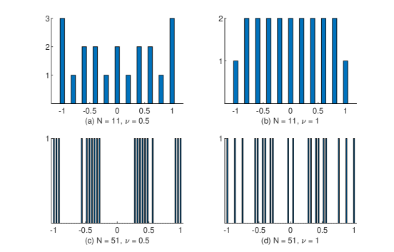
Figure 1: Minimax design frequencies for a cubic model; $n=20$.

Appendix: Proof of Theorem 2

In the notation of the theorem, (7) becomes

$$\mathcal{I}\left(\psi,\xi\left|{}\right.C,P\right) = tr\left\{F\text{{cov}}\left(\hat{\theta}\left|{}\right.C,P\right)F^{\prime}\right\}$$ (A.1)

$$+ \bar{\psi}^{\prime}J^{\prime}PJF\left(F^{\prime}J^{\prime}PJF\right)^{-1}F^{\prime}F\left(F^{\prime}J^{\prime}PJF\right)^{-1}F^{\prime}J^{\prime}PJ\bar{\psi}+\bar{\psi}^{\prime}\bar{\psi}.$$

As in §3, and taking $K=F^{\prime}F$ in (iv) of that section, for $C\in\mathcal{C}_{M}$ the trace in (A.1) is maximized by $C=\eta^{2}I_{n}$, with

$$trF\text{{cov}}\left(\hat{\theta}\left|{}\right.\eta^{2}I_{n},P\right)F^{\prime}=\eta^{2}tr\left\{F\left(F^{\prime}J^{\prime}PJF\right)^{-1}\left(F^{\prime}J^{\prime}P^{2}JF\right)\left(F^{\prime}J^{\prime}PJF\right)^{-1}F^{\prime}\right\}.$$ (A.2)

Extend the orthogonal basis for ${col}\left(F\right)$ by appending to $Q$ the matrix $Q_{+}:N\times\left(N-p\right)$, whose columns form an orthogonal basis for the orthogonal complement ${col}\left(F\right)^{\perp}$. Then $(Q\vdots Q_{+}):N\times N$ is an orthogonal matrix and we have that$\ F=$ $QR$ for a non-singular $R$. If the construction is carried out by the Gram-Schmidt method, then $R$ is upper triangular.

Constraint (5) dictates that $\psi$ lie in ${col}\left(Q_{+}\right)$. A maximizing $\psi$ will satisfy (6) with equality, hence $\bar{\psi}=\tau Q_{+}\beta$ for some $\beta_{\left(N-p\right)\times 1}$ with unit norm. Combining these observations along with (A.1) and (A.2) yields that $\max_{\psi,C}\mathcal{I}\left(\psi,\xi\left|{}\right.C,P\right)$ is given by

$$\eta^{2}tr\left\{Q\left(Q^{\prime}UQ\right)^{-1}\left(Q^{\prime}VQ\right)\left(Q^{\prime}UQ\right)^{-1}Q^{\prime}\right\}$$

$$+\tau^{2}\max_{\left\|\beta\right\|=1}\left\{\beta^{\prime}Q_{+}^{\prime}UQ\left(Q^{\prime}UQ\right)^{-1}Q^{\prime}Q\left(Q^{\prime}UQ\right)^{-1}Q^{\prime}UQ_{+}\beta+1\right\}.$$ (A.3)

Here and elsewhere we use that $trAB=trBA$, and that such products have the same non-zero eigenvalues. Then (A.3) becomes $\left(\tau^{2}+\eta^{2}\right)$ times $\mathcal{I}_{\nu}\left(\xi,P\right)$, given by

$$\mathcal{I}_{\nu}\left(\xi,P\right)=\left(1-\nu\right)tr\left\{\left(Q^{\prime}UQ\right)^{-1}\left(Q^{\prime}VQ\right)\left(Q^{\prime}UQ\right)^{-1}\right\}$$

$$+\nu\left\{ch_{\max}Q_{+}^{\prime}UQ\left(Q^{\prime}UQ\right)^{-1}\cdot\left(Q^{\prime}UQ\right)^{-1}Q^{\prime}UQ_{+}+1\right\}.$$ (A.4)

The maximum eigenvalue is also that of

$$\left(Q^{\prime}UQ\right)^{-1}Q^{\prime}UQ_{+}\cdot Q_{+}^{\prime}UQ\left(Q^{\prime}UQ\right)^{-1} = \left(Q^{\prime}UQ\right)^{-1}Q^{\prime}U\left(I_{N}-QQ^{\prime}\right)UQ\left(Q^{\prime}UQ\right)^{-1}$$

$$= \left(Q^{\prime}UQ\right)^{-1}Q^{\prime}U^{2}Q\left(Q^{\prime}UQ\right)^{-1}-I_{p};$$

this in (A.4) gives (8).$\hfill\square$

References

Aitken, A. C. (1935), “On Least Squares and Linear Combinations of Observations,” Proceedings of the Royal Society of Edinburgh, 55: 42-48.

Fang, Z., and Wiens, D. P. (2000), “Integer-Valued, Minimax Robust Designs for Estimation and Extrapolation in Heteroscedastic, Approximately Linear Models,” Journal of the American Statistical Association, 95, 807-818.

Fomby, T.B., Johnson, S.R., Hill, R.C. (1984), “Feasible Generalized Least Squares Estimation,” in: Advanced Econometric Methods, Springer, New York, NY.

Heo, G., Schmuland, B., and Wiens, D. P. (2001), “Restricted Minimax Robust Designs for Misspecified Regression Models,” The Canadian Journal of Statistics, 29, 117-128.

Kennedy, J., Eberhart, R. (1995), “Particle Swarm Optimization,” Proceedings of IEEE International Conference on Neural Networks, 1942-1948.

Studden, W.J. (1977), “Optimal Designs for Integrated Variance in Polynomial Regression,” Statistical Decision Theory and Related Topics II, ed. Gupta, S.S. and Moore, D.S. New York: Academic Press, pp. 411-420.

Trench, W. F. (1999), “Asymptotic distribution of the spectra of a class of generalized Kac-Murdock-Szegö matrices,” Linear Algebra and Its Applications, 294, 181-192.

Waite, T.W., and Woods, D.C. (2022),“Minimax Efficient Random Experimental Design Strategies With Application to Model-Robust Design for Prediction,” Journal of the American Statistical Association, 117, 1452-1465.

Wiens, Douglas P. (2000), “Robust Weights and Designs for Biased Regression Models: Least Squares and Generalized M-Estimation,” Journal of Statistical Planning and Inference, 83, 395-412.

Wiens, Douglas P. (2018), “I-Robust and D-Robust Designs on a Finite Design Space,” Statistics and Computing, 28, 241-258.

Wiens, Douglas P. (2023),“ Jittering and Clustering: Strategies for the Construction of Robust Designs,” arXiv preprint arXiv:2309.08538.

Wiens, D. P. (2024), “A Note on Minimax Robustness of Designs Against Correlated or Heteroscedastic Responses,” Biometrika, in press. https://doi.org/10.1093/biomet/asae001.