Stairway to equilibrium entropy

Abstract

We compute the time evolution of the non-equilibrium entropy in the homogeneous isotropization dynamics of the 1RCBH model, corresponding to a top-down holographic construction describing a strongly coupled $\mathcal{N}=4$ Supersymmetric Yang-Mills fluid charged under an Abelian $U(1)$ subgroup of the global $SU(4)$ R-symmetry. The model has a critical point in its conformal phase diagram and for the analyzed set of initial data we also evaluate the time evolution of the pressure anisotropy and the scalar condensate of the medium. As found previously for the Bjorken flow of the same model, we observe that for some initial data satisfying all the energy conditions, dynamical transient violations of the dominant and the weak energy conditions take place when the fluid is still far from equilibrium. However, a more complex structure than in Bjorken flow is observed in the formation of transient plateaus during the time evolution of the entropy density in the homogeneous isotropization dynamics. In fact, a new feature disclosed in this work is the formation of a periodic sequence of several close plateaus in the form of a stairway for the entropy density near thermodynamic equilibrium, which is observed for all the initial data analyzed.

I Introduction

The investigation of entropy production and thermalization in initially out of equilibrium dynamical systems is of fundamental interest for several areas of research in physics, see e.g. [1, 2, 3, 4, 5, 6]. In a broad sense, one could think on defining thermodynamic equilibrium for a dynamical system as a putative state in the late time evolution of the system for which entropy reaches its maximum value and becomes stationary. Indeed, the second law of thermodynamics states that for an isolated system the entropy either increases (for irreversible processes) or remains stationary (for reversible processes). If a given dynamical system thermalizes, at equilibrium there should be no net macroscopic flow of energy and matter within the system (at least for the time scales where the relevant observations are done). Therefore, due to the absence of gradients of temperature, energy and chemical composition between the different parts of the system, only reversible processes may take place and the entropy remains stationary at equilibrium. It is important to notice, however, that in some cases one may have transient time windows with zero entropy production even though the dynamical system under consideration is still far from equilibrium — in such cases, although constant within a limited time interval, the entropy still increases at late times and may eventually approach a definitive stationary state where it reaches its maximum value for given values of internal energy and charge densities, see e.g. [7, 8, 9]. Furthermore, the equilibrium state, when it exists, should not depend on most details of the initial data evolved in time. Instead, it is characterized by a few macroscopic parameters like e.g. temperature ($T$) and chemical potential ($\mu$). For given values of these control parameters, a single stable equilibrium state should exist (besides possibly other unstable and metastable states), while several far from equilibrium initial data with different time evolutions may converge to a single stable equilibrium state characterized by a given value of $\mu/T$. Thus, in a certain sense, entropy production and thermalization effectively “erase” some details of the far from equilibrium initial states considered, leading to an effectively universal description of the long time, stationary behavior of the system in terms of just a few macroscopic control parameters.

Some subtleties may arise, however. In fact, as we are going to discuss in the present work, one may find that the entropy of some dynamical systems has already approximately equilibrated within some numerical tolerance while other physical observables (like the condensate of some scalar operator in a quantum field theory) still not reached its equilibrium value. Indeed, more generally, one may refer to the “thermalization time” of a dynamical system as the latest characteristic time scale for which all the relevant observables of the system have reached their equilibrium values within a given tolerance [10], and then one may refer to different characteristic equilibration times for different operators of a given quantum field theory [11]. This is interesting because one may then study how fast different physical observables equilibrate for different physical systems initially defined out of equilibrium. In particular, the holographic gauge-gravity duality [12, 13, 14, 15] allows for the calculation of several kinds of far from equilibrium dynamics in different strongly coupled quantum media, see e.g. [16, 17, 18, 19, 20, 21, 22, 23, 24, 25, 26, 27, 28, 29, 30, 31, 32, 33, 11, 34, 35, 10, 36, 37, 38, 39, 40, 41, 42, 7, 8, 43, 44, 45, 46, 9] for a non-exhaustive list.

In Ref. [10], the homogeneous isotropization dynamics of the top-down holographic 1 R-Charge Black Hole (1RCBH) model [47, 48, 49, 50, 51, 52, 53, 54] was analyzed with the calculation of the time evolution of the pressure anisotropy and the scalar condensate for a set of initially homogeneous but anisotropic far from equilibrium states. In the present work, we numerically evaluate and analyze for the first time the evolution of the non-equilibrium entropy of the 1RCBH model undergoing homogeneous isotropization dynamics for several initial data, while also comparing with the results for the pressure anisotropy and the scalar condensate of the dynamical medium. Interestingly and akin to what has been previously found for the inhomogeneous Bjorken flow of the same model [9], also for the homogeneous isotropization dynamics there are numerical solutions for which the corresponding initial data satisfy all the energy conditions, but whose dynamical evolutions transiently violate the dominant and even the weak energy conditions when the medium is far from equilibrium. On the other hand, contrary to what happens in the Bjorken flow, in the homogeneous isotropization dynamics of the 1RCBH model the violations of energy conditions are generally reduced as the ratio $\mu/T$ is increased.

As in the Bjorken flow, for some solutions we also observe the formation of transient plateaus in the non-equilibrium entropy, however, differently than in the Bjorken flow, in the homogeneous isotropization dynamics not all the transient plateaus are anticipating a posterior violation of energy conditions. In fact, we observe a more complex structure of transient plateaus in the homogeneous isotropization dynamics than in the Bjorken flow of the 1RCBH model.

Indeed, the main result of the present work regards the disclosure of a new feature corresponding to the formation of a periodic sequence of several close plateaus for the entropy density near thermodynamic equilibrium, which is observed for all the solutions analyzed. Such a structure resembles the form of a stairway as the entropy approaches its asymptotic equilibrium value. These sequential plateaus for the entropy seem to be correlated in a nontrivial way with the small amplitude oscillations of the pressure anisotropy around zero when the system is close to equilibrium. Moreover, the near-equilibrium plateaus for the entropy may be so close to each other that they might go unnoticed at first glance, therefore they typically require a high numerical precision to be resolved. Interestingly, by adopting a not so small tolerance to define the characteristic equilibration times of different physical observables, one may effectively conclude that the entropy in the homogeneous isotropization dynamics of the 1RCBH model approximately equilibrates well before the scalar condensate, with the latter then setting the actual thermalization time for this system. However, a subtlety remains in this regard, since the observation of the sequential close plateaus for the entropy density near equilibrium indicates that some intriguing and nontrivial physical effects are still taking place at such late stages in the evolution of the system. This becomes even more apparent by the fact that typically the scalar condensate still presents appreciable oscillations around its asymptotic equilibrium value even for considerably larger time scales.

The present manuscript is structured as follows: in sections II.1 and II.2 we briefly review some of the main aspects used in the holographic computation of the homogeneous isotropization dynamics of the 1RCBH model [10]. In section II.3 we derive the holographic formula for the calculation of the holographic non-equilibrium entropy in this setup, while in section II.4 we derive the energy conditions for the 1RCBH model undergoing homogeneous isotropization dynamics, besides also discussing the set of initial data analyzed in the present work. In section III we present our main results, with the outcomes for the time evolution of the pressure anisotropy, the scalar condensate, and the non-equilibrium entropy, with the latter revealing the stairway structure to equilibrium entropy which is present for all the numerical solutions analyzed. The conclusions and future perspectives are presented in section IV.

In this work we use a mostly plus metric signature and natural units where $c=\hbar=k_{B}=1$.

II Homogeneous isotropization dynamics of the 1RCBH model

The 1RCBH model [47, 48, 49, 50, 51, 52, 53, 54] is a top-down gauge-gravity construction holographically dual to a strongly coupled and conformal $\mathcal{N}=4$ SYM plasma at finite temperature with a chemical potential associated to the conserved R-charge related to an Abelian $U(1)$ subgroup of the $SU(4)$ R-charge global symmetry of the boundary quantum field theory. Its bulk description is given in terms of a five dimensional Einstein-Maxwell-Dilaton (EMD) action,

$$S=\frac{1}{2\kappa_{5}^{2}}\int d^{5}x\sqrt{-g}\left[R-\frac{f(\phi)}{4}F_{\mu\nu}F^{\mu\nu}-\frac{1}{2}(\partial_{\mu}\phi)^{2}-V(\phi)\right],$$ (1)

where $\kappa_{5}^{2}\equiv 8\pi G_{5}$ is the five dimensional gravity constant, while the dilaton potential $V(\phi)$ and the Maxwell-dilaton coupling function $f(\phi)$ read,

$$V(\phi)=-\frac{1}{L^{2}}\left(8e^{\phi/\sqrt{6}}+4e^{-\sqrt{2/3}\,\phi}\right),\qquad f(\phi)=e^{-2\sqrt{2/3}\,\phi},$$ (2)

where $L$ is the asymptotic AdS₅ radius (which we set here to unity). The bulk action (1) is accompanied by two boundary actions: the traditional Gibbons-Hawking-York action [55, 56] required for the well-posedness of the Dirichlet boundary condition problem in spacetimes with boundaries [57] (as in the case of asymptotically AdS geometries), and a counterterm action [10] constructed via the holographic renormalization procedure [58, 59, 60] with the purpose of consistently removing the boundary divergences of the full on-shell action.

Due to its simplicity and to the fact that it is a rigorous top-down holographic construction describing a strongly coupled quantum medium at finite temperature and density with a critical point in its phase diagram, the 1RCBH model is being widely explored in the holographic literature in recent years. Indeed, for instance, its thermodynamics has been analyzed in [53, 61], some hydrodynamic transport coefficients have been calculated in [53, 62], the spectra of quasinormal modes have been obtained in [61, 10], several observables of quantum information theory were evaluated in [63, 64, 65], chaotic properties and the pole-skipping phenomenon have been addressed in [66, 67], while the holographic renormalization and previous far from equilibrium numerical simulations of homogeneous isotropization dynamics and inhomogeneous Bjorken flow were discussed in [10, 37, 9].

The focus of the present work is on the computation of the non-equilibrium entropy of the 1RCBH model undergoing homogeneous isotropization dynamics, besides the analysis of the energy conditions during the time evolution of the system. None of these topics have been addressed before in such a context and will be discussed in detail in the present work, but since most of the details of the homogeneous isotropization dynamics of the 1RCBH model have been already covered in Ref. [10], most of the discussion in the present section will be presented in the form of a brief revision for the convenience of the reader (for full details we refer the interested reader to consult [10] and references therein).

II.1 Late time equilibrium thermodynamics

In this section we briefly review the main points regarding the thermodynamics of the 1RCBH model required for the purposes of the present work. Thermodynamic equilibrium is only reached at late times in the evolution of the homogeneous isotropization dynamics starting from far from equilibrium anisotropic initial states.

The 1RCBH model is a conformal field theory with no intrinsic energy scale, therefore, its hot and dense phase diagram is one dimensional, being effectively described in terms of a single control parameter, the dimensionless ratio $\mu/T$, instead of independent $(T,\mu)$. The phase diagram of the 1RCBH model has the peculiar feature of being a limited line segment, $\mu/T\in[0,\pi/\sqrt{2}]$, where for $\mu/T=0$ (and zero scalar condensate) the theory reduces to the purely thermal SYM plasma, while at $\mu/T=\pi/\sqrt{2}$ there is a critical point where second (and higher) order derivatives of the pressure of the medium diverge [53, 61]. However, since the phase diagram of the model ends at the critical point, there is no actual phase transition. For each value of $\mu/T$ there are two different solutions, one of which is thermodynamically unstable and another one which is stable, with the latter being of physical interest for us. In which branch of black hole solutions the system lies within is something controlled by the dimensionless ratio between the black hole charge and the radial position of its equilibrium event horizon, $Q/r_{\textrm{EH}}$ — see Fig. 1 of [61].

Within the thermodynamically stable branch of equilibrium black hole solutions, we shall use in this work two results that will serve as analytical consistency checks of the late time numerical evolution of the scalar condensate and the entropy density, besides serving also to characterize the effective equilibration times of these observables for different initial conditions. As in Ref. [10], we fix here the equilibrium temperature as $T=1/\pi$ and then measure the chemical potential of the medium with respect to this scale, setting $x\equiv\mu/T=\pi\mu$. By solving Eq. (4.10) of [10] for the radial position of the event horizon in equilibrium and then substituting the result into Eq. (4.8) with the aforementioned choice for $T=1/\pi$, one finds the following result for the black hole charge in equilibrium as a function of $\mu/T$,

$$Q(x\equiv\mu/T=\pi\mu)=\sqrt{4-\frac{(x/x_{c})^{2}}{2}-\frac{2\,(x/x_{c})^{2}}{1-\sqrt{1-(x/x_{c})^{2}}}},$$ (3)

where $x_{c}=(\mu/T)_{c}=\pi/\sqrt{2}=\pi\mu_{c}$ gives the critical chemical potential. Letting $X$ be any physical observable and taking $\hat{X}\equiv\kappa_{5}^{2}X=4\pi^{2}X/N_{c}^{2}$, by means of Eq. (4.24) of [10] one finds that the thermodynamically stable equilibrium value of the normalized scalar condensate is given by,

$$\frac{\langle\hat{O}_{\phi}\rangle_{\textrm{eq}}}{T^{2}}=\pi^{2}\,\sqrt{\frac{2}{3}}\,\,Q^{2}(x\equiv\mu/T=\pi\mu),$$ (4)

with $Q(x\equiv\mu/T=\pi\mu)$ given by Eq. (3). Moreover, by means of Eq. (4.11) of [10] one obtains the following result for the thermodynamically stable equilibrium value of the normalized entropy density of the medium,

$$\frac{\hat{s}_{\textrm{eq}}}{T^{3}}=\frac{\pi^{4}}{4}\left[3-\sqrt{1-\left(\frac{x}{x_{c}}\right)^{2}}\,\right]^{2}\left[1+\sqrt{1-\left(\frac{x}{x_{c}}\right)^{2}}\,\right].$$ (5)

II.2 Holographic equations of motion out of equilibrium and renormalized 1-point functions

The general EMD equations of motion obtained by extremizing the bulk action (1) are [10, 9],

$$R_{\mu\nu}-\frac{g_{\mu\nu}}{3}\left(V(\phi)-\frac{f(\phi)}{4}F_{\alpha\beta}^{2}\right)-\frac{1}{2}\partial_{\mu}\phi\partial_{\nu}\phi-\frac{f(\phi)}{2}F_{\mu\rho}F_{\nu}^{\rho} =0,$$ (6a)

$$\nabla_{\mu}(f(\phi)F^{\mu\nu})=\frac{1}{\sqrt{-g}}\partial_{\mu}(f(\phi)F^{\mu\nu}) =0,$$ (6b)

$$\frac{1}{\sqrt{-g}}\partial_{\mu}(\sqrt{-g}g^{\mu\nu}\partial_{\nu}\phi)-\partial_{\phi}V(\phi)-\frac{\partial_{\phi}f(\phi)}{4}F_{\mu\nu}^{2} =0,$$ (6c)

while the ansatze for the bulk fields compatible with the symmetries of the homogeneous isotropization dynamics read as follows in generalized infalling Eddington-Finkelstein (EF) coordinates [10],

$$ds^{2}=2dv\left[dr-A(v,r)dv\right]+\Sigma(v,r)^{2}\left[e^{B(v,r)}(dx^{2}+dy^{2})+e^{-2B(v,r)}dz^{2}\right],\,\,\,\,A_{\mu}dx^{\mu}=\Phi(v,r)dv,\,\,\,\,\phi=\phi(v,r),$$ (7)

where $v$ is the EF time defined by the relation,

$$dv=dt+\sqrt{-\frac{g_{rr}}{g_{tt}}}dr.$$ (8)

Since $g_{rr}$ and $g_{tt}$ are the holographic radial and temporal diagonal components of an asymptotically AdS₅ spacetime, as one approaches the boundary of the bulk geometry at $r\rightarrow\infty$, one obtains the time coordinate of the dual quantum field theory living at the boundary, $v\rightarrow t$. Infalling radial null geodesics satisfy $v=\textrm{constant}$ and outgoing radial null geodesics obey $dr/dv=A(v,r)$ [16]. There is also a residual diffeomorphism invariance for the metric in (7) associated to the radial shift $r\mapsto r+\lambda(v)$, with $\lambda(v)$ being an arbitrary function of the EF time [23]. Close to the boundary the bulk metric approaches AdS₅, the dilaton field approaches zero and the Maxwell field gives at asymptotically large times the R-charge chemical potential of the strongly coupled quantum fluid living at the boundary. The precise form of the boundary conditions for the bulk functions to be integrated will be specified in subsection II.3.

By substituting the particular ansatze (7) in the general EMD equations (6a) — (6c), one gets the following set of coupled $1+1$ partial differential equations [10, 9],

$$\partial_{v}\mathcal{E}+A\mathcal{E}^{\prime}+\left(3\frac{d_{+}\Sigma}{\Sigma}+\frac{\partial_{\phi}f}{f}d_{+}\phi\right)\mathcal{E} =0,$$ (9a)

$$\frac{3\Sigma^{\prime}}{\Sigma}+\frac{\partial_{\phi}f}{f}\phi^{\prime}+\frac{\mathcal{E}^{\prime}}{\mathcal{E}} =0,$$ (9b)

$$4\Sigma(d_{+}\phi)^{\prime}+6\phi^{\prime}d_{+}\Sigma+6\Sigma^{\prime}d_{+}\phi+\Sigma\mathcal{E}^{2}\partial_{\phi}f-2\Sigma\partial_{\phi}V =0,$$ (9c)

$$(d_{+}\Sigma)^{\prime}+\frac{2\Sigma^{\prime}}{\Sigma}d_{+}\Sigma+\frac{\Sigma}{12}\left(2V+f\mathcal{E}^{2}\right) =0,$$ (9d)

$$\Sigma\,(d_{+}B)^{\prime}+\frac{3}{2}(B^{\prime}d_{+}\Sigma+\Sigma^{\prime}d_{+}B) =0,$$ (9e)

$$A^{\prime\prime}+\frac{1}{12}\left(18B^{\prime}d_{+}B-\frac{72\Sigma^{\prime}d_{+}\Sigma}{\Sigma^{2}}+6\phi^{\prime}d_{+}\phi-7f\mathcal{E}^{2}-2V\right) =0,$$ (9f)

$$\Sigma^{\prime\prime}+\frac{\Sigma}{6}\left(3\left(B^{\prime}\right)^{2}+\left(\phi^{\prime}\right)^{2}\right) =0,$$ (9g)

$$d_{+}(d_{+}\Sigma)+\frac{\Sigma}{2}(d_{+}B)^{2}-A^{\prime}d_{+}\Sigma+\frac{\Sigma}{6}(d_{+}\phi)^{2} =0,$$ (9h)

where $X^{\prime}\equiv\partial_{r}X$ is the directional derivative along infalling radial null geodesics, $d_{+}X\equiv[\partial_{v}+A(v,r)\partial_{r}]X$ is the directional derivative along outgoing radial null geodesics, and $\mathcal{E}\equiv-\Phi^{\prime}$. Eqs. (9a) and (9b) are the nontrivial components of Maxwell’s equation, Eq. (9c) is the dilaton equation, and Eqs. (9d) — (9h) are the nontrivial components of Einstein’s equations. There are five unknown functions, $\{A(v,r),\Sigma(v,r),B(v,r),\phi(v,r),\mathcal{E}(v,r)\}$, to be determined by the five dynamical equations of motion (9b) — (9f), besides three constraints given by Eqs. (9a), (9g), and (9h). Eqs. (9b) — (9g) form a nested set of equations of motion which may be numerically integrated, while the constraints (9a) and (9h) may be employed to check the accuracy of such numerical solutions.

The form of the ultraviolet near-boundary expansions of the bulk fields for the 1RCBH model undergoing homogeneous isotropization dynamics may be written as follows [10],

$$A(v,r) =\frac{\left[r+\lambda(v)\right]^{2}}{2}-\partial_{v}\lambda(v)+\sum_{n=1}^{\infty}\frac{A_{n}(v)}{r^{n}},$$ (10a)

$$\Sigma(v,r) =r+\lambda(v)+\sum_{n=1}^{\infty}\frac{\Sigma_{n}(v)}{r^{n}},$$ (10b)

$$B(v,r) =\sum_{n=1}^{\infty}\frac{B_{n}(v)}{r^{n}},$$ (10c)

$$\phi(v,r) =\sum_{n=2}^{\infty}\frac{\phi_{n}(v)}{r^{n}},$$ (10d)

$$\Phi(v,r) =\Phi_{0}(v)+\sum_{n=2}^{\infty}\frac{\Phi_{n}(v)}{r^{n}}.$$ (10e)

As detailed discussed in [10], one may derive from the Maxwell’s equation (9b) and from the ultraviolet near-boundary analysis of the bulk fields the following relation,

$$\mathcal{E}(v,r)=2\Phi_{2}\Sigma(v,r)^{-3}e^{2\sqrt{\frac{2}{3}}\phi(v,r)}.$$ (11)

Moreover, the physical observables related to the renormalized one-point functions of the boundary energy-momentum tensor and the charge current operator read as follows [10],

$$\hat{\varepsilon} \equiv\kappa_{5}^{2}\,\varepsilon=\kappa_{5}^{2}\,\langle T_{tt}\rangle=\kappa_{5}^{2}\,\varepsilon_{\textrm{eq}}(x=\mu/T)=\frac{3}{32}\left[3-\sqrt{1-\left(\frac{x}{x_{c}}\right)^{2}}\,\right]^{3}\left[1+\sqrt{1-\left(\frac{x}{x_{c}}\right)^{2}}\,\right],$$ (12a)

$$\hat{\rho} \equiv\kappa_{5}^{2}\,\rho=\kappa_{5}^{2}\,\langle J^{t}\rangle=-\Phi_{2}=\kappa_{5}^{2}\,\rho_{\textrm{eq}}(x=\mu/T)=\frac{x}{4\pi}\left[3-\sqrt{1-\left(\frac{x}{x_{c}}\right)^{2}}\,\right]^{2},$$ (12b)

$$\Delta\hat{p}(v) \equiv\kappa_{5}^{2}\,(p_{T}-p_{L})=\kappa_{5}^{2}\,\left[\langle T_{xx}\rangle-\langle T_{zz}\rangle\right]=6B_{4}(v),$$ (12c)

$$\langle\hat{O}_{\phi}\rangle(v) \equiv\kappa_{5}^{2}\,\langle O_{\phi}\rangle=-\phi_{2}(v),$$ (12d)

where $\kappa_{5}^{2}=4\pi^{2}/N_{c}^{2}$ for a strongly coupled SYM plasma (as the 1RCBH model), $\varepsilon$ is the internal energy density and $\rho$ is the R-charge density, both of which are conserved in the homogeneous isotropization dynamics, and $\Delta p$ is the pressure anisotropy of the medium.

As discussed in [10], one may fix the vast majority of the ultraviolet expansion coefficients in Eqs. (10a) — (10e) in terms of just a few undetermined coefficients and their time derivatives. This is accomplished by substituting these expansions in the EMD equations of motion and then solving the obtained algebraic equations order by order in powers of $r$. By considering ultraviolet expansions up to order $n=8$ there remain five undetermined coefficients in such analysis: $\{\Phi_{0}(v),\Phi_{2}(v),A_{2}(v),B_{4}(v),\phi_{2}(v)\}$. The coefficient $\Phi_{0}(v)$ is fixed by the Dirichlet boundary condition for the (nonzero time component of the) Maxwell field,

$$\lim_{v\rightarrow\infty}\lim_{r\to\infty}\Phi(v,r)=\lim_{v\rightarrow\infty}\Phi_{0}(v)=\mu,$$ (13)

which gives the $U(1)$ R-charge chemical potential at the boundary quantum field theory. The coefficient $\Phi_{2}(v)$ is actually constant and it is related to the conserved R-charge density of the fluid as given in Eq. (12b). The coefficient $A_{2}(v)$ may be fixed in terms of the constant $H\equiv 18A_{2}(v)+\phi_{2}^{2}(v)=-\hat{\varepsilon}/3$ if one knows the coefficient $\phi_{2}(v)$. In fact, the two remaining undetermined ultraviolet coefficients $\{B_{4}(v),\phi_{2}(v)\}$ are dynamical quantities related to the scalar condensate and the pressure anisotropy according to Eqs. (12c) and (12d). The values of these two coefficients at the initial time slice can be freely chosen since they are given by the boundary values of the initial profiles for the metric anisotropy function $B(v,r)$ and the dilaton field $\phi(v,r)$, which are two of the three initial data that must be chosen for the 1RCBH model undergoing isotropization dynamics (the third initial data is the value of $\mu/T$), as we shall discuss in a moment; and once their initial values are specified, their subsequent time evolutions are determined by numerically solving the nested set of partial differential equations previously obtained.

Schematically, the numerical integration of the nested set of $1+1$ partial differential equations of motion describing the homogeneous isotropization dynamics of the 1RCBH model proceeds as follows:

1. On the hypersurface at the initial time slice $v_{0}$ (which we set to be zero here, $v_{0}=0$), choose the initial profiles for the metric anisotropy function $B(v_{0},r)$ and for the dilaton field $\phi(v_{0},r)$, besides also the value for the dimensionless ratio $\mu/T$ defining the chemical potential of the medium at the boundary, which is associated to the charge of the black hole solution within the bulk;

2. Next radially solve the Hamiltonian constraint (9g) to obtain $\Sigma(v_{0},r)$, which at this step fixes the value of $\mathcal{E}(v_{0},r)$ through Eq. (11);

3. Next radially solve Eq. (9d) to obtain $d_{+}\Sigma(v_{0},r)$;

4. Next radially solve Eq. (9e) to obtain $d_{+}B(v_{0},r)$;

5. Next radially solve the dilaton Eq. (9c) to obtain $d_{+}\phi(v_{0},r)$;

6. Next radially solve Eq. (9f) to obtain $A(v_{0},r)$;

7. At this step, from the definition of the directional derivative along outgoing radial null geodesics, $d_{+}\equiv\partial_{v}+A(v,r)\partial_{r}$, one has $\{\partial_{v}B(v_{0},r),\partial_{v}\phi(v_{0},r)\}$, which together with the initial profiles chosen for the metric anisotropy and the dilaton field, comprise the set of initial conditions required to evolve $\{B(v_{0},r),\phi(v_{0},r)\}$ to the next time slice $v_{0}+\Delta v$ using discrete numerical integration techniques (here we employ the pseudospectral method [68] to perform the radial integrations, while the time integrations are performed with the 4th order Adams-Bashforth method);

8. Repeat the previous steps to obtain all the bulk functions in the current time slice and iterate the procedure until reaching any desired end time $v_{\textrm{end}}$ for the numerical simulations (for the calculations performed in the present work, we set $v_{\textrm{end}}=13$, which gives the dimensionless time measure $v_{\textrm{end}}T=13/\pi$).

II.3 Subtracted fields, boundary conditions, apparent horizon and the holographic non-equilibrium entropy

In Ref. [10] it was considered the formulation of the homogeneous isotropization dynamics of the 1RCBH model with $\lambda(v)=0$. The physics does not depend on the choice of $\lambda(v)$ (since it works like a gauge function), however, depending on the system under consideration, for numerical stability the introduction of this function in the formalism may be required [23]. This was the case for the Bjorken flow dynamics of the 1RCBH model [9]. For the homogeneous isotropization dynamics one does not really need to work with a nonzero radial shift function, nonetheless, for completeness, in the present work we consider a nontrivial $\lambda(v)$. We explicitly checked that the results for all the physical observables at the boundary quantum field theory are the same obtained with vanishing $\lambda(v)$, as it should be.

By considering the ultraviolet near-boundary expansions of the bulk fields with nonzero $\lambda(v)$ and by introducing a new compact radial coordinate $u\equiv 1/r$ suited for numerical integration, we introduce below subtracted bulk fields with the purpose of obtaining radial constants as the boundary values of the subtracted fields to be numerically integrated. We define $u^{p}X_{s}(v,u)\equiv X(v,u)-X_{\textrm{UV}}(v,u)$, where $p\in\mathbb{Z}$ and $X_{\textrm{UV}}(v,u)$ is some ultraviolet truncation of the field $X(v,u)$ such that $X_{s}(v,u=0)$ gives a radial constant. The subtracted fields to be numerically integrated are defined here as follows (note that in the equations below we also provide the boundary conditions for the subtracted fields),

$$u^{2}A_{s}(v,u) \equiv A(v,u)-\frac{1}{2u^{2}}-\frac{\lambda(v)}{u}-\frac{\left[\lambda^{2}(v)-2\partial_{v}\lambda(v)\right]}{2},$$ (14a)

$$\Rightarrow A_{s}(v,u\to 0) \to\frac{18H-\phi_{2}^{2}(v)}{18}-\frac{\left[\phi_{2}(v)\partial_{v}\phi_{2}(v)+\lambda(v)\left(36H-2\phi_{2}^{2}(v)\right)\right]u}{18}+\mathcal{O}\left(u^{2}\right),$$ (14b)

$$\Rightarrow\partial_{u}A_{s}(v,u=0) =-\frac{\phi_{2}(v)\left[\partial_{u}\phi_{s}(v,u=0)+2\lambda(v)\phi_{2}(v)\right]+\lambda(v)\left(36H-2\phi_{2}^{2}(v)\right)}{18},$$ (14c)

where we made use of Eq. (17c) in obtaining Eq. (14c) (which is used as an extra boundary condition in the radial integration of $A_{s}$) from Eq. (14b),

$$u^{4}B_{s}(v,u) \equiv B(v,u),$$ (15a)

$$\Rightarrow B_{s}(v,u\to 0) \to B_{4}(v)+\left[\partial_{v}B_{4}(v)-4\lambda(v)B_{4}(v)\right]u+\mathcal{O}\left(u^{2}\right),$$ (15b)

$$\Rightarrow\partial_{v}B_{4}(v) =\partial_{u}B_{s}(v,u=0)+4\lambda(v)B_{4}(v),$$ (15c)

$$u^{2}\Sigma_{s}(v,u) \equiv\Sigma(v,u)-\frac{1}{u}-\lambda(v),$$ (16a)

$$\Rightarrow\Sigma_{s}(v,u\to 0) \to-\frac{\phi_{2}^{2}(v)u}{18}-\frac{\left[3\phi_{2}(v)\partial_{v}\phi_{2}(v)-5\lambda(v)\phi_{2}^{2}(v)\right]u^{2}}{30}+\mathcal{O}\left(u^{3}\right),$$ (16b)

$$u^{2}\phi_{s}(v,u) \equiv\phi(v,u),$$ (17a)

$$\Rightarrow\phi_{s}(v,u\to 0) \to\phi_{2}(v)+\left[\partial_{v}\phi_{2}(v)-2\lambda(v)\phi_{2}(v)\right]u+\mathcal{O}\left(u^{2}\right),$$ (17b)

$$\Rightarrow\partial_{v}\phi_{2}(v) =\partial_{u}\phi_{s}(v,u=0)+2\lambda(v)\phi_{2}(v),$$ (17c)

$$\mathcal{E}_{s}(v,u)\equiv\mathcal{E}(v,u),$$ (18)

$$u^{2}\left(d_{+}\Sigma\right)_{s}(v,u) \equiv\left(d_{+}\Sigma\right)(v,u)-\frac{1}{2u^{2}}-\frac{\lambda(v)}{u}-\frac{\lambda^{2}(v)}{2},$$ (19a)

$$\Rightarrow\left(d_{+}\Sigma\right)_{s}(v,u\to 0) \to H+\frac{\phi_{2}^{2}(v)}{36}+\mathcal{O}\left(u\right),$$ (19b)

$$u^{3}\left(d_{+}B\right)_{s}(v,u) \equiv\left(d_{+}B\right)(v,u),$$ (20a)

$$\Rightarrow\left(d_{+}B\right)_{s}(v,u\to 0) \to-2B_{4}(v)+\mathcal{O}\left(u\right),$$ (20b)

$$u\left(d_{+}\phi\right)_{s}(v,u) \equiv\left(d_{+}\phi\right)(v,u),$$ (21a)

$$\Rightarrow\left(d_{+}\phi\right)_{s}(v,u\to 0) \to-\phi_{2}(v)+\mathcal{O}\left(u^{2}\right).$$ (21b)

The equations of motion to be numerically solved as functions of the coordinates $(v,u)$ are obtained by rewriting the original equations of motion in terms of the subtracted fields, whose boundary values were derived above. As detailed discussed in section 5.4 of [10], by discretizing the radial part of these continuum differential equations of motion using the pseudospectral method, one obtains an eigenvalue problem where one needs to invert a diagonal $(N-1)\times(N-1)$ matrix for each of the bulk fields, with $N$ being the number of collocation points of the radial Chebyshev-Gauss-Lobatto grid. These matrices correspond to the homogeneous part of the discretized differential equations of motion evaluated at each radial grid point, with the exception of the boundary grid point. The multiplication of the inverse matrices by the column vectors corresponding to the inhomogeneous part of the equations of motion provides the numerical solutions for the bulk fields. At the boundary grid point one must impose the boundary conditions derived above for the subtracted bulk fields. Then one must join to the $(N-1)$-dimensional eigenvectors obtained as solutions of the aforementioned eigenvalue problem the values of the respective bulk fields determined at the boundary grid point by the associated boundary conditions. In this way one obtains the complete $N$-dimensional eigenvectors providing the numerical solutions for the radial part of the EMD equations of motion at a hypersurface defined at any given time slice (the components of these $N$-dimensional eigenvectors are the values of the bulk fields at each of the $N$ collocation points of the radial grid).

The set of initial data needed to be chosen in order to start the time evolution of the system of partial differential equations of motion is $\{B_{s}(v_{0},u),\phi_{s}(v_{0},u),\mu/T\}$, besides also the value of $\lambda(v_{0})$ if one wants to use a nontrivial radial shift function $\lambda(v)$. As aforementioned, we set here $\lambda(v_{0}=0)=0$. The equation of motion for $\lambda(v)$ comes from Eq. (14a) evaluated at the radial location of the apparent horizon, $u=u_{\textrm{AH}}=1/r_{\textrm{AH}}$, which for any metric of the form shown in Eq. (7) is obtained as the outermost solution of the equation $\left(d_{+}\Sigma\right)(v,r_{\textrm{AH}})=0$ [23], where one imposes that the radial location of the apparent horizon stays fixed during the time evolution of the system by requiring that $\partial_{v}r_{\textrm{AH}}=0\,\Rightarrow\,d_{+}\left[d_{+}\Sigma\right](v,r_{\textrm{AH}})=A(v,r_{\textrm{AH}})\,\partial_{r}\left[d_{+}\Sigma\right](v,r_{\textrm{AH}})$, which leads to the following condition when substituted in the constraint (9h),

$$A(v,u_{\textrm{AH}})=\frac{6([d_{+}B](v,u_{\textrm{AH}}))^{2}+2([d_{+}\phi](v,u_{\textrm{AH}}))^{2}}{2V(\phi)+f(\phi)\mathcal{E}^{2}}.$$ (22)

Substituting (22) in Eq. (14a) one obtains the equation of motion for the radial shift function,

$$\partial_{v}\lambda(v)=u_{\textrm{AH}}^{2}A_{s}(v,u_{\textrm{AH}})+\frac{1}{2u_{\textrm{AH}}^{2}}+\frac{\lambda(v)}{u_{\textrm{AH}}}+\frac{\lambda^{2}(v)}{2}-A(v,u_{\textrm{AH}}).$$ (23)

Eq. (23) evolves in time the initial condition $\lambda(v_{0})$ by shifting the radial coordinate $u$ at each time slice such as to keep $u_{\textrm{AH}}=\textrm{constant}$. The apparent horizon is the outermost trapped null surface inside the event horizon and it (usually) converges to the latter at late times, when the black hole geometry approaches thermodynamic equilibrium. Since the apparent horizon is inside the event horizon, by cutting off the radial integration of the bulk equations of motion at some position inside the apparent horizon, one guarantees that the radial domain of the bulk spacetime causally connected to observers at the boundary is being properly taken into account and, consequently, no physical information is lost in this integration procedure.

In order to evolve in time the initial data $\{B_{s}(v_{0},u),\phi_{s}(v_{0},u)\}$ one needs to obtain the time derivatives $\partial_{v}B_{s}$ and $\partial_{v}\phi_{s}$, what can be done by taking the expressions for $d_{+}B=\partial_{v}B+A\partial_{r}B$ and $d_{+}\phi=\partial_{v}\phi+A\partial_{r}\phi$ rewritten in terms of the subtracted bulk fields and the compact radial coordinate $u=1/r$. One then obtains the following results,

$$\partial_{v}B_{s}(v,u) =\frac{[d_{+}B]_{s}}{u}+\frac{2B_{s}}{u}+\frac{B_{s}^{\prime}}{2}+4u^{3}A_{s}B_{s}+u^{4}A_{s}B_{s}^{\prime}+\left(4B_{s}+uB_{s}^{\prime}\right)\lambda+\left(2uB_{s}+\frac{u^{2}B_{s}^{\prime}}{2}\right)\lambda^{2}$$

$$\,\,\,\,\,\,\,-\left(4uB_{s}+u^{2}B_{s}^{\prime}\right)\partial_{v}\lambda,$$ (24a)

$$\partial_{v}B_{s}(v,u=0) =\partial_{v}B_{4}(v),$$ (24b)

$$\partial_{v}\phi_{s}(v,u) =\frac{[d_{+}\phi]_{s}}{u}+\frac{\phi_{s}}{u}+\frac{\phi_{s}^{\prime}}{2}+2u^{3}A_{s}\phi_{s}+u^{4}A_{s}\phi_{s}^{\prime}+\left(u\phi_{s}^{\prime}+2\phi_{s}\right)\lambda+\left(u\phi_{s}+\frac{u^{2}\phi_{s}^{\prime}}{2}\right)\lambda^{2}$$

$$\,\,\,\,\,\,\,-\left(2u\phi_{s}+u^{2}\phi_{s}^{\prime}\right)\partial_{v}\lambda,$$ (25a)

$$\partial_{v}\phi_{s}(v,u=0) =\partial_{v}\phi_{2}(v),$$ (25b)

with $X_{s}^{\prime}(v,u)\equiv\partial_{u}X_{s}(v,u)$ being calculated at any fixed time slice by applying the pseudospectral finite differentiation matrix [68] to the numerical solution $X_{s}(v,u)$.

Now we derive the holographic formula for the non-equilibrium entropy density of the strongly coupled quantum fluid living at the boundary of the bulk geometry. The famous Bekenstein-Hawking’s equation [69, 70] relates the area of the event horizon of a black hole in equilibrium with its entropy and, through the holographic dictionary, this gives the thermodynamic entropy of the dual quantum field theory also in equilibrium. However, for strongly coupled media out of equilibrium, it has been argued e.g. in Ref. [71] that the corresponding holographic non-equilibrium entropy should be calculated from the area of the apparent horizon instead of the area of the event horizon. This is so because one expects that entropy production is local in time, therefore, associating the out of equilibrium entropy to the area of a dynamic event horizon seems rather unnatural because in such a context the event horizon can only be determined with the knowledge of the entire future evolution of the black hole geometry, consequently, it is a global rather than a local observable. Also in several other works in the literature [17, 19, 20, 25, 24, 33, 73, 4, 74] the holographic non-equilibrium entropy has been associated to the area of the apparent horizon, and here we adopt the same approach. Note that since the apparent horizon is inside the event horizon and, for the 1RCBH model it does converge to the event horizon at late times, for sufficiently long times the areas of both horizons coincide and provide the same result for the entropy of the dual medium in thermodynamic equilibrium.

The area of the black hole apparent horizon in infalling EF coordinates is given by,

$$A_{\textrm{AH}}(v)=\int_{\textrm{AH}}d^{3}x\,\sqrt{|\gamma_{\textrm{AH}}|}\,\biggr{|}_{u=u_{\textrm{AH}}}=\int_{\textrm{AH}}dxdydz\,\sqrt{g_{xx}g_{yy}g_{zz}}\,\biggr{|}_{u=u_{\textrm{AH}}}=|\Sigma(v,u_{\textrm{AH}})|^{3}\,V_{3},$$ (26)

where $V_{3}=\int_{\textrm{AH}}dxdydz$ is the volume of the planar horizon parallel to the boundary. Resorting to an analogous expression to the Bekenstein-Hawking’s relation, one sets for the holographic non-equilibrium entropy of the fluid,

$$\hat{s}_{\textrm{AH}}(v)\equiv\kappa_{5}^{2}\,s_{\textrm{AH}}(v)=\kappa_{5}^{2}\,\frac{S_{\textrm{AH}}(v)}{V_{3}}=\kappa_{5}^{2}\,\frac{A_{\textrm{AH}}(v)/4G_{5}}{V_{3}}=2\pi|\Sigma(v,u_{\textrm{AH}})|^{3},$$ (27)

where, from Eq. (16a),

$$\Sigma(v,u_{\textrm{AH}})=u^{2}_{\textrm{AH}}\Sigma_{s}(v,u_{\textrm{AH}})+\frac{1}{u_{\textrm{AH}}}+\lambda(v).$$ (28)

Therefore, setting $T=1/\pi$ as before, one has for the normalized non-equilibrium entropy density of the medium,

$$\frac{\hat{s}_{\textrm{AH}}(v)}{T^{3}}=2\pi^{4}|\Sigma(v,u_{\textrm{AH}})|^{3},$$ (29)

which must converge to the analytical result (5) at late times for any chosen value of $\mu/T$. This in fact happens for all the initial data we analyzed, as will be shown in section III.

II.4 Energy conditions and initial data

Now, by following a similar approach as the one devised in [75], we derive the weak energy condition (WEC) and the dominant energy condition (DEC) for the conformal 1RCBH model undergoing homogeneous isotropization dynamics. These classical energy conditions are usually postulated in general relativity to restrict the content of the energy-momentum tensor of matter employed in Einstein’s equations with the aim of enforcing energy positiveness, although some quantum effects are known to violate these energy conditions [76, 77].

The WEC states that $\langle\hat{T}_{\mu\nu}\rangle t^{\mu}t^{\nu}\geq 0$ for any timelike vector $t^{\mu}$, while the DEC posits that for any future-directed timelike vector $t^{\mu}$ (i.e. with $t^{v}>0$), $X^{\mu}\equiv-\langle\hat{T}^{\mu\nu}\rangle t_{\nu}$ must also be a future-directed timelike or null vector (this is a sufficient but not a necessary condition to establish causal propagation of matter [78]).

For the homogeneous isotropization dynamics of the 1RCBH model, one has from Eqs. (4.40) — (4.42) and (4.45) of [10] the following form for the boundary energy-momentum tensor,

$$\langle\hat{T}_{\mu\nu}\rangle=\textrm{diag}\left(\hat{\varepsilon},\hat{p}_{T},\hat{p}_{T},\hat{p}_{L}\right)=\textrm{diag}\left(\hat{\varepsilon},\frac{\hat{\varepsilon}+\Delta\hat{p}}{3},\frac{\hat{\varepsilon}+\Delta\hat{p}}{3},\frac{\hat{\varepsilon}-2\Delta\hat{p}}{3}\right).$$ (30)

On the other hand, the most general timelike or null vector at the flat boundary may be written as, $t^{\mu}\equiv\left(\sqrt{s^{2}+2\omega^{2}+\xi^{2}},\omega,\omega,\xi\right)$. In fact, this implies that, $t_{\mu}t^{\mu}=-(s^{2}+2\omega^{2}+\xi^{2})+2\omega^{2}+\xi^{2}=-s^{2}\leq 0,\,\forall\,s,\omega,\xi\in\mathbb{R}$.

Now we analyze the WEC,

$$0\leq\langle\hat{T}_{\mu\nu}\rangle t^{\mu}t^{\nu}=\hat{\varepsilon}s^{2}+\left(4\hat{\varepsilon}+\Delta\hat{p}\right)\frac{2\omega^{2}}{3}+\left(2\hat{\varepsilon}-\Delta\hat{p}\right)\frac{2\xi^{2}}{3},$$ (31)

and since $\{s,\omega,\xi\}$ are arbitrary real numbers, (31) can only be satisfied $\forall\,s,\omega,\xi\in\mathbb{R}$ if,

$$\boxed{\hat{\varepsilon}\geq 0}\,;\qquad\left.\begin{array}[]{lr}4\hat{\varepsilon}+\Delta\hat{p}&\geq 0\\ 2\hat{\varepsilon}-\Delta\hat{p}&\geq 0\end{array}\right\}\Rightarrow\boxed{-4\leq\frac{\Delta\hat{p}}{\hat{\varepsilon}}\leq 2}\,.$$ (32)

For the DEC one has that,

$$0 \leq X^{v}=-\langle\hat{T}^{vv}\rangle t_{v}=\hat{\varepsilon}\sqrt{s^{2}+2\omega^{2}+\xi^{2}}\Rightarrow\boxed{\hat{\varepsilon}>0}\,,$$ (33)

$$0 \geq X_{\mu}X^{\mu}=-s^{2}\left[\hat{\varepsilon}^{2}\right]-2\omega^{2}\left[\hat{\varepsilon}^{2}-\left(\frac{\hat{\varepsilon}+\Delta\hat{p}}{3}\right)^{2}\right]-\xi^{2}\left[\hat{\varepsilon}^{2}-\left(\frac{\hat{\varepsilon}-2\Delta\hat{p}}{3}\right)^{2}\right],$$ (34)

and since (34) must be valid $\forall\,s,\omega,\xi\in\mathbb{R}$, it follows that,

$$0 \leq 1-\left(\frac{1+\Delta\hat{p}/\hat{\varepsilon}}{3}\right)^{2}\Rightarrow\left|1+\frac{\Delta\hat{p}}{\hat{\varepsilon}}\right|\leq 3\Rightarrow-4\leq\frac{\Delta\hat{p}}{\hat{\varepsilon}}\leq 2,$$ (35)

$$0 \leq 1-\left(\frac{1-2\Delta\hat{p}/\hat{\varepsilon}}{3}\right)^{2}\Rightarrow\left|1-\frac{2\Delta\hat{p}}{\hat{\varepsilon}}\right|\leq 3\Rightarrow\boxed{-1\leq\frac{\Delta\hat{p}}{\hat{\varepsilon}}\leq 2}\,,$$ (36)

where (36) is clearly more restrictive than (35).

Interestingly, for the homogeneous isotropization dynamics of the 1RCBH model, the WEC, given by the conditions in (32), and the DEC, given by the conditions in (33) and (36), have the same form obtained in the case of the Bjorken flow dynamics [7, 8, 9].

Finally, the set of initial conditions analyzed in the present work is given by the following functional forms for the initial profiles of the metric anisotropy function and the dilaton field,

$$B_{s}(v_{0}=0,u) =\mathcal{B}\,e^{-\mathcal{S}_{B}(u-u_{B})^{2}},$$ (37)

$$\phi_{s}(v_{0}=0,u) =\mathcal{F}\,e^{-\mathcal{S}_{\phi}(u-u_{\phi})^{2}},$$ (38)

where the parameters chosen in the present work are given in Table 1.

IC $\#$	$\mathcal{B}$	$\mathcal{S}_{B}$	$u_{B}$	$\mathcal{F}$	$\mathcal{S}_{\phi}$	$u_{\phi}$
1	0.1	$10^{2}$	0.4	$-0.01$	$10^{2}$	0.3
2	0.1	0	0	$-0.1$	1	0.3
3	0.5	$10^{2}$	0.4	$-\sqrt{2/3}\,Q^{2}$	0	0
4	0.5	10	0.4	$-\sqrt{2/3}\,Q^{2}$	0	0

Table 1: Set of parameters for the initial profiles of the subtracted metric anisotropy function (37) and the subtracted dilaton field (38).

For each pair of initial profiles $\{B_{s},\phi_{s}\}$ specified above we consider three different values of chemical potential, namely, $\mu/T\in\{0,1,\pi/\sqrt{2}\}$.

III Time evolution of the system and the stairway to equilibrium entropy

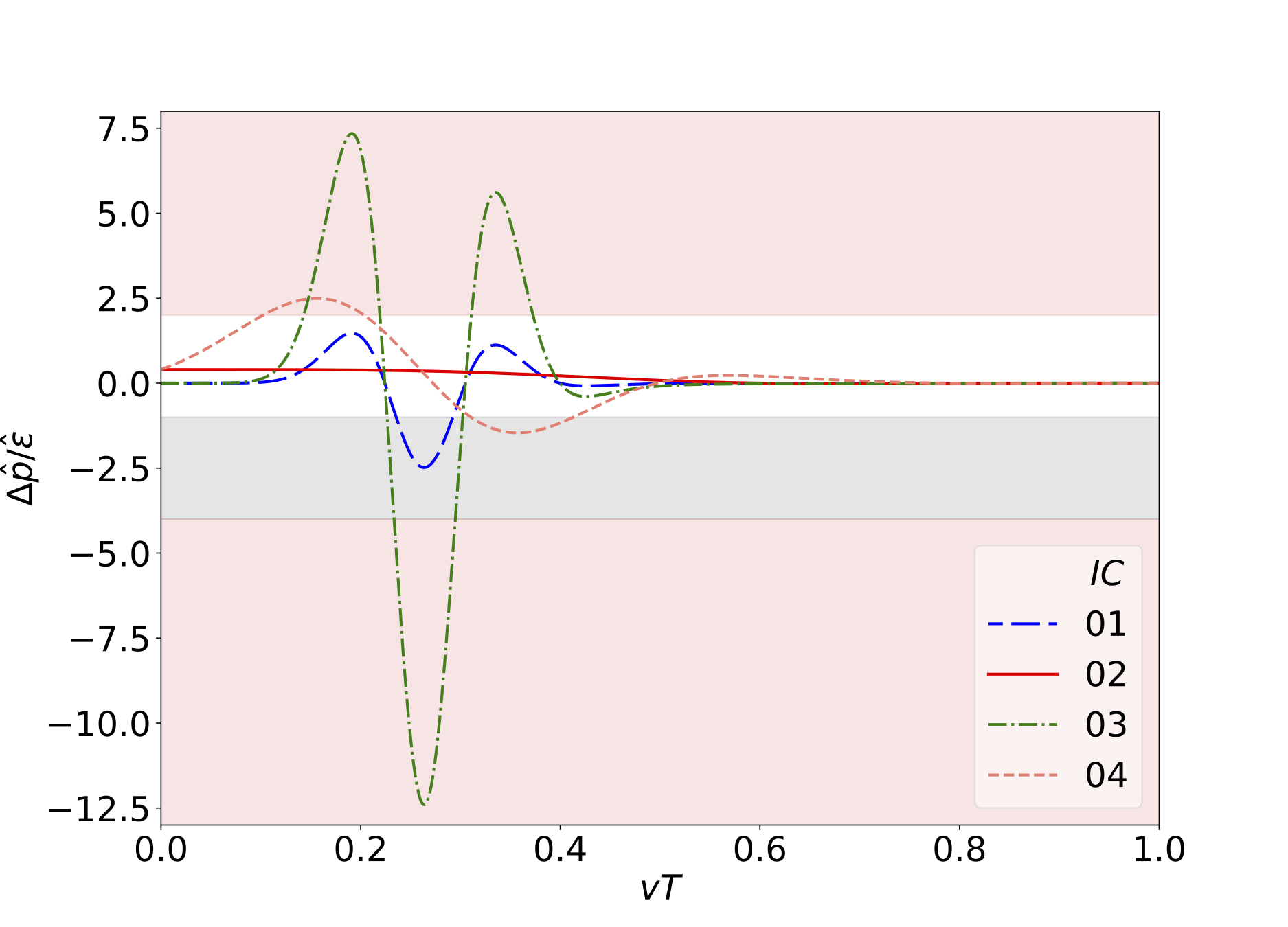
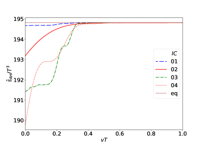
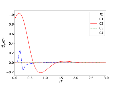
Figure 1: Numerical evolution of dimensionless ratios involving (a) the pressure anisotropy, (b) the non-equilibrium entropy density, and (c) the scalar condensate, all of them plotted for $\mu/T=0$. The initial conditions (ICs) are given in Table 1. In Fig. (a) for the pressure anisotropy, the salmon regions delimit the regions with WEC violation (which automatically imply DEC violation), while the gray region delimits the region with only DEC violation. In Fig. (b) the thin straight line gives the equilibrium value of the entropy density attained by the system at long times.

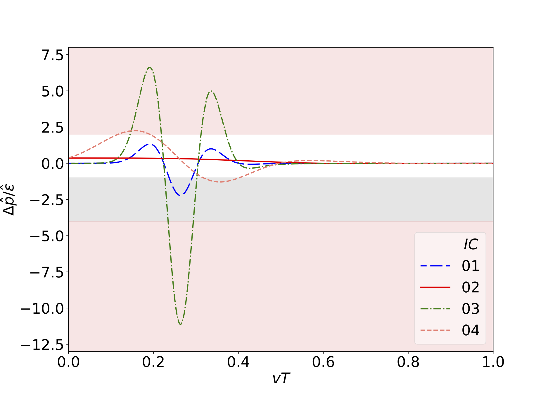
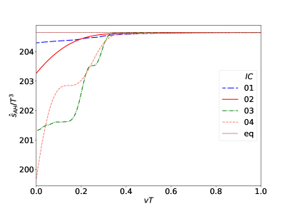
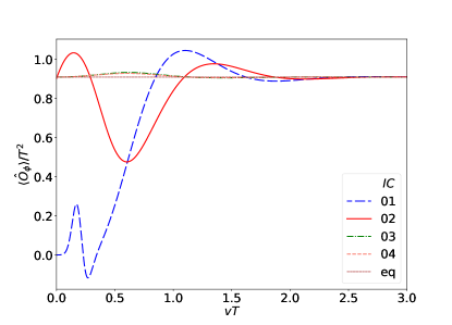
Figure 2: Numerical evolution of dimensionless ratios involving (a) the pressure anisotropy, (b) the non-equilibrium entropy density, and (c) the scalar condensate, all of them plotted for $\mu/T=1$. The initial conditions (ICs) are given in Table 1. In Fig. (a) for the pressure anisotropy, the salmon regions delimit the regions with WEC violation (which automatically imply DEC violation), while the gray region delimits the region with only DEC violation. In Figs. (b) and (c) the thin dashed lines give, respectively, the equilibrium value of the entropy density and of the scalar condensate attained by the system at long times.

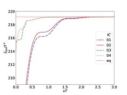
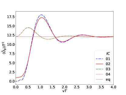
Figure 3: Numerical evolution of dimensionless ratios involving (a) the pressure anisotropy, (b) the non-equilibrium entropy density, and (c) the scalar condensate, all of them plotted for $\mu/T=\pi/\sqrt{2}$ (critical point). The initial conditions (ICs) are given in Table 1. In Fig. (a) for the pressure anisotropy, the salmon regions delimit the regions with WEC violation (which automatically imply DEC violation), while the gray region delimits the region with only DEC violation. In Figs. (b) and (c) the thin dashed lines give, respectively, the equilibrium value of the entropy density and of the scalar condensate attained by the system at long times.

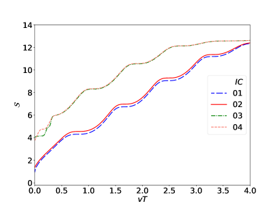
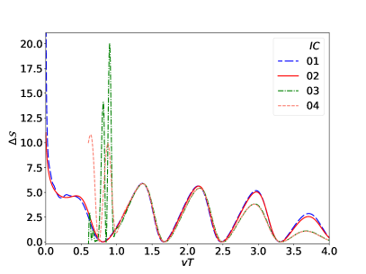
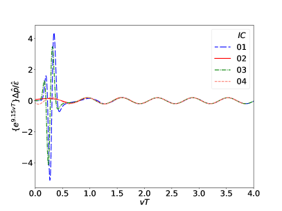
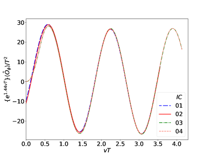
Figure 4: Time evolution of: (a) the logarithmic function $\mathcal{S}$ defined in Eq. (39); (b) its first finite difference $\Delta\mathcal{S}$ (with the curves shifted to visually overlap); (c) the harmonic part of the pressure anisotropy (also with the curves shifted to visually overlap); (d) the harmonic part of the scalar condensate (also with the curves shifted to visually overlap). The initial conditions (ICs) are given in Table 1 and are plotted here for $\mu/T=\pi/\sqrt{2}$ (critical point).

In Figs. 1, 2, and 3 we display the numerical time evolution for the different physical observables considering the initial data discussed in the previous section. One can notice that typically the scalar condensate only approaches its asymptotic equilibrium value for each $\mu/T$ at considerably larger times than the pressure anisotropy and the entropy density. Furthermore, for some initial data preserving all the energy conditions discussed before, one can observe transient violations of the DEC and even of the WEC when the fluid is still far from thermodynamic equilibrium. This has been also observed before for the 1RCBH model undergoing Bjorken flow [9] (and, as a particular case, also in the Bjorken flow of the SYM plasma [7, 8]), however, differently than in Bjorken flow, for the homogeneous isotropization dynamics of the 1RCBH model such energy condition violations are generally reduced as one increases the value of $\mu/T$.

Also as in the Bjorken flow, we observe for some initial data the formation of transient plateaus with zero entropy production when the system is still far from thermodynamic equilibrium. However, the interplay of these far from equilibrium plateaus and transient violations of energy conditions measured by the behavior of the pressure anisotropy is more complicated in the homogeneous isotropization dynamics. In fact, not all far from equilibrium plateaus in the entropy density are anticipating a posterior violation of energy conditions in the pressure anisotropy in the case of the homogeneous isotropization dynamics.

Moreover, from the analysis of several time evolutions of different initial conditions, for which figures 1 – 3 are quite representative, we observed for any considered value of $\mu/T$ the formation of multiple plateaus in the form of a stairway close to the respective equilibrium value for the entropy density. This fact could easily have gone unnoticed due to the very close proximity of such plateaus (which requires a high numerical precision to be resolved). To clearly display this peculiar behavior we constructed the following logarithmic function with the non-equilibrium entropy density $\hat{s}_{\textrm{AH}}(vT;\mu/T)$ and its asymptotic equilibrium value $\hat{s}_{\textrm{eq}}(\mu/T)$,

$$\mathcal{S}(vT;\mu/T)=\ln\left\{\frac{\hat{s}_{\textrm{eq}}(\mu/T)}{\hat{s}_{\textrm{eq}}(\mu/T)-\hat{s}_{\textrm{AH}}(vT;\mu/T)}\right\}.$$ (39)

This led us to realize that the stairway to equilibrium entropy comprises a periodic formation of ever increasing plateaus asymptotically approaching its ceil value. In order to determine such a period at the critical point of the model as displayed in Fig. 4, we calculated the finite difference of Eq. (39) to establish where the minima and maxima of $\mathcal{S}(vT;\mu/T)$ were. We then made use of the well known software harminv [79] to evaluate the mean value of the frequency of such extrema by means of the calculation of the second finite difference of Eq. (39), which gave us, at the critical point (CP),

$$\frac{\nu_{\cal{S}}^{CP}}{T}=(1.246\pm 0.004)\,\,\Rightarrow\,\,\tau_{\cal{S}}^{CP}T\approx(0.803\pm 0.003).$$ (40)

The periodicity of the oscillations of the pressure anisotropy near equilibrium is given by the real part of the lowest quasinormal frequency of the $SO(3)$ quintuplet channel of the 1RCBH model [10, 61]. On the other hand, the exponential decay of such oscillations is associated to the imaginary part of that complex quasinormal frequency. In Fig. 4 (c) we removed the aforementioned exponential damping and employed the harminv software to obtain the harmonic frequency of the pressure anisotropy oscillations near equilibrium evaluated at the critical point,

$$\frac{\mathrm{Re}\left[\nu_{p}^{CP}\right]}{T}=(1.54887\pm 0.00002)\,\,\Rightarrow\,\,\mathrm{Re}\left[\tau_{p}^{CP}\right]T\approx(0.645632\pm 0.000008).$$ (41)

The above result agrees with the real part of the lowest quasinormal frequency of the $SO(3)$ quintuplet channel of the 1RCBH model at the critical point as calculated in [10].

Furthermore, the periodicity of the oscillations of the scalar condensate near equilibrium is given by the real part of the lowest quasinormal frequency of the $SO(3)$ singlet channel of the 1RCBH model [10]. On the other hand, the exponential damping of such oscillations is associated to the imaginary part of that complex quasinormal frequency. In Fig. 4 (d) we removed the aforementioned exponential decay and used the harminv software to obtain the harmonic frequency of the scalar condensate oscillations near equilibrium evaluated at the critical point,

$$\frac{\mathrm{Re}\left[\nu_{\langle\hat{O}\rangle}^{CP}\right]}{T}=(0.60804\pm 0.00005)\,\,\Rightarrow\,\,\mathrm{Re}\left[\tau_{\langle\hat{O}\rangle}^{CP}\right]T\approx(1.6446\pm 0.0001).$$ (42)

The above result agrees with the real part of the lowest quasinormal frequency of the $SO(3)$ singlet channel of the 1RCBH model at the critical point as calculated in [10].

In Fig. 4 we show, for the four initial conditions in Table 1 evaluated at the critical point $\mu/T=\pi/\sqrt{2}$, the logarithmic function $\mathcal{S}$ defined in Eq. (39), its first finite difference $\Delta\mathcal{S}$ with each curve shifted to visually overlap for presentation purposes of our main results, and the harmonic parts of the pressure anisotropy and of the scalar condensate oscillations, also shifted to visually overlap. From the results in Eqs. (40), (41) and (42) one sees that at the critical point the period of plateau formation in the stairway to equilibrium entropy is $\sim 24\%$ larger than the period of harmonic oscillations of the pressure anisotropy close to thermodynamic equilibrium, while being $\sim 51\%$ smaller than the period of harmonic oscillations of the scalar condensate in the linear regime.

Finally, as aforementioned, the purely thermal SYM plasma is obtained as a particular case of the 1RCBH model by turning off the Maxwell and the dilaton fields in the bulk, implying zero chemical potential and vanishing scalar condensate for the dual quantum field theory at the boundary. For the SYM plasma we obtained that the period of plateau formation in the stairway to equilibrium entropy ($\tau_{\cal{S}}^{\textrm{SYM}}T\sim 0.32$) is half the period of harmonic oscillations of the pressure anisotropy in the linear regime ($\mathrm{Re}\left[\tau_{p}^{\textrm{SYM}}\right]T\sim 0.64$).

IV Conclusions

In the present work, we analyzed the homogeneous isotropization dynamics of the top-down 1RCBH holographic model, including for the first time the calculation of the time evolution of its non-equilibrium entropy density. We found that generally the scalar condensate takes a considerably longer time than the pressure anisotropy and the entropy density to approach the respective equilibrium values. Furthermore, for some initial data preserving all the energy conditions, transient violations of the dominant and even of the weak energy conditions are observed when the fluid is still far from thermodynamic equilibrium, with the magnitude of such violations getting reduced as the chemical potential of the medium is increased (contrary to what happens in the Bjorken flow of the same model).

Moreover, a new feature disclosed in the present work is the formation of a stairway to equilibrium entropy at late times. This stairway is observed for all the initial data analyzed undergoing homogeneous isotropization dynamics in the 1RCBH model and comprises the formation of a periodic sequence of several close plateaus in the entropy density near thermodynamic equilibrium. We calculated the period of formation of such near-equilibrium plateaus for the entropy density and found that, at the critical point, it is $\sim 24\%$ larger than the period of harmonic oscillations of the pressure anisotropy around zero, and $\sim 51\%$ smaller than the period of harmonic oscillations of the scalar condensate around its equilibrium value. On the other hand, for the particular case of the purely thermal SYM plasma at zero chemical potential, the period of plateau formation in the stairway to equilibrium entropy is half the period of harmonic oscillations of the pressure anisotropy around zero when the system is near thermodynamic equilibrium.

As far as we know, such a stairway structure, which requires high numerical precision to be resolved due to the close proximity of the near-equilibrium plateaus for the entropy, is a peculiar feature that has never been reported before in the literature and deserves further investigation. In fact, it would be interesting to obtain the period of plateau formation in the stairway to equilibrium entropy for all the possible values of the dimensionless ratio $\mu/T\in[0,\pi/\sqrt{2}]$, while here we only calculated it for the two extrema of this interval, corresponding respectively to the neutral SYM plasma and to the case of the critical point of the 1RCBH model. This is a time demanding task which we postpone for a future work. Moreover, the physical mechanism behind the stairway to equilibrium entropy in the present model is currently unknown. In these regards, possibly the implementation of machine learning techniques can help in the task of recognizing non-obvious patterns and correlations between different observables, as in the recent work of Ref. [80]. In this last work, a deep neural network applied to a different holographic model allowed for the reconstruction of the boundary non-equilibrium entropy from data concerning some characteristic features of the boundary pressure anisotropy. We hope to report progress in this direction in the near future.