From zero-mode intermittency to hidden symmetry in random scalar advection

Abstract

The statistical behavior of scalars passively advected by random flows exhibits intermittency in the form of anomalous multiscaling, in many ways similar to the patterns commonly observed in incompressible high-Reynolds fluids. This similarity suggests a generic dynamical mechanism underlying intermittency, though its specific nature remains unclear. Scalar turbulence is framed in a linear setting that points towards a zero-mode scenario connecting anomalous scaling to the presence of statistical conservation laws; the duality is fully substantiated within Kraichnan theory of random flows. However, extending the zero-mode scenario to nonlinear settings faces formidable technical challenges. Here, we revisit the scalar problem in the light of a hidden symmetry scenario introduced in recent deterministic turbulence studies addressing the Sabra shell model and the Navier-Stokes equations. Hidden symmetry uses a rescaling strategy based entirely on symmetry considerations, transforming the original dynamics into a rescaled (hidden) system; It ultimately identifies the scaling exponents as the eigenvalues of a Perron-Frobenius operator acting on invariant measures of the rescaled equations. Considering a minimal shell model of scalar advection of the Kraichnan type that was previously studied by Biferale & Wirth, the present work extends the hidden symmetry approach to a stochastic setting, in order to explicitly contrast it with the zero-mode scenario. Our study indicates that the zero-mode scenario represents only one facet of intermittency, here prescribing the scaling exponents of even-order correlators. Besides, we argue that hidden symmetry provides a more generic mechanism, fully prescribing intermittency in terms of scaling anomalies, but also in terms of its multiplicative random nature and fusion rules required to explicitly compute zero-modes from first principles.

I Introduction

A hallmark feature of turbulent environments is their apparent lack of statistical self-similarity, a feature commonly referred to as spatial intermittency. While such phenomenology is successfully captured by statistical frameworks involving multifractal random processes of various complexities [1, 2, 3, 4, 5, 6], the dynamical origin of multiscaling from the original equations is not fully clear. On the one hand, it has long been suggested that the presence of multifractal scaling reflects the spontaneous breaking of spatio-temporal symmetry of the Navier-Stokes (NS) equations and related models, which is not restored in the vanishing viscosity limit even at a statistical level [7, 8]. This qualitative viewpoint has been recently substantiated by a series of work pointing towards the presence of a weaker (hidden) symmetry, which appears under a suitable dynamical rescaling of the space-time variables [9, 10, 11, 12]. The hidden symmetry implies a form of scale-invariance weaker than monofractal scaling, which appears for example when considering ratios of increments such as Kolmogorov multipliers [7, 13, 14, 15, 16]. In simplified models at least, the hidden symmetry was shown to provide a generic mechanism for spatial intermittency [17, 10, 18], in the sense that it fully determines the anomalous exponents of the structures functions in terms of the eigenvalues of a Perron-Frobenius operator acting on invariant measures of the rescaled equations.

On the other hand, a different route to intermittency is the zero-mode mechanism, which emerges in a simpler linear turbulence problem. Namely, consider the advective-diffusive transport equation

$$\partial_{t}\theta+{\bf u}\cdot\nabla\theta=\kappa\Delta\theta+{\bf f}$$ (1)

for a passive substance $\theta({\bf x},t)$, where ${\bf u}({\bf x},t)$ is a prescribed carrier flow, ${\bf f}({\bf x},t)$ is a stirring force and $\kappa$ is a diffusion coefficient. One naturally has in mind cases when the carrier flow solves the NS, a situation for which the passive scalar is known to develop spatial intermittency in the form of ramp-cliffs structures [19, 20]. An instructive and solvable framework however emerges when one uses as a proxy for fully developed turbulence a (non-intermittent) Markovian monofractal Gaussian field: This is the framework of the Kraichnan flow theory, which by cutting through much of the difficulties of turbulence theory provides a rigorous connection between statistical conservation laws of fluid particles and anomalous scaling of the transported field [21, 22, 23, 24, 25, 26, 27, 28].

The purpose of the present paper is to revisit the scalar problem, in order to highlight a connection between the two distinct mechanisms for intermittency: zero-mode and hidden symmetry. In Eq. (1), a technical difficulty comes from the fact that scalar transport involves a stochastic partial differential equation. While Kraichnan flow theory gives a meaning to Eq. (1) for a Markovian carrier flow, we here prefer to bypass this issue by considering the shell-model version of Eq. (1), where the multiscale nature of the scalar dynamics is represented by a (discrete) sequence $\theta_{n}$ associated to a geometric sequence of scales $\ell_{n}\propto\lambda^{-n}$, and which is known to exhibit spatial intermittency in the form of anomalous scaling laws for the scalar structure functions [29, 30, 31, 32, 33, 34]. On the one hand, our work highlights the fact that the presence of zero-mode solutions stem from two specific ingredients: statistical conservation laws and algebraic decay of correlation functions for non-diagonal terms, a heuristic feature known as fusion rules. On the other hand, we argue that the hidden symmetry is a more general mechanism, which not only prescribes the anomalous scaling but also prescribes the fusion rules and the multifractal formalism.

The paper is organized as follows. §II presents the shell model and its general phenomenology. §III describes the zero-mode mechanism to intermittency and its connection to statistical conservation laws. For the sake of exposition, we here only focus on second and fourth-order structure functions, since the situation with higher order is similar but technically more sophisticated [32]. §IV discusses scaling symmetries and introduces the hidden scaling symmetry as a non-linear scale invariance for a suitably defined non-linear rescaled system. §V describes the Perron-Frobenius scenario to anomalous scaling laws, which we derive from the hypothesis of statistical restoring of hidden scaling symmetry. §VI highlights the implications of the Perron-Frobenius for the zero-mode scenario, and its connections with the multifractal formalism. §VII sketches some concluding remarks. In order to facilitate navigation throughout the manuscript, some technicalities are pushed to the Appendices A–D.

II Shell model for random advection

The rationale beneath random shell models for a passive scalar [30, 31, 32] follows the usual interpretation of shell models of turbulence [8, 35], in which a multiscale dynamics is represented with a geometric sequence of scales $\ell_{n}=\ell_{0}\lambda^{-n}$. Here, $n\in\mathbb{Z}$ is an integer shell number and $\lambda>1$ is a fixed intershell ratio usually taken equal to $2$ or fractional powers of $2$. Corresponding wavenumbers are introduced as $k_{n}=1/\ell_{n}=k_{0}\lambda^{n}$. At each scale, increments of a velocity field are modeled with a shell velocity $u_{n}(t)\in\mathbb{R}$ and increments of a scalar field by a shell scalar $\theta_{n}(t)\in\mathbb{R}$; both are real variables depending on time $t$. A minimal shell model accounting for passive scalar transport can be formulated as [29, 31, 34]

$$\left(\frac{d}{dt}+\kappa k_{n}^{2}\right)\theta_{n}=k_{n}\theta_{n+1}u_{n}-k_{n-1}\theta_{n-1}u_{n-1},$$ (2)

with $\kappa k_{n}^{2}$ representing diffusion term, involving the diffusion coefficient $\kappa\geq 0$. The right-hand side of Eq. (2) is a bilinear advection term restricted to nearest neighbors. It is designed such that the unforced ideal system (with $\kappa=0$) conserves the scalar energy $E_{\theta}=\sum\theta_{n}^{2}$; see §II.2 below.

We consider constant boundary conditions at shells $n\leq 0$ and $n>n_{\max}$ as

$$\theta_{n}(t)\equiv\left\{\begin{array}[]{ll}1,&n\leq 0;\\[2.0pt] 0,&n>n_{\max}.\end{array}\right.$$ (3)

The unit value at shell $n=0$ plays the role of constant large-scale forcing. The shell-number cutoff $n_{\max}$ plays the role of a Galerkin truncation, which is convenient to avoid technical difficulties and necessary for numerics. Because interactions are restricted to neighboring shells, setting the shells $n<0$ to a constant (e.g., unit) value is a conventional choice that does not affect the dynamics, but later proves convenient for the exposition of hidden symmetry. Let us also point out that the theory is essentially limited only by the form of symmetries and conservation laws; see [10]. Hence, the restriction to real shell variables as well as to the so-called dyadic or Desnyansky-Novikov nonlinearity in the shell model (2) is chosen for the simplicity of representation, but is not a limitation of our theory.

II.1 Random scalar advection

The idea of Kraichnan [21, 26, 27, 28] is to consider the advection Eq. (1) with random Gaussian velocity fields, white in time and scale-invariant in space. Similarly, in the shell model (2), we consider random, Gaussian shell velocities $u_{n}(t)$ with the correlation functions

$$\left\langle u_{n}(t)u_{n^{\prime}}(t^{\prime})\right\rangle=U_{0}^{2}\tau_{0}\,\lambda^{-n\xi}\delta(t-t^{\prime})\delta_{nn^{\prime}}.$$ (4)

The factor $\lambda^{-n\xi}$ mimics a rough (Hölder continuous) scale-invariant velocity field with the roughness parameter $0<\xi<2$. The transport rate is controlled by the typical velocity $U_{0}$ and associated timescale $\tau_{0}=\ell_{0}/U_{0}$. Now, in order to transform Eq. (2) into a SDE, one replaces the advecting velocities in Eq. (2) as

$$u_{n}(t)\,dt\ \mapsto\ U_{0}\tau_{0}^{1/2}\,\lambda^{-n\xi/2}dw_{n}(t),$$ (5)

where $w_{n}(t)$, $n\in\mathbb{Z}$, are independent real Wiener processes. Expressing also $k_{n}=k_{0}\lambda^{n}$, elementary manipulations reduce Eq. (2) to the form [30]

$$\begin{split}&d\theta_{n}=\tau_{0}^{-1/2}\left(\gamma^{n}\theta_{n+1}\circ dw_{n}-\gamma^{n-1}\theta_{n-1}\circ dw_{n-1}\right)-\kappa k_{n}^{2}\theta_{n}\,dt,\end{split}$$ (6)

involving $\gamma=\lambda^{1-\xi/2}$ as the relevant velocity scaling parameter from the interval $1<\gamma<\lambda$. With the rescaling $w_{n}\to w_{n}/\tau_{0}^{1/2}$, $t\to t/\tau_{0}$, Eq. (6) takes the dimensionless form

$$d\theta_{n}=\gamma^{n}\theta_{n+1}\circ dw_{n}-\gamma^{n-1}\theta_{n-1}\circ dw_{n-1}-\mathrm{Pe}^{-1}\,\lambda^{2n}\theta_{n}\,dt,$$ (7)

where $\mathrm{Pe}=U_{0}\ell_{0}/\kappa$ is the dimensionless Péclet number.

Equation (7) is written using the Stratonovich convention and ensures the scalar energy conservation [36]; see Section II.2 below. For further derivations, we prefer using the Itô stochastic calculus. Let us use the short notation $\theta=\big{(}\theta_{n}\big{)}_{n\in\mathbb{Z}}$ and $dw=\big{(}dw_{n}\big{)}_{n\in\mathbb{Z}}$ for bi-infinite sequences. Using the Stratonovich to Itô conversion formula [37] and boundary conditions (3), one obtains the Itô SDE version of Eq. (7) as

$$d\theta_{n}=\mathcal{N}_{n}[\theta,dw]+(I_{n}+B_{n}-D_{n})\theta_{n}\,dt,\quad 1\leq n\leq n_{\max},$$ (8)

where we denoted the advection terms by

$$\mathcal{N}_{n}[\theta,dw]=\gamma^{n}\theta_{n+1}dw_{n}-\gamma^{n-1}\theta_{n-1}dw_{n-1}.$$ (9)

The drift terms combine Itô drifts, boundary and diffusion terms, respectively:

$$\begin{split}I_{n}=-\frac{\gamma^{2n}+\gamma^{2n-2}}{2},\quad B_{n}=\dfrac{\delta_{n1}}{2}+\dfrac{\delta_{nn_{\max}}\gamma^{2n}}{2},\quad D_{n}=\mathrm{Pe}^{-1}\lambda^{2n},\end{split}$$ (10)

where $\delta_{n1}$ and $\delta_{nn_{\max}}$ are the Kronecker deltas. The coefficients $B_{n}$ retain the boundary effects at $n=1$ and $n_{\max}$. We refer to Eqs. (8)–(10) with the boundary conditions (3) as the Kraichnan-Wirth-Biferale (KWB) shell model for random advection, following its explicit description as a minimal scalar model in [34].

II.2 Balance of scalar energy and the inertial interval

We define the scalar energy at shell $n$ as $\theta_{n}^{2}$, and denote its average over random realizations of the velocity ensemble as $\left\langle\theta_{n}^{2}\right\rangle$. Using Itô’s lemma [37] with Eqs. (8)–(10) and (3), one derives the balance for averaged scalar energy at every shell $1\leq n\leq n_{\max}$ as (see [30, 34] and Appendix A)

$$\dfrac{d\left\langle\theta_{n}^{2}\right\rangle}{dt}=\Pi_{n-1}-\Pi_{n}-2D_{n}\left\langle\theta_{n}^{2}\right\rangle.$$ (11)

Here $\Pi_{n}$ represents the energy flux from shell $n$ to $n+1$ due to advection, which is expressed as

$$\Pi_{n}=\left\{\begin{array}[]{ll}1,&n=0;\\[2.0pt] \gamma^{2n}\left\langle\theta_{n}^{2}\right\rangle-\gamma^{2n}\left\langle\theta_{n+1}^{2}\right\rangle,&n=1,\ldots,n_{\max}-1;\\[2.0pt] 0&n=n_{\max}.\end{array}\right.$$ (12)

We are interested in the regime of developed turbulence corresponding to very large Péclet numbers. The phenomenological description of scalar dynamics then follows the usual interpretation of a turbulent cascade: The scalar energy injected with rate $\Pi_{0}=1$ from the forcing range $k_{n}/k_{0}\sim 1$ is transferred to small diffusive scales

$$\frac{k_{n}}{k_{0}}=\lambda^{n}\sim\mathrm{Pe}^{1/\xi},$$ (13)

where it is absorbed [8, 30]. The condition (13) is obtained by comparing the diffusion term in Eq. (11) with the flux term (12), which yields $\gamma^{2n}\sim D_{n}=\mathrm{Pe}^{-1}\lambda^{2n}$ with $\gamma=\lambda^{1-\xi/2}$.

The present work will focus on describing the statistical properties within the (inertial) interval of scales at which both the forcing and diffusion terms are negligible. The inertial interval corresponds to the wavenumbers satisfying the conditions

$$1\ll\frac{k_{n}}{k_{0}}\ll\mathrm{Pe}^{1/\xi}.$$ (14)

In terms of shell numbers, it reads $0\ll n\ll n_{K}$ with the diffusive (Kolmogorov) shell number

$$n_{K}=\dfrac{1}{\xi}\log_{\lambda}\mathrm{Pe}.$$ (15)

Neglecting the forcing and diffusion terms in Eq. (8) yields

$$d\theta_{n}=\mathcal{N}_{n}[\theta,dw]+I_{n}\theta_{n}\,dt,\quad n\in\mathbb{Z},$$ (16)

to which we refer as the ideal KWB model. We remark that neglecting the large-scale (forcing) and small-scale (diffusion) cutoffs implies that the ideal KWB model is considered formally for arbitrary $n\in\mathbb{Z}$. The energy balance provided by Eqs. (11) and (12) reduces in the inertial interval to

$$\dfrac{d\left\langle\theta_{n}^{2}\right\rangle}{dt}=\Pi_{n-1}-\Pi_{n}=\gamma^{2n-2}\left\langle\theta_{n-1}^{2}\right\rangle-(\gamma^{2n-2}+\gamma^{2n})\left\langle\theta_{n}^{2}\right\rangle+\gamma^{2n}\left\langle\theta_{n+1}^{2}\right\rangle.$$ (17)

Please observe that, from mathematical point of view, the study of inertial interval statistics is formulated as the asymptotic analysis of the KWB model (8) in the limit

$$t\to\infty,\quad n_{\max}\to\infty,\quad\mathrm{Pe}\to\infty,\quad n\to\infty,$$ (18)

where the limits are considered successively from left to right. These limits signify the large-time asymptotic (or time averaging), removal of small-scale cutoff, vanishing diffusion limit and, finally, small-scale asymptotic.

II.3 Numerical model

Theoretical assumptions and conclusions of this paper are verified with numerical simulations designed to give accurate statistics in a large inertial interval. Our numerical model is given by Eqs. (8)–(10) with the boundary conditions (3), where we set $\lambda=2^{1/3}$, $n_{\max}=36$ and $\mathrm{Pe}=\lambda^{n_{K}\xi}\approx 140$ with $n_{K}=32$ and $\xi=2/3$. We expect that the inertial interval statistics does not depend on a specific form of the diffusion mechanism, except perhaps from finite-$\mathrm{Pe}$ effects [30, 31]. For our numerical analysis, it proves convenient to set $D_{n}=0$ for the shells $n<n_{K}$, i.e., removing the diffusion term completely from Eq. (8) in the inertial interval. With this choice, the energy balance (17) is exactly satisfied for at shells $n=1,\ldots,n_{K}-1$.

Our numerical simulations of the KWB dynamics rely on Milstein scheme [38], which is here relatively simple to implement because the advection terms $\mathcal{N}_{n}[\theta,dw]$ are linear with respect to $\theta$. This scheme yields the increment at one time step $\Delta t$ as

$$\Delta\theta_{n}=\mathcal{N}_{n}(\theta,\Delta W)+(I_{n}+B_{n}-D_{n})\theta_{n}\Delta t+\,\dfrac{1}{2}\gamma^{2n}\theta_{n}\left(\Delta t-\Delta W_{n}^{2}\right)+\gamma^{2n-2}\theta_{n}\left(\Delta t-\Delta W_{n-1}^{2}\right),$$ (19)

where the $\Delta W_{n}$’s are independent random numbers drawn from a centered Gaussian distribution $\sqrt{\Delta t}\;\mathcal{N}(0,1)$ with variance $\Delta t$. We use the integration step $\Delta t=5\times 10^{-7}$ and generate an ensemble of realizations in a steady state using a Monte-Carlo sampling as follows. Initially, we perform a run until time $T=10^{3}$ and then select the last time to seed $100$ different simulations, which differ from each other by the realization of the noise. Each simulation is integrated until $T=10^{3}$ with data output every time interval of $5\times 10^{-3}$, resulting in $2\times 10^{5}$ outputs per realization. Averages and densities are therefore computed using $2\times 10^{8}$ points per shell number. Examples of times series and distributions are shown in Figure 1(a).

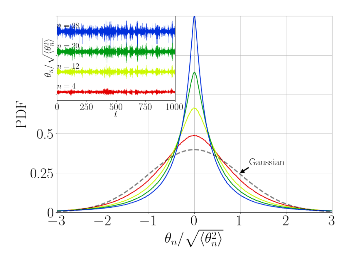
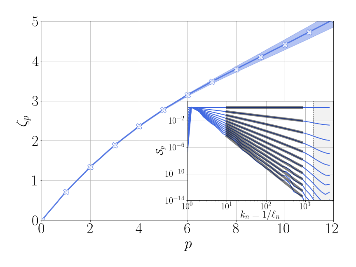
Figure 1: (a) PDF of inertial-range shell variables normalised by their variance. Inset shows corresponding time-serie realizations. (b) Scaling exponents $\zeta_{p}$. Inset shows power law scalings of structure functions for the integer orders from $p=0$ (top) to $p=10$ (bottom), with the grey thick lines indicating the scaling region.

III Zero-mode scenario to anomalous scaling laws

Structure functions are traditional observables for the analysis of intermittency in fully developed turbulence [8]. In shell models, they are usually defined as the time-ensemble averaged moments

$${\mathcal{S}}_{p}(\ell_{n})=\lim_{T\to\infty}T^{-1}\int_{0}^{T}\langle|\theta_{n}|^{p}\rangle\,dt.$$ (20)

In the inertial range, the KWB model is known to exhibit power-law scaling laws ${\mathcal{S}}_{p}(\ell_{n})\propto\ell_{n}^{\zeta_{p}}$ with non-linear (anomalous) behavior of the exponents $\zeta_{p}$. This distinctive feature reflects the lack of statistical scale-invariance for the distributions of the shell variables [8] – See Figure 1. For even-order structure functions, the presence of anomalous exponents can be explicitly related to a zero-mode mechanism. Following [31, 32], the present section briefly accounts for the zero-mode theory at the level of second and fourth-order correlators. We also point out that the presence of zero-modes reflects the presence of exact statistical conservations laws in the ideal model.

III.1 Second-order structure functions

Performing the time-average of the energy balance in the inertial interval, namely Eq. (17), the left-hand side vanishes. This implies in particular that the mean flux of scalar energy is constant in the inertial interval, prescribed by injection condition $\Pi_{0}=1$, consistent with the phenomenology of §II.2. Besides, replacing $\left\langle\theta_{n}^{2}\right\rangle$ by their time averages from Eq. (20), and cancelling the common factor $\gamma^{2n-2}$ in Eq. (17) yields the recursion

$${\mathcal{S}}_{2}(\ell_{n-1})-(1+\gamma^{2})\mathcal{S}_{2}(\ell_{n})+\gamma^{2}S_{2}(\ell_{n+1})=0.$$ (21)

System (21) is linear and has two independent solutions given (up to a constant factor) by $\mathcal{S}_{2}(\ell_{n})\propto\gamma^{-2n}=\lambda^{-(2-\xi)n}$ and $\mathcal{S}_{2}(\ell_{n})\propto 1$. We rule out the second solution, because it does not decrease at small scales. Hence, one derives the scaling law [30]

$$\mathcal{S}_{2}(\ell_{n})\propto\ell_{n}^{\zeta_{2}}\ \ \text{with}\ \ \zeta_{2}=2-\xi.$$ (22)

The exponent $\zeta_{2}$ provides a non-vanishing energy flux (12) from large to small scales through the inertial interval. This property is analogous to the relation of the third-order structure function with the energy flux in turbulence [8]. In our numerics, the scaling (22) is indeed observed over almost three decades – see Fig. 2(a).

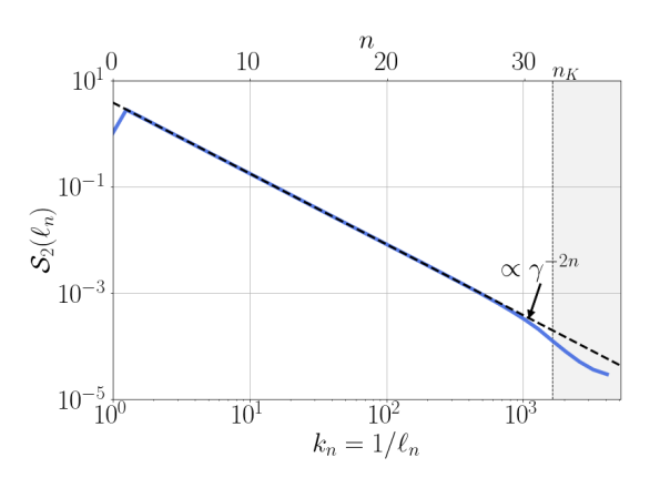
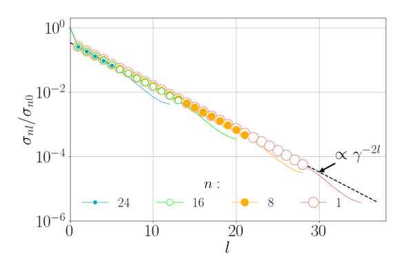
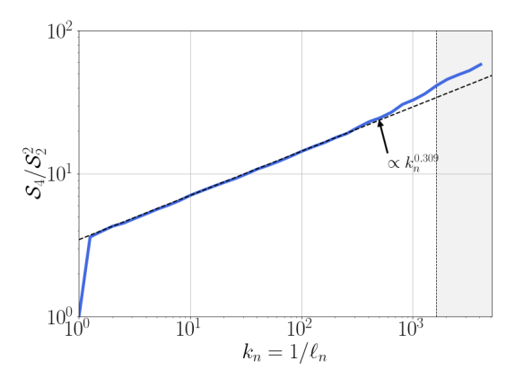
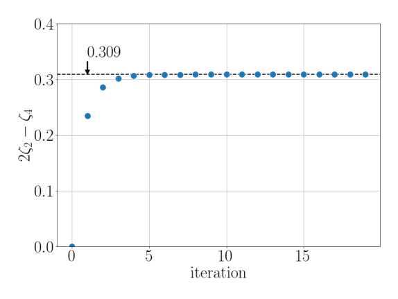
Figure 2: (a) Second order structure function with the Kolmogorov scaling $S_{2}(\ell_{n})=\ell_{n}^{\zeta_{2}}$. (b) Collapse of off-diagonal terms $\sigma_{nl}/\sigma_{n0}$. Dots indicate the inertial interval $1\leq n,n+l\leq 28$. (c) Flatness with the zero-mode scaling exponent $2\zeta_{2}-\zeta_{4}\simeq 0.309$. (d) Convergence of the iteration procedure to the zero-mode scaling exponent.

Please observe, that the scaling solution (22) is an example, simple but not trivial, of a zero-mode. Recasting the recursion (21) in matrix form, it is expressed as the three-diagonal linear problem

$$\begin{pmatrix}{\ddots}\ \ \ &\ddots&\\ \ddots\ \ \ &-(1+\gamma^{2})&\ \gamma^{2}\ &\\ &\ 1\ &-(1+\gamma^{2})&\ \ \ \ddots\\ &&\ddots&\ddots\\ \end{pmatrix}\begin{pmatrix}\vdots\\ \mathcal{S}_{2}{(\ell_{n})}\\ \mathcal{S}_{2}{(\ell_{n+1})}\\ \vdots\end{pmatrix}=\begin{pmatrix}\vdots\\ 0\\ 0\\ \vdots\end{pmatrix},$$ (23)

solved with the conditions $\mathcal{S}_{2}(\ell_{n})\to 0$ as $n\to\infty$ (small-scale) and $\mathcal{S}_{2}(\ell_{0})=1$ (large scale).

III.2 Fourth-order structure functions

In the KWB model, the scaling exponents associated to higher-order even correlators (20) are determined by solving zero-mode problems similar to (23). This is the zero-mode mechanism for intermittency, which we now demonstrate for fourth-order structure functions.

Let us extend definition (20) by considering the fourth-order structure functions, involving two different shells $n$ and $n+l$, as

$$\sigma_{nl}=\lim_{T\to\infty}T^{-1}\int_{0}^{T}\left\langle\theta_{n}^{2}\theta_{n+l}^{2}\right\rangle dt.$$ (24)

Clearly, one has $S_{4}(\ell_{n})=\sigma_{n0}$. Obtaining recursion relations for $\sigma_{nl}$ follows a pattern similar to the second-order case. Considering shells $n$ and $n+l$ from the inertial interval, Itô’s lemma [37] with the ideal model (16) yield (see Appendix A)

$$\begin{split}\gamma^{-2n-l}\dfrac{d}{dt}\left\langle\theta^{2}_{n}\theta^{2}_{n+l}\right\rangle=-a_{l}\left\langle\theta_{n}^{2}\theta_{n+l}^{2}\right\rangle&+b_{l}\left\langle\theta_{n}^{2}\theta_{n+l+1}^{2}\right\rangle+b_{l}\gamma^{-2}\left\langle\theta_{n}^{2}\theta_{n+l-1}^{2}\right\rangle\\ &+b_{-l}\left\langle\theta_{n+1}^{2}\theta_{n+l}^{2}\right\rangle+b_{-l}\gamma^{-2}\left\langle\theta_{n-1}^{2}\theta_{n+l}^{2}\right\rangle,\end{split}$$ (25)

with the coefficients

$$a_{l}=\gamma^{l}+\gamma^{-l-2}+\gamma^{-l}+\gamma^{l-2}+4\gamma^{-l}\delta_{l1},\quad b_{l}=\gamma^{l}+2\delta_{l0}.$$ (26)

Averaging Eq. (25) with respect to time then yields

$$-a_{l}\sigma_{nl}+b_{l}\sigma_{n(l+1)}+b_{l}\gamma^{-2}\sigma_{n(l-1)}+b_{-l}\sigma_{(n+1)(l-1)}+b_{-l}\gamma^{-2}\sigma_{(n-1)(l+1)}=0.$$ (27)

Similarly to the second-order case, the recursion (27) can be recast as

$$\sum_{n^{\prime},l^{\prime}}{\mathcal{M}}_{nl,n^{\prime}l^{\prime}}\sigma_{n^{\prime}l^{\prime}}=0,$$ (28)

where nonzero components ${\mathcal{M}}_{nl,n^{\prime}l^{\prime}}$ are readily expressed from Eq. (27). System (28) is the zero-mode problem for the collection of structure functions $\sigma=\left(\sigma_{nl}\right)$ and the linear operator ${\mathcal{M}}=({\mathcal{M}}_{nl,n^{\prime}l^{\prime}})$.

To select relevant zero-modes, one needs to specify boundary conditions. This is less obvious then in the second-order case. Following [39, 31, 35], a proper zero-mode solution is defined by the combined use of (i) a power-law scaling ansatz for the original structure function

$$S_{4}(\ell_{n})=\sigma_{n0}\propto\ell_{n}^{\zeta_{4}}$$ (29)

with the unknown exponent $\zeta_{4}$, and (ii) the so-called fusion rule ansatz

$$\sigma_{nl}=C_{l}\sigma_{n0}$$ (30)

with the unknown coefficients $C_{l}$. Clearly, $C_{0}=1$ as a consistency condition. Under the scaling and the fusion-rule ansatz, a relevant zero-mode of (28) together with the exponent $\zeta_{4}$ are specified through the boundary condition

$$C_{l}\to 0\textrm{ \ as \ }l\to\infty,$$ (31)

which requires that moments $\sigma_{nl}$ decrease for large $l$.

The solution proceeds as follows. Using relations (29) and (30), one expresses every term in Eq. (27) as a multiple of $\sigma_{n0}$. For example,

$$\sigma_{(n+1)(l-1)}=C_{l-1}\sigma_{(n+1)0}=C_{l-1}\lambda^{-\zeta_{4}}\sigma_{n0}.$$ (32)

In this way, after cancelling $\sigma_{n0}$, one reduces Eq. (27) to the form

$$\left\{\begin{split}&-a_{0}+2b_{0}C_{1}(1+\gamma^{-2}\lambda^{\zeta_{4}})=0,\quad l=0,\\ &-a_{l}C_{l}+b_{l}C_{l+1}+b_{l}\gamma^{-2}C_{l-1}+b_{-l}C_{l-1}\lambda^{-\zeta_{4}}+b_{-l}\gamma^{-2}C_{l+1}\lambda^{\zeta_{4}}=0,\quad l\geq 1.\end{split}\right.$$ (33)

Notice that the derivation in the case $l=0$ used the symmetry property following from Eq. (24), e.g., $\sigma_{n(-1)}=\sigma_{(n-1)0}$.

For large $l\gg 1$, we substitute coefficients (26) and write Eq. (33) asymptotically as

$$-(\gamma^{l}+\gamma^{l-2})C_{l}+\gamma^{l}C_{l+1}+\gamma^{l-2}C_{l-1}\approx 0,\quad l\gg 1,$$ (34)

where we neglected small terms with $\gamma^{-l}$. The asymptotic linear system (34) has two independent solutions defined (up to a constant factor) by $C_{l}\propto\gamma^{-2l}$ and $C_{l}\propto 1$. The boundary condition (31) rules out the second solution. The first solution yields a unique sequence $(C_{l})_{l\geq 0}$ with $C_{0}=1$ solving the system (33) for $l\geq 1$. Note that this solution depends on the yet unknown exponent $\zeta_{4}$. We now express $\lambda^{\zeta_{4}}$ from Eq. (33) for $l=0$ with coefficients (26) as

$$\lambda^{\zeta_{4}}=\frac{1+\gamma^{2}}{3C_{1}}-\gamma^{2}.$$ (35)

This is a nonlinear equation for the exponent $\zeta_{4}$ because $C_{1}$ depends on $\zeta_{4}$.

Solution of Eq. (35) can be found numerically with the following iteration procedure [31]. One takes $\zeta_{4}=2\zeta_{2}$ as the initial guess and computes the corresponding solution $(C_{l})_{l\geq 0}$ as described above. Then, the new corrected value of $\zeta_{4}$ is found from Eq. (35). This process is iterated until the convergence is attained; see Fig. 2(d). In our numerics, taking $\xi=2/3$ we obtain $\zeta_{4}\simeq 2.357$. This exponent deviates from the monofractal prediction, i.e., $\zeta_{4}\neq 2\zeta_{2}$. The deviation $\zeta_{4}-2\zeta_{2}\simeq-0.309$ provides the scaling exponent for the flatness $S_{2}(\ell_{n})/S_{2}^{2}(\ell_{n})\propto\ell_{n}^{\zeta_{4}-2\zeta_{2}}$, which increases at small scales. As shown in Fig. 2(c), the anomalous scaling for the flatness agrees with the zero-mode prediction over almost the full three decades of our numerics, with the deviations seen at the ultraviolet end being caused by finite-size effects. Besides, our numerics support the fusion rule ansatz (30). Figure 2(b) shows that the coefficients $\sigma_{nl}/\sigma_{n0}$ become indeed independent of the index $n$ when both $n$ and $n+l$ lie in inertial range, and feature the Kolmogorov scaling $C_{l}\propto\gamma^{-2l}$.

III.3 Limitations of the zero-mode theory

The approach based on zero-modes has several limitations, which refer both to the results and the formulation. (i) The formulation relies on a scaling ansatz (29) and on a fusion-rule ansatz (30): these assumptions are essentially heuristic and require separate explanations. (ii) The zero-mode mechanism is tied to the linear structure of the advection equation. In the KWB model, each zero-mode is accompanied by a corresponding statistical conservation law, which carries zero flux [40, 26]. To understand the origin of such conservation laws, one observes that both second and fourth order correlators satisfy linear systems (17) and (25). Zero-modes are stationary solutions, belonging to the null-space of the linear operator on the right-hand side; see Eqs. (23) and (28). Conservation laws are defined by the null space of the adjoint linear operators. We refer the reader interested in the details of the corresponding derivation to Appendix D. In nonlinear settings, numerical evidence for statistical conservation laws exists, that suggest relevance of the zero-mode mechanism, but a proper systematic formulation faces technical difficulties [41, 40]. (iii) The results are limited to even-order structure functions. Beyond the second and fourth order exponents considered above, the extension to arbitrary even orders is possible [32], but the power law scaling of structure functions for odd (or arbitrary real) orders $p$ cannot be justified in a similar way.

IV Classical vs Hidden scaling symmetries

We now present a different and more general approach on multiscaling based on the concept of hidden scaling symmetry. This symmetry emerges under a proper rescaling of the ideal model (16). This rescaling can be seen as a projection in phase space, which maps original variables to their ratios. We argue and verify numerically that the hidden symmetry is restored in the statistical sense at scales of the inertial interval, even though the original scaling symmetries get broken.

IV.1 Classical scaling symmetries

Let us first recall that the ideal model (16) possesses a family of scaling symmetries generated by the transformations

$$\theta_{n}\mapsto\lambda^{h}\theta_{n\pm 1},\quad w_{n}\mapsto\gamma^{\pm 1}w_{n\pm 1},\quad t\mapsto\gamma^{\pm 2}t.$$ (36)

The change of shell index $n\mapsto n+1$ (and similarly $n\mapsto n-1$) defines the spatial scaling by the factor of $\lambda$, since $\ell_{n+1}=\ell_{n}/\lambda$, while the exponent $h\in\mathbb{R}$ defines rescaling of scalar variables by an arbitrary factor $\lambda^{h}$. The change of time $t^{\prime}=\gamma^{2}t$ combined with the scaling $w^{\prime}_{n}=\gamma w_{n+1}$ yield $w^{\prime}_{n}(t^{\prime})=\gamma w_{n+1}(t^{\prime}/\gamma^{2})$, which is again a Wiener process [42]. While the (full) KWB dynamics (8)-(10) breaks the symmetries (36) at large and small scales due to the boundary conditions and diffusion, classical turbulence theory [8] postulates that these symmetries may be recovered in a statistical sense in the inertial interval, i.e., in the limits prescribed by Eq. (18). Because the family of symmetries (36) contains an arbitrary exponent $h$, one expects that the stationary measure exhibits a statistical intermittency in the form of multifractal scaling [1]. Heuristically, this means that the exponent $h$ is not selected univocally but rather as a probability distribution. The idea of hidden symmetry is that this degeneracy can be removed by a suitable rescaling (projection) of the phase space and time. The present section describes the construction for the KWB model.

IV.2 Shell-time rescaling

Given a sequence of scalars $\theta=(\theta_{n})_{n\in\mathbb{Z}}$, we introduce a sequence of scalar amplitudes $\mathcal{A}[\theta]=(\mathcal{A}_{n}[\theta])_{n\in\mathbb{Z}}$ as

$$\mathcal{A}_{n}[\theta]=\sqrt{\theta_{n}^{2}+\alpha\theta_{n-1}^{2}+\alpha^{2}\theta_{n-2}^{2}+\cdots},$$ (37)

where $\alpha$ is a fixed positive pre-factor. The amplitudes $\mathcal{A}_{n}[\theta]$ are positive and represent local averages of the scalar $\theta$ about the scale $\ell_{n}$. Later in §VI.3 we justify that the locality is ensured under the condition $\alpha<\lambda^{-2h_{\max}}$ with $h_{\max}\approx 1.4$.

Let us now fix a reference shell $m\geq 0$ and define the respective rescaled variables. Using the scalar amplitudes (37), we define the rescaled scalar $\Theta^{(m)}=\big{(}\Theta^{(m)}_{N}\big{)}_{N\in\mathbb{Z}}$, the rescaled Wiener process $W^{(m)}=\big{(}W_{N}^{(m)}\big{)}_{N\in\mathbb{Z}}$ and proper time $\tau^{(m)}$ as

$$\Theta_{N}^{(m)}=\frac{\theta_{m+N}}{\mathcal{A}_{m}[\theta]},\quad W_{N}^{(m)}=\gamma^{m}w_{m+N},\quad\tau^{(m)}=\gamma^{2m}t.$$ (38)

We note that $\big{(}W_{N}^{(m)}\big{)}_{N\in\mathbb{Z}}$ is still a sequence of independent Wiener processes in terms of the rescaled time $\tau^{(m)}$. For $m=0$, the boundary conditions (3) yield $\mathcal{A}_{0}[\theta]=1/\sqrt{1-\alpha}$, and Eq. (38) prescribes a linear rescaling. For $m>0$, the transformation (38) is nonlinear. Using Eqs. (37) and (38), one can verify the identity, valid for all $m\geq 0$:

$$\mathcal{A}_{0}[\Theta^{(m)}]\equiv 1.$$ (39)

We remark that the specific form of amplitudes (37) is not crucial. Essentially, one needs the scale-invariance, homogeneity and positivity of $\mathcal{A}_{n}[\theta]$. We refer to [10] for a general theory that relates this ambiguity to equivalent representations of projections in phase space. Such algebraic interpretation applies to our model too, but goes beyond our present scope.

IV.3 Hidden scaling symmetry

We now consider both the reference shell $m$ and shells $n=m+N$ of rescaled variables from the inertial interval, where the dynamics is governed by the ideal model (16). Using the new variables $\Theta^{(m)},W^{(m)},\tau^{(m)}$ of Eq. (38), the ideal model rescales into the compact (Hidden KWB) form

$$d\Theta_{N}^{(m)}=\circ\Lambda_{N}\left[\Theta^{(m)},{\mathcal{N}}\big{[}\Theta^{(m)},dW^{(m)}\big{]}\right],\quad N\in\mathbb{Z},$$ (40)

written in terms of the nonlinear operator

$$\Lambda_{N}[\Theta,V]=V_{N}-\Theta_{N}\sum_{J\leq 0}\alpha^{-J}\Theta_{J}V_{J}.$$ (41)

Here $\circ$ denotes mid-point evaluation of the right-hand-side through Stratonovich Rule; we refer the interested reader to Appendix B for tedious but systematic computations, together with the Itô  version of (40). We also recall that the range $N\leq 0$ describes the scales equal to or larger than the reference scale $\ell_{m}$.

The salient feature of system (40) is its independence with respect to the reference shell $m$, explicitly meaning that the change of $m$ generates a symmetry of the rescaled equations. This symmetry can be introduced in terms of positive and negative unit shifts acting on the scalar and Wiener sequences and time as

$$m\mapsto m\pm 1:\hskip 28.45274pt\Theta\mapsto a^{\pm 1}[\Theta],\quad W\mapsto b^{\pm 1}[W],\quad\tau\mapsto\gamma^{\pm 2}\tau.$$ (42)

The ladder generators $a^{\pm 1}$ and $b^{\pm 1}$ are derived by comparing the processes $\Theta^{(m)}(\tau^{(m)})$ and $W^{(m)}(\tau^{(m)})$ for adjacent $m$ as shown Appendix C. In terms of components, they read

$$a^{+1}_{N}[\Theta]=\dfrac{\Theta_{N+1}}{\sqrt{\alpha+\Theta_{1}^{2}}},\quad a^{-1}_{N}[\Theta]=\sqrt{\dfrac{\alpha}{1-\Theta_{0}^{2}}}\,\Theta_{N-1},\quad b^{\pm 1}_{N}[W]=\gamma^{\pm 1}W_{N\pm 1}.$$ (43)

The $m\mapsto m+1$ and $m\mapsto m-1$ transformations (42) are inverse to each other, and they leave the rescaled system (40) invariant. This can be checked from direct calculation, but is rather a direct consequence of the construction: The transformations (42) map the rescaled processes $\Theta^{(m)}(\tau^{(m)})$ and $W^{(m)}(\tau^{(m)})$ into $\Theta^{(m\pm 1)}(\tau^{(m\pm 1)})$ and $W^{(m\pm 1)}(\tau^{(m\pm 1)})$, which in turn satisfy the ($m$-independent) rescaled system (40).

We call the invariance of the rescaled system with respect to transformations (42) and (43) the hidden scaling symmetry, in analogy with the hidden symmetries obtained earlier for different turbulence models [9, 10, 11]. Compositions of transformations (42) generate a group of symmetries given by operators $a^{J}$ and $b^{J}$ for any $J\in\mathbb{Z}$ together with the time rescaling $\tau\mapsto\gamma^{2J}\tau$, which correspond to the shift $m\mapsto m+J$ of the reference shell. In particular, these transformations map the rescaled process $\Theta^{(m)}(\tau^{(m)})$ into $\Theta^{(m+J)}(\tau^{(m+J)})$. At a heuristic level, the hidden symmetry can be interpreted as a fusion of the classical scaling symmetries (36) depending on the Hölder exponent $h$ into the $h$-independent symmetry (42). This yields a new and weaker form of symmetry, which may be restored in a solution even when all classical scaling symmetries are broken. In particular, this refers to a statistically stationary state as we describe in the following subsection.

IV.4 Statistically restored hidden symmetry

Recall that the mathematical formulation of the inertial interval corresponds to the limit (18). For the reference shell $m$, it takes the form

$$t\to\infty,\quad n_{\max}\to\infty,\quad\mathrm{Pe}\to\infty,\quad m\to\infty.$$ (44)

In this limit, the rescaled ideal system (40) is valid. We now formulate the hidden scaling symmetry of the rescaled system in the statistical sense. To that end, we adopt the ergodicity assumption, which prescribe the physically relevant measure in terms of time averages as

$$\mathbb{P}^{(m)}(\mathfrak{A})=\lim_{T\to\infty}T^{-1}\int_{0}^{T}d\tau^{(m)}\,\left\langle\mathbbm{1}_{\Theta^{(m)}(\tau^{(m)})\in\,\mathfrak{A}}\right\rangle$$ (45)

for any measurable subset $\mathfrak{A}$ in the phase space $\Theta=(\Theta_{N})_{N\in\mathbb{Z}}$. The averages of observables $\varphi[\Theta]$ then identify to their expectation values with respect to $\mathbb{P}^{(m)}$, i.e.

$$\mathbb{E}^{(m)}\left(\varphi\right)=\int\varphi[\Theta]\,\mathbb{P}^{(m)}(d\Theta).$$ (46)

The hidden symmetry transformation (42) performs the shift $m\to m\pm 1$. The corresponding time change $\tau\mapsto\gamma^{\pm 2}\tau$ is linear and does not affect the defining time average in Eq. (45). Hence, the shift relates the measures associated to adjacent reference shells through the pushforward transformations $a^{\pm 1}_{\sharp}$ as

$$\mathbb{P}^{(m\pm 1)}=a^{\pm 1}_{\sharp}\mathbb{P}^{(m)}.$$ (47)

We say that the hidden symmetry is restored statistically in the inertial interval, if the measures $\mathbb{P}^{(m)}$ restricted to the inertial-interval variables are invariant under the hidden symmetry transformation (47), i.e., do not depend on $m$. In this case, we denote the hidden-symmetric measure as

$$\mathbb{P}^{(m)}=\mathbb{P}^{\infty},$$ (48)

with the hidden scale invariance property

$$\mathbb{P}^{\infty}=a^{\pm 1}_{\sharp}\mathbb{P}^{\infty}.$$ (49)

The infinity in the superscript reflects the inertial interval limit (44). In fact, a proper mathematical formulation for the statistically restored hidden symmetry (48) would describe the convergence $\mathbb{P}^{(m)}\to\mathbb{P}^{\infty}$ in the limit (44).

The statistically restored hidden symmetry in the inertial interval is the central conjecture of our work, which we verify numerically and explore the implications thereof. Being weaker than the classical scaling symmetries (36), the hidden symmetry can be restored even when all classical scaling symmetries are broken. In this case, the hidden scale invariance has far reaching consequences, such as the universality of Kolmogorov multipliers, the anomalous scaling of structure functions, the fusion rules and others, as we demonstrate below.

IV.5 Universality of Kolmogorov multipliers

To evidence the statistical restoring of hidden symmetry, we follow Kolmogorov’s ideas of 1962 [7] and consider the statistics of multipliers. In shell models, the multipliers are defined as the ratios $w_{m}=|\theta_{m}/\theta_{m-1}|$ [13, 15]. Here, these can be expressed in terms of the rescaled variables (38) as

$$w_{m}(t)=\left|\dfrac{\theta_{m}(t)}{\theta_{m-1}(t)}\right|=\mathcal{W}_{0}[\Theta^{(m)}(\tau^{(m)})],\quad\tau^{(m)}=\gamma^{2m}t,$$ (50)

with the function $\mathcal{W}_{0}[\Theta]=|\Theta_{0}/\Theta_{-1}|$. Hence, the probability distributions of multipliers $w_{m}$ are given by the pushforward measures $\mathcal{W}_{0\sharp}\mathbb{P}^{(m)}$. The hypothesis of statistically restored hidden symmetry (48) implies that the distributions of multipliers are universal (independent of $m$) in the inertial interval. This feature is indeed verified in our numerical experiments. Figure 3(a) shows that the distributions nearly perfectly collapse within the inertial interval. The deviations start to emerge only at the cross-over with the forcing range. This type of statistical universality of multipliers is similar to other shell models and the Navier–Stokes turbulence [9, 10, 11], and strongly supports the hypothesis of statistically restored hidden symmetry.

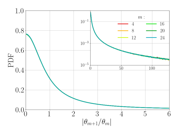
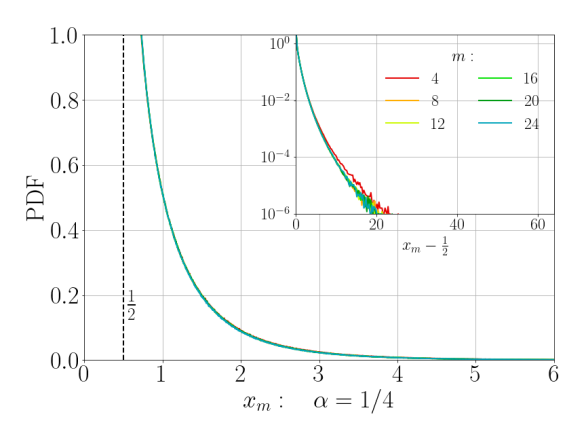
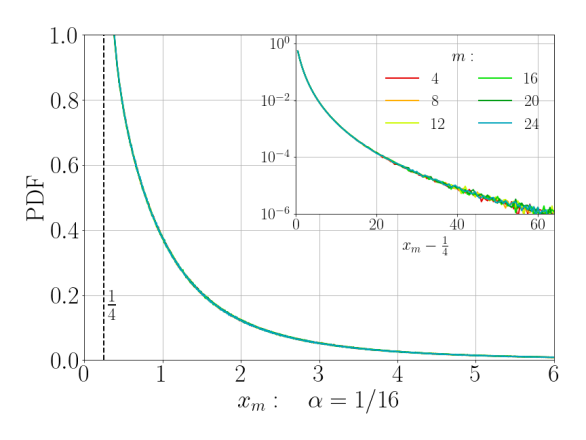
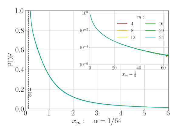
Figure 3: Collapse of PDFs for the multipliers (a) with the standard definition (50) and (b,c,d) with the definition (51) for various values of $\alpha$. Inset uses log scale for the $y$ axis.

More generally, the argument applies for any observable that can be expressed in terms of the rescaled variables. In particular, we later use multipliers defined in terms of the scalar amplitudes as $x_{m}=\mathcal{A}_{m}[\theta]/\mathcal{A}_{m-1}[\theta]$. Using Eqs. (37) and (38) (see Appendix C), these multipliers are expressed as

$$x_{m}(t)=\frac{\mathcal{A}_{m}[\theta(t)]}{\mathcal{A}_{m-1}[\theta(t)]}=\mathcal{X}_{0}[\Theta^{(m)}(\tau^{(m)})],\quad\tau^{(m)}=\gamma^{2m}t,$$ (51)

with the function

$$\mathcal{X}_{0}[\Theta]=\sqrt{\dfrac{\alpha}{1-{\Theta_{0}}^{2}}}\geq\sqrt{\alpha}.$$ (52)

The chief advantage of those new multipliers is that they are constructed as ratios between two strictly positive quantities. Their (single-shell) distributions are given by the pushforward measures $\mathcal{X}_{0\sharp}\mathbb{P}^{(m)}$, whose universality (independence of $m$) is strongly supported by our numerics. Figures 3(b–d) show an accurate collapse of the PDFs, regardless of the specific value of $\alpha$ entering the definition of the scalar amplitudes (37). Similar arguments apply to the universality of joint distributions for multipliers.

V Perron–Frobenius scenario to anomalous scaling laws

The zero-mode analysis of §III highlighted the degeneracy of the scaling symmetry (36), through anomalous power law scalings for the structure functions $\mathcal{S}_{p}$ of orders $p=2$ and $4$. We now intend to address the general case with $p\in\mathbb{R}$. As the averages (20) diverge for large negative orders because of the shell variables accidentally vanishing, we here prefer to work with the moments of scalar amplitudes defined as

$$\Sigma_{p}(\ell_{n})=\lim_{T\to\infty}T^{-1}\int_{0}^{T}\left\langle\mathcal{A}_{m}^{p}[\theta]\right\rangle dt\quad\text{for}\quad p\in\mathbb{R}.$$ (53)

Unlike Eq. (20), we will argue that for suitable values of the parameter $\alpha$ in expression (37), the functions (53) allow to consider negative moments. As such, they prove to be more convenient for both mathematical and numerical analysis. Besides, as shown in Fig. 4(a), the structure functions measured in our numerical experiments demonstrate (anomalous) power-law scalings $\Sigma_{p}(\ell_{n})\propto\ell_{n}^{\xi_{p}}$, in the inertial interval for both positive and negative orders $p$. For positive orders, we have $\xi_{p}=\zeta_{p}$, coinciding with the scaling exponents of the usual moments (20) shown in Fig. 1(b). This identification will be discussed in §VI. In this section, we show that the power-law scalings with anomalous exponents follow from the statistical hidden symmetry, emerging as a suitably defined Perron-Frobenius mode.

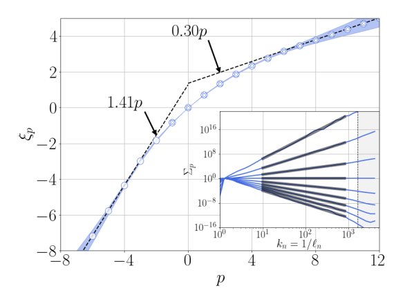
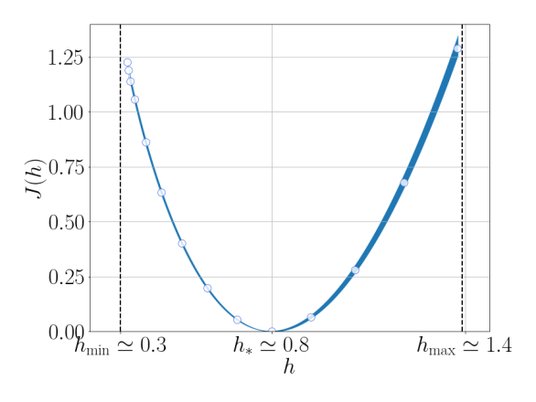
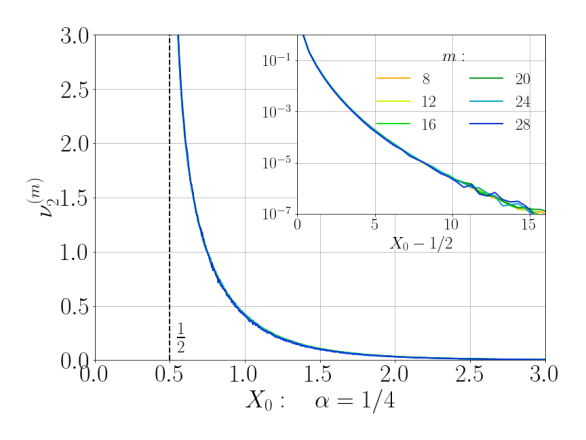
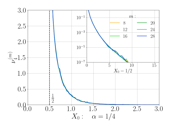
Figure 4: (a) The scaling exponents $\xi_{p}$ for the structure function (53) based on scalar amplitudes with $\alpha=1/4$, indicated with white dots. The white crosses indicate the exponents $\zeta_{p}$ for the usual structure functions from Fig. 1. Insets show the scaling laws for even values of $p$ from $p=-6$ (top) to $p=10$ (bottom). (b) The corresponding rate function $J(h)$. (c,d) Collapse of marginal measure $\nu^{(m)}_{p}$ from Eq. (66) for respectively $p=2$ and $p=4$.

V.1 Structure functions as iterated measures on multipliers

In this subsection, we give a technical derivation showing that the computation of structure functions reduces to an iteration procedure, mediated by linear operators determined by the hidden-symmetry transformation. To that end, we observe that the scalar amplitude is nothing but the telescopic product of multipliers (51):

$$\mathcal{A}_{m}[\theta(t)]=A_{0}\prod_{n=1}^{m}x_{n}(t),$$ (54)

with the constant prefactor $A_{0}=\mathcal{A}_{0}[\theta]=1/\sqrt{1-\alpha}$. At this point, please observe that the product in Eq. (54) extends way beyond the inertial range of scales, as it involves multipliers within the forcing range at scales $\ell_{n}\sim\ell_{0}$. Hence, one should be careful with the hypothesis of statistically restored hidden symmetry (48): Being restricted to the inertial interval, it does not apply at the level of the scalar amplitude (54). The specific forms (42) of the hidden symmetry shift, which map the rescaled processes $\Theta^{(m)}(\tau^{(m)})$ into $\Theta^{(m\pm 1)}(\tau^{(m\pm 1)})$, are more general. They are the consequences of the definition (38) alone and, therefore, remain valid in the forcing range – see Appendix C for more details.

Iterating the hidden symmetry transform (42) yields $\Theta^{(m+N)}=a^{N}[\Theta^{(m)}]$. Combined with Eq. (51), this prescribes the multipliers $x=(x_{n})_{n\in\mathbb{Z}}$ in terms of the maps as

$$x_{n}=\mathcal{X}_{0}[\Theta^{(m+N)}]=\mathcal{X}_{N}[\Theta^{(m)}],\quad\mathcal{X}_{N}=\mathcal{X}_{0}\circ a^{N},\quad n=m+N.$$ (55)

For simplicity, we dropped the corresponding time arguments as they do not affect time averages and, hence, the statistical properties. The pushforward by the map ${\mathcal{X}}[\Theta]=({\mathcal{X}}_{N}[\Theta])_{N\in\mathbb{Z}}$ defines the probability measure $\mathbb{P}_{{\mathcal{X}}}^{(m)}={\mathcal{X}}_{\sharp}\mathbb{P}^{(m)}$ in the space of infinite-dimensional sequences $X=(X_{N})_{N\in\mathbb{Z}}$ with positive components $X_{N}>0$.

We now use the notation $X_{\ominus}=(X_{0},X_{-1},X_{-2},\ldots)$ for inverse sequences of real positive numbers. As such, $\mathbb{P}_{{\mathcal{X}}}^{(m+1)}(dX_{\ominus})$ denotes the measure $\mathbb{P}_{{\mathcal{X}}}^{(m+1)}$ restricted to the subspace $X_{\ominus}$, which in practice prescribes the joint multiplier statistics $(x_{m},x_{m-1},x_{m-2},\ldots)$. From Eq. (55), we observe that the change $m\mapsto m+1$ reduces to a simple shift $N\mapsto N-1$. As a consequence, using Bayes’ formula defining conditional probabilities [42], the measures $\mathbb{P}_{{\mathcal{X}}}^{(m)}$ and $\mathbb{P}_{{\mathcal{X}}}^{(m-1)}$ obey the recursion relation

$$\mathbb{P}_{{\mathcal{X}}}^{(m)}(dX_{\ominus})=\mathbb{P}_{{\mathcal{X}}}^{(m)}(dX_{0}|X_{-})\,\mathbb{P}_{{\mathcal{X}}}^{(m-1)}(d\tilde{X}_{\ominus}),$$ (56)

where $\tilde{X}_{\ominus}=(\tilde{X}_{0},\tilde{X}_{-1},\ldots)$ with $\tilde{X}_{N}=X_{N-1}$, and $\mathbb{P}_{{\mathcal{X}}}^{(m)}(dX_{0}|X_{-})$ denotes the conditional measure for the first component of the sequence $X_{\ominus}=(X_{0},X_{-})$ with $X_{-}=(X_{-1},X_{-2},\ldots)$.

Using the ergodicity assumption in Eq. (53) with the expressions (54) and (55), we have

$$\Sigma_{p}(\ell_{m})=A_{0}^{p}\,\mathbb{E}_{{\mathcal{X}}}^{(m)}\left(\prod_{N=1-m}^{0}X_{N}^{p}\right)=\int\mu_{p}^{(m)}(dX_{\ominus}),$$ (57)

involving the positive measures $\mu_{p}^{(m)}(dX_{\ominus})$ defined in the space $X_{\ominus}$ as

$$\mu_{p}^{(m)}(dX_{\ominus})=A_{0}^{p}\,\left(\prod_{N=1-m}^{0}X_{N}^{p}\right)\mathbb{P}_{{\mathcal{X}}}^{(m)}(dX_{\ominus}).$$ (58)

We point out that the mesures $\mu_{p}^{(m)}$ are not probability measures as they do not generally have unit mass. Their salient feature is that they obey a recursion relation in $m$, which we now derive.

Using Eq. (58) and expressing the measure from Eq. (56) with $\tilde{X}_{N}=X_{N-1}$ yields

$$\begin{array}[]{rcl}\mu_{p}^{(m)}(dX_{\ominus})&=&\displaystyle X_{0}^{p}\,\mathbb{P}_{{\mathcal{X}}}^{(m)}(dX_{0}|X_{-})\left[A_{0}^{p}\,\left(\prod_{N=2-m}^{0}\tilde{X}_{N}^{p}\right)\mathbb{P}_{{\mathcal{X}}}^{(m-1)}(d\tilde{X}_{\ominus})\right]\\[10.0pt] &=&\displaystyle X_{0}^{p}\,\mathbb{P}_{{\mathcal{X}}}^{(m)}(dX_{0}|X_{-})\,\mu_{p}^{(m-1)}(d\tilde{X}_{\ominus}).\end{array}$$ (59)

In a more compact but equivalent form we write

$$\mu_{p}^{(m)}=\mathcal{L}_{p}^{(m)}[\mu_{p}^{(m-1)}],\quad\mathcal{L}_{p}^{(m)}:\mu(dX_{\ominus})\mapsto X_{0}^{p}\,\mathbb{P}_{{\mathcal{X}}}^{(m)}(dX_{0}|X_{-})\,\mu(d\tilde{X}_{\ominus}),$$ (60)

involving $\mathcal{L}_{p}^{(m)}$ as linear positive operator acting on positive measures $\mu(dX_{\ominus})$. The iterative use of Eq. (60) yields the explicit composition representation

$$\mu_{p}^{(m)}=\mathcal{L}^{(m)}_{p}\circ\mathcal{L}^{(m-1)}_{p}\circ\cdots\circ\mathcal{L}^{(1)}_{p}[\mu_{p}^{(0)}],$$ (61)

where $\mu_{p}^{(0)}(dX_{\ominus})=A_{0}^{p}\,\mathbb{P}_{{\mathcal{X}}}^{(0)}(dX_{\ominus})$ is just the Dirac measure of constant multipliers $x_{n}=X_{N}=1$ for $n=N\leq 0$, as prescribed by the (large-scale) boundary conditions in Eq. (3).

V.2 Scaling exponents as Perron–Frobenius eigenvalues

As we already mentioned, the statistical recovery of hidden symmetry (48) cannot be applied directly to the measures $\mu_{p}^{(m)}$ from Eq. (58), because these measures depend on the large-scale statistics of the forcing range. Instead, we use the statistical recovery of hidden symmetry for the linear operators (60), which depend only on the conditional measure $\mathbb{P}_{{\mathcal{X}}}^{(m)}(dX_{0}|X_{-})$. Indeed, this conditional measure is restricted to the inertial interval provided that the shell $m$ belongs to the inertial interval and the correlations of multipliers are local. Therefore, within the inertial interval we have the asymptotic relation

$$\mathcal{L}^{(m)}_{p}=\mathcal{L}^{\infty}_{p},\quad\mathcal{L}_{p}^{\infty}:\mu(dX_{\ominus})\mapsto X_{0}^{p}\,\mathbb{P}_{{\mathcal{X}}}^{\infty}(dX_{0}|X_{-})\,\mu(d\tilde{X}_{\ominus}),$$ (62)

with the universal (independent of $m$) linear operator $\mathcal{L}^{\infty}_{p}$.

The linear operator $\mathcal{L}_{p}^{\infty}$ is positive in the sense that it maps positive measures to positive measures. It follows that its spectral radius is given by a real positive (Perron–Frobenius) eigenvalue $\lambda_{p}$ satisfying the eigenvalue problem [43, 44]

$$\mathcal{L}_{p}^{\infty}[\nu_{p}]=\lambda_{p}\,\nu_{p}.$$ (63)

Here, the eigenvector $\nu_{p}(dX_{\ominus})$ is a positive measure which we normalize to have unit mass $\int\nu_{p}=1$. Under technical non-degeneracy assumptions (referring to strict positivity and compactness [44, Sec. 19.5]), the Perron-Frobenius eigenvalue $\lambda_{p}$ is larger than the absolute values of all remaining eigenvalues. Combining Eq. (61) with (62) and (63), we conclude that the measures $\mu_{p}^{(m)}$ from the inertial interval (for large shells $m$) have the asymptotic form

$$\mu_{p}^{(m)}=c_{p}\lambda_{p}^{m}\,\nu_{p},$$ (64)

involving a positive coefficient $c_{p}$ independent of $m$. Substituting expression (64) into (57), we obtain asymptotic power laws for the structure functions as

$$\Sigma_{p}(\ell_{m})=c_{p}\lambda_{p}^{m}=c_{p}\left(\frac{\ell_{m}}{\ell_{0}}\right)^{\xi_{p}},\quad\xi_{p}=-\log_{\lambda}\lambda_{p},$$ (65)

where we expressed $\ell_{m}/\ell_{0}=\lambda^{-m}$. The scaling exponent is now obtained explicitly in terms of the Perron–Frobenius eigenvalue. This relation allows (and yields in general) a nonlinear dependence of the exponents $\xi_{p}$ on the order $p$ [10]. In this case, the hidden scale invariance provides anomalous power-law scalings for structure functions, and therefore prescribes the intermittency. We remark that, according to Eq. (61), the pre-factors $c_{p}$ are determined by the large-scale statistics, i.e., by the forcing conditions.

V.3 Numerical verification of the Perron–Frobenius scenario

The convergence (up to a constant prefactor) of the measures $\mu_{p}^{(m)}$ towards an eigenvector measure $\nu_{p}$ in Eq. (64) can be addressed numerically. This provides a further assessment of the statistical hidden scale invariance and the confirmation of the Perron–Frobenius scenario for the anomalous scaling. To that end, we normalize the measure $\mu_{p}^{(m)}(dX_{\ominus})$ to unit mass and introduce the corresponding marginal distribution as

$$\nu_{p}^{(m)}(dX_{0})=\frac{1}{\Sigma_{p}(\ell_{m})}\int_{X_{-}}\mu_{p}^{(m)}(dX_{0},dX_{-}).$$ (66)

The Perron-Frobenius scenario predicts that the measures $\nu_{p}^{(m)}(dX_{0})$ should converge towards the single-shell marginal of the eigenvector $\nu_{p}(dX_{0})$, which by construction has unit mass and is independent of $m$.

From a numerical standpoint, the distribution (66) is estimated as the limit

$$\nu_{p}^{(m)}(dX_{0})=\dfrac{1}{\Sigma_{p}(\ell_{m})}\lim_{T\to\infty}T^{-1}\int_{0}^{T}dt\,\left\langle\mathcal{A}_{m}^{p}[\theta]\mathbbm{1}_{x_{m}(t)\in dX_{0}}\right\rangle,$$ (67)

which stems from the definition (58) combined with the expressions (53) and (55). Outcomes from our numerics are presented in Fig. 4(c,d) for $p=2,4$. Each panel shows the densities for the shells $m=4,\ldots,28$ in the inertial interval. The accurate collapse of the graphs verifies the convergence of the measures $\nu_{p}^{(m)}$ towards a well-identified (Perron-Frobenius) eigenmode and provides strong numerical support to our theory.

VI From Perron-Frobenius to zero-modes and multifractality

This section discusses the implications of the Perron-Frobenius scenario beyond the observation of power-law scaling for the specific structure functions (53), based on the scalar amplitudes. We show that the statistical restoring of hidden symmetry also prescribes: (i) the scaling of usual structure functions $\mathcal{S}_{p}$ with the same exponents, at least for the orders when the time average is well-defined. (ii) the fusion rules required to evidence the zero-mode scenario and (iii) the Parisi–Frisch multifractal formalism.

VI.1 Scaling of the usual structure functions

Through Eq. (64), the Perron-Frobenius scenario predicts power-law scalings for the measures $\mu_{p}^{(m)}$, and hence for any observables that can be associated with these measures. Scalings for the structure functions $\Sigma_{p}$ in Eq. (65) represent just a particular example. We now show that the scalings for usual structure functions $\mathcal{S}_{p}$ from Eq. (20) follow in a similar manner.

Using Eqs. (37), (51) and (54), one obtains the identity

$$|\theta_{m}|=\sqrt{\mathcal{A}_{m}^{2}[\theta]-\alpha\mathcal{A}_{m-1}^{2}[\theta]}=\sqrt{1-\frac{\alpha\mathcal{A}_{m-1}^{2}[\theta]}{\mathcal{A}_{m}^{2}}}\,\mathcal{A}_{m}=\sqrt{1-\frac{\alpha}{x_{m}^{2}}}\,A_{0}\prod_{n=1}^{m}x_{n}.$$ (68)

This expression differs from Eq. (54) only by the square root prefactor depending on $x_{m}$. One can check that this prefactor modifies the expression (57) for the structure function (20) as

$$\mathcal{S}_{p}(\ell_{m})=\int\left(1-\frac{\alpha}{X_{0}^{2}}\right)^{p/2}\mu_{p}^{(m)}(dX_{\ominus}).$$ (69)

Finally, using the Perron–Frobenius asymptotic relation (64), we obtain

$$\mathcal{S}_{p}(\ell_{m})=\tilde{c}_{p}\left(\frac{\ell_{m}}{\ell_{0}}\right)^{\xi_{p}},\quad\tilde{c}_{p}=c_{p}\int\left(1-\frac{\alpha}{X_{0}^{2}}\right)^{p/2}\,\nu_{p}(dX_{\ominus}),$$ (70)

involving the same exponent $\xi_{p}=-\log_{\lambda}\lambda_{p}$ but a different prefactor $\tilde{c}_{p}$. Naturally, the relation (70) is meaningful only provided that the integral in the second expression converges. For the structure functions $\mathcal{S}_{p}$, the divergence is expected for negative orders $p\leq 1$ due to accidental zeros of shell variables. Our numerics supports this scenario: for $p>-1$, the exponents $\zeta_{p}=\xi_{p}$, meaning that the scaling exponents of $\mathcal{S}_{p}$ and $\Sigma_{p}$ coincide. Figure 4(a) shows that both families share the same asymptotic behavior

$$\xi_{p}=\zeta_{p}\sim 0.3p\quad\textrm{as}\quad p\to+\infty.$$ (71)

Divergence are seen for $p\leq-1$: The usual structure functions $\mathcal{S}_{p}$ diverge while their scalar amplitude counterparts of Fig. 4(a) are well-behaved, with the apparent asymptotic

$$\xi_{p}\sim 1.4p\quad\textrm{as}\quad p\to-\infty.$$ (72)

VI.2 Fusion rules

The hidden scaling symmetry determines the fusion rules formulated for the fourth-order correlators by Eq. (30). It is sufficient to prove that

$$\sigma_{m(-l)}=C_{-l}\sigma_{m0}\quad\textrm{for}\quad l\geq 0.$$ (73)

Indeed, relation (73) yields Eq. (30) with a different sign of $l$ as

$$\sigma_{nl}=\sigma_{(n+l)(-l)}=C_{-l}\sigma_{(n+l)0}=C_{-l}\lambda^{-\zeta_{4}l}\sigma_{n0}=C_{l}\sigma_{n0},\quad C_{l}=C_{-l}\lambda^{-\zeta_{4}l},$$ (74)

where we also used Eqs. (24) and (29). Using Eq. (68) for $m$ and $m-l$, we express

$$\theta_{m}^{2}\theta_{m-l}^{2}=\left(1-\frac{\alpha}{x_{m}^{2}}\right)\left(1-\frac{\alpha}{x_{m-l}^{2}}\right)\left(\prod_{j=m-l+1}^{m}x_{j}^{-2}\right)\mathcal{A}_{m}^{4}[\theta].$$ (75)

As in the previous subsection, one can check that the average of function (75) yields the expression analogous to Eq. (57) but with the modified prefactor as

$$\sigma_{m(-l)}=\int\left(1-\frac{\alpha}{X_{0}^{2}}\right)\left(1-\frac{\alpha}{X_{-l}^{2}}\right)\left(\prod_{j=0}^{l-1}X_{-j}^{-2}\right)\mu_{4}^{(m)}(dX_{\ominus}).$$ (76)

Using the Perron-Frobenius representation (64), we find

$$\sigma_{m(-l)}=\hat{c}_{l}\left(\frac{\ell_{m}}{\ell_{0}}\right)^{\xi_{4}},\quad\hat{c}_{l}=c_{4}\int\left(1-\frac{\alpha}{X_{0}^{2}}\right)\left(1-\frac{\alpha}{X_{-l}^{2}}\right)\left(\prod_{j=0}^{l-1}X_{-j}^{-2}\right)\nu_{4}(dX_{\ominus}).$$ (77)

This expression yields the fusion rules (30) with the coefficients $C_{l}=\hat{c}_{l}/\hat{c}_{0}$. Thus, the practical implementation of the zero-mode theory follows from the Perron–Frobenius scenario and the statistical recovery of hidden scale invariance.

VI.3 Multifractal formalism

The multiplicative representation of the scalar amplitudes (54) and the Perron-Frobenius scenario for intermittency provide an explicit multifractal interpretation of the scaling exponents through large deviations, in particular the Gärtner–Ellis Theorem [45]. For positive $m$, let us define the effective Hölder exponents as the sample mean

$$H_{m}=-\dfrac{1}{m}\sum_{J=0}^{m-1}\log_{\lambda}X_{-J},$$ (78)

where $X_{0},X_{-1},\ldots$ are random numbers with the probability distribution $\mathbb{P}_{\mathcal{X}}^{(m)}$. It follows from Eqs. (54) and (55) that $H_{m}=h$ identifies to the monofractal asymptotics $\mathcal{A}_{m}=A_{0}\lambda^{-mh}$. Besides, the characteristic function of $H_{m}$ recovers the structure functions through the following calculation

$$\mathbb{E}_{\mathcal{X}}^{(m)}\left[A_{0}^{p}\lambda^{-mpH_{m}}\right]=\Sigma_{p}(\ell_{m})\sim c_{p}\lambda^{-m\xi_{p}},\quad m\to\infty,$$ (79)

with the second equality stemming from the Perron-Frobenius identity (65). In other words, the Perron-Frobenius scenario provides existence of the generating function

$$p\mapsto-\lim_{m\to\infty}\dfrac{1}{m}\log_{\lambda}\mathbb{E}_{\mathcal{X}}^{(m)}\left[\lambda^{-mpH_{m}}\right]=\xi_{p},\quad p\in\mathbb{R}.$$ (80)

Further assuming that the generating function is smooth for all real orders $p$, the Gärtner–Ellis Theorem [45, 12] yields the large deviation estimate valid for $m\to\infty$ as

$$\mathbb{P}_{\mathcal{X}}^{(m)}\left(H_{m}\in dh\right)\approx\lambda^{-mJ(h)}dh$$ (81)

with the rate function

$$J(h)=\sup_{p\in\mathbb{R}}\,(\xi_{p}-ph).$$ (82)

In the multifractal language [1, 8], $J(h)$ plays the role of fractal codimension. So, the fractal dimension (singularity spectrum) is defined as $D(h)=d-J(h)$, where $d$ is the dimension of physical space. In turn, the scaling exponents are expressed through the Legendre–Fenschel transform as

$$\xi_{p}=\inf_{h\in\mathbb{R}}\,\left[ph+J(h)\right].$$ (83)

Equations (78), (81) and (83) summarize the multifractal theory as a large deviation principle stemming from the statistically recovery of the hidden symmetry.

From a numerical viewpoint, we infer from Fig. 4(a) that the function $\xi_{p}$ is apparently smooth and concave on $\mathbb{R}$ with linear asymptotics (71) and (72). It follows from classical properties of the Legendre–Fenschel transforms [46], that the rate function is convex and compactly supported on

$$h_{\min}\leq h\leq h_{\max},\quad h_{\min}\approx 0.3,\quad h_{\max}\approx 1.4,$$ (84)

with vertical asymptotics at $h_{\min}$ and $h_{\max}$ – see Fig. 4(b). As a final comment, please observe that the exponent $h_{\max}$ prescribes the steepest rate of decay for the scalar amplitudes as

$$|\theta_{m}|\sim\mathcal{A}_{m}[\theta]\propto\lambda^{-mh_{\max}}.$$ (85)

It follows that the sums with respect to $n$, which appear in Eq. (37) and other similar expressions, converge exponentially in the inertial interval for any $\alpha<\lambda^{-2h_{\max}}$. In the numerics presented here, we have $\lambda^{-2h_{\max}}\approx 0.52$. This (finally!) substantiates the choices of $\alpha$ used in all our derivations and simulations.

VII Concluding remarks

By revisiting a simple model of random scalar advection, we contrasted two apparently distinct generic scenarios for spatial intermittency: zero-mode vs Perron-Frobenius associated to (hidden) statistical scale invariance. The zero-mode scenario evidences anomalous power-law scalings for even-order structure functions through a direct, exact computation, whose success owes to two specific ingredients: the presence of non-trivial statistical conservation laws and power-law decays for two-shell correlators, implemented in the form of a fusion rule ansatz. Neither of the two ingredients are unique to the KWB dynamics under consideration [33]: duality between zero-mode and statistical conservation laws is a hallmark feature of passive scalar dynamics [26], and fusion-like rules are expected to hold in a variety of settings [47, 48, 49, 50, 51]. Besides, numerical studies suggest the presence of zero-modes beyond the case of random advection in Gaussian Markov environments [40, 52]. Yet, their explicit computation pose increasing difficulties in more sophisticated settings, including but not limited to addressing finite space-dimensionality [53], non-Markov [32, 33, 54] or non-gaussian advection [55], quenched statistics [54], and nonlinearities [56].

By contrast, the Perron-Frobenius scenario relies on statistical symmetries obtained from the dynamical rescaling of the original scalar dynamics. While the rescaled dynamics is not linear any longer, what matters is that it possesses a weaker form of scale invariance: the hidden scale invariance, which we can evidence through statistical observations. Stricto sensu, our approach is not computational as is does not prescribe analytic values for the various exponents. Practical outcomes of our approach however include (i) universality of multiplier statistics and generalized ratios, (ii) explicit connection between anomalous scaling and joint spatial statistics of multipliers, (iii) derivation of fusion-rule ansatz required for the zero-mode computation, (iv) substantiation of the multifractal formalism. As such, the Perron-Frobenius scenario fully determines the spatial intermittency. We point out that the scenario does not not crucially depend on the specificity of the KWB dynamics, in particular its random nature and its linearity. In fact, and unlike the zero-mode scenario, the Perron-Frobenius does not rely on the specific details of the dynamics but rather on its symmetries and nonlinearities. The fact that universality of multipliers is observed throughout fluid models, from the present KWB dynamics and shell models [15, 16, 18] to direct simulations of fluid equations [11] and experiments [14], strongly suggests not only that the Perron-Frobenius scenario is a generic mechanism behind fluid intermittency in fluid flows, but also that it can be evidenced in a systematic fashion. Let us here point out that the hidden KWB system (40) shares a structural analogy with the rescaled ideal systems obtained for non-linear shell models and the Navier-Stokes equations [10, 18, 11], which can be traced back to structural analogies in the underlying dynamics. Besides, while the hidden symmetry here discussed is limited to the inertial range of scales, extensions to include the diffusion range are possible, following the ideas developed in [12] for turbulence models.

Compared to real flows, the model considered in this paper combines several simplifying features: lack of Galilean symmetry coming from the shell-model setting, and lack of intermittency for the carrier flow. Such features can be accomodated in the hidden symmetry framework using slightly different rescaling strategies [10, 11]. Natural extensions of this work include, but are not limited to, explicit address of real-space scalar intermittency in various types of advecting environments, implications of hidden symmetry on multi-scale and multi-time correlators, and derivation of associated fusion rules.

Appendix A Itô  calculus for structure functions

Here we derive equations for the second and fourth order structure functions. The mutually independent Wiener processes $(w_{n})_{n\in\mathbb{Z}}$ prescribe the fundamental property $dw_{i}dw_{i}=\delta_{ij}dt$ [57, 37, 42]. Hence, using definition (9), we derive

$$\mathcal{N}_{n}[\theta,dw]\,\mathcal{N}_{n-j}[\theta,dw]=\mathcal{C}_{n(n-j)}[\theta]\,dt,\quad\mathcal{C}_{n(n-j)}[\theta]=\begin{cases}\gamma^{2n}\left(\theta_{n+1}^{2}+\gamma^{-2}\theta_{n-1}^{2}\right),&j=0;\\ -\gamma^{2n-2}\theta_{n}\theta_{n-1},&j=1;\\ 0,&j>1.\end{cases}$$ (86)

For the function $\theta_{n}^{2}$ with $n=1,\ldots,n_{\max}$, Itô’s lemma [37] with Eq. (8) yields

$$d\theta_{n}^{2}=2\theta_{n}\mathcal{N}_{n}[\theta,dw]+2\left(I_{n}+B_{n}-D_{n}\right)\theta_{n}^{2}\,dt+\mathcal{C}_{nn}[\theta]\,dt,$$ (87)

Let us average this equation over random realizations of the Wiener processes $w=(w_{n})_{n\in\mathbb{Z}}$. The term $\left\langle\theta_{n}\mathcal{N}_{n}[\theta,dw]\right\rangle$ vanishes, because $\theta$ and $dw$ are mutually independent in Itô  calculus. In the remaining terms, we substitute the coefficients from Eq. (10), the expression for $\mathcal{C}_{nn}[\theta]$ from Eq. (86), and use boundary conditions (3). One can check that the resulting expression yields the scalar energy balance Eqs. (11) and (12).

Now, let us perform a similar analysis for any scalar function $\mathcal{F}[\theta]$. We assume that $\mathcal{F}[\theta]$ depends smoothly on shell scalars $\theta_{n}$ governed by the ideal model (16). Taking into account that $\mathcal{C}_{n(n-j)}[\theta]\equiv 0$ for $j>1$ in Eq. (86), by Itô’s lemma [37] we have

$$d\mathcal{F}[\theta]=\sum_{j\in\mathbb{Z}}\left(\frac{\partial\mathcal{F}}{\partial\theta_{j}}\,d\theta_{j}+\frac{1}{2}\frac{\partial^{2}\mathcal{F}}{\partial\theta_{j}^{2}}\,\mathcal{C}_{jj}[\theta]\,dt+\frac{\partial^{2}\mathcal{F}}{\partial\theta_{j}\partial\theta_{j-1}}\,\mathcal{C}_{j(j-1)}[\theta]\,dt\right),\quad d\theta_{j}=\mathcal{N}_{j}[\theta,dw]+I_{j}\theta_{j}\,dt.$$ (88)

Let us average Eq. (88) over random realizations of $w$. Then the terms containing $\mathcal{N}_{j}[\theta,dw]$ vanish, and the remaining terms yield

$$\frac{d}{dt}\left\langle\mathcal{F}[\theta]\right\rangle=\left\langle\mathcal{L}\left[\mathcal{F}\right]\right\rangle,\quad\mathcal{L}[\mathcal{F}]:=\sum_{j\in\mathbb{Z}}\frac{\partial\mathcal{F}}{\partial\theta_{j}}\,I_{j}\theta_{j}+\frac{1}{2}\frac{\partial^{2}\mathcal{F}}{\partial\theta_{j}^{2}}\,\mathcal{C}_{jj}[\theta]+\frac{\partial^{2}\mathcal{F}}{\partial\theta_{j}\partial\theta_{j-1}}\,\mathcal{C}_{j(j-1)}[\theta].$$ (89)

The functionnal $\mathcal{L}$ represents the (infinitesimal) generator of the scalar dynamics. Equations for two-shell functions follow by taking $\mathcal{F}[\theta]=\theta^{2}_{n}\theta^{2}_{n+l}$ in Eq. (89). Elementary computations yield

$$\dfrac{d}{dt}\left\langle\theta_{n}^{2}\theta_{n+l}^{2}\right\rangle=\left\langle 2(I_{n}+I_{n+l})\theta_{n}^{2}\theta_{n+l}^{2}\right\rangle+\left\{\begin{array}[]{ll}6\left\langle\theta_{n}^{2}\mathcal{C}_{nn}[\theta]\right\rangle,&l=0;\\ 4\left\langle\theta_{n}\theta_{n+1}\mathcal{C}_{(n+1)n}[\theta]\right\rangle,&l=1;\\ \left\langle\theta_{n+l}^{2}\mathcal{C}_{nn}[\theta]+\theta_{n}^{2}\mathcal{C}_{(n+l)(n+l)}[\theta]\right\rangle,&l\geq 2.\\ \end{array}\right.$$ (90)

Substituting $I_{n}$ from Eq. (10), one obtains Eqs. (25) and (26).

Appendix B Derivation of the hidden KWB system

In this section, we provide the detailed derivation of rescaled system (40) from the ideal model Eq. (16). For simplicity, we drop the superscript $(m)$ through this section.

Using expressions (37) and (38) for given $N$, we introduce the function $\mathcal{F}[\theta]$ as

$$\Theta_{N}=\mathcal{F}[\theta]:=\frac{\theta_{m+N}}{\mathcal{A}_{m}[\theta]},\quad\mathcal{A}_{m}[\theta]=\sqrt{\sum_{n\leq m}\alpha^{m-n}\theta_{n}^{2}}.$$ (91)

Our intention is to use Eq. (88). For the first derivatives, one computes

$$\frac{\partial\mathcal{F}}{\partial\theta_{j}}=\frac{\mathbbm{1}_{j=m+N}}{\mathcal{A}_{m}[\theta]}-\frac{\alpha^{m-j}\theta_{m+N}\theta_{j}}{\mathcal{A}_{m}^{3}[\theta]}\,\mathbbm{1}_{j\leq m}.$$ (92)

Considering $N>1$, for the second derivatives we have

$$\frac{\partial^{2}\mathcal{F}}{\partial\theta_{j}^{2}}=-\frac{2\alpha^{m-j}\theta_{j}}{\mathcal{A}_{m}^{3}[\theta]}\,\mathbbm{1}_{j=m+N\leq m}+\frac{\alpha^{m-j}\theta_{m+N}}{\mathcal{A}_{m}^{3}[\theta]}\left(\frac{3\alpha^{m-j}\theta_{j}^{2}}{\mathcal{A}_{m}^{2}[\theta]}-1\right)\mathbbm{1}_{j\leq m},$$ (93)

$$\frac{\partial^{2}\mathcal{F}}{\partial\theta_{j}\partial\theta_{j-1}}=-\frac{\alpha^{m-j+1}\theta_{j-1}}{\mathcal{A}_{m}^{3}[\theta]}\,\mathbbm{1}_{j=m+N\leq m+1}-\frac{\alpha^{m-j}\theta_{j}}{\mathcal{A}_{m}^{3}[\theta]}\,\mathbbm{1}_{j=m+N+1\leq m}+\frac{3\alpha^{2m-2j+1}\theta_{m+N}\theta_{j}\theta_{j-1}}{\mathcal{A}_{m}^{5}[\theta]}\,\mathbbm{1}_{j\leq m}.$$ (94)

Substituting Eqs. (92)–(94) into (88), after elementary manipulations we have

$$\begin{split}&d\Theta_{N}=d\mathcal{F}[\theta]=\frac{d\theta_{m+N}}{\mathcal{A}_{m}[\theta]}-\sum_{j\leq m}\alpha^{m-j}\frac{\theta_{m+N}\theta_{j}}{\mathcal{A}_{m}^{2}[\theta]}\frac{d\theta_{j}}{\mathcal{A}_{m}[\theta]}\\[7.0pt] &-\alpha^{-N}\frac{\theta_{m+N}}{\mathcal{A}_{m}[\theta]}\frac{\mathcal{C}_{(m+N)(m+N)}[\theta]}{\mathcal{A}_{m}^{2}[\theta]}\,dt\,\mathbbm{1}_{N\leq 0}+\frac{1}{2}\sum_{j\leq m}\alpha^{m-j}\frac{\theta_{m+N}}{\mathcal{A}_{m}[\theta]}\left(3\alpha^{m-j}\frac{\theta_{j}^{2}}{\mathcal{A}_{m}^{2}[\theta]}-1\right)\frac{\mathcal{C}_{jj}[\theta]}{\mathcal{A}_{m}^{2}[\theta]}\,dt\\[7.0pt] &-\alpha^{-N+1}\frac{\theta_{m+N-1}}{\mathcal{A}_{m}[\theta]}\frac{\mathcal{C}_{(m+N)(m+N-1)}[\theta]}{\mathcal{A}_{m}^{2}[\theta]}\,dt\,\mathbbm{1}_{N\leq 1}-\alpha^{-N-1}\frac{\theta_{m+N+1}}{\mathcal{A}_{m}[\theta]}\frac{\mathcal{C}_{(m+N+1)(m+N)}[\theta]}{\mathcal{A}_{m}^{2}[\theta]}\,dt\,\mathbbm{1}_{N\leq-1}\\[7.0pt] &+\sum_{j\leq m}3\alpha^{2m-2j+1}\frac{\theta_{m+N}\theta_{j}\theta_{j-1}}{\mathcal{A}_{m}^{3}[\theta]}\frac{\mathcal{C}_{j(j-1)}[\theta]}{\mathcal{A}_{m}^{2}[\theta]}\,dt.\end{split}$$ (95)

Using expressions (38) and (86), one writes

$$\frac{\mathcal{C}_{jj}[\theta]}{\mathcal{A}_{m}^{2}[\theta]}\,dt=\gamma^{2J}\left(\Theta_{J+1}^{2}+\gamma^{-2}\Theta_{J-1}^{2}\right)d\tau,\quad\frac{\mathcal{C}_{j(j-1)}[\theta]}{\mathcal{A}_{m}^{2}[\theta]}\,dt=-\gamma^{2J-2}\Theta_{J}\Theta_{J-1}d\tau,\quad j=m+J.$$ (96)

Similarly, using expressions (38), (16), (9) and (10), we derive

$$\frac{d\theta_{j}}{\mathcal{A}_{m}[\theta]}=\mathcal{N}_{J}[\Theta,dW]+I_{J}\Theta_{J}d\tau,\quad j=m+J.$$ (97)

Substituting Eqs. (96) and (97) into (95), using expressions (38) and changing the summation index as $J=j-m$ yields

$$\begin{split}d\Theta_{N}=&\,\mathcal{N}_{N}[\Theta,dW]+I_{N}\Theta_{N}d\tau-\Theta_{N}\sum_{J\leq 0}\alpha^{-J}\Theta_{J}\left(\mathcal{N}_{J}[\Theta,dW]+I_{J}\Theta_{J}d\tau\right)\\[3.0pt] &-\alpha^{-N}\Theta_{N}\gamma^{2N}\left(\Theta_{N+1}^{2}+\gamma^{-2}\Theta_{N-1}^{2}\right)d\tau\,\mathbbm{1}_{N\leq 0}\\[3.0pt] &+\alpha^{-N+1}\gamma^{2N-2}\Theta_{N}\Theta_{N-1}^{2}d\tau\,\mathbbm{1}_{N\leq 1}+\alpha^{-N-1}\gamma^{2N}\Theta_{N+1}^{2}\Theta_{N}d\tau\,\mathbbm{1}_{N\leq-1}\\[3.0pt] &+\Theta_{N}\sum_{J\leq 0}\left[\frac{\alpha^{-J}}{2}(3\alpha^{-J}\Theta_{J}^{2}-1)\gamma^{2J}(\Theta_{J+1}^{2}+\gamma^{-2}\Theta_{J-1}^{2})-3\alpha^{1-2J}\gamma^{2J-2}\Theta_{J}^{2}\Theta_{J-1}^{2}\right]d\tau.\end{split}$$ (98)

Equation (98) is the Itô  version of the hidden KWB dynamics (40). It is recovered from Eqs. (40) and (41) by expanding to order $d\tau$ the following practical Stratonovich-Itô  conversion formula [42]

$$\circ\Lambda_{N}\left[\Theta,{\mathcal{N}}\left[\Theta,dW\right]\right]=\Lambda_{N}\left[\Theta+\frac{d\Theta}{2},{\mathcal{N}}\left[\Theta+\frac{d\Theta}{2},dW\right]\right],$$ (99)

yielding

$$\circ\Lambda_{N}[\Theta,\mathcal{N}]=\Lambda_{N}[\Theta,{\mathcal{N}}+I\Theta d\tau]-{\mathcal{N}}_{N}d\mathcal{A}\left[\Theta,{\mathcal{N}}\right]+\dfrac{\Theta_{N}}{2}\Big{(}3\left(d\mathcal{A}\left[\Theta,{\mathcal{N}}\right]\right)^{2}-d\mathcal{A}\left[{\mathcal{N}},{\mathcal{N}}\right]\Big{)}$$ (100)

with the shorthands

$${\mathcal{N}}:=\mathcal{N}[\Theta,dW],\quad d\mathcal{A}[V,W]:=\sum_{J\leq 0}\alpha^{-J}V_{J}W_{J}.$$ (101)

The first right-hand side term in Eq. (100) provides the first line in Eq. (98). The remaining terms are generalized Itô  terms, which upon using Eq. (86), precisely yield the remaining lines in Eq. (98). This completes the derivation of the Hidden KWB dynamics (40).

Appendix C Derivation of hidden symmetry transformation

Here we prove that relations (42) and (43) map the processes $\Theta^{(m)}(\tau^{(m)})$ and $W^{(m)}(\tau^{(m)})$ into $\Theta^{(m\pm 1)}(\tau^{(m\pm 1)})$ and $W^{(m\pm 1)}(\tau^{(m\pm 1)})$. These processes satisfy equations of the same rescaled system (40), which is independent of $m$. Therefore, it follows that the transformations (42) induce a group of symmetries of the rescaled equations.

One can deduce relations (42) and (43) for $W$ and $\tau$ directly from Eq. (38) considered for $m$ and $m\pm 1$. It remains to show that the operators $a^{\pm 1}$ map $\Theta^{(m)}$ into $\Theta^{(m\pm 1)}$. Let us first consider the case of positive sign. Using (37), we write

$$\mathcal{A}_{m+1}[\theta]=\sqrt{\theta_{m+1}^{2}+\alpha\theta_{m}^{2}+\alpha^{2}\theta_{m-1}^{2}+\cdots}=\sqrt{\theta_{m+1}^{2}+\alpha\mathcal{A}_{m}^{2}[\theta]}=\mathcal{A}_{m}[\theta]\sqrt{\left(\Theta_{1}^{(m)}\right)^{2}+\alpha},$$ (102)

where we expressed $\Theta_{1}^{(m)}=\theta_{m+1}/\mathcal{A}_{m}[\theta]$ in the last equality from Eq. (38). Using Eq. (102) in (38), we write

$$\Theta_{N}^{(m+1)}=\frac{\theta_{m+N+1}}{\mathcal{A}_{m+1}[\theta]}=\frac{\theta_{m+N+1}}{\mathcal{A}_{m}[\theta]\sqrt{\Theta_{1}^{2}+\alpha}}=\frac{\Theta_{N+1}^{(m)}}{\sqrt{\alpha+\left(\Theta_{1}^{(m)}\right)^{2}}},$$ (103)

which yields the first relation in Eq. (43). Similarly, for the negative sign, we have

$$\mathcal{A}_{m-1}[\theta]=\sqrt{\theta_{m-1}^{2}+\alpha\theta_{m-2}^{2}+\cdots}=\sqrt{(\mathcal{A}_{m}^{2}[\theta]-\theta_{m}^{2})/\alpha}=\mathcal{A}_{m}[\theta]\sqrt{\frac{1-\left(\Theta_{0}^{(m)}\right)^{2}}{\alpha}}.$$ (104)

Then we derive the second relation in Eq. (43) as

$$\Theta_{N}^{(m-1)}=\frac{\theta_{m+N-1}}{\mathcal{A}_{m-1}[\theta]}=\frac{\theta_{m+N-1}}{\mathcal{A}_{m}[\theta]}\sqrt{\frac{\alpha}{1-\left(\Theta_{0}^{(m)}\right)^{2}}}=\sqrt{\frac{\alpha}{1-\left(\Theta_{0}^{(m)}\right)^{2}}}\,\Theta_{N-1}^{(m)}.$$ (105)

Appendix D Zero modes as statistical conservation laws

We here point out that the zero-modes solving the eigenvalue problems (23) and (28) relate to the presence of explicit statistical conservations laws, which we respectively label as $\Gamma_{2}$ and $\Gamma_{4}$.

D.1 The $\Gamma_{2}$ invariant

Let us show that the Kolmogorov zero-mode $\mathcal{S}_{2}(\ell_{n})=\gamma^{-2n}$ solving Eq. (23) is dual to the ideal conservation of the statistical invariant

$$\Gamma_{2}:=\sum_{n\in\mathbb{Z}}\gamma^{-2n}\left\langle\theta_{n}^{2}\right\rangle.$$ (106)

The ideal conservation of $\Gamma_{2}$ associated to Eq. (17) is seen from the direct telescopic calculation

$$\dfrac{d}{dt}\Gamma_{2}=\sum_{n\in\mathbb{Z}}\left(\gamma^{-2}\left\langle\theta_{n-1}^{2}\right\rangle-(\gamma^{-2}+1)\left\langle\theta_{n}^{2}\right\rangle+\left\langle\theta_{n+1}^{2}\right\rangle\right)=0,$$ (107)

where the last equality follows after the formal change of indices $n\pm 1\mapsto n$. More fundamentally, let us write Eq. (17) as

$$\dfrac{d\left\langle\theta_{n}^{2}\right\rangle}{dt}=\sum_{n^{\prime}\in\mathbb{Z}}M_{nn^{\prime}}\left\langle\theta_{n^{\prime}}^{2}\right\rangle$$ (108)

with the matrix elements

$$M_{nn^{\prime}}=\gamma^{2n-2}\delta_{(n-1)n^{\prime}}-\left(\gamma^{2n-2}+\gamma^{2n}\right)\delta_{nn^{\prime}}+\gamma^{2n}\delta_{(n+1)n^{\prime}}.$$ (109)

The stationary solution $\left\langle\theta_{n}^{2}\right\rangle=\gamma^{-2n}$ is a right zero-mode of $M$, i.e. $\sum_{n^{\prime}\in\mathbb{Z}}M_{nn^{\prime}}\gamma^{-2n^{\prime}}=0$ for all $n\in\mathbb{Z}$. Notice that the matrix $M=(M_{nn^{\prime}})$ is symmetric. Hence, the ideal conservation of $\Gamma_{2}$ given by Eq. (106) follows from the observation that $\gamma^{-2n}$ is also a left zero-mode, i.e. $\sum_{n\in\mathbb{Z}}\gamma^{-2n}M_{nn^{\prime}}=0$ for all $n^{\prime}\in\mathbb{Z}$. In that sense, the ideal statistical conservation of $\Gamma_{2}$ is dual to the Kolmogorov scaling $\mathcal{S}_{2}(\ell_{n})=\gamma^{-2n}$.

D.2 The $\Gamma_{4}$ invariant.

The same type of duality holds for the fourth-order zero-mode: $\sigma_{nl}=C_{l}S_{4}(\ell_{n})$ with $S_{4}(\ell_{n})\propto\ell^{\zeta_{4}}$ from Section III.2. This zero-mode ties to the statistical conservation of the quantity

$$\Gamma_{4}=\sum_{n}g_{n},\quad g_{n}:=\sum_{l\geq 0}c_{l}r^{n}\left\langle\theta_{n}^{2}\theta_{n+l}^{2}\right\rangle,$$ (110)

where $c_{l}=6C_{l}-5\delta_{l0}$ and $r=\lambda^{-\zeta_{4}}$. This conservation law can be expressed in the form

$$\dfrac{d}{dt}g_{n}=\Pi^{g}_{n-1}-\Pi^{g}_{n},$$ (111)

where some straightforward but tedious algebra (see the next §D.3) yields the flux as

$$\Pi^{g}_{n}=\sum_{l\geq 0}\pi^{g}_{ln},\quad\pi^{g}_{ln}:=\begin{cases}-\left(r\gamma^{2}\right)^{n}\left\langle\theta_{n+1}^{4}\right\rangle,&l=0;\\ \left(r\gamma^{2}\right)^{n}\left(c_{2}\left\langle\theta_{n+1}^{2}\theta_{n+2}^{2}\right\rangle-6r\left\langle\theta_{n}^{2}\theta_{n+1}^{2}\right\rangle\right),&l=1;\\ \left(r\gamma^{2}\right)^{n}\left(c_{l+1}\left\langle\theta_{n+1}^{2}\theta_{n+l+1}^{2}\right\rangle-c_{l-1}r\left\langle\theta_{n}^{2}\theta_{n+l}^{2}\right\rangle\right),&l\geq 1.\end{cases}$$ (112)

The dual origin of the invariant $\Gamma_{4}$ can be seen by writing Eq. (25) as

$$\begin{split}\gamma^{-2n-l}\dfrac{d}{dt}\left\langle\theta^{2}_{n}\theta^{2}_{n+l}\right\rangle=\sum_{n^{\prime},l^{\prime}}{\mathcal{M}}_{nl,n^{\prime}l^{\prime}}\left\langle\theta^{2}_{n^{\prime}}\theta^{2}_{n^{\prime}+l^{\prime}}\right\rangle.\end{split}$$ (113)

Here the right-hand side vanishes for the fourth-order zero-mode solution $\left\langle\theta_{n}^{2}\theta_{n+l}^{2}\right\rangle=\sigma_{nl}$ given by Eq. (28). Let $\tilde{\sigma}_{nl}$ be the corresponding left zero-mode satisfying the equation $\sum_{n,l}\tilde{\sigma}_{nl}{\mathcal{M}}_{nl,n^{\prime}l^{\prime}}=0$ for all $n^{\prime}$ and $l^{\prime}$. One can show that the left zero-mode is found explicitly as $\gamma^{-2n-l}\tilde{\sigma}_{nl}=\left(6-5\delta_{l0}\right)\sigma_{nl}=c_{l}r^{n}$. This dual zero-mode yields the conservation law for $\Gamma_{4}$ in Eq. (110).

D.3 Technical derivation of the $\Gamma_{4}$ flux in Eq. (112)

We first observe that the coefficients $c_{l}=6C_{l}-5\delta_{l,0}$ and $r=\lambda^{-\zeta_{4}}$ satisfy

$$\left\{\begin{split}-a_{0}+c_{1}\left(1+\gamma^{-2}/r\right)=0\hskip 28.45274pt&(l=0)\\ c_{2}\left(\gamma^{2}+\gamma^{-2}/r\right)-a_{1}\gamma c_{1}+6+6r=0\hskip 28.45274pt&(l=1)\\ c_{l+1}\left(\gamma^{l}+\gamma^{-l-2}/r\right)-a_{l}c_{l}+c_{l-1}\left(\gamma^{l-2}+\gamma^{-l}r\right)=0\hskip 28.45274pt&(l\geq 2)\end{split}\right.$$ (114)

with the coefficients of Eq. (26). From Eq. (25) and the definition (110), we now write

$$\begin{split}\dfrac{d}{dt}g_{n}&=\sum_{l\geq 0}c_{l}r^{n}\gamma^{2n+l}\left(-a_{l}\left\langle\theta_{n}^{2}\theta_{n+l}^{2}\right\rangle+b_{l}\left\langle\theta_{n}^{2}\theta_{n+l+1}^{2}\right\rangle+b_{l}\gamma^{-2}\left\langle\theta_{n}^{2}\theta_{n+l-1}^{2}\right\rangle\right)\\ &\quad\quad\quad\quad\;\;+c_{l}r^{n}\gamma^{2n+l}\left(b_{-l}\left\langle\theta_{n+1}^{2}\theta_{n+l}^{2}\right\rangle+b_{-l}\gamma^{-2}\left\langle\theta_{n-1}^{2}\theta_{n+l}^{2}\right\rangle\right)\\ &=BT+\sum_{l\geq 2}\gamma^{2n+l}r^{n}\left\langle\theta_{n}^{2}\theta_{n+l}^{2}\right\rangle\overbrace{\left(-a_{l}c_{l}+\gamma^{l-2}c_{l-1}+\gamma^{l}c_{l+1}\right)}^{-\gamma^{-l-2}r^{-1}c_{l+1}-\gamma^{-l}rc_{l-1}}\\ &\quad\quad\quad+\sum_{l\geq 2}\gamma^{2n}c_{l+1}r^{n}\left\langle\theta_{n+1}^{2}\theta_{n+l+1}^{2}\right\rangle+\gamma^{2n}c_{l-1}r^{n}\gamma^{-2}\left\langle\theta_{n-1}^{2}\theta_{n+l-1}^{2}\right\rangle\\ &=BT+\sum_{l\geq 2}\pi^{g}_{l(n-1)}-\pi^{g}_{ln},\\ \text{with }BT&=\gamma^{2n}r^{n}\left\langle\theta_{n}^{4}\right\rangle\left(-a_{0}+c_{1}\right)+\gamma^{2n}r^{n}c_{1}\left\langle\theta_{n+1}^{4}\right\rangle\\ &\;\;+\gamma^{2n}r^{n}\left\langle\theta_{n}^{2}\theta_{n+1}^{2}\right\rangle\underbrace{\left(-a_{1}c_{1}\gamma+6+\gamma^{2}c_{2}\right)}_{-6r-6\gamma^{-2}r^{-1}c_{2}}+6\gamma^{2n-2}r^{n}\left\langle\theta_{n}^{2}\theta_{n-1}^{2}\right\rangle+\gamma^{2n}r^{n}c_{2}\left\langle\theta_{n+1}^{2}\theta_{n+2}^{2}\right\rangle\\ &=\sum_{l=0,1}\pi^{g}_{l(n-1)}-\pi^{g}_{ln}.\\ \end{split}$$ (115)

This completes the derivation of Eqs. (111)–(112).

References

- Frisch and Parisi [1980] U. Frisch and G. Parisi, Fully developed turbulence and intermittency, Ann, New York Ac. of Sc. 357, 359 (1980).
- Parisi and Frisch [1985] G. Parisi and U. Frisch, On the singularity structure of fully developed turbulence, in Predictability in Geophysical Fluid Dynamics, edited by M. Ghil, R. Benzi, and G. Parisi (North-Holland, Amsterdam, 1985) pp. 84–87.
- Chevillard et al. [2006] L. Chevillard, B. Castaing, E. Lévêque, and A. Arnéodo, Unified multifractal description of velocity increments statistics in turbulence: Intermittency and skewness, Phys. D: Nonlin. Phen. 218, 77 (2006).
- Ray et al. [2008] S. S. Ray, D. Mitra, and R. Pandit, The universality of dynamic multiscaling in homogeneous, isotropic navier–stokes and passive-scalar turbulence, New Jour. Phys. 10, 033003 (2008).
- Chevillard [2015] L. Chevillard, Une peinture aléatoire de la turbulence des fluides, HDR thesis, ENS Lyon (2015).
- Chevillard et al. [2019] L. Chevillard, C. Garban, R. Rhodes, and V. Vargas, On a skewed and multifractal unidimensional random field, as a probabilistic representation of Kolmogorov’s views on turbulence, in Ann. H. Poincaré., Vol. 20 (Springer, 2019) pp. 3693–3741.
- Kolmogorov [1962] A. N. Kolmogorov, A refinement of previous hypotheses concerning the local structure of turbulence in a viscous incompressible fluid at high Reynolds number, J. Fluid Mech. 13, 82 (1962).
- Frisch [1995] U. Frisch, Turbulence: the legacy of Kolmogorov (Cambridge university press, 1995).
- Mailybaev [2021a] A. A. Mailybaev, Hidden scale invariance of intermittent turbulence in a shell model, Phys. Rev. Fluids 6, L012601 (2021a).
- Mailybaev [2022a] A. A. Mailybaev, Hidden spatiotemporal symmetries and intermittency in turbulence, Nonlinearity 35, 3630 (2022a).
- Mailybaev and Thalabard [2022] A. A. Mailybaev and S. Thalabard, Hidden scale invariance in Navier–Stokes intermittency, Phil. Trans. Roy. Soc. A 380, 20210098 (2022).
- Mailybaev [2023] A. A. Mailybaev, Hidden scale invariance of turbulence in a shell model: From forcing to dissipation scales, Phys. Rev. Fluids 8, 054605 (2023).
- Benzi et al. [1993] R. Benzi, L. Biferale, and G. Parisi, On intermittency in a cascade model for turbulence, Phys D: Nonlin. Phen. 65, 163 (1993).
- Chen et al. [2003] Q. Chen, S. Chen, G. Eyink, and K. Sreenivasan, Kolmogorov’s third hypothesis and turbulent sign statistics, Phys. Rev. Lett. 90, 254501 (2003).
- Eyink et al. [2003] G. L. Eyink, S. Chen, and Q. Chen, Gibbsian hypothesis in turbulence, J. Stat. Phys. 113, 719 (2003).
- Vladimirova et al. [2021] N. Vladimirova, M. Shavit, and G. Falkovich, Fibonacci turbulence, Phys. Rev. X 11, 021063 (2021).
- Mailybaev [2021b] A. A. Mailybaev, Solvable intermittent shell model of turbulence, Comm. Math. Phys. 388, 469 (2021b).
- Mailybaev [2022b] A. A. Mailybaev, Shell model intermittency is the hidden self-similarity, Phys. Rev. Fluids 7, 034604 (2022b).
- Shraiman and Siggia [2000] B. Shraiman and E. Siggia, Scalar turbulence, Nature 405, 639 (2000).
- Iyer et al. [2018] K. Iyer, J. Schumacher, K. Sreenivasan, and P.-K. Yeung, Steep cliffs and saturated exponents in three-dimensional scalar turbulence, Phys. Rev. Lett. 121, 264501 (2018).
- Kraichnan [1968] R. H. Kraichnan, Small-scale structure of a scalar field convected by turbulence, Phys. Fluids 11, 945 (1968).
- Chen et al. [1989] H. Chen, S. Chen, and R. Kraichnan, Probability distribution of a stochastically advected scalar field, Phys. Rev. Lett. 63, 2657 (1989).
- Gawędzki and Kupiainen [1995] K. Gawędzki and A. Kupiainen, Anomalous scaling of the passive scalar, Phys. Rev. Lett. 75, 3834 (1995).
- Bernard et al. [1998] D. Bernard, K. Gawedzki, and A. Kupiainen, Slow modes in passive advection, J. Stat. Phys. 90, 519 (1998).
- Chen and Kraichnan [1998] S. Chen and R. Kraichnan, Simulations of a randomly advected passive scalar field, Phys. Fluids 10, 2867 (1998).
- Falkovich et al. [2001] G. Falkovich, K. Gawedzki, and M. Vergassola, Particles and fields in fluid turbulence, Rev. Mod. Phys. 73, 913 (2001).
- Frisch and Wirth [2007] U. Frisch and A. Wirth, Intermittency of passive scalars in delta-correlated flow: Introduction to recent work, in Turb. Mod. Vort. Dyn. (Springer, 2007) pp. 53–64.
- Gawędzki [2008] K. Gawędzki, Soluble models of turbulent transport, in Non-equilibrium statistical mechanics and turbulence, 355 (2008).
- Jensen et al. [1992] M. H. Jensen, G. Paladin, and A. Vulpiani, Shell model for turbulent advection of passive-scalar fields, Phys. Rev. A 45, 7214 (1992).
- Wirth and Biferale [1996] A. Wirth and L. Biferale, Anomalous scaling in random shell models for passive scalars, Phys. Rev. E 54, 4982 (1996).
- Benzi et al. [1997] R. Benzi, L. Biferale, and A. Wirth, Analytic calculation of anomalous scaling in random shell models for a passive scalar, Phys. Rev. Lett. 78, 4926 (1997).
- Andersen and Muratore-Ginanneschi [1999] K. Andersen and P. Muratore-Ginanneschi, Shell model for time-correlated random advection of passive scalars, Phys. Rev. E 60, 6663 (1999).
- Benzi et al. [2003] R. Benzi, L. Biferale, M. Sbragaglia, and F. Toschi, Intermittency in turbulence: Computing the scaling exponents in shell models, Phys. Rev. E 68, 046304 (2003).
- Biferale and Wirth [2007] L. Biferale and A. Wirth, A minimal model for intermittency of passive scalars, in Turb. Mod. Vort. Dyn. (Springer, 2007) pp. 65–73.
- Biferale [2003] L. Biferale, Shell models of energy cascade in turbulence, Ann. Rev. Fluid Mech. 35, 441 (2003).
- Wong and Zakai [1965] E. Wong and M. Zakai, On the relation between ordinary and stochastic differential equations, Int. J. Eng. Sc. 3, 213 (1965).
- Oksendal [2013] B. Oksendal, Stochastic differential equations: an introduction with applications (Springer, 2013).
- Higham and Kloeden [2021] D. Higham and P. Kloeden, An introduction to the numerical simulation of stochastic differential equations (SIAM, 2021).
- L’vov and Procaccia [1996a] V. L’vov and I. Procaccia, Towards a nonperturbative theory of hydrodynamic turbulence: Fusion rules, exact bridge relations, and anomalous viscous scaling functions, Phys. Rev. E 54, 6268 (1996a).
- Arad et al. [2001] I. Arad, L. Biferale, A. Celani, I. Procaccia, and M. Vergassola, Statistical conservation laws in turbulent transport, Phys. Rev. Lett. 87, 164502 (2001).
- Angheluta et al. [2006] L. Angheluta, R. Benzi, L. Biferale, I. Procaccia, and F. Toschi, Anomalous scaling exponents in nonlinear models of turbulence, Phys. Rev. Lett. 97, 160601 (2006).
- Evans [2012] L. Evans, An introduction to stochastic differential equations, Vol. 82 (Am. Math. Soc., 2012).
- Lax [2007] P. D. Lax, Linear algebra and its applications (Wiley, New Jersey, 2007).
- Deimling [2010] K. Deimling, Nonlinear functional analysis (Courier Corporation, 2010).
- Touchette [2009] H. Touchette, The large deviation approach to statistical mechanics, Phys. Rep. 478, 1 (2009).
- Touchette [2005] H. Touchette, Legendre-fenchel transforms in a nutshell, URL http://www. maths. qmul. ac. uk/~ ht/archive/lfth2. pdf (2005).
- L’vov and Procaccia [1996b] V. L’vov and I. Procaccia, Fusion rules in turbulent systems with flux equilibrium, Phys. Rev. Lett. 76, 2898 (1996b).
- Fairhall et al. [1997a] A. Fairhall, B. Galanti, V. L’vov, and I. Procaccia, Direct numerical simulations of the Kraichnan model: Scaling exponents and fusion rules, Phys. Rev. Lett. 79, 4166 (1997a).
- Fairhall et al. [1997b] A. Fairhall, B. Dhruva, V. L’vov, I. Procaccia, and K. Sreenivasan, Fusion rules in Navier-Stokes turbulence: first experimental tests, Phys. Rev. lett. 79, 3174 (1997b).
- Biferale et al. [1999] L. Biferale, G. Boffetta, A. Celani, and F. Toschi, Multi-time, multi-scale correlation functions in turbulence and in turbulent models, Phys D: Nonlin. Phen. 127, 187 (1999).
- Friedrich et al. [2018] J. Friedrich, G. Margazoglou, L. Biferale, and R. Grauer, Multiscale velocity correlations in turbulence and Burgers turbulence: Fusion rules, markov processes in scale, and multifractal predictions, Phys. Rev. E 98, 023104 (2018).
- Celani and Vergassola [2001] A. Celani and M. Vergassola, Statistical geometry in scalar turbulence, Phys. Rev. Lett. 86, 424 (2001).
- Chertkov and Falkovich [1996] M. Chertkov and G. Falkovich, Anomalous scaling exponents of a white-advected passive scalar, Phys. Rev. Lett. 76, 2706 (1996).
- Chaves et al. [2003] M. Chaves, K. Gawedzki, P. Horvai, A. Kupiainen, and M. Vergassola, Lagrangian dispersion in gaussian self-similar velocity ensembles, J. Stat. Phys. 113, 643 (2003).
- Peixoto Considera and Thalabard [2023] A. L. Peixoto Considera and S. Thalabard, Spontaneous stochasticity in the presence of intermittency, Phys. Rev. Lett. 131, 064001 (2023).
- Thalabard et al. [2021] S. Thalabard, S. Medvedev, V. Grebenev, and S. Nazarenko, Inverse cascade anomalies in fourth-order Leith models, J. Phys. A: Math. Theo. 55, 015702 (2021).
- Pavliotis [2014] G. Pavliotis, Stochastic processes and applications: diffusion processes, the Fokker-Planck and Langevin equations, Vol. 60 (Springer, 2014).