Renormalization group methods Impurities Mixtures of Bose and Fermi gases
Functional renormalisation group approach to the finite-temperature Bose polaron
Abstract
The non-perturbative functional renormalisation group (FRG) approach is employed to study the Bose polaron problem at finite temperatures in the regime of strong attractive bath-impurity interactions. Both two- and three-dimensional configurations are considered. The appearance of two polaron quasiparticle branches at finite temperatures is revealed, consistent with recent findings by other analytical techniques. Then, ground-state polaron energies are reported for selected interactions and temperatures within the gas superfluid phase.
pacs:
388pacs:
1689pacs:
22961 Introduction
Impurities immersed in quantum mediums can be often understood as dressed quasiparticles known as polarons [1]. They are relevant in many physical systems, ranging from high -superconductors [2, 3, 4] to nuclear and neutron matter [5, 6, 7]. Over the past decades, ultracold atom experiments have opened a new exciting avenue to probe impurities [8], as Feshbach resonances allow us to explore polaron physics over a wide range of medium-impurity interactions [9]. Fermi polarons [10], i.e. single impurities immersed in a degenerate Fermi gas, have been realised by several experiments in the past 15 years [11, 12, 13, 14, 15, 16]. However, recently the attention have shifted to the arguably more challenging Bose polaron problem, i.e. impurities immersed in a Bose gas.
Bose polarons have been experimentally achieved in landmark experiments by different groups [17, 18, 19, 20]. These experiments have motivated extensive theoretical studies with a variety of techniques, mostly in three-dimensional scenarios [21, 22, 23, 24, 25, 26, 27, 28, 29, 30, 31]. However, and relevant to this work, two-dimensional configurations have also received increased attention [32, 33, 34, 35]. Due to the bosonic nature of the medium, Bose polarons exhibit many features not shown by their fermionic counterparts. Some of these include the onset of a polaron-to-molecule crossover [36] and multi-body correlations [23], as well the possible formation of Efimov states in three-dimensional gases [37, 38, 39, 40]. Furthermore, because Bose gases undergo a phase transition to a superfluid phase at low temperatures, Bose polarons can exhibit a rich dependence on the temperature. Indeed, while only a few works have been devoted to the study of finite-temperature Bose polarons [41, 42, 43, 44, 45, 46, 47, 48], the onset of multiple polaron quasiparticles at finite temperatures has been revealed [44, 45]. However, additional research is needed.
One promising approach to studying polaron physics is the functional renormalisation group (FRG) [49, 50] (for a comprehensive recent review see Ref. [51]). The non-perturbative nature of the FRG method makes it useful to study strongly interacting ultracold atomic systems [52]. Indeed, Fermi polarons have been successfully studied within the FRG over the years [53, 54, 55, 56], while Bose polarons have been studied more recently in Refs. [57, 58]. In particular, Ref. [57] examined zero-temperature Bose polarons across strongly interacting bath-impurity interactions in two and three dimensions. Such work reported results for polaron energies that compare favourably with state-of-the-art Monte-Carlo simulations, especially when three-body correlations were considered.
In this letter, the approach developed in Ref. [57] is extended to finite temperatures by employing the Matsubara formalism [59]. A simple ansatz with only two-body couplings is considered to explore the applicability of the FRG approach to finite-temperature Bose polarons. Both two- and three-dimensional gases are considered. The FRG gives a good description of the thermodynamics and criticality of finite-temperature Bose gases in two and three dimensions [60, 61, 62], and thus a good qualitative account of thermal fluctuations is expected. The appearance of two quasiparticle branches at finite temperatures is found, as reported with other analytical approaches [44, 45].
2 Model
We consider a -dimensional weakly-interacting Bose gas coupled to a gas of impurities with -wave interactions. This can be realised with either a Bose-Bose [17] or a Bose-Fermi [18] mixture by inducing a large population imbalance. Within the branch of attractive inter-species interactions, such a system is conveniently described by a two-channel model [36, 23]
| (1) |
where is the imaginary time and is the inverse temperature. Note that we consider natural units . The boson fields represent the majority (bath) species, the fields represent the minority (impurity) species, and are auxiliary dimer fields. Note that in this problem the statistics of the impurities are not relevant. and correspond to the mass and chemical potential of each species, respectively, with and . is the mass of the dimer and its detuning. In the following, we consider .
The coupling is the strength of the weak bath’s repulsion which is characterised by the scattering length . On the other hand, the bath-impurity interaction is mediated by the term with the Yukawa coupling and it is characterised by the scattering length . The Yukawa coupling is also related to the width of the Feshbach resonance. In particular, this work considers a broad resonance where and so Eq. (1) is equivalent to a one-channel model [63].
3 FRG approach
In this work, the physical properties of interest are accessed from the Legendre-transformed effective action [50]. The effective action is the generating functional of the one-point irreducible (1PI) vertices, providing access to the Green’s function and therefore to the polaron properties. Within the FRG approach, a regulator function is added to the theory such that all fluctuations for momenta , both quantum and thermal, are suppressed. Therefore, one works in terms of a scale-dependent action . At a high scale , where no fluctuations have been included, reduces to the microscopic action [Eq. (1)]. In contrast, in the physical limit , corresponds to the physical effective action from which one extracts the physical properties. Therefore, interpolates between the microscopic and macroscopic physics.
The flow of as a function of is dictated by the Wetterich equation [49]
| (2) |
where is the second-functional derivative of , and is the -dependent propagator. The flow of is non-perturbative, enabling the consideration of strong bath-impurity interactions, such as the Unitary limit in three dimensions.
In Fourier space, involves both a trace and an integral over frecuencies and momenta ,
| (3) |
where are the bosonic Matsubara frequencies [59].
In most cases, Eq. (2) cannot be solved exactly, and thus one needs to rely on a truncated ansatz for . Following the approach developed in Ref. [57], in this work a simple ansatz based on a gradient expansion is considered
| (4) |
where and
| (5) |
is the effective potential of the bosonic bath [60]. The couplings and correspond to the flowing condensate and number densities of the bath, respectively, providing their physical values at . The term is a shift to the physical chemical potential , which is then taken to zero to extract the bath’s density [60]. Note that if the bath is condensed, then and for all , whereas in the non-condensed phase and at .
The couplings , , , , , , and () are allowed to flow with , while is kept fixed. This truncation is simpler than the one employed previously in Ref. [57], which included additional flowing couplings, such as three-body vertices. Nevertheless, the current truncation can capture the relevant polaron physics without performing expensive numerical calculations at finite temperatures.
The flow equations of the couplings are obtained from functional differentiation of Eq. (2). These can be found in Ref. [60] for the bath’s couplings, and in Ref. [57] for the polaron ones. Note that the zero-temperature contour integrals are replaced by finite-temperature Mastubara sums.
The frequency-independent optimised Litim regulator is employed [64]
| (6) |
where . The flow is solved from a high scale much larger than the physical scales set by the chemical potentials and temperature. The initial conditions for the flowing interactions are connected to physical scattering through [57]
| (7) |
and
| (8) |
where is the Euler-Mascheroni constant. The rest of the initial conditions are obtained from setting . In particular, and . See Ref. [57] for more details.
4 Quasiparticles and RG flow
Within the FRG approach, the formation of polaron quasiparticles is signalled by the onset of a gapless propagator during the RG flow [53, 54] (see also Refs. [65, 66, 67, 68] for related few-body problems). More generally, the quasiparticles are manifested by diverging regions (or poles) in the impurity’s spectral function [8]. Therefore, one needs to identify the poles in either the impurity’s or dimer’s sector of the flowing propagator .
In the bath’s condensed phase, the impurity’s and dimer’s propagators become hibridised [36]. Therefore, by performing a continuation to real-time , the impurity’s sector shows four poles. These include [57]
| (9) |
where
| (10) | ||||
| (11) |
and also poles of opposite sign . In contrast, when , the impurity and dimer propagators decouple, resulting in the following poles
| (12) |
and also those with opposite sign . The poles are analogous to those of the Fermi polaron [53].
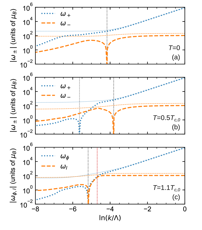
Examples of flowing and at zero-momentum are shown in Fig. 1. The figure considers a three-dimensional condensed gas at zero (a) and finite (b) temperature, and also a normal gas (c). The onset of polaron quasiparticles is manifested in the RG flow by the vanishing of . Note that two-dimensional gases show similar flows.
For values of lower than the physical polaron energy (thin lines), the flowing are always positive, signalling that at those large energies, no quasiparticle is formed. In contrast, for (thick lines), the flowing crosses zero during the RG flow at the points indicated by the vertical lines.
At zero temperature [panel (a)], only one quasiparticle branch crosses zero [57]. In contrast, at finite temperatures in the superfluid phase [panel (b)], both quasiparticle branches vanish during the RG flow. Therefore, the employed FRG ansatz predicts the formation of two quasiparticles at finite temperatures, similar to the results reported in Refs. [44, 45]. On the other hand, in the normal phase [panel (c)], both branches vanish at the same point, signalling only one quasiparticle branch, also consistent with previous studies [44]. Importantly, in the normal phase, both and vanish at the same scale, showing that the polaron-to-molecule crossover persists. In contrast, in the Fermi polaron problem, both branches vanish at different scales, signalling either a polaron or molecule phase [53].
Focusing again on the superfluid phase, the important question to answer is the origin of the two quasiparticle branches. As discussed in detail in Ref. [45], within their variational approach the multiple quasiparticles at finite temperatures are a result of the consideration of hole excitations. Indeed, such work found that even additional quasiparticles appear if more hole excitations are considered. Therefore, one would expect that the exact solution corresponds to a broad peak in the spectral function.
Within the employed FRG framework, the two quasiparticles are a result of the two pole branches [Eq. (9)]. These appear only due to the consideration of a two-channel model. Indeed, a one-channel model would only show one branch. Therefore, additional quasiparticles at finite temperatures would be manifested by either diverging three- and more-body couplings [66] or by considering additional auxiliary fields (such as trimer fields) which would produce additional poles [67, 68]. Such extensions will be considered in future work.
5 Polaron energy
To identify the physical polaron state, one needs to find the lower value of which produces a vanishing inverse impurity’s propagator at , which can be found self-consistently [53]. In this work, such state corresponds to a vanishing at [57]. Then, the found value of is identified as the ground-state polaron energy , which is reported in the following in the superfluid phase.
Note that within the gradient expansion employed in this work, only the energy of the lower quasiparticle branch can be well-identified. To obtain the full spectral function and find the energies of excited quasiparticles one needs to consider a frequency- and momentum-dependent ansatz, which is beyond the scope of the current work. For a detailed discussion see Ref. [53].
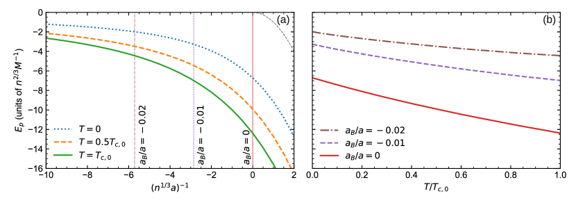
The polaron energy in a three-dimensional gas for the experimentally relevant gas parameter [17] is shown in Fig. 2. Panel (a) shows as a function of the inverse bath-impurity scattering length for selected temperatures, while panel (b) shows as a function of . The temperatures are scaled in terms of the critical temperature of the ideal Bose gas
| (13) |
Note that an interacting three-dimensional gas has a critical temperature slightly above that of an ideal gas (), which is correctly predicted by the FRG [61].
From both panels, it can be appreciated that the lowest quasiparticle energy decreases with increasing temperature, consistent with results from related works with analytical techniques [44, 45]. The same behaviour is found for other choices of gas parameters. However, the FRG calculations predict a much larger decrease of with the temperature than that reported with a variational approach (compare with Fig. 10 of Ref. [45]). Indeed, in this work the reported value of at almost double that at . As mentioned, while the FRG performs well at finite temperatures for one-component Bose gases [61], future work will need to consider a more sophisticated ansatz to quantify the accuracy of these results. In particular, three- or more-body correlations could have a more important role for . In addition, it is important to note that MC simulations have reported instead an increase of the polaron energy with the temperature [47].
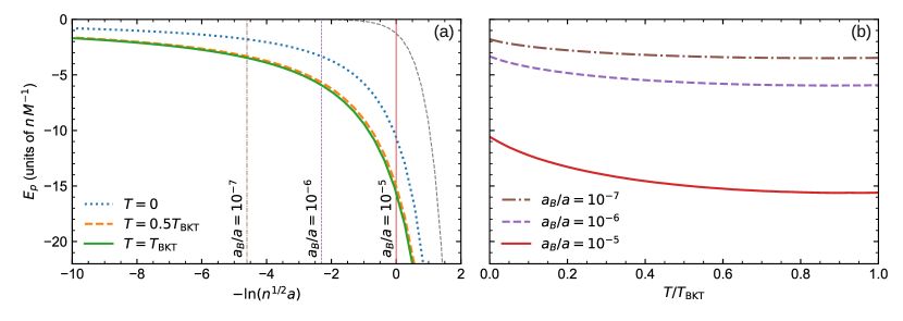
Polaron energies for a two-dimensional gas are then reported in Fig. 3. It considers a somewhat high gas parameter where three-body correlations are less relevant [57]. Note that the superfluid phase transition in two dimensions is driven by the Berezinskii-Kosterlitz-Thouless (BKT) mechanism [69, 70]. The BKT critical temperature is well-estimated by the FRG [62], and the critical exponents can be extracted from a pseudo-line of fixed point with good accuracy, even with a simple ansatz [71, 72]. However, the precise phase-transition temperature cannot be unambiguously located within a gradient expansion due to an incorrect slow vanishing of the flowing superfluid density . Therefore, here the temperatures are scaled in terms of the MC-predicted BKT critical temperature [73]
| (14) |
where , and is extracted from the FRG calculations.
As with the three-dimensional case, the polaron energy decreases with increasing temperature up to the phase transition. However, the two-dimensional polaron shows a distinct dependence on . Indeed, while decreases quickly at very low temperatures, converges for for any value of . This leads to almost indistinguishable results in panel (a) for and . As it can be appreciated in the figure, the value of at is roughly 50% larger than that at zero temperature. It has been checked that similar behaviours are found for other bath parameters.
6 Conclusions
This work has employed the FRG approach to study Bose polarons at finite temperatures in two and three dimensions across strong bath-impurity interactions. A simple ansatz with only two-body couplings was considered to test the FRG performance at finite temperatures. The emergence of two branches of quasiparticles in the superfluid phase at finite temperatures is found due to the consideration of a two-channel model. This is analogous to the onset of multiple quasiparticles also found with other techniques.
To improve the accuracy of the shown results, future work will need to consider a more sophisticated ansatz that includes additional effects. These include three- and more-body couplings, back-action of the impurity on the bath, and maybe the consideration of trimer fields to easily probe the onset of more quasiparticle branches. However, the most pressing extension is to consider momentum-dependent couplings to compute the full spectral function [53]. Such extension would provide access to excited states and extract other relevant properties, such as effective masses. Due to the complexity of this task, a self-consistent calculation of the propagators could be employed, as in Ref. [54] for Fermi polarons. A more in-depth examination of polaron properties around the BKT transition is also of interest, as recently studied in two-dimensional lattices [74]. Other related extensions include the use of the FRG for polarons in other scenarios, such as impurities immersed in a binary Bose gas [75, 76, 77] or across the BCS-BEC crossover [78, 79, 80, 81].
Acknowledgements.
This work was supported by ANID (Chile) through FONDECYT Postdoctorado No. 3230023.References
- [1] \NameLandau L. Pekar S. \REVIEWZh. Eksp. Teor. Fiz181948419.
-
[2]
\NameDagotto E. \REVIEWReviews of Modern Physics661994763.
https://link.aps.org/doi/10.1103/RevModPhys.66.763 -
[3]
\NameLee P. A., Nagaosa N. Wen X.-G. \REVIEWReviews of Modern Physics78200617.
https://link.aps.org/doi/10.1103/RevModPhys.78.17 -
[4]
\NameAlexandrov A. S., Samson J. H. Sica G. \REVIEWEPL (Europhysics Letters)100201217011.
https://iopscience.iop.org/article/10.1209/0295-5075/100/17011 -
[5]
\NameKutschera M. Wójcik W. \REVIEWPhysical Review C4719931077.
https://link.aps.org/doi/10.1103/PhysRevC.47.1077 -
[6]
\NameVidaña I. \REVIEWPhysical Review C1032021L052801.
https://link.aps.org/doi/10.1103/PhysRevC.103.L052801 -
[7]
\NameTajima H., Moriya H., Horiuchi W., Nakano E. Iida K. \BookIntersections of ultracold atomic polarons and nuclear clusters: How is a chart of nuclides modified in dilute neutron matter? arXiv:2310.19422 [astro-ph, physics:cond-mat, physics:nucl-th] (Oct. 2023).
http://arxiv.org/abs/2310.19422 -
[8]
\NameMassignan P., Zaccanti M. Bruun G. M. \REVIEWReports on Progress in Physics772014034401.
https://iopscience.iop.org/article/10.1088/0034-4885/77/3/034401 -
[9]
\NameChin C., Grimm R., Julienne P. Tiesinga E. \REVIEWReviews of Modern Physics8220101225.
https://link.aps.org/doi/10.1103/RevModPhys.82.1225 -
[10]
\NameParish M. M. Levinsen J. \BookFermi polarons and beyond arXiv:2306.01215 [cond-mat] (Jun. 2023).
http://arxiv.org/abs/2306.01215 -
[11]
\NameSchirotzek A., Wu C.-H., Sommer A. Zwierlein M. W. \REVIEWPhysical Review Letters1022009230402.
https://link.aps.org/doi/10.1103/PhysRevLett.102.230402 -
[12]
\NameKoschorreck M., Pertot D., Vogt E., Fröhlich B., Feld M. Köhl M. \REVIEWNature4852012619.
https://www.nature.com/articles/nature11151 -
[13]
\NameKohstall C., Zaccanti M., Jag M., Trenkwalder A., Massignan P., Bruun G. M., Schreck F. Grimm R. \REVIEWNature4852012615.
https://www.nature.com/articles/nature11065 -
[14]
\NameCetina M., Jag M., Lous R. S., Fritsche I., Walraven J. T. M., Grimm R., Levinsen J., Parish M. M., Schmidt R., Knap M. Demler E. \REVIEWScience354201696.
https://www.science.org/doi/10.1126/science.aaf5134 -
[15]
\NameScazza F., Valtolina G., Massignan P., Recati A., Amico A., Burchianti A., Fort C., Inguscio M., Zaccanti M. Roati G. \REVIEWPhysical Review Letters1182017083602.
https://link.aps.org/doi/10.1103/PhysRevLett.118.083602 -
[16]
\NameDarkwah Oppong N., Riegger L., Bettermann O., Höfer M., Levinsen J., Parish M., Bloch I. Fölling S. \REVIEWPhysical Review Letters1222019193604.
https://link.aps.org/doi/10.1103/PhysRevLett.122.193604 -
[17]
\NameJørgensen N. B., Wacker L., Skalmstang K. T., Parish M. M., Levinsen J., Christensen R. S., Bruun G. M. Arlt J. J. \REVIEWPhysical Review Letters1172016055302.
https://link.aps.org/doi/10.1103/PhysRevLett.117.055302 -
[18]
\NameHu M.-G., Van de Graaff M. J., Kedar D., Corson J. P., Cornell E. A. Jin D. S. \REVIEWPhysical Review Letters1172016055301.
https://link.aps.org/doi/10.1103/PhysRevLett.117.055301 -
[19]
\NameYan Z. Z., Ni Y., Robens C. Zwierlein M. W. \REVIEWScience3682020190.
https://www.sciencemag.org/lookup/doi/10.1126/science.aax5850 -
[20]
\NameSkou M. G., Skov T. G., Jørgensen N. B., Nielsen K. K., Camacho-Guardian A., Pohl T., Bruun G. M. Arlt J. J. \REVIEWNature Physics2021.
http://www.nature.com/articles/s41567-021-01184-5 -
[21]
\NamePeña Ardila L. A. P. Giorgini S. \REVIEWPhysical Review A942016063640.
https://link.aps.org/doi/10.1103/PhysRevA.94.063640 -
[22]
\NameGrusdt F., Schmidt R., Shchadilova Y. E. Demler E. \REVIEWPhysical Review A962017013607.
http://link.aps.org/doi/10.1103/PhysRevA.96.013607 -
[23]
\NameYoshida S. M., Endo S., Levinsen J. Parish M. M. \REVIEWPhysical Review X82018011024.
https://link.aps.org/doi/10.1103/PhysRevX.8.011024 -
[24]
\NameDrescher M., Salmhofer M. Enss T. \REVIEWPhysical Review A992019023601.
https://link.aps.org/doi/10.1103/PhysRevA.99.023601 -
[25]
\NameIchmoukhamedov T. Tempere J. \REVIEWPhysical Review A1002019043605.
https://link.aps.org/doi/10.1103/PhysRevA.100.043605 -
[26]
\NamePeña Ardila L. A., Jørgensen N. B., Pohl T., Giorgini S., Bruun G. M. Arlt J. J. \REVIEWPhysical Review A992019063607.
https://link.aps.org/doi/10.1103/PhysRevA.99.063607 -
[27]
\NameMassignan P., Yegovtsev N. Gurarie V. \REVIEWPhysical Review Letters1262021123403.
https://link.aps.org/doi/10.1103/PhysRevLett.126.123403 -
[28]
\NamePeña Ardila L. A. \REVIEWPhysical Review A1032021033323.
https://link.aps.org/doi/10.1103/PhysRevA.103.033323 -
[29]
\NameSchmidt R. Enss T. \REVIEWSciPost Physics132022054.
https://scipost.org/10.21468/SciPostPhys.13.3.054 -
[30]
\NameYegovtsev N., Massignan P. Gurarie V. \REVIEWPhysical Review A1062022033305.
https://link.aps.org/doi/10.1103/PhysRevA.106.033305 -
[31]
\NamePeña Ardila L. A. \REVIEWNature Reviews Physics42022214.
https://www.nature.com/articles/s42254-022-00443-5 -
[32]
\NameHryhorchak O., Panochko G. Pastukhov V. \REVIEWJournal of Physics B: Atomic, Molecular and Optical Physics532020205302.
https://iopscience.iop.org/article/10.1088/1361-6455/abb3ab -
[33]
\NamePeña Ardila L. A., Astrakharchik G. E. Giorgini S. \REVIEWPhysical Review Research22020023405.
https://link.aps.org/doi/10.1103/PhysRevResearch.2.023405 -
[34]
\NamePastukhov V. \REVIEWJournal of Physics B: Atomic, Molecular and Optical Physics512018155203.
https://iopscience.iop.org/article/10.1088/1361-6455/aacdcb -
[35]
\NameNakano Y., Parish M. M. Levinsen J. \REVIEWPhysical Review A1092024013325.
https://link.aps.org/doi/10.1103/PhysRevA.109.013325 -
[36]
\NameRath S. P. Schmidt R. \REVIEWPhysical Review A882013053632.
https://link.aps.org/doi/10.1103/PhysRevA.88.053632 -
[37]
\NameZinner N. T. \REVIEWEPL (Europhysics Letters)101201360009.
https://iopscience.iop.org/article/10.1209/0295-5075/101/60009 -
[38]
\NameLevinsen J., Parish M. M. Bruun G. M. \REVIEWPhysical Review Letters1152015125302.
https://link.aps.org/doi/10.1103/PhysRevLett.115.125302 -
[39]
\NameSun M., Zhai H. Cui X. \REVIEWPhysical Review Letters1192017013401.
http://link.aps.org/doi/10.1103/PhysRevLett.119.013401 -
[40]
\NameChristianen A., Cirac J. I. Schmidt R. \REVIEWPhysical Review A1052022053302.
https://link.aps.org/doi/10.1103/PhysRevA.105.053302 -
[41]
\NameBoudjemâa A. \REVIEWJournal of Physics A: Mathematical and Theoretical482015045002.
https://iopscience.iop.org/article/10.1088/1751-8113/48/4/045002 -
[42]
\NameLevinsen J., Parish M. M., Christensen R. S., Arlt J. J. Bruun G. M. \REVIEWPhysical Review A962017063622.
https://link.aps.org/doi/10.1103/PhysRevA.96.063622 -
[43]
\NamePastukhov V. \REVIEWJournal of Physics A: Mathematical and Theoretical512018195003.
https://iopscience.iop.org/article/10.1088/1751-8121/aab9c1/meta -
[44]
\NameGuenther N.-E., Massignan P., Lewenstein M. Bruun G. M. \REVIEWPhysical Review Letters1202018050405.
https://link.aps.org/doi/10.1103/PhysRevLett.120.050405 -
[45]
\NameField B., Levinsen J. Parish M. M. \REVIEWPhysical Review A1012020013623.
https://link.aps.org/doi/10.1103/PhysRevA.101.013623 -
[46]
\NameDzsotjan D., Schmidt R. Fleischhauer M. \REVIEWPhysical Review Letters1242020223401.
https://link.aps.org/doi/10.1103/PhysRevLett.124.223401 -
[47]
\NamePascual G. Boronat J. \REVIEWPhysical Review Letters1272021205301.
https://link.aps.org/doi/10.1103/PhysRevLett.127.205301 -
[48]
\NamePascual G., Wasak T., Negretti A., Astrakharchik G. E. Boronat J. \BookTemperature-induced miscibility of impurities in trapped Bose gases arXiv:2401.03926 [cond-mat] (Jan. 2024).
http://arxiv.org/abs/2401.03926 -
[49]
\NameWetterich C. \REVIEWPhysics Letters B301199390.
http://linkinghub.elsevier.com/retrieve/pii/037026939390726X -
[50]
\NameBerges J., Tetradis N. Wetterich C. \REVIEWPhysics Reports3632002223.
http://linkinghub.elsevier.com/retrieve/pii/S0370157301000989 -
[51]
\NameDupuis N., Canet L., Eichhorn A., Metzner W., Pawlowski J., Tissier M. Wschebor N. \REVIEWPhysics Reports91020211.
https://linkinghub.elsevier.com/retrieve/pii/S0370157321000156 -
[52]
\NameBoettcher I., Pawlowski J. M. Diehl S. \REVIEWNuclear Physics B - Proceedings Supplements228201263.
http://linkinghub.elsevier.com/retrieve/pii/S0920563212001612 -
[53]
\NameSchmidt R. Enss T. \REVIEWPhysical Review A832011063620.
https://link.aps.org/doi/10.1103/PhysRevA.83.063620 -
[54]
\NameKamikado K., Kanazawa T. Uchino S. \REVIEWPhysical Review A952017013612.
https://link.aps.org/doi/10.1103/PhysRevA.95.013612 -
[55]
\NameVon Milczewski J., Rose F. Schmidt R. \REVIEWPhysical Review A1052022013317.
https://link.aps.org/doi/10.1103/PhysRevA.105.013317 -
[56]
\Namevon Milczewski J. Schmidt R. \BookMomentum-dependent quasiparticle properties of the Fermi polaron from the functional renormalization group arXiv:2312.05318 [cond-mat] (Dec. 2023).
http://arxiv.org/abs/2312.05318 -
[57]
\NameIsaule F., Morera I., Massignan P. Juliá-Díaz B. \REVIEWPhysical Review A1042021023317.
https://link.aps.org/doi/10.1103/PhysRevA.104.023317 -
[58]
\NameIsaule F. Morera I. \REVIEWCondensed Matter720229.
https://www.mdpi.com/2410-3896/7/1/9 -
[59]
\NameMatsubara T. \REVIEWProgress of Theoretical Physics141955351.
https://academic.oup.com/ptp/article-lookup/doi/10.1143/PTP.14.351 -
[60]
\NameFloerchinger S. Wetterich C. \REVIEWPhysical Review A772008053603.
https://link.aps.org/doi/10.1103/PhysRevA.77.053603 -
[61]
\NameFloerchinger S. Wetterich C. \REVIEWPhysical Review A792009063602.
https://link.aps.org/doi/10.1103/PhysRevA.79.063602 -
[62]
\NameFloerchinger S. Wetterich C. \REVIEWPhysical Review A792009013601.
https://link.aps.org/doi/10.1103/PhysRevA.79.013601 -
[63]
\NameDiehl S. Wetterich C. \REVIEWNuclear Physics B7702007206.
https://linkinghub.elsevier.com/retrieve/pii/S0550321307001411 -
[64]
\NameLitim D. F. \REVIEWPhysics Letters B486200092.
https://linkinghub.elsevier.com/retrieve/pii/S0370269300007486 -
[65]
\NameMoroz S., Floerchinger S., Schmidt R. Wetterich C. \REVIEWPhysical Review A792009042705.
https://link.aps.org/doi/10.1103/PhysRevA.79.042705 -
[66]
\NameFloerchinger S., Moroz S. Schmidt R. \REVIEWFew-Body Systems512011153.
http://link.springer.com/10.1007/s00601-011-0231-z -
[67]
\NameSchmidt R., Rath S. Zwerger W. \REVIEWThe European Physical Journal B852012386.
http://link.springer.com/10.1140/epjb/e2012-30841-3 -
[68]
\NameJaramillo Ávila B. Birse M. C. \REVIEWPhysical Review A882013043613.
https://link.aps.org/doi/10.1103/PhysRevA.88.043613 - [69] \NameBerezinskii V. L. \REVIEWZh. Eksp. Teor. Fiz.591970907.
-
[70]
\NameKosterlitz J. M. Thouless D. J. \REVIEWJournal of Physics C619731181.
http://stacks.iop.org/0022-3719/6/i=7/a=010?key=crossref.f2d443370878b9288c142e398ad429b1 -
[71]
\NameGräter M. Wetterich C. \REVIEWPhysical Review Letters751995378.
https://link.aps.org/doi/10.1103/PhysRevLett.75.378 -
[72]
\NameGersdorff G. v. Wetterich C. \REVIEWPhysical Review B642001054513.
https://link.aps.org/doi/10.1103/PhysRevB.64.054513 -
[73]
\NamePilati S., Giorgini S. Prokof’ev N. \REVIEWPhysical Review Letters1002008140405.
https://link.aps.org/doi/10.1103/PhysRevLett.100.140405 -
[74]
\NameSantiago-García M. Camacho-Guardian A. \REVIEWNew Journal of Physics252023093032.
https://iopscience.iop.org/article/10.1088/1367-2630/acf72d -
[75]
\NameBighin G., Burchianti A., Minardi F. Macrì T. \REVIEWPhysical Review A1062022023301.
https://link.aps.org/doi/10.1103/PhysRevA.106.023301 -
[76]
\NameLiu N. Tu Z. C. \REVIEWJournal of Statistical Mechanics: Theory and Experiment20232023093101.
https://iopscience.iop.org/article/10.1088/1742-5468/acf8be -
[77]
\NameLiu N. \BookWeak and Strong Coupling Polarons in Binary Bose-Einstein Condensates arXiv:2401.11808 [cond-mat, physics:quant-ph] (Jan. 2024).
http://arxiv.org/abs/2401.11808 -
[78]
\NamePierce M., Leyronas X. Chevy F. \REVIEWPhysical Review Letters1232019080403.
https://link.aps.org/doi/10.1103/PhysRevLett.123.080403 -
[79]
\NameAlhyder R. Bruun G. M. \REVIEWPhysical Review A1052022063303.
https://link.aps.org/doi/10.1103/PhysRevA.105.063303 -
[80]
\NameHu H., Wang J., Zhou J. Liu X.-J. \REVIEWPhysical Review A1052022023317.
https://link.aps.org/doi/10.1103/PhysRevA.105.023317 -
[81]
\NameWang J., Liu X.-J. Hu H. \REVIEWPhysical Review A1052022043320.
https://link.aps.org/doi/10.1103/PhysRevA.105.043320