Black holes and gravitational waves from slow phase transitions

Abstract

Slow first-order phase transitions generate large inhomogeneities that can lead to the formation of primordial black holes (PBHs). We show that the gravitational wave (GW) spectrum then consists of a primary component sourced by bubble collisions and a secondary one induced by large perturbations. The latter gives the dominant peak if $\beta/H_{0}<10$, impacting, in particular, the interpretation of the recent PTA data. The GW signal associated with a particular PBH population is stronger than in typical scenarios because of a negative non-Gaussianity of the perturbations and it has a distinguishable shape with two peaks.

Introduction – In strongly supercooled phase transitions the Universe experiences a period of thermal inflation as the vacuum energy density of the false vacuum dominates over the radiation energy density before the transition occurs. If, in addition, the transition proceeds slowly there are large fluctuations in the duration of the thermal inflation in different patches. This leads to the formation of large inhomogeneities that source both primordial black holes (PBHs) and gravitational waves (GWs).

PBHs can form either during or after the transition. For the former case, the transition needs to be of first-order, proceeding by bubble nucleation, and PBHs form from subhorizon patches that are surrounded by the bubble walls Hawking et al. (1982); Kodama et al. (1982); Lewicki et al. (2023). In the latter case, the transition can be either a continuous transition where the field simply rolls to the true minimum Dimopoulos et al. (2019) or a first-order phase transitions Liu et al. (2022); Kawana et al. (2023); Gouttenoire and Volansky (2023) and PBHs form when the large fluctuations generated in the transition re-enter horizon.

This letter focuses on the formation of large inhomogeneities during a slow and strongly supercooled first-order phase transition. During such a process each Hubble patch includes only a handful of large bubbles and the perturbations originate from the fluctuations in the times of their nucleation. We compute the distribution of the perturbations using a new semi-analytic approach derived in the Supplemental Material and the PBH formation following the standard formalism (see Carr et al. (2021) for a review).

First-order phase transitions generate also a GW background Caprini et al. (2016, 2020). For strongly supercooled cases, it is sourced by the collisions of the bubble walls and relativistic fluid shells Kosowsky and Turner (1993); Lewicki and Vaskonen (2023). For slow transitions, there is also another source: the large perturbations. These GWs arise from the second-order terms in cosmological perturbation theory and their spectrum is widely studied in the literature (see Domènech (2021) for a review). In this letter, we show, for the first time, that the induced GW background is stronger than that from the bubble collisions if the transition is sufficiently slow. In particular, this is the case for transitions that lead to PBH formation. Our result has a large impact on the GW spectra in a significant part of the parameter spaces of quasi-conformal models capable of predicting such slow and strong transitions Jinno and Takimoto (2017); Iso et al. (2017); Marzola et al. (2017); Prokopec et al. (2019); Marzo et al. (2019); Baratella et al. (2019); Von Harling et al. (2020); Aoki and Kubo (2020); Delle Rose et al. (2020); Wang et al. (2020); Ellis et al. (2020); Baldes et al. (2021, 2022); Lewicki et al. (2021); Gouttenoire (2023).

The induced GW background is a signature also in the typical PBH formation scenarios, such as the constant-roll inflation Kannike et al. (2017); Germani and Prokopec (2017); Motohashi and Hu (2017); Karam et al. (2023). However, we find that the distribution of the perturbations generated in the first-order phase transition has a negative non-Gaussianity that suppresses the PBH formation. Consequently, the GW background associated with a certain abundance of PBHs, in this case, is stronger than e.g. in the case of constant-roll inflation where the non-Gaussianity is positive Tomberg (2023).

Formation of inhomogeneities – We consider an exponential bubble nucleation rate

$$\Gamma(t)=H_{0}^{4}e^{\beta t}\,,$$ (1)

where $H_{0}$ denotes the Hubble rate at $t=0$ and $\beta>0$ parametrizes the growth of the nucleation rate. The transition is slow if $\beta/H_{0}=\mathcal{O}(1)$ and the time it takes for the false vacuum fraction $\bar{F}(t)$ Guth and Weinberg (1983), averaged over a large volume, to get from $\bar{F}(t)\approx 1$ to $\bar{F}(t)\approx 0$ is comparable to the Hubble time $1/H_{0}$.

During the period of thermal inflation the comoving Hubble horizon radius $(aH)^{-1}$ shrinks and reaches its smallest value roughly at the percolation time $t_{p}$, defined as $\bar{F}(t_{p})=0.3$. The corresponding largest comoving wavenumber that exits horizon can be approximated as

$$k_{\rm max} =a(t_{p})H(t_{p})$$ (2)

$$\approx 1.6\times 10^{-7}{\rm Hz}\,\bigg{[}\frac{g_{*}}{100}\bigg{]}^{\frac{1}{2}}\bigg{[}\frac{100}{g_{*s}}\bigg{]}^{\frac{1}{3}}\frac{T_{\rm reh}}{\rm GeV}\,,$$

where $T_{\rm reh}\approx 8.5\times 10^{8}\,{\rm GeV}[g_{*}/100]^{-1/4}\sqrt{H_{0}/{\rm GeV}}$ is the temperature that the Universe reaches right after the thermal inflation and $g_{*}$ and $g_{*s}$ are the effective numbers of relativistic energy and entropy degrees of freedom at $T=T_{\rm reh}$.

The expanding bubbles convert the vacuum energy into kinetic and gradient energies of the bubble walls. The energy density in the walls scales in the same way as that of radiation Lewicki et al. (2023) and eventually decays to radiation after the bubble collisions. In total, the energy density in the bubble walls and radiation evolves as

$$\dot{\rho}_{r}+4H\rho_{r}=-\dot{\rho}_{v}\,,$$ (3)

where dot denotes the time derivative and $\rho_{v}$ is the vacuum energy density. Averaged over a large volume, the false vacuum energy density is given by $\bar{\rho}_{v}(t)=\bar{F}(t)\Delta V$, where $\Delta V$ denotes the vacuum energy density difference between the true and false vacua, and the Hubble rate by $H^{2}=8\pi G(\bar{\rho}_{r}+\bar{\rho}_{v})/3$, where $\bar{\rho}_{r}$ is the solution of Eq. (3) with $\rho_{v}(t)=\bar{\rho}_{v}(t)$. The evolution of the scale factor is determined by $\dot{a}=aH$.

On superhorizon scales each comoving Hubble patch evolves mutually independently and, in general, the false vacuum fraction evolves differently in different patches. We compute the false vacuum fraction $F_{k}(t)$ in different patches using the semi-analytical method derived in the Supplemental Material. This method accurately accounts for the fluctuations in the nucleation times and positions of the first $10$ bubbles and averages over the rest of the bubbles. For given values of $\beta/H_{0}$ and scale $k$, we generate $10^{4}$ realizations of the false vacuum fraction $F_{k}(t)$. Then, we solve the radiation energy density $\rho_{r,k}(t)$ from Eq. (3) with $\rho_{v}(t)=F_{k}(t)\Delta V$ and compute the density contrast as

$$\delta=\frac{\rho_{k}(t_{k})}{\bar{\rho}(t_{k})}-1\,,$$ (4)

where $\rho_{k}(t)=\rho_{r,k}(t)+F_{k}(t)\Delta V$ and $\bar{\rho}(t)=\bar{\rho}_{r}(t)+\bar{\rho}_{v}(t)$. We evaluate the density contrast at the time $t=t_{k}\geq t_{p}$ when the scale $k$ re-enters horizon, $a(t_{k})H(t_{k})=k$.

We show the probability distribution of $\delta$ in the upper panel of Fig. 1 at different $k$ values. The distributions are non-Gaussian with an exponential tail at negative $\delta$ and rapid fall at positive $\delta$. This follows from the distribution of the nucleation times of the bubbles that is given in the Supplemental Material. We find that the distribution can be fitted with

$$P_{k}(\delta)\propto\exp\left[\frac{\epsilon}{2}(\delta-\mu)-\frac{2}{\epsilon^{2}\sigma^{2}}\!\left(1-e^{\frac{\epsilon}{2}(\delta-\mu)}\right)^{\!2}\right],$$ (5)

where $\epsilon,\sigma>0$. The normalization factor is $\sqrt{2/\pi}[1+{\rm Erf}(\sqrt{2}{\epsilon\sigma})]^{-1}/\sigma$. In the lower panel of Fig. 1, we show the spectrum of $\delta$ as a function of $k$. We cut the spectrum at $k=k_{\rm max}$ as the smaller scales don’t exit horizon during the thermal inflation.

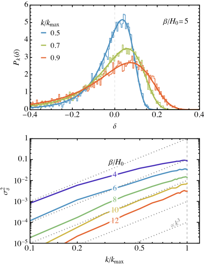
Figure 1: Upper panel: The probability distribution of the density contrast at different wavenumbers $k$. The histograms show the distributions of $10^{4}$ realizations and the solid curves the fits using Eq. (5). Lower panel: The variance of the density contrast as a function of $k$ for different values of $\beta/H_{0}$.

Primordial black holes – Large density perturbations lead to formation of PBHs as the radiation pressure is not enough to prevent the collapse of the overdense patch when it re-enters horizon Carr and Hawking (1974); Carr (1975). The masses of the PBHs follow the critical scaling law Choptuik (1993); Niemeyer and Jedamzik (1998, 1999)

$$M(\delta)=\kappa M_{k}(\delta-\delta_{c})^{\gamma}\,,$$ (6)

where $\delta$ is the density contrast and $M_{k}=M_{p}^{2}/(2H(t_{k}))=M_{0}H_{0}/H(t_{k})$ denotes the horizon mass when the scale $k$ re-enters horizon. The horizon mass during the inflation can be approximated as

$$M_{0}\approx 0.05M_{\odot}\left[\frac{100}{g_{*}}\right]^{\!\frac{1}{2}}\left[\frac{T_{\rm reh}}{\rm GeV}\right]^{-2}\,.$$ (7)

The parameters $\gamma$, $\kappa$ and $\delta_{c}$ depend on the profile of the overdensity and the equation of state of the Universe Musco (2019); Young et al. (2019); Musco et al. (2021); Franciolini et al. (2022); Musco et al. (2023). For simplicity, we use the fixed values $\gamma=0.36$, $\kappa=4$ and $\delta_{c}=0.5$. We note, however, that the equation of state of the Universe has not reached that of radiation when the smallest scales $k\simeq k_{\rm max}$ re-enter horizon.

The fraction of the total energy density that collapses to PBHs of mass $M$ is given by Carr (1975); Gow et al. (2021)

$$\beta_{k}(M) =\int_{\delta_{c}}{\rm d}\delta\frac{M}{M_{k}}P_{k}(\delta)\,\delta_{D}\!\left(\ln\frac{M}{M(\delta)}\right)$$ (8)

$$=\frac{\kappa}{\gamma}\left(\frac{M}{\kappa M_{k}}\right)^{\!1+\frac{1}{\gamma}}P_{k}(\delta(M))\,,$$

where $\delta_{D}$ denotes the Dirac delta function and $\delta(M)=\delta_{c}+[M/(\kappa M_{k})]^{1/\gamma}$. From $\beta_{k}(M)$ we obtain the present PBH mass function as

$$\psi(M)=\int\!{\rm d}\ln k\,\beta_{k}(M)\frac{\rho_{r}(T_{k})}{\rho_{c}}\frac{s(T_{0})}{s(T_{k})}$$ (9)

$$\approx 1.2\!\times\!10^{-9}\frac{g_{*}}{g_{*s}}\frac{T_{\rm reh}}{\rm GeV}\!\int\!{\rm d}\ln k\,\beta_{k}(M)\bigg{[}\frac{H(t_{k})}{H_{0}}\bigg{]}^{\frac{1}{2}},$$

where $\rho_{c}$ denotes the critical energy density of the Universe, $s(T)$ the entropy density, $T_{k}$ the temperature at the horizon re-entry of the scale $k$, $T_{0}$ the present CMB temperature and in the last step we approximated that $g_{*}$ and $g_{*s}$ don’t significantly change when the relevant scales re-enter horizon. The total PBH abundance is $\Omega_{\rm PBH}=\int{\rm d}\ln M\,\psi(M)$.

We compute the PBH mass function and abundance using the fits (5) of $P_{k}(\delta)$. By performing the computation for several values of $\beta/H_{0}$ and doing numerical fits, we find that the fraction of DM in PBHs, $f_{\rm PBH}\equiv\Omega_{\rm PBH}/\Omega_{\rm DM}$, is roughly of the form

$$f_{\rm PBH}=b_{1}\exp\!\left[-b_{2}e^{\beta/H_{0}}\right]\frac{g_{*}}{g_{*s}}\frac{T_{\rm reh}}{\rm GeV}$$ (10)

with $b_{1}\approx 2.8\times 10^{9}$ and $b_{2}\approx 0.246$, and the mass function is of form typical for the critical scaling law Vaskonen and Veermäe (2021),

$$\psi(M)\propto(M/M_{0})^{1+1/\gamma}\exp[-c_{1}(M/M_{0})^{c_{2}}]$$ (11)

with $c_{1}\approx 1.8$ and $c_{2}\approx 2.9$.

The abundance of PBHs is constrained by various observations: the effects of Hawking evaporation on big bang nucleosynthesis (BBN) and the extragalactic gamma-ray background Carr et al. (2010); Acharya and Khatri (2020), microlensing of stellar light Griest et al. (2014); Niikura et al. (2019a); Smyth et al. (2020); Tisserand et al. (2007); Niikura et al. (2019b); Allsman et al. (2001), lensing of supernovae Zumalacarregui and Seljak (2018), lensing of GW signals Urrutia and Vaskonen (2021); Urrutia et al. (2023), the binary merger rate Hütsi et al. (2021), survival of stars in dwarf galaxies Brandt (2016); Koushiappas and Loeb (2017), survival of wide binaries Monroy-Rodríguez and Allen (2014), Lyman-$\alpha$ forest Afshordi et al. (2003); Murgia et al. (2019) and limits on radiation emitted in accretion process Ricotti et al. (2008); Horowitz (2016); Ali-Haïmoud and Kamionkowski (2017); Poulin et al. (2017); Hektor et al. (2018); Hütsi et al. (2019); Serpico et al. (2020). In Fig. 2 we show the projection of the PBH constraints in the plane of the phase transition parameters calculated using the fits (10) and (11) and the method introduced in Carr et al. (2017). PBHs can constitute all DM in the asteroid mass window corresponding to $3\times 10^{4}\lesssim T_{\rm reh}/{\rm GeV}\lesssim 2\times 10^{7}$ and $\beta/H_{0}\approx 5$. The gray region on the left is excluded by the BBN/CMB constraint $T_{\rm reh}>5\,$MeV de Salas et al. (2015); Hasegawa et al. (2019); Allahverdi et al. (2020) and the region left from the blue dashed curve by the NANOGrav observations (see Fig. 4).

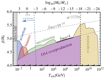
Figure 2: The PBH constraints projected to the plane of the phase transition parameters. The gray region is ecluded by the BBN/CMB constraint on the reheating temperature and the region left from the dashed blue curve by the PTA observations.

Compared to Liu et al. (2022); Kawana et al. (2023); Gouttenoire and Volansky (2023), our PBH computation includes three major improvements: 1) We account accurately for the distributions of the bubble nucleation times in the computation of the evolution of the false vacuum fraction while in Liu et al. (2022); Kawana et al. (2023); Gouttenoire and Volansky (2023) the fluctuations were only in the time when the nucleation begins. 2) We compute the perturbations as a function of $k\leq k_{\rm max}$ while in Liu et al. (2022); Kawana et al. (2023); Gouttenoire and Volansky (2023) only the scale of maximal $\delta$ was considered. 3) We include the critical scaling law in the computation of the PBH abundance computation. In total, these improvements result in a more realistic estimate of the PBH mass function and abundance. We emphasize, however, that our result (10) is based on fitting the distributions of $\delta$. This includes large uncertainties because the tail of the distribution relevant for PBH formation goes much beyond the range in which the distributions were obtained by generating $10^{4}$ realizations of the patches. This uncertainty affects only our PBH abundance estimates and not the secondary GWs discussed in the following for the first time.

Gravitational waves – For strongly supercooled phase transitions there are two distinct sources of GWs: the collisions of the bubble walls/relativistic fluid shells Kosowsky and Turner (1993); Huber and Konstandin (2008); Konstandin (2018); Cutting et al. (2018); Lewicki and Vaskonen (2020, 2021); Cutting et al. (2021); Lewicki and Vaskonen (2023) and the large curvature perturbations that induce production of GWs at second order Tomita (1975); Matarrese et al. (1994); Mollerach et al. (2004); Ananda et al. (2007); Baumann et al. (2007); Acquaviva et al. (2003); Domènech (2021).

The primary GW (PGW) spectrum from the collisions of the bubble walls/relativistic fluid shells is a broken power-law

$$\Omega_{\rm PGW}=\left[\frac{\beta}{H}\right]^{-2}\!\!\frac{A(a+b)^{c}S_{H}(k,k_{\rm max})}{\left[b\left({k}/{k_{p}}\right)^{\!-\frac{a}{c}}+a\left({k}/{k_{p}}\right)^{\!\frac{b}{c}}\right]^{\!c}}\,,$$ (12)

where $k_{p}\approx 0.7k_{\rm max}\beta/H_{0}$ and $A=5.1\times 10^{-2}$ are the peak wavenumber and amplitude of the spectrum, $a=b=2.4$, $c=4$ Lewicki and Vaskonen (2023) and

$$S_{H}(k,k_{\rm max})=\left[1+\frac{\Omega_{\rm CT}(k_{\rm max})}{\Omega_{\rm CT}(k)}\left(\frac{k}{k_{\rm max}}\right)^{\!a}\right]^{-1}\,.$$ (13)

The function $\Omega_{\rm CT}(k)$ accounts for the causality-limited tail of the spectrum at $k\lesssim k_{\rm max}$, where $k_{\rm max}$ is given by (2). In pure radiation dominance $\Omega_{\rm CT}(k)\propto k^{3}$ Caprini et al. (2009) but becomes slightly less steep e.g. around the QCD transition Franciolini et al. (2023a). We note the results we use for the primary GW spectrum are obtained from simulations neglecting the expansion of the Universe. Including it may lead to an additional suppression of the primary spectrum Zhong et al. (2021).

The spectrum of the secondary GWs (SGWs) reads Kohri and Terada (2018); Espinosa et al. (2018); Inomata and Terada (2020)

$$\Omega_{\rm SGW}\approx\frac{1}{3}\int_{1}^{\infty}\!\!{\rm d}t \int_{0}^{1}\!{\rm d}s\,\mathcal{I}_{t,s}^{2}\left[\frac{(t^{2}-1)(1-s^{2})}{t^{2}-s^{2}}\right]^{2}$$ (14)

$$\times\mathcal{P}_{\zeta}\left(k\frac{t-s}{2}\right)\mathcal{P}_{\zeta}\left(k\frac{t+s}{2}\right),$$

where $\mathcal{P}_{\zeta}$ denotes the curvature power spectrum and $\mathcal{I}_{t,s}$ the transfer function,

$${\cal I}_{t,s}^{2} =\!\frac{288(s^{2}+t^{2}-6)^{2}}{(t^{2}-s^{2})^{6}}\!\Bigg{[}\!\frac{\pi^{2}}{4}(s^{2}+t^{2}-6)^{2}\theta(t^{2}-3)$$ (15)

$$+\left(t^{2}-s^{2}-\frac{1}{2}(s^{2}+t^{2}-6)\ln\left|\frac{t^{2}-3}{3-s^{2}}\right|\right)^{2}\Bigg{]}.$$

We neglect the corrections arising from the non-Gaussian shape of the perturbations as the abundance of the induced GWs is mainly determined by the characteristic amplitude of perturbations. This slightly underestimates the SGW abundance Unal (2019); Cai et al. (2019); Yuan and Huang (2021); Adshead et al. (2021); Abe et al. (2023); Ellis et al. (2024). We use the linear relation between the density contrast and the curvature perturbation at the time of horizon crossing, $\zeta=9\delta/4$, to compute $\mathcal{P}_{\zeta}$ from the spectrum of $\delta$ shown in the lower panel of Fig. 1.

In Fig. 3 we show the total present abundance of the GWs produced in the phase transition,

$$\Omega_{\rm GW}h^{2}\approx 1.6\times 10^{-5}\!\left[\frac{g_{*}}{100}\right]\!\left[\frac{g_{*s}}{100}\right]^{\!-\frac{4}{3}}\left[\Omega_{\rm PGW}+\Omega_{\rm SGW}\right],$$ (16)

for different values of $\beta/H_{0}$. The spectrum has two peaks corresponding to the two sources. The SGW spectrum exhibits a low-frequency tail that scales roughly as $\propto k^{2.5}$, a narrow peak at $k\simeq k_{\rm max}$ and a sharp fall-off at $k>k_{\rm max}$. The peak amplitude of the secondary spectrum can be approximated by

$$\Omega_{\rm SGW}h^{2}|_{\rm peak}\approx 10^{-4}\!\left[\frac{g_{*}}{100}\right]\!\left[\frac{g_{*s}}{100}\right]^{\!-\frac{4}{3}}e^{-\beta/H_{0}}\,,$$ (17)

while its shape does not change very significantly with $\beta/H_{0}$. The PGW spectrum dominates at $k>k_{\rm max}$ and has its maximum at $k_{p}>k_{\rm max}$. As the peak amplitude of the PGW spectrum scales only as a power-law, $\Omega_{\rm PGW}\propto(\beta/H_{0})^{-2}$, it becomes dominant at large $\beta/H_{0}$ values. We find that the peak amplitudes of the primary and secondary GW spectra are the same for $\beta/H_{0}\approx 10$.

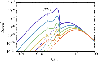
Figure 3: The solid curves show the sum of the primary and secondary GW spectra from a phase transition as a function of the wavenumber $k=2\pi f$. The dashed curves show the primary spectrum alone. The vertical dashed line shows the inverse Hubble radius at the end of the transition, $k_{\rm max}$. For smaller wavenumbers, the secondary spectrum is the dominant contribution while the standard primary spectrum dictates the shape at scales that were inside the horizon at the time of the transition.

Recently, the pulsar timing array collaborations have reported strong evidence for a stochastic GW background at nHz frequencies Agazie et al. (2023a, b); Antoniadis et al. (2023a, b, c); Reardon et al. (2023a); Zic et al. (2023); Reardon et al. (2023b); Xu et al. (2023); Afzal et al. (2023); Agazie et al. (2023c). The primary spectrum from a strong phase transition was already featured in a multi-model analysis comparing how well different astrophysical and cosmological models fit this signal Ellis et al. (2024). In Fig. 4 we show an improved fit including both the primary and secondary spectra. It is clear that the inclusion of the secondary spectrum is crucial and the improved reconstructed parameter space is not compatible with the previous results. In particular, the best-fit point moves to significantly higher temperatures, $T_{\rm reh}=2.7\,$GeV with $\beta/H_{0}=7.3$. However, the quality of the fit changes very marginally by $\Delta\chi^{2}\approx 0.06$ and the model comparison in Ellis et al. (2024) remains valid. The negative non-Gaussianity of the perturbations is important here, as in models with positive or zero non-Gaussianity the second-order GWs are disfavoured by the PTA fit due to the PBH overproduction Franciolini et al. (2023b).

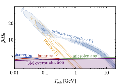
Figure 4: The blue contours show the fit of the spectrum including the primary and secondary contributions to the recent NANOGrav data. The orange contours show, for comparison, the same fit using only the primary spectrum. The coloured regions at the bottom are excluded by constraints on the PBHs produced in the transition.

In Fig. 5 we show the regions of the phase transition parameters that planned GW experiments will be able to probe with signal-to-noise ratio ${\rm SNR}\geq 10$. Solid lines show where the sum of the primary and secondary phase transition spectra will be probed while the dashed ones indicate only regions where the secondary spectrum dominates and will be detectable. We include the reach of LISA Bartolo et al. (2016); Caprini et al. (2019); Auclair et al. (2023), AEDGE El-Neaj et al. (2020); Badurina et al. (2021), AION Badurina et al. (2020, 2021), The Einstein Telescope (ET) Punturo et al. (2010); Hild et al. (2011), the Nancy Roman telescope Wang et al. (2022), and LVK through the design sensitivity of LIGO Aasi et al. (2015); Abbott et al. (2016, 2019). The region below the red line is excluded by the BBN/CMB constraint on the total abundance of GWs, $\Omega_{\rm GW}h^{2}\lesssim 1.8\times 10^{-6}$ Kohri and Terada (2018); Pagano et al. (2016) and the dark brown dot-dashed line is the constraint from the current LVK (O3) data Abbott et al. (2021). The gray region shows where the produced population of PBHs is constrained (see. Fig. 2 for details). While the previously known primary spectra dominate for faster transitions with large $\beta/H_{0}$ there is a large part of parameter space where the secondary spectra will also be detectable. This primarily includes slow transitions with $\beta/H_{0}\lesssim 40$. The region where the secondary GWs would be observable also extends to transitions with relatively high reheating temperatures and peak frequencies as there we mostly observe the low-frequency tail which falls off slower for the secondary contribution than for the primary one. Remarkably, the current LVK constraint reaches above the PBH constraints. This is mainly because of the secondary GW component and the suppression of the PBH formation arising from the negative non-Gaussianity.

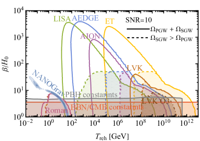
Figure 5: The solid curves show the parts of the parameter space within reach of indicated experiments with ${\rm SNR}=10$. The dashed curves indicate the parts where ${\rm SNR}=10$ is reached by integrating only over the frequency range where the secondary spectrum dominates. The gray region is excluded by the PBH constraints shown in Fig. 2 and the red region by CMB and BBN constraints on the GW abundance. The blue area corresponds to the fit to NANOGrav data from Fig. 4.

Conclusions – In this letter we have studied the large inhomogeneities generated in slow and strongly supercooled first-order phase transitions. We have derived a new contribution to the GW spectrum, the secondary GWs, resulting from the phase transition. The process behind this contribution is identical to the well-known scalar-induced GWs associated with primordial inflation. We have shown that the secondary GWs dominate the spectrum and have a very significant impact on its shape close to the peak provided the transition is slow enough. This will have a large impact on the resulting spectra in a significant part of parameter spaces in scale-invariant models capable of predicting such slow and strong transitions.

We have computed also the distribution of the perturbations finding it to have a negative non-Gaussianity. This has allowed us to better estimate the formation of PBHs in phase transitions. We have provided a simple fit to the abundance and mass function of the resulting PBH population. We have shown that models with a phase transition occurring at $T_{\rm reh}\approx 10^{6}\,$GeV with $\beta/H_{0}\approx 5$ would provide the entirety of the observed dark matter in the form of asteroid mass PBHs and produce a strong GW spectrum within the reach of LISA, ET, AION and AEDGE, however, inaccessible to LVK. The smoking gun signature of our scenario is the peculiar shape of GW spectum, including two peaks corresponding to the horizon scale at the end of the transition and the characteristic size of the bubbles.

Computation of the false vacuum fraction – The average false vacuum fraction is given by the probability that the given point still is in the false vacuum at time $t$:

$$\bar{F}(t)=\exp\left[-\frac{4\pi}{3}\int_{-\infty}^{t}\!{\rm d}t_{n}\,\Gamma(t_{n})a(t_{n})^{3}R(t,t_{n})^{3}\right]\,.$$ (S1)

Here $R(t_{n},t)$ is the comoving radius of a bubble nucleated at time $t_{n}$. The bubble radius increases linearly with the conformal time. In a finite volume, the evolution of the false vacuum fraction can deviate significantly from $\bar{F}(t)$. In the following, we derive a semi-analytical way of computing the false vacuum fraction in a finite comoving volume.

Consider a spherical comoving volume $V(k)=4\pi k^{-3}/3$. We divide the false vacuum fraction $F_{k}(t)$ in the volume $V(k)$ into two pieces: the contribution from the first $j_{c}$ bubbles and the contribution from the rest of the bubbles,

$$F_{k}(t)=F_{k}^{(j\leq j_{c})}(t)F_{k}^{(j>j_{c})}(t)\,.$$ (S2)

As the bubble nucleation is a Poisson process, the probability distribution of the time when the $j$th bubble reaches or nucleates within that volume is given by

$$p_{t,j}(t;k)=\frac{{\rm d}\bar{N}_{k}(t)}{{\rm d}t}\frac{\bar{N}_{k}(t)^{j-1}}{\Gamma(j)}e^{-\bar{N}_{k}(t)}\,,$$ (S3)

where

$$\bar{N}_{k}(t)=\frac{4\pi}{3}\int_{-\infty}^{t}{\rm d}t_{n}\,\Gamma(t_{n})a(t_{n})^{3}\left[k^{-1}+R(t;t_{n})\right]^{3}$$ (S4)

is the expected number of bubbles that nucleate inside or reach the volume $a^{3}V(k)$ by the time $t$. We show the distributions $p_{t,j}$ in Fig S1 for $j=1,2,4,8$, $k=k_{\rm max}/3$ and $\beta/H_{0}=5$.

The bubble that at time $t$ reaches or nucleates inside the volume $V(k)$ must have nucleated within the distance $d<k^{-1}+R(t;t_{n})$ where $t_{n}$ is its nucleation time. The probability distribution of $d$ increases as $d^{2}$ up to that maximal radius:

$$p_{d}(d;t,k)=\frac{-3d^{2}}{1-\bar{F}(t)}\!\int_{-\infty}^{t}\!\!{\rm d}t_{n}\dot{\bar{F}}(t_{n})\frac{\theta(k^{-1}+R(t;t_{n})-d)}{\left[k^{-1}+R(t;t_{n})\right]^{3}}.$$ (S5)

The volume of the intersection of spheres of radius $R$ and $r$ whose centres are separated by distance $d$ is

$$V_{\rm int}(d,R,r)\!=\!\begin{cases}\frac{4\pi}{3}d^{3}\xi(\frac{R}{d},\frac{r}{d})&|R-r|\leq d\leq R+r\\ \frac{4\pi}{3}\min[r,R]^{3}&d<|R-r|\\ 0&d>R+r\end{cases},$$ (S6)

where $\xi(x,y)=(1-x-y)^{2}(1+2(x+y)-3(x-y)^{2})/16$. So, the $j$th bubble covers the fraction

$$f(t;t_{j},d_{j},k)\equiv\frac{V_{\rm int}(d_{j},\max[0,d_{j}-k^{-1}]+R(t;t_{j}),k^{-1})}{V(k)}$$ (S7)

of the volume $V(k)$.

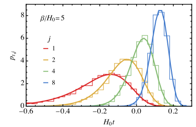
Figure S1: The probability distributions of the nucleation times of the 1st, 2nd, 4th and 8th bubbles inside the volume $V(k_{\rm max}/3)$. The histograms result from $10^{3}$ numerical simulations and the smooth curves show the function (S3).

The contribution from the first $j_{c}$ bubbles can be computed either by numerical simulations where these bubbles are nucleated inside some volume according to the nucleation rate $\Gamma(t)$ or semi-analytically by picking random numbers from the distributions $p_{t,j}$ and $p_{d}$. The function $F_{k}^{(j<j_{c})}$ can be simply integrated from the numerical simulations whereas in the semi-analytical approach, it can be approximated as

$$F_{k}^{(j\leq j_{c})}(t)\approx\exp\!\bigg{[}-\sum_{j=1}^{j_{c}}f(t;t_{j},d_{j},k)\bigg{]}\,.$$ (S8)

For the main results of the paper, we use the semi-analytical approach which is computationally less expensive allowing large scans of the parameters including the wavenumber $k$ and the inverse time scale of the transition $\beta$. We have, however, performed cross-checks of the results with numerical simulations and found a very good agreement between the approaches. In particular, as shown in Fig. S1, the probability distribution of the bubble nucleation times (S3), matches with the results of numerical simulations.

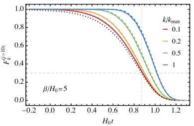
Figure S2: The contribution to the false vacuum fraction from the bubbles nucleating after the first $j_{c}=10$ bubbles computed using Eqs. (S9) and (LABEL:eq:FJ). For the solid curves $J=100$ and for the dashed curves $J=j_{c}+1=11$. The dotted black curve shows $\bar{F}(t)$.

The contribution from the rest of the bubbles can be approximated as

$$F_{k}^{(j>j_{c})}(t)\approx\exp\!\bigg{[}- \!\!\!\!\sum_{j=j_{c}+1}^{\infty}\int{\rm d}t_{j}{\rm d}d_{j}\,p_{t,j}(t_{j};k)$$ (S9)

$$\times p_{d}(d_{j};t_{j},k)f(t;t_{j},d_{j},k)\bigg{]}.$$

We can further split the sum in (S9) in two parts at $j=J\gg 1$ so that at $j\geq J$ the distribution (S3) can be approximated by the delta function

$$p_{t,j}(t;k)=\frac{{\rm d}\bar{N}_{k}(t)}{{\rm d}t}\delta(\bar{N}_{k}(t)-j)$$ (S10)

and the sum over $j$ by an integral. Then, the $j\geq J$ part is just a simple two-dimensional numerical integral:

$$\sum_{j=J}^{\infty}\int{\rm d}t_{j}{\rm d}d_{j}\,p_{t,j}(t_{j};k)p_{d}(d_{j};t_{j},k)f(t;t_{j},d_{j},k)$$ (S11)

$$\approx\int\!{\rm d}t^{\prime}{\rm d}d^{\prime}\,\theta\!\left(\bar{N}_{k}(t^{\prime})-J\right)\!\frac{{\rm d}\bar{N}_{k}(t^{\prime})}{{\rm d}t^{\prime}}p_{d}(d^{\prime};t^{\prime},k)f(t;t^{\prime},d^{\prime},k).$$

We show the function $F_{k}^{(j>j_{c})}(t)$ in Fig. S2   for $j_{c}=10$ and two different choices of $J$: $J=100$ and $J=j_{c}+1=11$. We see that the choice of $J$ does not have a large effect and already $J=j_{c}+1$ works very well. For our main results, we use $J=100$.

From Fig. S2 we see also that, as expected, the function $F_{k}^{(j>j_{c})}(t)$ approaches the expected evolution $\bar{F}(t)$ at small $k$. This can be shown analytically: Taking a large enough volume ($k^{-1}$ much larger than the average bubble radius), the bubbles nucleating outside the volume can be neglected. In this limit, we can use the approximations

$$\bar{N}_{k}(t)\approx\frac{4\pi}{3}k^{-3}\int_{-\infty}^{t}{\rm d}t_{n}\,\Gamma(t_{n})a(t_{n})^{3}\,,$$ (S12)

and

$$f(t;t_{j},d_{j},k)\approx(kR(t;t_{j}))^{3}\,,$$ (S13)

which give

$$F_{k}^{(j>j_{c})}(t)\approx\exp\!\bigg{[}\!-\!\!\!\sum_{j=j_{c}+1}^{J-1}\int{\rm d}t_{j}\,p_{t,j}(t_{j};k)(kR(t;t_{j}))^{3}$$ (S14)

$$\quad-\frac{4\pi}{3}\int\!{\rm d}t^{\prime}\theta\!\left(\bar{N}_{k}(t^{\prime})-J\right)\Gamma(t^{\prime})a(t^{\prime})^{3}R(t;t^{\prime})^{3}\bigg{]}.$$

The $J\to 0$ limit or, equivalently, the $k\to 0$ limit, as in that case the first few bubbles can be neglected, matches the average evolution (S1), $\lim_{J\to 0}F_{k}(t)=\lim_{k\to 0}F_{k}(t)=\bar{F}(t)$.

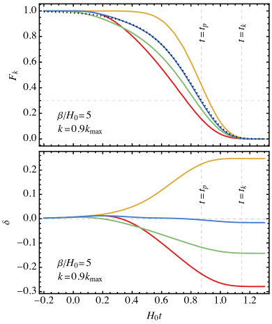
Figure S3: Upper panel: The colourful curves represent the false vacuum fraction in four patches of radius $1/(0.9k_{\rm max})$ and the dotted curve shows the time evolution of the expected false vacuum fraction $\bar{F}(t)$. Lower panel: The evolution of the density contrast in the same four patches as shown in the upper panel. The vertical dashed lines indicate the percolation time $t_{p}$ and the time $t_{k}$ when the scales associated with these patches re-enter the horizon.

Computation of the density contrast – We show the evolution of the false vacuum fraction in four patches corresponding to the wavenumber $k=0.9k_{\rm max}$ in the upper panel of Fig. S3. These are computed with $j_{c}=10$ and $J=100$. From $F_{k}(t)$ we can compute the density contrast

$$\delta(t)=\frac{\rho_{k}(t)}{\bar{\rho}(t)}-1\,,$$ (S15)

by solving the total energy density from the continuity equation describing the production of radiation from the decaying false vacuum in an expanding universe. We show the density contrast as a function of time in the lower panel of Fig. S3 for the same patches as in the upper panel.

In the main text, we use the distribution of $\delta$ at the horizon re-entry, $t=t_{k}$, to estimate the PBH and GW abundances generated in the phase transition. Here, we investigate how the distribution of $\delta$ depends on the choice of $j_{c}$. We generate $10^{4}$ realizations of $F_{k}^{j\leq j_{c}}(t)$ for $k=0.9k_{\rm max}$, $\beta/H_{0}=5$ and different choices of the cut-off: $j_{c}=1,2,5,10$. For each resulting $F_{k}(t)$ we compute $\delta(t)$ and evaluate them at the percolation temperature $t_{p}$ to obtain the distribution of $\delta(t_{p})$ that we denote by $P_{k}(\delta)$. As shown in Fig. S4, too small choices of $j_{c}$ underestimate the width of the distribution but already from $j_{c}=5$ to $j_{c}=10$ the distribution remains almost unchanged. For our main results, we use $j_{c}=10$.

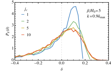
Figure S4: The probability distribution of the density contrast for different choices of the cut-off $j_{c}$.