Controller synthesis for input-state data
with measurement errors

Abstract

We consider the problem of designing a state-feedback controller for a linear system, based only on noisy input-state data. We focus on input-state data corrupted by additive measurement errors, which, albeit less investigated, are as relevant as process disturbances in applications. For energy and instantaneous bounds on these measurement errors, we derive linear matrix inequalities for controller design where the one for the energy bound is actually equivalent to robust stabilization of all systems consistent with the noisy data points.

I Introduction

We would like to design a state feedback controller for a discrete-time linear time-invariant (LTI) system without knowing the parameter matrices $(A,B)$ of its state equation, but with only input-state measurements. When such measurements are noise-free and enjoy persistence of excitation, they identify the parameter matrices exactly. The interesting scenario is thus for noisy measurements. In practical settings, it is reasonable and desirable that the noise in the measurements is bounded in some sense. The combination of the data generation mechanism and the noise bound yields a set of parameter matrices consistent with data, as in set membership identification [1]. Since the actual system is indistinguishable from all others in the set, our goal is to asymptotically stabilize all systems consistent with data. We share this approach with many recent works on (direct) data driven control [2, 3, 4, 5, 6].

Within this framework, however, the noise can enter the system in different ways when data are generated and different bounds on the noise can be postulated. As for the first aspect, a large part of the recent literature on data-driven control has considered a process disturbance, which captures unmodeled dynamics in the state equation. Still, less attention has been devoted to additive disturbances corrupting the input, which capture actuator inaccuracies, or corrupting the state, which capture sensor inaccuracies. These additive disturbances correspond to the setting known as errors-in-variables in classical system identification [7, 8, 9], and we term them here measurement errors. Measurement errors are commonly postulated to have an energy bound or an instantaneous bound [10, §I]: the former considers the whole sequence of the errors acting during data collection, see (12) below, whereas the latter considers each of such error instances, see (14) below. The treatment of instantaneous bounds is relevant for analogous advantages to those evidenced in [11] for process disturbances.

Based on this discussion, the case of measurement errors with instantaneous bounds is particularly relevant for applications, since such norm bounds on input or state errors can be inferred based on the actuator or sensor characteristics point-wise in time, in a relatively easier way than, e.g., energy bounds on process disturbances. We provide linear matrix inequalities (LMIs) to design a state-feedback controller for the setting of measurement errors with both energy and instantaneous bounds.

Related literature. In [11] and [12], data is generated by an LTI system affected by a process disturbance. Here, we depart from that setting and consider instead input-state data affected by measurement errors, in an error-in-variables setting. In [2], sufficient conditions for controller design are given when the measurement error on the state satisfies an energy bound, whereas we provide necessary and sufficient conditions here. Measurement errors and a process disturbance, which satisfy an instantaneous bound (in $\infty$-norm), are considered in [13]. To handle bilinearity in the set of system parameters, [13] formulates the controller design as a polynomial optimization problem, which is approximated by a converging sequence of sum-of-squares programs. Here, an instrumental result, Proposition 1, enables the controller design by solving a single LMI. Finally, the results in this paper complement those in [14]. While [14] addresses the case of output feedback, with input and output data corrupted by measurement errors, we consider here state feedback. Focusing on the special case of state feedback, we give stronger conditions than those in [14], namely a necessary and sufficient condition in Theorem 1 instead of the sufficient conditions in [14, Thm. 1]. Besides, [14] treats only energy bounds whereas we treat also instantaneous ones here.

Contribution. For measurement errors with energy and instantaneous bounds, we obtain two corresponding LMIs in Theorems 1 and 2. These LMIs depend only on the collected data and the postulated bounds, and enable the design of a state-feedback controller. Such controller is guaranteed to asymptotically stabilize all systems consistent with data, and the actual one in particular. Importantly, Theorem 1 takes the form of a necessary and sufficient condition. We also provide the independently relevant Proposition 1, which can be interpreted as a matrix elimination result.

II Preliminaries

II-A Notation

The identity matrix of size $n$ and the zero matrix of size $m\times n$ are $I_{n}$ and $0_{m\times n}$: the indices are dropped when no confusion arises. The largest eigenvalue of a symmetric matrix $M$ is $\lambda_{\max}(M)$. The largest and smallest singular values of a matrix $M$ are $\sigma_{\max}(M)$ and $\sigma_{\min}(M)$. The 2-norm of a vector $v$ is $|v|$. The induced 2-norm of a matrix $M$ is $\|M\|$ and is equivalent to $\sigma_{\max}(M)$. For matrices $M$, $N$ and $O$ of compatible dimensions, we abbreviate $MNO(MN)^{\top}$ to $MN\cdot O[\star]^{\top}$, where the dot in the second expression clarifies unambiguously that $MN$ is the term to be transposed. For a symmetric matrix $\left[\begin{smallmatrix}M&N\\ N^{\top}&O\end{smallmatrix}\right]$, we may use the shorthand writing $\left[\begin{smallmatrix}M&N\\ \star&O\end{smallmatrix}\right]$. For a positive semidefinite matrix $M$, $M^{1/2}$ is its unique positive semidefinite square root [15, p. 440].

II-B Matrix elimination result

The next result is key for the sequel.

Proposition 1.

Consider matrices $E\in\mathbb{R}^{n_{1}\times n_{2}}$, $F\in\mathbb{R}^{n_{1}\times n_{3}}$, $G\in\mathbb{R}^{n_{3}\times n_{3}}$ with $G=G^{\top}\succeq 0$. Then,

$$EE^{\top}\preceq FGF^{\top}$$ (1a)

if and only if there exists $$D\in\mathbb{R}^{n_{3}\times n_{2}}$$ such that

$$E=FD,\quad DD^{\top}\preceq G.$$ (1b)

Proof.

($\Longleftarrow$) Trivial.
($\Longrightarrow$) We need to show that if (1a) holds, then there exists $D$ such that (1b) holds. If $G=0$, it must be $E=0$ and $D=0$ yields (1b). We then consider $G\neq 0$ in the rest of the proof. For $G\neq 0$, there exist a real orthogonal matrix $U$ (i.e., $UU^{\top}=U^{\top}U=I$) and a diagonal positive definite $\Lambda_{1}$ such that an eigendecomposition of $G$ is

$$G=U\left[\begin{smallmatrix}\Lambda_{1}&0\\ 0&0\end{smallmatrix}\right]U^{\top}=\begin{bmatrix}U_{1}~{}U_{2}\end{bmatrix}\left[\begin{smallmatrix}\Lambda_{1}&0\\ 0&0\end{smallmatrix}\right]\begin{bmatrix}U_{1}^{\top}\\ U_{2}^{\top}\end{bmatrix}=U_{1}\Lambda_{1}U_{1}^{\top},$$

which becomes $G=U\Lambda_{1}U^{\top}$ in case $G\succ 0$. By the eigendecomposition of $G$, (1a) is equivalent to

$$EE^{\top}\preceq FU_{1}\Lambda_{1}U_{1}^{\top}F^{\top}.$$ (2)

If there exists $D_{1}$ such that

$$E=FU_{1}D_{1}\text{ and }D_{1}D_{1}^{\top}\preceq\Lambda_{1},$$ (3)

then there exists $D=U_{1}D_{1}$ such that $E=FD$ and $DD^{\top}=U_{1}D_{1}D_{1}^{\top}U_{1}^{\top}\preceq U_{1}\Lambda_{1}U_{1}^{\top}=G$, by the eigendecomposition of $G$, and this would show (1b). Then, the rest of the proof focuses on finding $D_{1}$ such that (3) holds. If $FU_{1}=0$, it must be from (2) that $E=0$, and any $D_{1}$ with $D_{1}D_{1}^{\top}\preceq\Lambda_{1}$ satisfies (3). If $FU_{1}\neq 0$, there always exists a nonsingular matrix $V$ such that $VFU_{1}=\left[\begin{smallmatrix}F_{1}\\ 0\end{smallmatrix}\right]$ with $F_{1}$ full row rank, which can be obtained as the reduced row echelon form [15, p. 11-12]. Let $VE=:\left[\begin{smallmatrix}E_{1}\\ E_{2}\end{smallmatrix}\right]$ where $E_{1}$ has as many rows as $F_{1}$. In this case, (2) implies

$$VEE^{\top}V^{\top}\preceq VFU_{1}\Lambda_{1}U_{1}^{\top}F^{\top}V^{\top}$$

$$\iff\left[\begin{smallmatrix}E_{1}\\ E_{2}\end{smallmatrix}\right]\left[\begin{smallmatrix}E_{1}\\ E_{2}\end{smallmatrix}\right]^{\top}\preceq\left[\begin{smallmatrix}F_{1}\\ 0\end{smallmatrix}\right]\Lambda_{1}\left[\begin{smallmatrix}F_{1}\\ 0\end{smallmatrix}\right]^{\top}$$

$$\iff\left[\begin{smallmatrix}E_{1}E_{1}^{\top}-F_{1}\Lambda_{1}F_{1}^{\top}&E_{1}E_{2}^{\top}\\ E_{2}E_{1}^{\top}&E_{2}E_{2}^{\top}\end{smallmatrix}\right]\preceq 0$$

$$\iff E_{1}E_{1}^{\top}\preceq F_{1}\Lambda_{1}F_{1}^{\top}\text{ and }E_{2}=0.$$ (4)

If there exists $D_{1}$ such that

$$E_{1}=F_{1}D_{1}\text{ and }D_{1}D_{1}^{\top}\preceq\Lambda_{1},$$ (5)

then

$$VE=\left[\begin{smallmatrix}E_{1}\\ E_{2}\end{smallmatrix}\right]\overset{\eqref{E1E1top}}{=}\left[\begin{smallmatrix}E_{1}\\ 0\end{smallmatrix}\right]\overset{\eqref{E1=F1D1...}}{=}\left[\begin{smallmatrix}F_{1}D_{1}\\ 0\end{smallmatrix}\right]=\left[\begin{smallmatrix}F_{1}\\ 0\end{smallmatrix}\right]D_{1}=VFU_{1}D_{1}$$

$$\iff E=FU_{1}D_{1}$$

by $V$ nonsingular; such $D_{1}$ guarantees $E=FU_{1}D_{1}$ and $D_{1}D_{1}^{\top}\preceq\Lambda_{1}$, i.e., (3). Hence, the rest of the proof focuses on finding $D_{1}$ such that (5) holds. Consider $F_{1}^{\textup{R}}:=\Lambda_{1}F_{1}^{\top}(F_{1}\Lambda_{1}F_{1}^{\top})^{-1}$ where: $F_{1}\Lambda_{1}F_{1}^{\top}\succ 0$, and thus invertible, since $F_{1}$ has full row rank and $\Lambda_{1}\succ 0$; moreover, $F_{1}\cdot F_{1}^{\textup{R}}=F_{1}\cdot\Lambda_{1}F_{1}^{\top}(F_{1}\Lambda_{1}F_{1}^{\top})^{-1}=I$ and $F_{1}^{\textup{R}}$ is a right inverse of $F_{1}$. Let $D_{1}:=F_{1}^{\textup{R}}E_{1}$. The first relation in (5) holds because $F_{1}D_{1}=F_{1}F_{1}^{\textup{R}}E_{1}=E_{1}$. Moreover,

$$D_{1}D_{1}^{\top}=F_{1}^{\textup{R}}E_{1}E_{1}^{\top}(F_{1}^{\textup{R}})^{\top}\overset{\eqref{E1E1top}}{\preceq}F_{1}^{\textup{R}}F_{1}\Lambda_{1}F_{1}^{\top}(F_{1}^{\textup{R}})^{\top}$$

$$=\Lambda_{1}^{1/2}\Big{(}\Lambda_{1}^{-1/2}F_{1}^{\textup{R}}F_{1}\Lambda_{1}^{1/2}\Big{)}\Big{(}\Lambda_{1}^{1/2}F_{1}^{\top}(F_{1}^{\textup{R}})^{\top}\Lambda_{1}^{-1/2}\Big{)}\Lambda_{1}^{1/2}$$

$$=:\Lambda_{1}^{1/2}WW^{\top}\Lambda_{1}^{1/2}.$$ (6)

The so-defined $W$ is symmetric (i.e., $W=W^{\top}$ by the definition of $F_{1}^{\textup{R}}$), is a projection (i.e., $W^{2}=W$ [15, p. 38]), and thus each of its eigenvalues is 0 or 1 [15, 1.1.P5] so that

$$\sigma_{\max}(W) \!=\!\sqrt{\lambda_{\max}(WW^{\top})}\!=\!\sqrt{\lambda_{\max}(WW)}\!=\!\lambda_{\max}(W)\!=\!1$$

and then $WW^{\top}\preceq I$. We can then conclude from (6) that $D_{1}D_{1}^{\top}\preceq\Lambda_{1}^{1/2}WW^{\top}\Lambda_{1}^{1/2}\preceq\Lambda_{1}$, which corresponds to the second relation in (5). Since (5) holds, (1b) holds. ∎

Because going from (1b) to (1a) dispenses with matrix $D$, Proposition 1 can be interpreted as a matrix elimination result.

III Problem formulation

Consider the discrete-time linear time-invariant system

$$x^{+} ={A^{\star}}x+{B^{\star}}u$$ (7)

with state $x\in\mathbb{R}^{n}$ and input $u\in\mathbb{R}^{m}$. The matrices ${A^{\star}}$ and ${B^{\star}}$ are unknown to us and, instead of their knowledge, we rely on collecting input-state data with measurement errors to design a controller for (7), as we explain below.

Input-state data are collected by performing an experiment on (7). Consider

$$u^{\textup{m}}:=u+e_{u}\text{ and }x^{\textup{m}}:=x+e_{x}$$ (8)

where the measured input $u^{\textup{m}}$ differs from the actual input $u$ to (7) by an unknown error $e_{u}$ and the measured state $x^{\textup{m}}$ differs from the actual state $x$ of (7) by an unknown error $e_{x}$. The data collection experiment is depicted in Figure 1 and is then as follows: for $k=0,\dots,T$, apply the signal $u^{\textup{m}}(k)$; along with error $e_{u}(k)$, this results in (unknown) input $u(k)=u^{\textup{m}}(k)-e_{u}(k)$ and (unknown) state $x(k)$ for some initial condition $x(0)$; measure the signal $x^{\textup{m}}(k)=x(k)+e_{x}(k)$. The available data, on which our control design is based, are then $\{u^{\textup{m}}(k),x^{\textup{m}}(k)\}_{k=0}^{T}$. Note that we consider a measurement error on state $x$, unlike [11, 12] where a process disturbance $d$ on the dynamics was considered and the data generation mechanism was $x^{+}=A^{\star}x+B^{\star}u+d$.

Figure 1: Scheme of data collection experiment for input-state measurements.

The collected data satisfy, for $k=0,\dots,T-1$,

$$x^{\textup{m}}(k+1)={A^{\star}}x^{\textup{m}}(k)+{B^{\star}}u^{\textup{m}}(k)$$

$$\hskip 54.06023pt-{A^{\star}}e_{x}(k)-{B^{\star}}e_{u}(k)+e_{x}(k+1)$$ (9a)

$$=[{A^{\star}}\ {B^{\star}}]\left[\begin{smallmatrix}x^{\textup{m}}(k)\\ u^{\textup{m}}(k)\end{smallmatrix}\right]+[I\ -\!{A^{\star}}\ -\!{B^{\star}}]\epsilon(k)$$ (9b)

with

$$\epsilon(k):=\left[\begin{smallmatrix}e_{x}(k+1)\\ e_{x}(k)\\ e_{u}(k)\end{smallmatrix}\right].$$

For the sequel, the $T$ equalities in (9) are equivalent to

$$X_{1}^{\textup{m}} =[{A^{\star}}\ {B^{\star}}]\left[\begin{smallmatrix}X_{0}^{\textup{m}}\\ U_{0}^{\textup{m}}\end{smallmatrix}\right]+[I\ -\!{A^{\star}}\ -\!{B^{\star}}]\,E_{10}$$ (10)

with definitions

$$X_{1}^{\textup{m}} :=\begin{bmatrix}x^{\textup{m}}(1)&x^{\textup{m}}(2)&\dots&x^{\textup{m}}(T)\end{bmatrix}$$ (11a)

$$X_{0}^{\textup{m}} :=\begin{bmatrix}x^{\textup{m}}(0)&x^{\textup{m}}(1)&\dots&x^{\textup{m}}(T-1)\end{bmatrix}$$ (11b)

$$U_{0}^{\textup{m}} :=\begin{bmatrix}u^{\textup{m}}(0)&u^{\textup{m}}(1)&\dots&u^{\textup{m}}(T-1)\end{bmatrix}$$ (11c)

$$E_{10} :=\begin{bmatrix}\epsilon(0)&\epsilon(1)&\dots&\epsilon(T-1)\end{bmatrix}.$$ (11d)

The quantities $X_{1}^{\textup{m}}$, $X_{0}^{\textup{m}}$ and $U_{0}^{\textup{m}}$ are obtained from available data $\{u^{\textup{m}}(k),x^{\textup{m}}(k)\}_{k=0}^{T}$ whereas $E_{10}$ is unknown.

As prior information, in addition to (10), we consider, in parallel, two types of bounds that the error $\epsilon$ in (9) can satisfy. The first bound is an energy bound: this assumes that the “energy” of the whole sequence of vectors $\epsilon(0)$, …, $\epsilon(T-1)$ is bounded by some matrix $\Theta=\Theta^{\top}\succeq 0$ as

$$E_{10}E_{10}^{\top} =\sum_{k=0}^{T-1}\epsilon(k)\epsilon(k)^{\top}\preceq\Theta.$$ (12)

In other words, the prior information is that any error sequence acting during the data collection, in particular the actual $E_{10}=[\epsilon(0)\ \epsilon(1)\ \dots\ \epsilon(T-1)]$, belongs to the set

$$\mathcal{E}_{\textup{e}}:=\{E\in\mathbb{R}^{(2n+m)\times T}:EE^{\top}\preceq\Theta\}.$$ (13)

The second, alternative, bound is an instantaneous bound: this assumes that each vector $\epsilon(0)$, $\epsilon(1)$, …, $\epsilon(T-1)$ is bounded in norm by some scalar $\theta\geq 0$ as

$$|\epsilon(k)|^{2}\leq\theta,\quad k=0,\dots,T-1.$$ (14)

In other words, the prior information is that any error vector, in particular $\epsilon(k)$ for $k=0,\dots,T-1$, belongs to the set

$$\mathcal{E}_{\textup{i}}:=\{\varepsilon\in\mathbb{R}^{2n+m}:|\varepsilon|^{2}\leq\theta\}.$$ (15)

We note that $\Theta=0$ or $\theta=0$ yield the setting of noise-free data as an immediate special case.

Although the actual parameters $[{A^{\star}}\ {B^{\star}}]$ from (7) are unknown, each of the previous two bounds allows us to characterize the set of parameters $[A\ B]$ consistent with (13) and data in (10) or with (15) and data in (9). For (13), see also (10), the set is

$$\mathcal{C}_{\textup{e}}:=\{[A\ B]\in\mathbb{R}^{n\times(n+m)}\colon$$ (16)

$$\quad X_{1}^{\textup{m}}=[A\ B]\left[\begin{smallmatrix}X_{0}^{\textup{m}}\\ U_{0}^{\textup{m}}\end{smallmatrix}\right]+[I\ -\!A\ -\!B]\,E,\ E\in\mathcal{E}_{\textup{e}}\}.$$

For (15), alternatively, the set is

$$\mathcal{C}_{\textup{i}}:=\bigcap_{k=0}^{T-1}\mathcal{C}_{\textup{i}}^{k}$$ (17a)

where the set $$\mathcal{C}_{\textup{i}}^{k} k=0 T-1$$ of parameters consistent with the data point at , …, , see (9), is defined as

$$\mathcal{C}_{\textup{i}}^{k}:=\{[A\ B]\in\mathbb{R}^{n\times(n+m)}\colon$$ (17b)

$$\,\,x^{\textup{m}}(k+1)=[A\ B]\left[\begin{smallmatrix}x^{\textup{m}}(k)\\ u^{\textup{m}}(k)\end{smallmatrix}\right]+[I\ -\!A\ -\!B]\,\varepsilon,\ \varepsilon\in\mathcal{E}_{\textup{i}}\}.$$

We emphasize that $[{A^{\star}}\ {B^{\star}}]\in\mathcal{C}_{\textup{e}}$ since $E_{10}\in\mathcal{E}_{\textup{e}}$; $[{A^{\star}}\ {B^{\star}}]\in\mathcal{C}_{\textup{i}}$ since $\epsilon(0)\in\mathcal{E}_{\textup{i}}$, …, $\epsilon(T-1)\in\mathcal{E}_{\textup{i}}$.

Our goal is to control (7) and make the origin asymptotically stable by using the feedback law

$$u=Kx$$ (18)

for some matrix $K$ to be designed. In principle, if $[{A^{\star}}\ {B^{\star}}]$ were known in (7), we would like to render ${A^{\star}}+{B^{\star}}K$ Schur. In lieu of the knowledge of $[{A^{\star}}\ {B^{\star}}]$, we need to exploit the information available from data and embedded in the sets $\mathcal{C}_{\textup{e}}$ or $\mathcal{C}_{\textup{i}}$. Thus, we set out to design $K$ such that $A+BK$ is Schur for all $[A\ B]\in\mathcal{C}_{\textup{e}}$ or for all $[A\ B]\in\mathcal{C}_{\textup{i}}$. This is respectively equivalent to the robust control problems

$$\text{find}\ K,P=P^{\top}\succ 0$$ (19a)

$$\text{s.t.}\ \ (A+BK)P(A+BK)^{\top}\!-\!P\prec 0\ \ \forall[A\ B]\in\mathcal{C}_{\textup{e}}$$ (19b)

or

$$\text{find}\ K,P=P^{\top}\succ 0$$ (20a)

$$\text{s.t.}\ \ (A+BK)P(A+BK)^{\top}\!-\!P\prec 0\ \ \forall[A\ B]\in\mathcal{C}_{\textup{i}}.$$ (20b)

To summarize, next are our problem statements.

Problem 1.

With collected data $\{u^{\textup{m}}(k),x^{\textup{m}}(k)\}_{k=0}^{T}$ and with the error sequence satisfying the energy bound $\mathcal{E}_{\textup{e}}$, design a matrix $K$ to solve (19) and so ensure that the origin of the feedback interconnection of (7) and (18) is globally asymptotically stable.

Problem 2.

With collected data $\{u^{\textup{m}}(k),x^{\textup{m}}(k)\}_{k=0}^{T}$ and with the error sequence satisfying the instantaneous bound $\mathcal{E}_{\textup{i}}$, design a matrix $K$ to solve (20) and so ensure that the origin of the feedback interconnection of (7) and (18) is globally asymptotically stable.

We conclude this section by providing a typical way to obtain an energy bound from an instantaneous one, in the next remark. As discussed in Section I, however, instantaneous bounds on measurement errors capture actuator or sensor characteristics and are, thus, more relevant in practice.

Remark 1.

Suppose we know that for some $\bar{e}_{x}\geq 0$ and $\bar{e}_{u}\geq 0$, any errors $e_{x}$ and $e_{u}$ satisfy $|e_{x}|^{2}\leq\bar{e}_{x}$ and $|e_{u}|^{2}\leq\bar{e}_{u}$. Then, for each $k=0,\dots,T-1$,

$$\left|\left[\begin{smallmatrix}e_{x}(k+1)\\ e_{x}(k)\\ e_{u}(k)\end{smallmatrix}\right]\right|^{2}\!\!=\!|e_{x}(k+1)|^{2}\!+|e_{x}(k)|^{2}\!+|e_{u}(k)|^{2}\!\leq 2\bar{e}_{x}+\bar{e}_{u}$$

and, from (11d),

$$E_{10}E_{10}^{\top} =\sum_{k=0}^{T-1}\left[\begin{smallmatrix}e_{x}(k+1)\\ e_{x}(k)\\ e_{u}(k)\end{smallmatrix}\right]\left[\begin{smallmatrix}e_{x}(k+1)\\ e_{x}(k)\\ e_{u}(k)\end{smallmatrix}\right]^{\top}\preceq\sum_{k=0}^{T-1}\left|\left[\begin{smallmatrix}e_{x}(k+1)\\ e_{x}(k)\\ e_{u}(k)\end{smallmatrix}\right]\right|^{2}I$$

$$\preceq T(2\bar{e}_{x}+\bar{e}_{u})I.$$

In this way, we can take $\Theta$ as $T(2\bar{e}_{x}+\bar{e}_{u})I$. $\hfill\blacksquare$

IV Controller design for energy bound

In this section we solve Problem 1. To this end, consider the set $\mathcal{C}_{\textup{e}}$ in (16), i.e.,

$$\mathcal{C}_{\textup{e}} =\{[A\ B]\colon$$ (21)

$$X_{1}^{\textup{m}}-[A\ B]\left[\begin{smallmatrix}X_{0}^{\textup{m}}\\ U_{0}^{\textup{m}}\end{smallmatrix}\right]=[I\ -\!A\ -\!B]\,E,\ EE^{\top}\preceq\Theta\}.$$

Importantly, Proposition 1 allows rewriting $\mathcal{C}_{\textup{e}}$ equivalently as

$$\mathcal{C}_{\textup{e}} =\big{\{}[A\ B]\colon$$

$$(X_{1}^{\textup{m}}-[A\ B]\left[\begin{smallmatrix}X_{0}^{\textup{m}}\\ U_{0}^{\textup{m}}\end{smallmatrix}\right])\cdot[\star]^{\top}\preceq[I\ -\!A\ -\!B]\cdot\Theta[\star]^{\top}\big{\}}.$$

Partition $\Theta=\Theta^{\top}\succeq 0$ as

$$\Theta=:\begin{bmatrix}\Theta_{11}&\Theta_{12}\\ \Theta_{12}^{\top}&\Theta_{22}\end{bmatrix}$$ (22)

with $\Theta_{11}=\Theta_{11}^{\top}\in\mathbb{R}^{n\times n}$ and $\Theta_{22}=\Theta_{22}^{\top}\in\mathbb{R}^{(n+m)\times(n+m)}$. With (22), algebraic computations rewrite the set $\mathcal{C}_{\textup{e}}$ as

$$\mathcal{C}_{\textup{e}}=\{Z\!=\![A\ B] \colon Z\mathscr{A}Z^{\top}\!+\!Z\mathscr{B}^{\top}\!+\!\mathscr{B}Z^{\top}\!+\!\mathscr{C}\preceq 0\}$$ (23a)

$$\mathscr{A} :=\left[\begin{smallmatrix}X_{0}^{\textup{m}}\\ U_{0}^{\textup{m}}\end{smallmatrix}\right]\left[\begin{smallmatrix}X_{0}^{\textup{m}}\\ U_{0}^{\textup{m}}\end{smallmatrix}\right]^{\top}-\Theta_{22},$$ (23b)

$$\mathscr{B} :=-X_{1}^{\textup{m}}\left[\begin{smallmatrix}X_{0}^{\textup{m}}\\ U_{0}^{\textup{m}}\end{smallmatrix}\right]^{\top}+\Theta_{12},$$ (23c)

$$\mathscr{C} :=X_{1}^{\textup{m}}{X_{1}^{\textup{m}}}^{\top}-\Theta_{11}.$$ (23d)

To effectively work with $\mathcal{C}_{\textup{e}}$, we make the next assumption on the collected data.

Assumption 1.

$\left[\begin{smallmatrix}X_{0}^{\textup{m}}\\ U_{0}^{\textup{m}}\end{smallmatrix}\right]\left[\begin{smallmatrix}X_{0}^{\textup{m}}\\ U_{0}^{\textup{m}}\end{smallmatrix}\right]^{\top}\succ\Theta_{22}$.

This assumption is of signal-to-noise-ratio type. Indeed, for

$$S_{0}:=\left[\begin{smallmatrix}X_{0}\\ U_{0}\end{smallmatrix}\right]:=\left[\begin{smallmatrix}x(0)&x(1)&\dots&x(T-1)\\ u(0)&u(1)&\dots&u(T-1)\end{smallmatrix}\right],$$

by [14, Lemma 10], if $\sigma_{\min}(S_{0}S_{0}^{\top})/\sigma_{\max}(\Theta_{22})>4$, Assumption 1 holds, see [14] for more details.

Assumption 1 amounts to asking $\mathscr{A}\succ 0$. Hence, $\mathscr{A}^{-1}$ exists and we can define

$$\mathscr{Z}:=-\mathscr{B}\mathscr{A}^{-1},\quad\mathscr{Q}:=\mathscr{B}\mathscr{A}^{-1}\mathscr{B}^{\top}-\mathscr{C}.$$ (24)

Thanks to Assumption 1 and $[{A^{\star}}\ {B^{\star}}]\in\mathcal{C}_{\textup{e}}$, the set $\mathcal{C}_{\textup{e}}$ has the next properties.

Lemma 1.

Under Assumption 1, we have that:

$$\mathcal{C}_{\textup{e}}=\big{\{}Z\colon(Z-\mathscr{Z})\mathscr{A}(Z-\mathscr{Z})^{\top}\preceq\mathscr{Q}\big{\}},$$ (25)

$$\mathscr{Q}\succeq 0,$$ (26)

$$\mathcal{C}_{\textup{e}}=\big{\{}\mathscr{Z}+\mathscr{Q}^{1/2}\Upsilon\mathscr{A}^{-1/2}\colon\Upsilon\Upsilon^{\top}\preceq I_{n}\big{\}},$$ (27)

and $\mathcal{C}_{\textup{e}}$ is bounded with respect to any matrix norm.

Proof.

If $\mathscr{A}\succ 0$, $\mathscr{Z}$ and $\mathscr{Q}$ in (24) are well-defined and algebraic computations yield (25) from (23a). By $[{A^{\star}}\ {B^{\star}}]\in\mathcal{C}_{\textup{e}}$, we have from (25) that $\mathscr{Q}\succeq([{A^{\star}}\ {B^{\star}}]-\mathscr{Z})\mathscr{A}([{A^{\star}}\ {B^{\star}}]-\mathscr{Z})^{\top}\succeq 0$ by $\mathscr{A}\succ 0$. $\mathscr{A}\succ 0$ and $\mathscr{Q}\succeq 0$ allow applying [12, Proposition 1] to obtain (27) from (25) and applying [12, Lemma 2] to show with analogous arguments that the nonempty $\mathcal{C}_{\textup{e}}$ is bounded with respect to any matrix norm. ∎

With Lemma 1, we can design a controller solving Problem 1 next.

Theorem 1.

For data $\{u^{\textup{m}}(k),x^{\textup{m}}(k)\}_{k=0}^{T}$, suppose Assumption 1 holds. Feasibility of

find $$Y,P=P^{\top}\succ 0$$ (28a)

s.t. $$\begin{bmatrix}-P-\mathscr{C}&0&\mathscr{B}\\ 0&-P&\left[\begin{smallmatrix}P&Y^{\top}\end{smallmatrix}\right]\\ \mathscr{B}^{\top}&\left[\begin{smallmatrix}P\\ Y\end{smallmatrix}\right]&-\mathscr{A}\end{bmatrix}\prec 0.$$ (28b)

is equivalent to feasibility of (19). If (28) is feasible, a controller gain $K$ satisfying (19) is $K=YP^{-1}$. Moreover, $x=0$ is globally asymptotically stable for the feedback interconnection of unknown plant $x^{+}=A^{\star}x+B^{\star}u$ and controller $u=Kx$.

Proof.

By $P\succ 0$ and Schur complement, (19b) is equivalently

$$\begin{bmatrix}-P&-[A\ B]\left[\begin{smallmatrix}I\\ K\end{smallmatrix}\right]P\\ \star&-P\end{bmatrix}\prec 0\quad\forall[A\ B]\in\mathcal{C}_{\textup{e}}.$$ (29)

There exist $K$ and $P=P^{\top}\succ 0$ satisfying this condition if and only if there exist $Y$ and $P=P^{\top}\succ 0$ satisfying

$$\begin{bmatrix}-P&-[A\ B]\left[\begin{smallmatrix}P\\ Y\end{smallmatrix}\right]\\ \star&-P\end{bmatrix}\prec 0\quad\forall Z\in\mathcal{C}_{\textup{e}},$$

with $Y=KP$. By $\mathcal{C}_{\textup{e}}$ in (27), obtained under Assumption 1, this condition holds if and only if

$$0\succ\begin{bmatrix}-P&-(\mathscr{Z}+\mathscr{Q}^{1/2}\Upsilon\mathscr{A}^{-1/2})\left[\begin{smallmatrix}P\\ Y\end{smallmatrix}\right]\\ \star&-P\end{bmatrix}$$

$$=\begin{bmatrix}-P&-\mathscr{Z}\left[\begin{smallmatrix}P\\ Y\end{smallmatrix}\right]\\ \star&-P\end{bmatrix}+\begin{bmatrix}\mathscr{Q}^{1/2}\\ 0\end{bmatrix}\Upsilon\begin{bmatrix}0&-\mathscr{A}^{-1/2}\left[\begin{smallmatrix}P\\ Y\end{smallmatrix}\right]\end{bmatrix}$$

$$+\begin{bmatrix}0\\ -\left[\begin{smallmatrix}P\\ Y\end{smallmatrix}\right]^{\top}\mathscr{A}^{-1/2}\end{bmatrix}\Upsilon^{\top}\begin{bmatrix}\mathscr{Q}^{1/2}&0\end{bmatrix}\quad\forall\Upsilon\text{ with }\|\Upsilon\|\leq 1.$$

By Petersen’s lemma reported in [12, Fact 1], this condition holds if and only if there exists $\lambda>0$ such that

$$0\succ\begin{bmatrix}-P&-\mathscr{Z}\left[\begin{smallmatrix}P\\ Y\end{smallmatrix}\right]\\ \star&-P\end{bmatrix}+\frac{1}{\lambda}\begin{bmatrix}\mathscr{Q}^{1/2}\\ 0\end{bmatrix}\begin{bmatrix}\mathscr{Q}^{1/2}\\ 0\end{bmatrix}^{\top}$$

$$+\lambda\begin{bmatrix}0\\ -\left[\begin{smallmatrix}P\\ Y\end{smallmatrix}\right]^{\top}\mathscr{A}^{-1/2}\end{bmatrix}\begin{bmatrix}0\\ -\left[\begin{smallmatrix}P\\ Y\end{smallmatrix}\right]^{\top}\mathscr{A}^{-1/2}\end{bmatrix}^{\top}$$

$$=\begin{bmatrix}-P+\frac{1}{\lambda}\mathscr{Q}&-\mathscr{Z}\left[\begin{smallmatrix}P\\ Y\end{smallmatrix}\right]\\ \star&-P+\lambda\left[\begin{smallmatrix}P\\ Y\end{smallmatrix}\right]^{\top}\mathscr{A}^{-1}\left[\begin{smallmatrix}P\\ Y\end{smallmatrix}\right]\end{bmatrix}.$$

The existence of $Y$, $P=P^{\top}\succ 0$, $\lambda>0$ such that this condition holds is equivalent to the existence of $Y$, $P=P^{\top}\succ 0$ such that

$$0\succ\begin{bmatrix}-P+\mathscr{Q}&-\mathscr{Z}\left[\begin{smallmatrix}P\\ Y\end{smallmatrix}\right]\\ \star&-P+\left[\begin{smallmatrix}P\\ Y\end{smallmatrix}\right]^{\top}\mathscr{A}^{-1}\left[\begin{smallmatrix}P\\ Y\end{smallmatrix}\right]\end{bmatrix}.$$ (30)

By the definitions of $\mathscr{Q}$ and $\mathscr{Z}$ in (24), this inequality is equivalent to

$$0 \succ\begin{bmatrix}-P-\mathscr{C}&0\\ \star&-P\end{bmatrix}+\begin{bmatrix}\mathscr{B}\\ \left[\begin{smallmatrix}P\\ Y\end{smallmatrix}\right]^{\top}\end{bmatrix}\mathscr{A}^{-1}\begin{bmatrix}\mathscr{B}\\ \left[\begin{smallmatrix}P\\ Y\end{smallmatrix}\right]^{\top}\end{bmatrix}^{\top}$$

and, by Schur complement, to (28b). Since (28) ensures that $A+BK$ is Schur for all $[A\ B]\in\mathcal{C}_{\textup{e}}$ and $[{A^{\star}}\ {B^{\star}}]\in\mathcal{C}_{\textup{e}}$, $x=0$ is globally asymptotically stable for $x^{+}=(A^{\star}+B^{\star}K)x$. ∎

Theorem 1 shows that, since the set $\mathcal{C}_{\textup{e}}$ of parameters consistent with data can be characterized without conservatism, robust stabilization of all matrices in the set $\mathcal{C}_{\textup{e}}$ is equivalent to the linear matrix inequality in (28). We also note that (28b) is equivalent, from (30) and by Schur complement, to

$$0\succ\begin{bmatrix}-P+\mathscr{Q}&-\mathscr{Z}\left[\begin{smallmatrix}P\\ Y\end{smallmatrix}\right]&0\\ \star&-P&\left[\begin{smallmatrix}P&Y^{\top}\end{smallmatrix}\right]\\ \star&\star&-\mathscr{A}\end{bmatrix}.$$

V Controller design for instantaneous bound

In this section we solve Problem 2. To this end, consider the $\mathcal{C}_{\textup{i}}^{k}$ in (17b) for $k=0$, …, $T-1$, i.e.,

$$\mathcal{C}_{\textup{i}}^{k} =\big{\{}[A\ B]\colon x^{\textup{m}}(k+1)-[A\ B]\left[\begin{smallmatrix}x^{\textup{m}}(k)\\ u^{\textup{m}}(k)\end{smallmatrix}\right]$$

$$\hskip 59.75078pt=[I\ -\!A\ -\!B]\,\varepsilon,\ \varepsilon\varepsilon^{\top}\preceq\theta I\big{\}}.$$

Importantly, Proposition 1 allows rewriting $\mathcal{C}_{\textup{i}}^{k}$ at $k=0$, …, $T-1$ equivalently as

$$\mathcal{C}_{\textup{i}}^{k}=\big{\{}[A\ B]\colon\big{(}x^{\textup{m}}(k+1)-[A\ B]\left[\begin{smallmatrix}x^{\textup{m}}(k)\\ u^{\textup{m}}(k)\end{smallmatrix}\right]\big{)}\cdot[\star]^{\top}$$

$$\hskip 28.45274pt\preceq[I\ -\!A\ -\!B]\cdot(\theta I)[\star]^{\top}=[I\ A\ B]\cdot(\theta I)[\star]^{\top}\big{\}}.$$

We can design a controller solving Problem 2 next.

Theorem 2.

For data $\{u^{\textup{m}}(k),x^{\textup{m}}(k)\}_{k=0}^{T}$, feasibility of

find $$Y,P=P^{\top}\succ 0,\tau_{0}\geq 0,\dots,\tau_{T-1}\geq 0$$ (31a)

s.t. $$\!\!0\succ\left[\begin{smallmatrix}-P&0&0&0\\ 0&P&Y^{\top}&0\\ 0&Y&0&Y\\ 0&0&Y^{\top}&-P\end{smallmatrix}\right]$$ (31b)

$$\!\!-\sum_{k=0}^{T-1}\tau_{k}\Bigg{(}\left[\begin{smallmatrix}x^{\textup{m}}(k+1)\\ -x^{\textup{m}}(k)\\ -u^{\textup{m}}(k)\\ 0\end{smallmatrix}\right]\left[\begin{smallmatrix}x^{\textup{m}}(k+1)\\ -x^{\textup{m}}(k)\\ -u^{\textup{m}}(k)\\ 0\end{smallmatrix}\right]^{\top}\!\!-\left[\begin{smallmatrix}\theta I_{n}&0&0&0\\ 0&\theta I_{n}&0&0\\ 0&0&\theta I_{m}&0\\ 0&0&0&0\end{smallmatrix}\right]\Bigg{)}$$

implies feasibility of (20). If (31) is feasible, a controller gain satisfying (20) is $K=YP^{-1}$. Moreover, $x=0$ is globally asymptotically stable for the feedback interconnection of unknown plant $x^{+}=A^{\star}x+B^{\star}u$ and controller $u=Kx$.

Proof.

By Schur complement, (31b) is equivalent to

$$0\succ\left[\begin{smallmatrix}-P&0&0\\ 0&P&Y^{\top}\\ 0&Y&YP^{-1}Y^{\top}\end{smallmatrix}\right]$$

$$-\sum_{k=0}^{T-1}\tau_{k}\Bigg{(}\left[\begin{smallmatrix}x^{\textup{m}}(k+1)\\ -x^{\textup{m}}(k)\\ -u^{\textup{m}}(k)\end{smallmatrix}\right]\left[\begin{smallmatrix}x^{\textup{m}}(k+1)\\ -x^{\textup{m}}(k)\\ -u^{\textup{m}}(k)\end{smallmatrix}\right]^{\top}-\left[\begin{smallmatrix}\theta I_{n}&0&0\\ 0&\theta I_{n}&0\\ 0&0&\theta I_{m}\end{smallmatrix}\right]\Bigg{)}.$$

By the change of variables $Y=KP$ between $Y$ and $K$, the previous condition is equivalent to

$$0\succ M:=\left[\begin{smallmatrix}-P&0&0\\ 0&P&PK^{\top}\\ 0&KP&KPK^{\top}\end{smallmatrix}\right]$$

$$-\sum_{k=0}^{T-1}\tau_{k}\Bigg{(}\left[\begin{smallmatrix}x^{\textup{m}}(k+1)\\ -x^{\textup{m}}(k)\\ -u^{\textup{m}}(k)\end{smallmatrix}\right]\left[\begin{smallmatrix}x^{\textup{m}}(k+1)\\ -x^{\textup{m}}(k)\\ -u^{\textup{m}}(k)\end{smallmatrix}\right]^{\top}-\left[\begin{smallmatrix}\theta I_{n}&0&0\\ 0&\theta I_{n}&0\\ 0&0&\theta I_{m}\end{smallmatrix}\right]\Bigg{)}.$$

Since $[I\ A\ B]$ has full row rank for each $[A\ B]$, the previous condition implies [15, Obs. 7.1.8] that

$$0\succ\left[\begin{smallmatrix}I\\ A^{\top}\\ B^{\top}\end{smallmatrix}\right]^{\top}M\left[\begin{smallmatrix}I\\ A^{\top}\\ B^{\top}\end{smallmatrix}\right]\quad\forall[A\ B].$$

By $\tau_{0}\geq 0$, …, $\tau_{T-1}\geq 0$, the previous condition implies that

$$0\succ\left[\begin{smallmatrix}I\\ A^{\top}\\ B^{\top}\end{smallmatrix}\right]^{\top}\left[\begin{smallmatrix}-P&0&0\\ 0&P&PK^{\top}\\ 0&KP&KPK^{\top}\end{smallmatrix}\right]\left[\begin{smallmatrix}I\\ A^{\top}\\ B^{\top}\end{smallmatrix}\right]\quad\forall[A\ B]\text{ such that:}$$

$$\text{ for }k=0,\dots,T-1,$$

$$\left[\begin{smallmatrix}I\\ A^{\top}\\ B^{\top}\end{smallmatrix}\right]^{\top}\!\!\Bigg{\{}\!\!\left[\begin{smallmatrix}x^{\textup{m}}(k+1)\\ -x^{\textup{m}}(k)\\ -u^{\textup{m}}(k)\end{smallmatrix}\right]\!\!\left[\begin{smallmatrix}x^{\textup{m}}(k+1)\\ -x^{\textup{m}}(k)\\ -u^{\textup{m}}(k)\end{smallmatrix}\right]^{\top}\!\!\!-\!\left[\begin{smallmatrix}\theta I_{n}&0&0\\ 0&\theta I_{n}&0\\ 0&0&\theta I_{m}\end{smallmatrix}\right]\!\!\Bigg{\}}\!\left[\begin{smallmatrix}I\\ A^{\top}\\ B^{\top}\end{smallmatrix}\right]\preceq 0.$$

This condition is equivalent to: $0\succ(A+BK)P(A+BK)^{\top}-P$ for all $[A\ B]\in\mathcal{C}_{\textup{i}}^{k}$ at $k=0,\dots,T-1$. In turn, this is precisely (20). ∎

Theorem 2 shows that robust stabilization of all matrices in the set $\mathcal{C}_{\textup{i}}$ is implied by the linear matrix inequality in (31). It can be verified that (31) is feasible only if, for some $\tau_{0}\geq 0$, …, $\tau_{T-1}\geq 0$,

$$\sum_{k=0}^{T-1}\tau_{k}\Big{(}\left[\begin{smallmatrix}x^{\textup{m}}(k)\\ u^{\textup{m}}(k)\end{smallmatrix}\right]\left[\begin{smallmatrix}x^{\textup{m}}(k)\\ u^{\textup{m}}(k)\end{smallmatrix}\right]^{\top}-\theta I_{n+m}\Big{)}\succ 0.$$ (32)

This condition can be interpreted as a signal-to-noise ratio.

VI Numerical results

Data are generated by a system corresponding to the discretization of a simple distillation column borrowed from [16]. Specifically, the unknown matrices $A^{\star}$ and $B^{\star}$ are selected equal to [16, $A$ and $B$ on p. 95]. Such system has $n=7$, $m=3$ and the eigenvalues of the unknown $A^{\star}$ are $0$, $0$, $0.8607$, $0.8607$, $0.9024$, $0.9024$, $0.9217$.

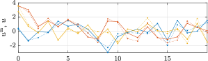
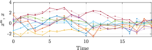
Figure 2: Data collection experiment. (Top) Measured input $u^{\textup{m}}$ with solid line, actual input $u=u^{\textup{m}}-e_{u}$ with dotted line. (Bottom) Measured state $x^{\textup{m}}$ with solid line, actual input $x=x^{\textup{m}}-e_{x}$ with dotted line.

We assume to know that each errors $e_{x}$ and $e_{u}$ satisfy $|e_{x}|^{2}\leq\bar{e}_{x}$ and $|e_{u}|^{2}\leq\bar{e}_{u}$ for some $\bar{e}_{x}\geq 0$ and $\bar{e}_{u}\geq 0$. The quantities of the experiment are depicted in Figure 2, for $\bar{e}_{x}=1$ and $\bar{e}_{u}=1$, $T=20$. Figure 2 shows significant discrepancies between the measured and actual signals. By converting these instantaneous bounds into an energy bound as in Remark 1, we obtain $\Theta=T(2\bar{e}_{x}+\bar{e}_{u})I_{17}$; we also obtain $\theta=2\bar{e}_{x}+\bar{e}_{u}$, see Remark 1 and (15). For this $\Theta$ and $\theta$, (28) was not feasible whereas (31) was. The controller designed with (31) is

$$K=\left[\begin{smallmatrix}-0.0587&-0.1445&0.5473&-0.2702&0.5436&-0.5095&0.4531\\ 0.4209&-0.1096&-0.9401&0.1420&-0.3647&-0.4587&-0.7077\\ -0.0650&1.0126&-2.0646&-0.3754&-0.7337&1.3682&-0.8806\\ \end{smallmatrix}\right]$$

and the resulting closed-loop solutions are in Figure 3.

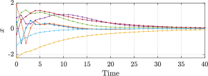
Figure 3: Closed loop of (7) and $u=Kx$, where $K$ is designed by (31).

We now evaluate the performance of the two previous approaches quantitatively, given the same $\bar{e}_{x}$ and $\bar{e}_{u}$. To do so, we follow the type of analysis in [11], to which we refer the reader for more details. Consider different numbers of data points $T\in$ $\{10,$ $20,$ $30,$ $40,$ $50,$ $60,$ $70,$ $80,$ $90,$ $100\}$ and different bounds $\theta\in$ $\{10^{-6},$ $10^{-5},$ $10^{-4},$ $10^{-3},$ $10^{-2},$ $10^{-1},$ $10^{0}\}$. Based on these values of $\theta$, we set $\bar{e}_{x}=\bar{e}_{u}=\theta/3$ so that for each $e_{x}$, $|e_{x}|\leq\sqrt{\bar{e}_{x}}\in$ $\{0.0006,$ $0.0018,$ $0.0058,$ $0.0183,$ $0.0577,$ $0.1826,$ $0.5774\}$, and $\Theta=T\theta I$. For each of these pairs $(T,\theta)$, we randomly generate 20 data sequences; for each data sequence, apply (28) in Theorem 1 and (31) in Theorem 2; then count the number $n_{\textup{feas}}$ of instances when (28) and (31) are feasible. For both cases, we plot the ratio $n_{\textup{feas}}/20\in[0,1]$ in Figure 4 as a function of $(T,\theta)$, with a logarithmic scale for $\theta$. In line with [11], Figure 4 shows that it is more convenient to employ the instantaneous bound directly together with the sufficient condition in Theorem 2, rather than convert it into an energy bound to use the necessary and sufficient condition in Theorem 1. The downside of Theorem 2 over Theorem 1 is that the former involves $T$ more decision variables, but this is hardly an issue unless $T$ is quite large.

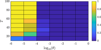
Figure 4: Ratio of $n_{\textup{feas}}/20\in[0,1]$ as a function of $(T,\log_{10}(\theta))$ for (28) (top) and (31) (bottom), with “good” regions in yellow.

VII Conclusions

We have addressed the problem of designing a state-feedback controller based only on noisy data. Specific to this work is that we have considered the setting where input and state are affected by additive measurements errors with both energy and instantaneous bounds. We have provided two linear matrix inequalities for the design of a controller that asymptotically stabilizes all systems consistent with the data points and the respective energy or instantaneous bounds. For the energy bound, the linear matrix inequality is actually equivalent to robust stabilization. Numerical examples have validated these results and provided a caveat for when energy bounds are derived by converting instantaneous ones.

References

- [1] E. Fogel, “System identification via membership set constraints with energy constrained noise,” IEEE Trans. Autom. Contr., vol. 24, no. 5, pp. 752–758, 1979.
- [2] C. De Persis and P. Tesi, “Formulas for data-driven control: Stabilization, optimality, and robustness,” IEEE Trans. Autom. Contr., vol. 65, no. 3, pp. 909–924, 2020.
- [3] J. Berberich, C. W. Scherer, and F. Allgöwer, “Combining prior knowledge and data for robust controller design,” IEEE Trans. Autom. Contr., vol. 68, no. 8, pp. 4618 – 4633, 2023.
- [4] J. Coulson, J. Lygeros, and F. Dörfler, “Distributionally robust chance constrained data-enabled predictive control,” IEEE Trans. Autom. Contr., vol. 67, no. 7, pp. 3289–3304, 2021.
- [5] H. J. van Waarde, M. K. Camlibel, and M. Mesbahi, “From noisy data to feedback controllers: Nonconservative design via a matrix S-lemma,” IEEE Trans. Autom. Contr., vol. 67, no. 1, pp. 162–175, 2022.
- [6] F. Celi, G. Baggio, and F. Pasqualetti, “Closed-form and robust expressions for data-driven LQ control,” Ann. Rev. Contr., vol. 56, p. 100916, 2023.
- [7] T. Söderström, “Why are errors-in-variables problems often tricky?” in Eur. Contr. Conf., 2003, pp. 802–807.
- [8] V. Cerone, D. Piga, and D. Regruto, “Set-membership error-in-variables identification through convex relaxation techniques,” IEEE Trans. Autom. Contr., vol. 57, no. 2, pp. 517–522, 2011.
- [9] T. Söderström, Errors-in-variables methods in system identification. Springer, 2018.
- [10] D. P. Bertsekas and I. B. Rhodes, “Recursive state estimation for a set-membership description of uncertainty,” IEEE Trans. Autom. Contr., vol. 16, no. 2, pp. 117–128, 1971.
- [11] A. Bisoffi, C. De Persis, and P. Tesi, “Trade-offs in learning controllers from noisy data,” Sys. & Contr. Lett., vol. 154, p. 104985, 2021.
- [12] ——, “Data-driven control via Petersen’s lemma,” Automatica, vol. 145, p. 110537, 2022.
- [13] J. Miller, T. Dai, and M. Sznaier, “Data-driven stabilizing and robust control of discrete-time linear systems with error in variables,” arXiv preprint arXiv:2210.13430, 2022.
- [14] L. Li, A. Bisoffi, C. De Persis, and N. Monshizadeh, “Controller synthesis from noisy-input noisy-output data,” 2024, arXiv preprint arXiv:2402.02588.
- [15] R. A. Horn and C. R. Johnson, Matrix Analysis. Cambridge University Press, 2013.
- [16] P. Albertos and A. Sala, Multivariable control systems: an engineering approach. Springer, 2004.