Stochastic theta methods for free stochastic differential equations

Abstract

We introduce free probability analogues of the stochastic theta methods for free stochastic differential equations, which generalize the free Euler-Maruyama method introduced by Schlüchtermann and Wibmer [27]. Under some mild conditions, we prove the strong convergence and exponential stability in mean square of the numerical solution. The free stochastic theta method with $\theta=1$ can inherit the exponential stability of original equations for any given step size. Our method can offer better stability and efficiency than the free Euler-Maruyama method. Moreover, numerical results are reported to confirm these theoretical findings.

AMS subject classification: 65C30, 60H35, 46L54, 46L55

Key Words: free stochastic differential equations, stochastic theta methods, strong convergence, exponential stability in mean square

1 Introduction

Free probability, introduced by Voiculescu [29], is a non-commutative analogue of classical probability, where the random variables are considered as operators in a non-commutative probability space. Free stochastic calculus was initiated by Biane and Speicher [21, 4, 5, 28] and is devoted to studying the operator-valued process. Let $(\mathscr{F},\psi)$ be a non-commutative probability space, where $\mathscr{F}$ is a von Neumann algebra and $\psi:\mathscr{F}\to\mathbb{C}$ is a faithful unital normal trace on $\mathscr{F}.$ We will consider the following free analogue of the stochastic differential equation [18]:

$${\rm d}U_{t}=\alpha(U_{t}){\rm dt}+\beta(U_{t}){\rm d}W_{t}\gamma(U_{t}),$$ (1.1)

where $\{U_{t}\}_{t}$ is a $\mathscr{F}$-valued process, $\{W_{t}\}_{t}$ is the free Brownian motion [4] on $\mathscr{F}$, and $\alpha,\beta,\gamma$ are real-valued functions. One motivation for studying free stochastic differential equations (free SDEs) dates back to stochastic calculus on matrices. Let $\{U_{t}^{(N)}\}_{t}$ be a $M_{N}(\mathbb{C})$-valued process, where $M_{N}(\mathbb{C})$ is the set of all $N\times N$ matrices, and let $\{W_{t}^{(N)}\}_{t}$ be the ${\rm GUE}_{N}$ Brownian motion [19]. Then the free SDEs (1.1) can be considered as the large $N$-limit of the following matrix-valued SDEs:

$${\rm d}U_{t}^{(N)}=\alpha(U_{t}^{(N)}){\rm dt}+\beta(U_{t}^{(N)}){\rm d}W_{t}^{(N)}\gamma(U_{t}^{(N)}).$$ (1.2)

We refer to [19] for the proof of convergence of $\{W_{t}^{(N)}\}_{t}$ to the free Brownian motion $\{W_{t}\}_{t}$. Hence, solving free SDEs (1.1) helps to study the limiting eigenvalue distribution of $U_{t}^{(N)}$ [18, 19, 15].

However, finding the exact solution to free SDEs is a daunting task due to the non-commutativity of the operators. By consulting the classical SDEs, one can provide numerical solutions to free SDEs as a means of approximating analytical solutions. For classical SDEs, there are many experts contributing themselves to exploring various numerical methods; see [20, 23, 12, 11, 17]. On the contrary, studying the numerical methods for free SDEs is an emerging field. Biane and Speicher initially developed an Euler scheme to approximate the solution of a peculiar free SDE in the operator norm [5]. Very recently, Schlüchtermann and Wibmer introduced a free analogue of the Euler-Maruyama method (free EM) for the free SDEs (1.1) [27]. More precisely, for $P\in\mathbb{N},$ let $0=t_{0}\leq t_{1}\leq\cdots\leq t_{P}=T$ be a partition of $[0,T]$ with a constant step size $h=T/P,$ define

$$U_{n+1}=U_{n}+\alpha(U_{n})h+\beta(U_{n})\Delta W_{n}\gamma(U_{n}),\ n=0,1,\ldots,P-1,$$ (1.3)

with the starting value $U_{0},$ where $\Delta W_{n}:=W_{t_{n+1}}-W_{t_{n}}.$ $U_{n}$ is called the numerical approximation of $U_{t}$ at time point $t_{n}$. They proved the strong and weak convergence of free EM.

Motivated by their pioneering work and the work of stochastic theta methods applied on classical SDEs [3, 7, 10, 16, 13, 31], we introduce the following free analogue of stochastic theta methods (free STMs): let $0\leq\theta\leq 1,$ define

$$\bar{U}_{n+1}=\bar{U}_{n}+(1-\theta)\alpha(\bar{U}_{n})h+\theta\alpha(\bar{U}_{n+1})h+\beta(\bar{U}_{n})\Delta W_{n}\gamma(\bar{U}_{n}),\ n=0,1,\ldots,P-1,$$ (1.4)

with the starting value $U_{0}.$ Note that the free STMs reduce to the free EM when $\theta=0.$ Since it is an implicit method for $0<\theta\leq 1$, it requires some conditions for the existence of the numerical solution. For instance, suppose that $\alpha$ is operator Lipschitz, i.e., there is a constant $L_{0}>0$ such that

$$\left\|\alpha(U)-\alpha(V)\right\|\leq L_{0}\left\|U-V\right\|$$

for any self-adjoint element $U,V\in\mathscr{F}.$ Then $\bar{U}_{n}$ uniquely exists if $h<1/(\theta L_{0})$ by a fixed point argument. Our paper contributes two main results:

First, we will prove the strong convergence property of the free STMs under some mild conditions. Just as in the classical case, strong convergence is generally used to judge the validity of numerical methods [8]. Suppose that $\alpha,\beta,$ and $\gamma$ are real-valued functions with some operator Lipschitz properties, then the numerical solution generated by the free STMs (1.4) strongly converges to the exact solution to the free SDEs $\eqref{eq:fSDE-0}$ with order $1/2$; see Theorem 2. Our main tools are free Itô formula and free Burkholder-Gundy inequality [4, 2]. The second result is devoted to the stability of the numerical solution, which is essential to confirming whether the numerical method can inherit the stability of original equations. To the best of our knowledge, the stability of the exact and numerical solution to free SDEs have not been studied. Suppose that there exist constants $L^{\prime},\hat{K},\bar{K}>0$ such that ${\rm(a)}\;\psi\left(U\alpha(U)\right)\leq-L^{\prime}\|U\|_{2}^{2},$ ${\rm(b)}\;\|\beta(U)\|_{2}^{2}\cdot\|\gamma(U)\|_{2}^{2}\leq\hat{K}\|U\|^{2}_{2},$ and ${\rm(c)}\;\|\alpha(U)\|_{2}\leq\bar{K}\|U\|_{2}$ for any self-adjoint element $U\in\mathscr{F}.$ Here $L^{2}(\psi)$ is the non-commutative $L^{2}$ space [26] that is the completion of $\mathscr{F}$ with respect to the norm $\|\cdot\|_{2}:=\psi[|\cdot|^{2}]^{1/2},$ where $|U|=(U^{*}U)^{1/2}$ for any $U\in\mathscr{F}.$ If $2L^{\prime}>\hat{K},$ then the numerical solution generated by the free STMs (1.4) is exponentially stable in mean square whenever the step size $0<h<\frac{2L^{\prime}-\hat{K}}{(1-\theta)^{2}\bar{K}};$ see Theorem 6. We emphasize that in the case of $\theta=1,$ which is called the free backward Euler method (free BEM), the numerical solution is exponentially stable for any step size without condition ${\rm(c)}$; see Corollary 1. Hence, it offers better stability and efficiency than free EM. Finally, we verify our results by conducting numerical experiments on several specific free SDEs. As indicated in [27], to implement free STMs (or free EM) as a numerical method on a computer, it is necessary to consider the set of $N\times N$ matrices instead of the abstract von Neumann algebra $\mathscr{F}$ and let $N\to\infty$.

The rest of the paper is organized as follows: Section 2 collects some preliminary results. Section 3 concerns the strong convergence and exponential stability in mean square of the numerical solution, which offer our main results. In the last section, we provide some numerical experiments to verify our theoretical results.

2 Preliminaries

In this section, we collect some results in free probability and free stochastic calculus, and refer to [25, 24] for more details. We will also discuss the solution of free stochastic differential equations, which refers to [18, 22].

2.1 Free probability

A non-commutative probability space $(\mathscr{F},\psi)$ is a von Neumann algebra $\mathscr{F}$, with a faithful unital normal trace $\psi:\mathscr{F}\to\mathbb{C}.$ Here are two examples of non-commutative probability spaces:

1. $(L^{\infty}(\mathbb{R},\mu),\mathbb{E}),$ where $\mu$ is a probability measure supporting on $\mathbb{R},$ and $\mathbb{E}$ is the expecation defined by $\mathbb{E}[f]:=\int_{\mathbb{R}}f(t){\rm d\mu(t)}.$

2. $(M_{N}(\mathbb{C}),{\rm tr}_{N}),$ where $M_{N}(\mathbb{C})$ is the set of $N\times N$ matrices, and ${\rm tr}_{N}:={\rm Tr}/N$ is the normalized trace.

The element $U\in\mathscr{F}$ is called a non-commutative probability random variable, and it is called centered if $\psi(U)=0.$ Instead of ”classical independence”, ”free independence” takes a central role in free probability. Let $\mathscr{F}_{1},\mathscr{F}_{2},\ldots,\mathscr{F}_{m}$ be subsets of $\mathscr{F}.$ Denote $W^{*}(\mathscr{F}_{i})$ by the von Neumann sub-algbera generated by $\mathscr{F}_{i}.$ We call $\mathscr{F}_{1},\mathscr{F}_{2},\ldots,\mathscr{F}_{m}$ are freely independent, if for any centered random variables $U_{j}\in W^{*}(\mathscr{F}_{i_{j}}),i_{j}\in\{1,\ldots,m\},j=1,\ldots,k,$

$$\psi(U_{1}\cdots U_{k})=0,$$

whenever we have $i_{j}\neq i_{j+1}$ for $j=1,\ldots,k-1.$ Roughly speaking, free independence provides a systematic way to calculate the joint distribution of random variables from their marginal distributions. For instance, if $\{U_{1},U_{2}\},\{U_{3}\}$ are freely independent, then $\psi(U_{1}U_{3}U_{2})=\psi(U_{1}U_{2})\cdot\psi(U_{3}).$

A self-adjoint random variable $S\in\mathscr{F}$ is called a semicircular element (or has a semicircular distribution with mean 0 and variance $\sigma^{2}$) [30], if

$$\psi\left(S^{k}\right)=\int_{\mathbb{R}}t^{k}{\rm d\mu_{sc}(t)}$$

for any $k\in\mathbb{N},$ where $\mu_{sc}$ is a probability measure supporting on $\mathbb{R}$ with density ${\rm d\mu_{sc}(t)}=\frac{1}{2\pi\sigma^{2}}\sqrt{4\sigma^{2}-t^{2}}\cdot{\bf 1}_{\{|t|\leq 2\sigma\}}(t){\rm dt}.$

For any $U\in\mathscr{F},$ define

$$\left\|U\right\|_{p}:=\left(\psi\left(|U|^{p}\right)\right)^{1/p}$$

for $1\leq p<\infty,$ where $|U|=(U^{*}U)^{1/2}.$ The completion of $\mathscr{F}$ with respect to the norm $\|\cdot\|_{p}$ is called a non-commutative $L^{p}$ space [26], denoted by $L^{p}(\psi).$

2.2 Free stochastic integral

Let $(\mathscr{F},\psi)$ be a non-commutative probability space, and a filtration $\{\mathscr{F}_{t}\}_{t\geq 0}$ be a family of sub-algebras of $\mathscr{F}$ such that $\mathscr{F}_{s}\subset\mathscr{F}_{t}$ for $s\leq t$. A free stochastic process is a family of elements $\{U_{t}\}_{t\geq 0}$ for which the increments $U_{t}-U_{s}$ are free with respect to the sub-algebra $\mathscr{F}_{s}$. $\{U_{t}\}_{t\geq 0}$ is called adapted to the filtration $\{\mathscr{F}_{t}\}_{t\geq 0}$ if $U_{t}\in\mathscr{F}_{t}$ for all $t\geq 0.$ A family of self-adjoint elements $\{W_{t}\}_{t\geq 0}$ in $\mathscr{F}$ is called a free Brownian motion if it satisfies

1. $W_{0}=0;$

2. The increments $W_{t}-W_{s}$ are free from $\mathscr{W}_{s}$ for all $0\leq s<t$, where $\mathscr{W}_{s}$ is the von Neumann algebra generated by $\{W_{\tau}:0\leq\tau\leq s\}$;

3. The increment $W_{t}-W_{s}$ has a semicircular distribution with mean 0 and variance $t-s$ for all $0\leq s<t$.

It is clear that $\{\mathscr{W}_{t}\}_{t\geq 0}$ is a filtration in $\mathscr{F},$ and the free Brownian motion $\{W_{t}\}_{t\geq 0}$ is adapted to $\{\mathscr{W}_{t}\}_{t\geq 0}.$ Given $T>0,$ suppose that $\beta_{t},\gamma_{t}\in\mathscr{W}_{t}$ and $\|\beta_{t}\|\cdot\|\gamma_{t}\|\in L^{2}([0,T])$. Let $0=t_{0}\leq t_{1}\leq\cdots\leq t_{n}=T$ be a partition of $[0,T]$, denoted by $\Delta_{n}$. Consider the finite sum

$$I_{n}:=\sum_{i=1}^{n}\beta_{t_{i-1}}(W_{t_{i}}-W_{t_{i-1}})\gamma_{t_{i-1}}.$$

It is known [4] that $I_{n}$ converges in the operator norm as $d(\Delta_{n})\rightarrow 0,$ where $d(\Delta_{n}):=\max_{1\leq k\leq n}(t_{k}-t_{k-1}),$ and the convergence does not depend on the partition. Hence, we have the following definition:

Definition 1 (Free stochastic integral [4, 18]).

Given $T>0,$ suppose that $\beta_{t},\gamma_{t}\in\mathscr{W}_{t}$ and $\|\beta_{t}\|\cdot\|\gamma_{t}\|\in L^{2}([0,T])$. The free stochastic integral of $\{\beta_{t}\}_{t\geq 0}$ and $\{\gamma_{t}\}_{t\geq 0}$ is defined as the limit (in the operator norm) of $I_{n}$, denoted by

$$I=\int_{0}^{T}\beta_{t}{\rm d}W_{t}\gamma_{t}.$$

A key ingredient to show the convergence of $I_{n}$ is the following free Burkholder-Gundy (B-G) inequality [4], which will be used frequently in our paper:

$$\left\|\int_{0}^{T}\beta_{t}{\rm d}W_{t}\gamma_{t}\right\|\leq 2\sqrt{2}\left(\int_{0}^{T}\|\beta_{t}\|^{2}\cdot\|\gamma_{t}\|^{2}{\rm dt}\right)^{1/2},$$ (2.1)

and for the $L^{2}(\psi)$-norm, we have the following free $L^{2}(\psi)$-isometry:

$$\left\|\int_{0}^{T}\beta_{t}{\rm d}W_{t}\gamma_{t}\right\|_{2}\leq\left(\int_{0}^{T}\|\beta_{t}\|^{2}_{2}\cdot\|\gamma_{t}\|^{2}_{2}{\rm dt}\right)^{1/2}.$$ (2.2)

Another important tool is the free Itô formula [4, 2]. In terms of formal rules, it can be written as follows:

$$\begin{split}&\alpha_{t}{\rm dt}\cdot\beta_{t}{\rm dt}=\alpha_{t}{\rm dt}\cdot\beta_{t}{\rm d}W_{t}\gamma_{t}=\alpha_{t}{\rm d}W_{t}\beta_{t}\cdot\gamma_{t}{\rm dt}=0,\\ &\alpha_{t}{\rm d}W_{t}\beta_{t}\cdot\gamma_{t}{\rm d}W_{t}\zeta_{t}=\psi\left(\beta_{t}\gamma_{t}\right)\alpha_{t}\zeta_{t}{\rm dt}\end{split}$$ (2.3)

for any $\alpha_{t},\beta_{t},\gamma_{t},\zeta_{t}\in\mathscr{W}_{t}.$

2.3 Free stochastic differential equation

Given functions $\alpha,\beta^{i},\gamma^{i}:\mathbb{R}\rightarrow\mathbb{R},i=1,2,\ldots,k,$ $k\in\mathbb{N}.$ A general form of free SDEs with an initial value of $U_{0}\in\mathscr{F}^{sa}$ is given by [18]

$${\rm d}U_{t}=\alpha(U_{t}){\rm dt}+\sum_{i=1}^{k}\beta^{i}(U_{t}){\rm d}W_{t}\gamma^{i}(U_{t}),$$ (2.4)

which is a convenient shortcut notation for the following integral equation:

$$U_{t}=U_{0}+\int_{0}^{t}\alpha(U_{s}){\rm ds}+\sum_{i=1}^{k}\int_{0}^{t}\beta^{i}(U_{s}){\rm d}W_{s}\gamma^{i}(U_{s}).$$ (2.5)

We denote the set of all self-adjoint elements in $\mathscr{F}$ by $\mathscr{F}^{sa}.$

Motivated by the classical SDEs [22], we have the following definition for the solution of free SDEs:

Definition 2.

For $T>0,$ a free stochastic process $\{U_{t}\}_{0\leq t\leq T}$ adapted to the filtration $\{\mathscr{W}_{t}\}_{t\geq 0}$ is called a (strong) solution to the free SDEs (2.4), if the following conditions hold:

1. $U_{t}\in\mathscr{F}^{sa}$ for all $0\leq t\leq T$;

2. $\|\alpha(U_{t})\|\in L^{1}([0,T])$ and $\|\beta^{i}(U_{t})\|\cdot\|\gamma^{i}(U_{t})\|\in L^{2}([0,T]),i=1,2,\ldots,k$;

3. $U_{t}$ fulfills equation (2.5) for all $0\leq t\leq T.$

Recall that a function $f:\mathbb{R}\to\mathbb{R}$ is called locally operator Lipschitz, if it is a locally bounded, measurable function such that for all $M>0,$ there is a constant $L_{f}(M)>0$ such that

$$\left\|f(U)-f(V)\right\|\leq L_{f}(M)\left\|U-V\right\|$$

for $U,V\in\mathscr{F}^{sa}$ and $\|U\|,\|V\|\leq M.$ It was shown by Kargin that there exists a local solution to the free SDEs (2.4) if $\alpha,\beta^{i},$ and $\gamma^{i}$ $(i=1,2,\ldots,k)$ are locally operator Lipschitz. More precisely, we have the following theorem:

Theorem 1 (Theorem 3.1, [18]).

Suppose that $\alpha,\beta,$ and $\gamma$ are locally operator Lipschitz functions. Then there exist a sufficient small $T_{0}>0$ and a family of operators $U_{t}$ defined for all $t\in[0,T_{0})$, such that $U_{t}$ is a unique solution to (2.4) for $t<T_{0}.$

Moreover, it is clear that the solution $\{U_{t}\}_{t\in[0,T_{0})}$ is uniformly bounded, i.e., there exists a constant $A>0,$ such that

$$\sup_{0\leq t<T_{0}}\|U_{t}\|\leq A.$$

However, the existence of the global solution to (2.4) is not clear by assuming that $\alpha,\beta,$ and $\gamma$ are locally operator Lipschitz. We provide some examples for which the global solution exists.

1. Free Ornstein-Uhlenbeck process [18]:

   $${\rm d}U_{t}=\theta U_{t}{\rm dt}+\sigma{\rm d}W_{t},\;\theta,\sigma\in\mathbb{R}.$$

2. Geometric Brownian motion I [18]:

   $${\rm d}U_{t}=\theta U_{t}{\rm dt}+\sqrt{U_{t}}{\rm d}W_{t}\sqrt{U_{t}},\;\theta\in\mathbb{R}.$$

3. Geometric Brownian motion II [18]:

   $${\rm d}U_{t}=\theta U_{t}{\rm dt}+U_{t}{\rm d}W_{t}+{\rm d}W_{t}U_{t},\;\theta\in\mathbb{R}.$$

4. Free CIR-process [9, 6]:

   $${\rm d}U_{t}=(\alpha-\beta U_{t}){\rm dt}+\frac{\sigma}{2}\sqrt{U_{t}}{\rm d}W_{t}+\frac{\sigma}{2}{\rm d}W_{t}\sqrt{U_{t}},$$

   where $\alpha,\beta,\sigma>0$ and satisfy the Feller condition $2\alpha\geq\sigma^{2}.$

(a), (c), and (d) can be generalized to the following model:

$${\rm d}U_{t}=\alpha(U_{t}){\rm dt}+\sum_{i=1}^{k}\left(\beta^{i}(U_{t}){\rm d}W_{t}+{\rm d}W_{t}\gamma^{i}(U_{t})\right).$$

If $\alpha,\beta^{i},$ and $\gamma^{i}$ $(i=1,2,\ldots,k)$ are operator Lipschitz, then there exists a unique global solution. The proof is similar to the classical case, and we omit the details.

3 Free analogue of the stochastic theta methods

Inspired by the pioneering work [27], we can define the free analogue of stochastic theta methods (free STMs). Recall that $\alpha,\beta^{i},$ and $\gamma^{i}$ $(i=1,2,\ldots,k)$ are real-valued functions.

Definition 3.

Given $T>0$ and $\theta\in[0,1].$ For $P\in\mathbb{N},$ let $0=t_{0}\leq t_{1}\leq\cdots\leq t_{P}=T$ be a partition of $[0,T]$ with constant step size $h=T/P.$ Define the one step free STMs approximation $\bar{U}_{n}$ of the solution $U_{t}$ to the free SDEs (2.4) on $[0,T]$ by

$$\bar{U}_{n+1}=\bar{U}_{n}+(1-\theta)\alpha(\bar{U}_{n})h+\theta\alpha(\bar{U}_{n+1})h+\sum_{i=1}^{k}\beta^{i}(\bar{U}_{n})\Delta W_{n}\gamma^{i}(\bar{U}_{n}),$$ (3.1)

$n=0,1,\ldots,P-1,$ with start value $\bar{U}_{0}=U_{0}\in\mathscr{F}^{sa}$ and where $\Delta W_{n}:=W_{t_{n+1}}-W_{t_{n}}$ is the increment of the free Brownian motion $\{W_{t}\}_{t\geq 0}.$ Here $\bar{U}_{n}\in\mathscr{F}^{sa}$ is called the numerical approximation of $U_{t}$ at the time point $t_{n}.$

For $\bar{U}_{n}$ to be self-adjoint, it requires that the sum $\sum_{i=1}^{k}\beta^{i}(\bar{U}_{n})\Delta W_{n}\gamma^{i}(\bar{U}_{n})$ is self-adjoint for all $n.$ If $\theta=0,$ free STM reduces to the free Euler-Maruyama method (free EM) introduced in [27], and $\bar{U}_{n+1}$ is explicitly determined by $\bar{U}_{n}.$ However, for $0<\theta\leq 1,$ Equation (3.1) is implicit. Since the locally operator Lipschitz property of $\alpha,\beta^{i},$ and $\gamma^{i}$ is not enough to guarantee the well-posedness of free SDEs and free STMs. We require the following assumption:

Assumption 1 (Well-posedness of free SDEs and free STMs).

Given $T>0$, we assume that there exists a unique solution $\{U_{t}\}_{t\in[0,T]}$ to the free SDEs (2.4), satisfying $\sup_{t\in[0,T]}\|U_{t}\|<\infty.$ Moreover, suppose that there exists a unique solution $\{\bar{U}_{n}\}_{n=0,1,\ldots,P}$ to the free STMs (3.1), such that $\{\bar{U}_{n}\}_{n=0,1,\ldots,P}$ is adapted to $\{\mathscr{W}_{t_{n}}\}_{n=0,1,\ldots,P}.$

Remark 1.

We remark that one simple condition for the well-posedness of the free STMs can be easily obtained by using a fixed-point argument. Define

$$F(U):=\bar{U}_{n}+(1-\theta)\alpha(\bar{U}_{n})h+\theta\alpha(U)h+\sum_{i=1}^{k}\beta^{i}(\bar{U}_{n})\Delta W_{n}\gamma^{i}(\bar{U}_{n}).$$

We assume that the function $\alpha:\mathbb{R}\rightarrow\mathbb{R}$ is operator Lipschitz with Lipschitz constant $L_{0}.$ If $h<1/(\theta L_{0})$, then we have

$$\|F(U)-F(V)\|\leq\theta h\|\alpha(U)-\alpha(V)\|\leq L_{0}\theta h\|U-V\|<\|U-V\|,$$

for any $U,V\in\mathscr{F}^{sa}.$ Hence, $F(\cdot)$ is a contraction, and the fixed-point theorem implies the existence and uniqueness of $\bar{U}_{n+1}$. Moreover, define $f:\mathbb{R}\to\mathbb{R}$ by

$$f(x):=x-\theta h\alpha(x).$$

Then,

$$f(x_{1})-f(x_{2})\geq(1-\theta L_{0}h)(x_{1}-x_{2})$$

for $x_{1}>x_{2}.$ Hence, $f$ is uniformly monotone for $h<1/(\theta L_{0})$, and the inverse $f^{-1}$ exists for every $h<1/(\theta L_{0})$. By the functional calculus, we have

$$\bar{U}_{n+1}=f^{-1}\left(\bar{U}_{n}+(1-\theta)\alpha(\bar{U}_{n})h+\sum_{i=1}^{k}\beta^{i}(\bar{U}_{n})\Delta W_{n}\gamma^{i}(\bar{U}_{n})\right).$$

Therefore, $\{\bar{U}_{n}\}_{n=0,1,\ldots,P}$ is adapted to $\{\mathscr{W}_{t_{n}}\}_{n=0,1,\ldots,P}$ whenever the step size $h<1/(\theta L_{0}).$

For simplicity, we assume $k=1$ in the sequel. For the convergence and stability of the free STMs, we need the following additional assumption:

Definition 4 ([1, 27]).

A function $f:\mathbb{R}\rightarrow\mathbb{R}$ is called locally operator Lipschitz in the $L^{2}(\psi)$ norm, if it is a locally bounded, measurable function such that for all $M>0,$ there is a constant $L_{f}(M)>0$ such that

$$\left\|f(U)-f(V)\right\|_{2}\leq L_{f}(M)\left\|U-V\right\|_{2}$$

for $U,V\in\mathscr{F}^{sa}$ and $\left\|U\right\|_{2},\left\|V\right\|_{2}\leq M.$

Moreover, $f$ is called operator Lipschitz in the $L^{2}(\psi)$ norm, if there is a constant $L_{f}>0$ such that

$$\left\|f(U)-f(V)\right\|_{2}\leq L_{f}\left\|U-V\right\|_{2}$$

for $U,V\in\mathscr{F}^{sa}.$

Assumption 2.

We assume that $\alpha$ is operator Lipschitz in the $L^{2}(\psi)$ norm, and $\beta,\gamma$ are locally operator Lipschitz in the $L^{2}(\psi)$ norm.

It is clear that there exists a constant $K_{\alpha}>0$, only depending on $L_{\alpha}$ and $U_{0},$ such that for any $U\in\mathscr{F}^{sa},$

$$\left\|\alpha(U)\right\|_{2}\leq K_{\alpha}\left(1+\left\|U\right\|_{2}\right).$$ (3.2)

We will also frequently use the following condition:

$$\left\|\alpha(U)\right\|^{2}_{2}\leq K^{\prime}_{\alpha}\left(1+\left\|U\right\|^{2}_{2}\right),$$ (3.3)

where $K^{\prime}_{\alpha}>0$ is a constant only depending on $L_{\alpha}$ and $U_{0}.$ Moreover, there exist constants $K_{\beta}(M),K^{\prime}_{\beta}(M)>0$, only depending on $L_{\beta}(M)$ and $U_{0},$ such that for any $U\in\mathscr{F}^{sa}$ and $\left\|U\right\|_{2}\leq M,$

$$\left\|\beta(U)\right\|_{2}\leq K_{\beta}(M)\left(1+\left\|U\right\|_{2}\right),\;\text{and}\;\left\|\beta(U)\right\|^{2}_{2}\leq K^{\prime}_{\beta}(M)\left(1+\left\|U\right\|^{2}_{2}\right).$$ (3.4)

And similar results hold for $\gamma.$

In the rest of this section, we will use the following notations:

$$\begin{split}L_{M}&:=\max\{L_{\alpha},L_{\beta}(M),L_{\gamma}(M)\},\\ K_{M}&:=\max\{K_{\alpha},K_{\beta}(M),K_{\gamma}(M)\},K^{\prime}_{M}:=\max\{K^{\prime}_{\alpha},K^{\prime}_{\beta}(M),K^{\prime}_{\gamma}(M)\}.\end{split}$$ (3.5)

3.1 Uniformly boundness of the numerical solutions

We introduce a piecewise constant process $\{\bar{U}_{t}\}_{t\in[0,T]}$ defined by

$$\bar{U}_{t}:=\bar{U}_{n}$$ (3.6)

for $t_{n}\leq t<t_{n+1},$ where $\{\bar{U}_{n}:n=0,1,\ldots,P\}$ is a numerical solution on $[0,T]$ given by (3.1). Suppose that $\{U_{t}\}_{t\in[0,T]}$ is a solution to the free SDEs (2.4), it is not difficult to show that $\|U_{t}\|_{2}$ is uniformly bounded; see [27, Remark 3.3].

Proposition 1.

Fix $0<C_{0}<1.$ For $0<\theta\leq 1,$ suppose that Assumption 1, 2 hold. Define $\tilde{A}=A+2,$ where $A=\sup_{t\in[0,T]}\|U_{t}\|_{2}^{2}.$ Denote $K^{\prime}_{0}:=\max\{K^{\prime}_{\alpha},K^{\prime}_{\beta\gamma}(\tilde{A})\}.$ Then there exists a time point $0<\tilde{T}\leq T,$ such that

$$\sup_{t\in[0,\tilde{T}]}\left\|\bar{U}_{t}\right\|_{2}^{2}\leq\tilde{A}$$ (3.7)

whenever $0<h\leq\frac{C_{0}}{\theta(1+K^{\prime}_{0})}.$

Proof.

Since $\left\|U_{0}\right\|_{2}^{2}\leq A<\tilde{A},$ there exists a time point $T^{(h)}\in(0,T],$ depending on $h$, such that $\|\bar{U}_{t}\|_{2}^{2}\leq\tilde{A}$ for all $t\in[0,T^{(h)}].$ Considering a partition

$$0=t_{0}\leq t_{1}\leq\cdots\leq t_{n_{0}}=T^{(h)}\leq t_{n_{0}+1}\leq\cdots\leq t_{P}=T.$$

Without losing generality, we may assume that $\|\bar{U}_{t_{n_{0}+1}}\|_{2}^{2}>\tilde{A}.$

For $n=0,1,\ldots,n_{0},$ moving the term $\theta\alpha(\bar{U}_{n+1})h$ in (3.1) to the left hand side, we obtain

$$\bar{U}_{n+1}-\theta\alpha(\bar{U}_{n+1})h=\bar{U}_{n}+(1-\theta)\alpha(\bar{U}_{n})h+\beta(\bar{U}_{n})\Delta W_{n}\gamma(\bar{U}_{n}).$$ (3.8)

On one hand, thanks to $2\psi(UV)\leq 2\|U\|_{2}\|V\|_{2}\leq\|U\|_{2}^{2}+\|V\|_{2}^{2},$ we have

$$2\psi\left(\bar{U}_{n+1}\alpha(\bar{U}_{n+1})\right)\leq 2\left\|\bar{U}_{n+1}\right\|_{2}\cdot\left\|\alpha(\bar{U}_{n+1})\right\|_{2}\leq\left\|\bar{U}_{n+1}\right\|_{2}^{2}+\left\|\alpha(\bar{U}_{n+1})\right\|_{2}^{2}.$$

Then, it follows that

$$\begin{split}\left\|\bar{U}_{n+1}-\theta\alpha(\bar{U}_{n+1})h\right\|_{2}^{2}&=\left\|\bar{U}_{n+1}\right\|_{2}^{2}-2\theta h\psi\left(\bar{U}_{n+1}\alpha(\bar{U}_{n+1})\right)+\theta^{2}h^{2}\left\|\alpha(\bar{U}_{n+1})\right\|_{2}^{2}\\ &\geq\left\|\bar{U}_{n+1}\right\|_{2}^{2}-\theta h\left\|\alpha(\bar{U}_{n+1})\right\|_{2}^{2}-\theta h\left\|\bar{U}_{n+1}\right\|_{2}^{2}\\ &\geq\left(1-\theta h-K^{\prime}_{0}\theta h\right)\left\|\bar{U}_{n+1}\right\|_{2}^{2}-K^{\prime}_{0}\theta h.\end{split}$$ (3.9)

On the other hand,

$$\begin{split}&\left\|\bar{U}_{n}+(1-\theta)\alpha(\bar{U}_{n})h+\beta(\bar{U}_{n})\Delta W_{n}\gamma(\bar{U}_{n})\right\|_{2}^{2}\\ &\quad\quad=\left\|\bar{U}_{n}\right\|_{2}^{2}+(1-\theta)^{2}h^{2}\left\|\alpha(\bar{U}_{n})\right\|_{2}^{2}+\left\|\beta(\bar{U}_{n})\Delta W_{n}\gamma(\bar{U}_{n})\right\|_{2}^{2}\\ &\quad\quad\quad+2(1-\theta)h\psi\left(\bar{U}_{n}\alpha(\bar{U}_{n})\right)+2\psi\left(\bar{U}_{n}\beta(\bar{U}_{n})\Delta W_{n}\gamma(\bar{U}_{n})\right)\\ &\quad\quad\quad+2(1-\theta)h\psi\left(\alpha(\bar{U}_{n})\beta(\bar{U}_{n})\Delta W_{n}\gamma(\bar{U}_{n})\right).\end{split}$$ (3.10)

Since $\bar{U}_{n}$ is freely independent from $\Delta W_{n},$ we have

$$\psi\left(\bar{U}_{n}\beta(\bar{U}_{n})\Delta W_{n}\gamma(\bar{U}_{n})\right)=\psi\left(\bar{U}_{n}\beta(\bar{U}_{n})\gamma(\bar{U}_{n})\right)\cdot\psi\left(\Delta W_{n}\right)=0,$$

where we have used $\psi\left(\Delta W_{n}\right)=0.$ Similarly, we have $\psi\left(\alpha(\bar{U}_{n})\beta(\bar{U}_{n})\Delta W_{n}\gamma(\bar{U}_{n})\right)=0.$ Moreover,

$$\begin{split}\left\|\beta(\bar{U}_{n})\Delta W_{n}\gamma(\bar{U}_{n})\right\|_{2}^{2}&=\psi\left(\beta(\bar{U}_{n})\Delta W_{n}\gamma(\bar{U}_{n})\beta(\bar{U}_{n})\Delta W_{n}\gamma(\bar{U}_{n})\right)\\ &=\psi\left(\beta(\bar{U}_{n})\gamma(\bar{U}_{n})\beta(\bar{U}_{n})\gamma(\bar{U}_{n})\right)\cdot\psi\left(\Delta W_{n}\Delta W_{n}\right).\end{split}$$

Note that

$$\psi\left(\Delta W_{n}\Delta W_{n}\right)=\left\|\Delta W_{n}\right\|_{2}^{2}=\left\|\int_{t_{n}}^{t_{n+1}}{\rm d}W_{s}\right\|_{2}^{2}=\int_{t_{n}}^{t_{n+1}}1{\rm ds}=h.$$

Thus (see also [27, Lemma 6.5]),

$$\begin{split}\left\|\beta(\bar{U}_{n})\Delta W_{n}\gamma(\bar{U}_{n})\right\|_{2}^{2}&=\psi\left(\beta(\bar{U}_{n})\gamma(\bar{U}_{n})\beta(\bar{U}_{n})\gamma(\bar{U}_{n})\right)h\\ &\leq\left\|\beta(\bar{U}_{n})\gamma(\bar{U}_{n})\right\|_{2}^{2}h\\ &\leq K^{\prime}_{0}\left(1+\left\|\bar{U}_{n}\right\|_{2}^{2}\right)h,\end{split}$$ (3.11)

where we note that the product of two locally operator Lipschitz functions is still locally operator Lipschitz [1]. Putting the above estimations together, for $n=0,1,\ldots,n_{0},$

$$\begin{split}\eqref{eq:1}&\leq\left\|\bar{U}_{n}\right\|_{2}^{2}+(1-\theta)^{2}h^{2}\left\|\alpha(\bar{U}_{n})\right\|_{2}^{2}+K^{\prime}_{0}\left(1+\left\|\bar{U}_{n}\right\|_{2}^{2}\right)h\\ &\quad+2(1-\theta)h\psi\left(\bar{U}_{n}\alpha(\bar{U}_{n})\right)\\ &\leq\left\|\bar{U}_{n}\right\|_{2}^{2}+(1-\theta)^{2}h^{2}\left\|\alpha(\bar{U}_{n})\right\|_{2}^{2}+K^{\prime}_{0}\left(1+\left\|\bar{U}_{n}\right\|_{2}^{2}\right)h\\ &\quad+(1-\theta)h\left\|\bar{U}_{n}\right\|_{2}^{2}+(1-\theta)h\left\|\alpha(\bar{U}_{n})\right\|_{2}^{2}\\ &=f\left(\theta,h,K^{\prime}_{0}\right)+\left[1+g\left(\theta,h,K^{\prime}_{0}\right)\right]\cdot\left\|\bar{U}_{n}\right\|_{2}^{2},\end{split}$$ (3.12)

where we denote $f\left(\theta,h,K^{\prime}_{0}\right):=\left[1+(1-\theta)+(1-\theta)^{2}h\right]K^{\prime}_{0}h$ and $g\left(\theta,h,K^{\prime}_{0}\right)=(1-\theta)h+f\left(\theta,h,K^{\prime}_{0}\right).$ Combining (3.8), (3.9), and (3.12), we obtain (note that $h\leq\frac{C_{0}}{\theta(1+K^{\prime}_{0})}<\frac{1}{\theta(1+K^{\prime}_{0})}$)

$$\left(1-\theta h-K^{\prime}_{0}\theta h\right)\left\|\bar{U}_{n+1}\right\|_{2}^{2}-K^{\prime}_{0}\theta h\leq f\left(\theta,h,K^{\prime}_{0}\right)+\left[1+g\left(\theta,h,K^{\prime}_{0}\right)\right]\cdot\left\|\bar{U}_{n}\right\|_{2}^{2},$$

which is equivalent to

$$\begin{split}\left\|\bar{U}_{n+1}\right\|_{2}^{2}&\leq\frac{f\left(\theta,h,K^{\prime}_{0}\right)+K^{\prime}_{0}\theta h}{1-\theta h-K^{\prime}_{0}\theta h}+\frac{1+g\left(\theta,h,K^{\prime}_{0}\right)}{1-\theta h-K^{\prime}_{0}\theta h}\cdot\left\|\bar{U}_{n}\right\|_{2}^{2}\\ &:=f^{\prime}\left(\theta,h,K^{\prime}_{0}\right)h+\left(1+g^{\prime}\left(\theta,h,K^{\prime}_{0}\right)h\right)\cdot\left\|\bar{U}_{n}\right\|_{2}^{2}\end{split}$$

for $n=0,1,\ldots,n_{0},$ where

$$f^{\prime}\left(\theta,h,K^{\prime}_{0}\right)=\frac{\left[2+(1-\theta)^{2}h\right]K^{\prime}_{0}}{1-\theta h-K^{\prime}_{0}\theta h}$$

and

$$g^{\prime}\left(\theta,h,K^{\prime}_{0}\right)=\frac{1+\left[2+(1-\theta)^{2}h\right]K^{\prime}_{0}}{1-\theta h-K^{\prime}_{0}\theta h}\leq\frac{1+\left[2+(1-\theta)^{2}T\right]K^{\prime}_{0}}{1-C_{0}}:=B.$$

Using the notion of the piecewise constant process $\bar{U}_{t}$ and applying the Gronwall inequality, we obtain

$$\begin{split}\left\|\bar{U}_{t}\right\|_{2}^{2}&\leq\left(\left\|U_{0}\right\|_{2}^{2}+\frac{\left[2+(1-\theta)^{2}h\right]K^{\prime}_{0}}{1+\left[2+(1-\theta)^{2}h\right]K^{\prime}_{0}}\right)\cdot e^{g^{\prime}t}-\frac{\left[2+(1-\theta)^{2}h\right]K^{\prime}_{0}}{1+\left[2+(1-\theta)^{2}h\right]K^{\prime}_{0}}\\ &\leq\left(1+\left\|U_{0}\right\|_{2}^{2}\right)\cdot e^{g^{\prime}t}=(1+A)\cdot e^{g^{\prime}t}\leq(1+A)\cdot e^{Bt}\end{split}$$

for $t\in[0,t_{n_{0}+1}].$ Since $1+A<\tilde{A},$ we define $\tilde{T}:=\frac{1}{B}\ln\left(\frac{\tilde{A}}{1+A}\right)>0.$ Note that $\{\bar{U}_{t}\}_{t\in[0,T]}$ is a piecewise constant process, then we must have $\tilde{T}<t_{n_{0}+1}.$ Thus, $\sup_{t\in[0,\tilde{T}]}\|\bar{U}_{t}\|_{2}^{2}\leq\tilde{A}$ for any $h\leq\frac{C_{0}}{\theta(1+K^{\prime}_{0})}.$ ∎

3.2 Strong convergence of the free STMs

Definition 5 ([27]).

The numerical solution $\{\bar{U}_{n}:n=0,1,\ldots,P\}$ given by (3.1) is said to strongly converges to the solution $\{U_{t}\}_{t\in[0,T]}$ to the free SDEs (2.4) with order $p>0$ if there exists a constant $C>0,$ does not depend on $h,$ such that

$$\psi\left(\left|U_{t_{n}}-\bar{U}_{n}\right|\right)\leq Ch^{p}$$ (3.13)

for $n=0,1,\ldots,P.$ $U_{t_{n}}$ denotes the solution $U_{t}$ evaluated at time point $t_{n}.$

In this subsection, we will prove the strong convergence of the numerical solution $\{\bar{U}_{n}:n=0,1,\ldots,P\}$ given by the free STMs (3.1), namely, we have the following theorem:

Theorem 2.

Suppose that Assumption 1, 2 hold. Then, there exists a constant $A^{\prime}>0$, does not depend on $h,$ such that $\sup_{n}\|\bar{U}_{n}\|_{2}^{2}\leq A^{\prime}$ whenever the step size $h$ is sufficiently small. Moreover, the numerical solution $\{\bar{U}_{n}\}$ strongly converges to the solution $\{U_{t}\}$ with order $p=1/2$ as $h\to 0,$ i.e., there exists a constant $C>0,$ dose not depend on $h$, such that

$$\|U_{t_{n}}-\bar{U}_{n}\|_{2}\leqslant Ch^{1/2}~{}\text{as}~{}h\to 0$$ (3.14)

for $n=0,1,\ldots,P.$

To show this theorem, we introduce the following intermediate terms, which are the values obtained after just one step of free STMs (3.1):

$$\bar{U}(t_{n+1}):=U_{t_{n}}+\theta\alpha\left(U_{t_{n+1}}\right)h+(1-\theta)\alpha\left(U_{t_{n}}\right)h+\beta\left(U_{t_{n}}\right)\Delta W_{n}\gamma\left(U_{t_{n}}\right)$$ (3.15)

for $n=0,1,\ldots,P-1.$ Moreover, define the local truncation error

$$\delta_{n}:=U_{t_{n}}-\bar{U}(t_{n}),$$ (3.16)

and the global error

$$\varepsilon_{n}:=U_{t_{n}}-\bar{U}_{n}.$$ (3.17)

Hence, proving the above theorem reduces to bounding the global error. We need the following technical lemmas:

Lemma 3.

Suppose that Assumption 1, 2 hold. Denote $\sup_{t\in[0,T]}\|U_{t}\|_{2}^{2}\leq A.$ Then, there exists a constant $C_{\ref{prop:holder}}>0,$ depend on $K_{A},T,$ and $A$, such that for any $t,s\in[0,T]$

$$\|U_{t}-U_{t^{\prime}}\|^{2}_{2}\leq C_{\ref{prop:holder}}|t-t^{\prime}|.$$ (3.18)

In this sense, the solution $\{U_{t}\}_{0\leq t\leq T}$ is $1/2$-Hölder continuous.

Proof.

It is sufficient to prove for $k=1.$ Without loss of generality, we assume $0\leq t^{\prime}<t\leq T.$ Recalling (2.5), we can write

$$U_{t}-U_{t^{\prime}}=\int_{t^{\prime}}^{t}\alpha\left(U_{s}\right){\rm ds}+\int_{t^{\prime}}^{t}\beta\left(U_{s}\right){\rm d}W_{s}\gamma\left(U_{s}\right).$$

By the assumption and the free $L^{2}(\psi)$-isometry (2.2), we have

$$\begin{split}\left\|U_{t}-U_{t^{\prime}}\right\|^{2}_{2}&\leq 2\left\|\int_{t^{\prime}}^{t}\alpha\left(U_{s}\right){\rm ds}\right\|^{2}_{2}+2\left\|\int_{t^{\prime}}^{t}\beta\left(U_{s}\right){\rm d}W_{s}\gamma\left(U_{s}\right)\right\|^{2}_{2}\\ &\leq 2\left(\int_{t^{\prime}}^{t}\left\|\alpha\left(U_{s}\right)\right\|_{2}{\rm ds}\right)^{2}+2\int_{t^{\prime}}^{t}\left\|\beta\left(U_{s}\right)\right\|^{2}_{2}\cdot\left\|\gamma\left(U_{s}\right)\right\|^{2}_{2}{\rm ds}\\ &\leq 2\left(\int_{t^{\prime}}^{t}K_{A}(1+\left\|U_{s}\right\|_{2}){\rm ds}\right)^{2}+2\int_{t^{\prime}}^{t}K_{A}^{4}(1+\left\|U_{s}\right\|_{2})^{4}{\rm ds}\\ &\leq 2(1+\sqrt{A})^{2}K_{A}^{2}(t-t^{\prime})^{2}+2(1+\sqrt{A})^{4}K_{A}^{4}(t-t^{\prime})\\ &\leq(1+\sqrt{A})^{2}K_{A}^{2}(2T+2(1+\sqrt{A})^{2}K_{A}^{2})(t-t^{\prime}),\end{split}$$

where we have used $\sup_{t\in[0,T]}\|U_{t}\|^{2}_{2}\leq A.$ Letting $C_{\ref{prop:holder}}:=(1+\sqrt{A})^{2}K_{A}^{2}(2T+2(1+\sqrt{A})^{2}K_{A}^{2})$, we complete the proof. ∎

Lemma 4.

Suppose that Assumption 1, 2 hold. There exists a constant $C_{\ref{lem3. 3}}>0,$ depends on $C_{\ref{prop:holder}},K^{\prime}_{A},$ and $L_{A},$ such that

$$\|\delta_{n+1}\|_{2}^{2}\leq C_{\ref{lem3. 3}}h^{2},$$ (3.19)

for $n=0,1,\ldots,P-1.$ Moreover, Denote $\mathbb{E}_{n}:=\mathbb{E}_{\mathscr{W}_{t_{n}}}$ be the conditional expectation onto the sub-algebra $\mathscr{W}_{t_{n}}$ for the time point $t_{n}.$ Then, there exists a constant $c_{\ref{lem3. 3}}>0,$ depends on $C_{\ref{prop:holder}}$ and $L_{A}$, such that

$$\left\|\mathbb{E}_{n}[\delta_{n+1}]\right\|_{2}^{2}\leq c_{\ref{lem3. 3}}h^{3}.$$ (3.20)

for $n=0,1,\ldots,P-1.$

Proof.

By a direct computation, we have

$$\begin{split}\delta_{n+1}=&\theta\int_{t_{n}}^{t_{n+1}}(\alpha(U_{s})-\alpha(U_{t_{n+1}})){\rm ds}+(1-\theta)\int_{t_{n}}^{t_{n+1}}(\alpha(U_{s})-\alpha(U_{t_{n}})){\rm ds}\\ &+\int_{t_{n}}^{t_{n+1}}(\beta(U_{s})-\beta(U_{t_{n}})){\rm d}W_{s}\gamma(U_{s})+\int_{t_{n}}^{t_{n+1}}\beta(U_{t_{n}}){\rm d}W_{s}(\gamma(U_{s})-\gamma(U_{t_{n}})).\end{split}$$ (3.21)

By using the free $L^{2}(\psi)$-isometry (2.2),

$$\begin{split}&\|\delta_{n+1}\|_{2}^{2}\\ &\leq 4\theta^{2}\left\|\int_{t_{n}}^{t_{n+1}}(\alpha(U_{s})-\alpha(U_{t_{n+1}})){\rm ds}\right\|_{2}^{2}+4(1-\theta)^{2}\left\|\int_{t_{n}}^{t_{n+1}}(\alpha(U_{s})-\alpha(U_{t_{n}})){\rm ds}\right\|_{2}^{2}\\ &\quad+4\left\|\int_{t_{n}}^{t_{n+1}}(\beta(U_{s})-\beta(U_{t_{n}})){\rm d}W_{s}\gamma(U_{s})\right\|_{2}^{2}+4\left\|\int_{t_{n}}^{t_{n+1}}\beta(U_{t_{n}}){\rm d}W_{s}(\gamma(U_{s})-\gamma(U_{t_{n}}))\right\|_{2}^{2}\\ &\leq 4\theta^{2}\left(\int_{t_{n}}^{t_{n+1}}\left\|\alpha(U_{s})-\alpha(U_{t_{n+1}})\right\|_{2}{\rm ds}\right)^{2}+4(1-\theta)^{2}\left(\int_{t_{n}}^{t_{n+1}}\left\|\alpha(U_{s})-\alpha(U_{t_{n}})\right\|_{2}{\rm ds}\right)^{2}\\ &\quad+4\int_{t_{n}}^{t_{n+1}}\left\|\beta(U_{s})-\beta(U_{t_{n}})\right\|^{2}_{2}\cdot\left\|\gamma(U_{s})\right\|_{2}^{2}{\rm ds}+4\int_{t_{n}}^{t_{n+1}}\left\|\gamma(U_{s})-\gamma(U_{t_{n}})\right\|^{2}_{2}\cdot\left\|\beta(U_{t_{n}})\right\|_{2}^{2}{\rm ds}.\end{split}$$ (3.22)

Then, by Lemma 3,

$$\begin{split}\int_{t_{n}}^{t_{n+1}}\left\|\alpha(U_{s})-\alpha(U_{t_{n+1}})\right\|_{2}{\rm ds}&\leq L_{A}\left(\int_{t_{n}}^{t_{n+1}}\left\|U_{s}-U_{t_{n+1}}\right\|^{2}_{2}{\rm ds}\right)^{1/2}\cdot\sqrt{h}\\ &\leq L_{A}\left(\int_{t_{n}}^{t_{n+1}}C_{\ref{prop:holder}}|s-t_{n+1}|{\rm ds}\right)^{1/2}\cdot\sqrt{h}=\frac{\sqrt{C_{\ref{prop:holder}}}}{\sqrt{2}}L_{A}h^{3/2}.\end{split}$$

Moreover,

$$\begin{split}\int_{t_{n}}^{t_{n+1}}\left\|\beta(U_{s})-\beta(U_{t_{n}})\right\|^{2}_{2}\cdot\left\|\gamma(U_{s})\right\|_{2}^{2}{\rm ds}&\leq L_{A}^{2}K^{\prime}_{A}\int_{t_{n}}^{t_{n+1}}\left\|U_{s}-U_{t_{n}}\right\|^{2}_{2}\cdot(1+\left\|U_{s}\right\|_{2}^{2}){\rm ds}\\ &\leq L_{A}^{2}K^{\prime}_{A}(1+A)\int_{t_{n}}^{t_{n+1}}C_{\ref{prop:holder}}|s-t_{n}|{\rm ds}\\ &=\frac{C_{\ref{prop:holder}}}{2}L_{A}^{2}K^{\prime}_{A}(1+A)h^{2}.\end{split}$$

Similarly,

$$\int_{t_{n}}^{t_{n+1}}\left\|\gamma(U_{s})-\gamma(U_{t_{n}})\right\|^{2}_{2}\cdot\left\|\beta(U_{t_{n}})\right\|_{2}^{2}{\rm ds}\leq\frac{C_{\ref{prop:holder}}}{2}L_{A}^{2}K^{\prime}_{A}(1+A)h^{2}.$$

Therefore,

$$\begin{split}\|\delta_{n+1}\|_{2}^{2}&\leq 2\left[\theta^{2}+(1-\theta)^{2}\right]C_{\ref{prop:holder}}L_{A}^{2}h^{3}+4C_{\ref{prop:holder}}L_{A}^{2}K^{\prime}_{A}(1+A)h^{2}\\ &\leq\left\{2\left[\theta^{2}+(1-\theta)^{2}\right]T+4K^{\prime}_{A}(1+A)\right\}C_{\ref{prop:holder}}L_{A}^{2}h^{2}.\end{split}$$

By letting $C_{\ref{lem3. 3}}:=\left\{2\left[\theta^{2}+(1-\theta)^{2}\right]T+4K^{\prime}_{A}(1+A)\right\}C_{\ref{prop:holder}}L_{A}^{2},$ we prove the bound (3.19) for $\|\delta_{n+1}\|_{2}^{2}$.

To prove the bound for $\left\|\mathbb{E}_{n}[\delta_{n+1}]\right\|_{2}^{2},$ we note that

$$\mathbb{E}_{n}\left[\int_{t_{n}}^{t_{n+1}}(\beta(U_{s})-\beta(U_{t_{n}})){\rm d}W_{s}\gamma(U_{s})+\int_{t_{n}}^{t_{n+1}}\beta(U_{t_{n}}){\rm d}W_{s}(\gamma(U_{s})-\gamma(U_{t_{n}}))\right]=0.$$

This is due to the fact that

$$t\rightarrow\int_{0}^{t}(\beta(U_{s})-\beta(U_{t_{n}})){\rm d}W_{s}\gamma(U_{s})$$

and

$$t\rightarrow\int_{0}^{t}\beta(U_{t_{n}}){\rm d}W_{s}(\gamma(U_{s})-\gamma(U_{t_{n}}))$$

are martingales with respect the filtration $\{\mathscr{W}_{t}\}_{t\geq 0}$; see [4, Proposition 3.2.2]. Hence,

$$\mathbb{E}_{n}\left[\delta_{n+1}\right]=\theta\mathbb{E}_{n}\int_{t_{n}}^{t_{n+1}}(\alpha(U_{s})-\alpha(U_{t_{n+1}})){\rm ds}+(1-\theta)\mathbb{E}_{n}\int_{t_{n}}^{t_{n+1}}(\alpha(U_{s})-\alpha(U_{t_{n}})){\rm ds}.$$

It follows that

$$\begin{split}\left\|\mathbb{E}_{n}\left[\delta_{n+1}\right]\right\|_{2}^{2}&\leq\theta^{2}\left\|\mathbb{E}_{n}\int_{t_{n}}^{t_{n+1}}(\alpha(U_{s})-\alpha(U_{t_{n+1}})){\rm ds}\right\|_{2}^{2}+(1-\theta)^{2}\left\|\mathbb{E}_{n}\int_{t_{n}}^{t_{n+1}}(\alpha(U_{s})-\alpha(U_{t_{n}})){\rm ds}\right\|_{2}^{2}\\ &\leq\theta^{2}\left\|\int_{t_{n}}^{t_{n+1}}(\alpha(U_{s})-\alpha(U_{t_{n+1}})){\rm ds}\right\|_{2}^{2}+(1-\theta)^{2}\left\|\int_{t_{n}}^{t_{n+1}}(\alpha(U_{s})-\alpha(U_{t_{n}})){\rm ds}\right\|_{2}^{2}\\ &\leq\left[\theta^{2}+(1-\theta)^{2}\right]\frac{C_{\ref{prop:holder}}}{2}L_{A}^{2}h^{3}.\end{split}$$

By letting $c_{\ref{lem3. 3}}:=\left[\theta^{2}+(1-\theta)^{2}\right]C_{\ref{prop:holder}}L_{A}^{2}/2$, we complete our proof. ∎

Lemma 5.

Suppose that Assumption 1, 2 hold. Denote

$$u_{n}:=\theta(\alpha(U_{t_{n+1}})-\alpha(\bar{U}_{n+1}))h+(1-\theta)(\alpha(U_{t_{n}})-\alpha(\bar{U}_{n}))h+\beta(U_{t_{n}})\Delta W_{n}\gamma(U_{t_{n}})-\beta(\bar{U}_{n})\Delta W_{n}\gamma(\bar{U}_{n}).$$

Without losing of generality, we may assume that there exists $n_{0}$ such that $t_{n_{0}}=\tilde{T},$ where $\tilde{T}$ is given in Proposition 1. Then, there exists constants $C_{\ref{lem:u}}>0,$ depend on $L_{\tilde{A}},K^{\prime}_{\tilde{A}},A,$ and $\tilde{A},$ such that

$$\|u_{n}\|_{2}^{2}\leq C_{\ref{lem:u}}h\|\varepsilon_{n}\|_{2}^{2}+4\theta^{2}L^{2}_{\tilde{A}}h^{2}\|\varepsilon_{n+1}\|_{2}^{2}$$ (3.23)

and

$$\left\|\mathbb{E}_{n}[u_{n}]\right\|_{2}^{2}\leq(1-\theta)L_{\tilde{A}}h\|\varepsilon_{n}\|_{2}+\theta L_{\tilde{A}}h\|\varepsilon_{n+1}\|_{2}$$ (3.24)

for $n=0,1,\ldots,n_{0},$ whenever $0<h\leq\frac{C_{0}}{\theta(1+K^{\prime}_{0})}.$

Proof.

We write $u_{n}=u_{n}^{(1)}+u_{n}^{(2)},$ where

$$u_{n}^{(1)}=\theta(\alpha(U_{t_{n+1}})-\alpha(\bar{U}_{n+1}))h+(1-\theta)(\alpha(U_{t_{n}})-\alpha(\bar{U}_{n}))h$$

and

$$u_{n}^{(2)}=\beta(U_{t_{n}})\Delta W_{n}\gamma(U_{t_{n}})-\beta(\bar{U}_{n})\Delta W_{n}\gamma(\bar{U}_{n}).$$

By the operator Lipschitz property of $\alpha,$ we have (note that $L_{\alpha}\leq L_{\tilde{A}}$)

$$\left\|\alpha(U_{t_{n+1}})-\alpha(\bar{U}_{n+1})\right\|_{2}^{2}\leq L^{2}_{\alpha}\left\|U_{t_{n+1}}-\bar{U}_{n+1}\right\|_{2}^{2}\leq L^{2}_{\tilde{A}}\left\|U_{t_{n+1}}-\bar{U}_{n+1}\right\|_{2}^{2}.$$

Therefore,

$$\begin{split}\left\|u_{n}^{(1)}\right\|_{2}^{2}&\leq 2\theta^{2}h^{2}\left\|\alpha(U_{t_{n+1}})-\alpha(\bar{U}_{n+1})\right\|_{2}^{2}+2(1-\theta)^{2}h^{2}\left\|\alpha(U_{t_{n}})-\alpha(\bar{U}_{n})\right\|_{2}^{2}\\ &\leq 2\theta^{2}L_{\tilde{A}}^{2}h^{2}\left\|U_{t_{n+1}}-\bar{U}_{n+1}\right\|_{2}^{2}+2(1-\theta)^{2}L_{\tilde{A}}^{2}h^{2}\left\|U_{t_{n}}-\bar{U}_{n}\right\|_{2}^{2}\\ &=2\theta^{2}L_{\tilde{A}}^{2}h^{2}\|\varepsilon_{n+1}\|_{2}^{2}+2(1-\theta)^{2}L^{2}_{\tilde{A}}h^{2}\|\varepsilon_{n}\|_{2}^{2}.\end{split}$$

For $\left\|u_{n}^{(2)}\right\|_{2},$ by Proposition 1, $\|\bar{U}_{n}\|_{2}^{2}$ is uniformly bounded by $\tilde{A}$ for $n=0,1,\ldots,n_{0},$ whenever $0<h\leq\frac{C_{0}}{\theta(1+K^{\prime}_{0})}.$ On the other hand, $\|U_{t_{n}}\|_{2}^{2}\leq A\leq\tilde{A},$ then by the locally operator Lipschitz property of $\beta$ and $\gamma,$ we have

$$\begin{split}\left\|u_{n}^{(2)}\right\|_{2}^{2}&=\left\|(\beta(U_{t_{n}})-\beta(\bar{U}_{n}))\Delta W_{n}\gamma(U_{t_{n}})+\beta(\bar{U}_{n})\Delta W_{n}(\gamma(U_{t_{n}})-\gamma(\bar{U}_{n}))\right\|_{2}^{2}\\ &\leq 2\left\|(\beta(U_{t_{n}})-\beta(\bar{U}_{n}))\Delta W_{n}\gamma(U_{t_{n}})\right\|_{2}^{2}+2\left\|\beta(\bar{U}_{n})\Delta W_{n}(\gamma(U_{t_{n}})-\gamma(\bar{U}_{n}))\right\|_{2}^{2}.\end{split}$$

Note that $\left\|\Delta W_{n}\right\|_{2}^{2}=h.$ Thus,

$$\begin{split}\left\|(\beta(U_{t_{n}})-\beta(\bar{U}_{n}))\Delta W_{n}\gamma(U_{t_{n}})\right\|_{2}^{2}&\leq\left\|\beta(U_{t_{n}})-\beta(\bar{U}_{n})\right\|_{2}^{2}\cdot\left\|\Delta W_{n}\right\|_{2}^{2}\cdot\left\|\gamma(U_{t_{n}})\right\|_{2}^{2}\\ &=L^{2}_{\tilde{A}}K^{\prime}_{\tilde{A}}(1+A)h\left\|\varepsilon_{n}\right\|_{2}^{2}.\end{split}$$

Similarly,

$$\left\|\beta(\bar{U}_{n})\Delta W_{n}(\gamma(U_{t_{n}})-\gamma(\bar{U}_{n}))\right\|_{2}^{2}\leq L^{2}_{\tilde{A}}K^{\prime}_{\tilde{A}}(1+\tilde{A})h\left\|\varepsilon_{n}\right\|_{2}^{2}.$$

It follows that

$$\left\|u_{n}^{(2)}\right\|_{2}^{2}\leq 2L_{\tilde{A}}^{2}K^{\prime}_{\tilde{A}}(2+A+\tilde{A})h\left\|\varepsilon_{n}\right\|_{2}^{2}.$$

Finally, we obtain

$$\begin{split}\|u_{n}\|_{2}^{2}&\leq 2\|u_{n}^{(1)}\|_{2}^{2}+2\|u_{n}^{(2)}\|_{2}^{2}\\ &\leq 4L_{\tilde{A}}^{2}\left[K^{\prime}_{\tilde{A}}(2+A+\tilde{A})+(1-\theta)^{2}\tilde{T}\right]h\|\varepsilon_{n}\|_{2}^{2}+4\theta^{2}L^{2}_{\tilde{A}}h^{2}\|\varepsilon_{n+1}\|_{2}^{2}\\ &\leq C_{\ref{lem:u}}h\|\varepsilon_{n}\|_{2}^{2}+4\theta^{2}L^{2}_{\tilde{A}}h^{2}\|\varepsilon_{n+1}\|_{2}^{2},\\ \end{split}$$

where we denote $C_{\ref{lem:u}}:=4L_{\tilde{A}}^{2}\left[K^{\prime}_{\tilde{A}}(2+A+\tilde{A})+(1-\theta)^{2}\tilde{T}\right].$

Now we turn to bound $\left\|\mathbb{E}_{n}[u_{n}]\right\|_{2}^{2}.$ Note that

$$\begin{split}&\mathbb{E}_{n}\left[\beta(U_{t_{n}})\Delta W_{n}\gamma(U_{t_{n}})-\beta(\bar{U}_{n})\Delta W_{n}\gamma(\bar{U}_{n})\right]\\ &=\beta(U_{t_{n}})\mathbb{E}_{n}[\Delta W_{n}]\gamma(U_{t_{n}})-\beta(\bar{U}_{n})\mathbb{E}_{n}[\Delta W_{n}]\gamma(\bar{U}_{n})=0.\end{split}$$

Then we have $\mathbb{E}_{n}[u_{n}]=u_{n}^{(1)},$ it follows that

$$\begin{split}\left\|\mathbb{E}_{n}[u_{n}]\right\|_{2}=\left\|u_{n}^{(1)}\right\|_{2}&\leq\theta h\left\|\alpha(U_{t_{n+1}})-\alpha(\bar{U}_{n+1})\right\|_{2}+(1-\theta)h\left\|\alpha(U_{t_{n}})-\alpha(\bar{U}_{n})\right\|_{2}\\ &\leq\theta L_{\tilde{A}}h\|\varepsilon_{n+1}\|_{2}+(1-\theta)L_{\tilde{A}}h\|\varepsilon_{n}\|_{2},\end{split}$$

which completes the proof. ∎

Now we are ready to prove Theorem 2.

Proof of Theorem 2.

Step 1–We decompose the global error $\varepsilon_{n+1}$ as follows:

$$\begin{split}\varepsilon_{n+1}&=U_{t_{n+1}}-\bar{U}_{n+1}=U_{t_{n+1}}-\bar{U}(t_{n+1})+\bar{U}(t_{n+1})-\bar{U}_{n+1}\\ &=\delta_{n+1}+\varepsilon_{n}+u_{n},\end{split}$$ (3.25)

for $n=0,1,\ldots,n_{0},$ where $t_{n_{0}}=\tilde{T}.$ Taking $L^{2}(\psi)$-norm on both sides, we obtain

$$\|\varepsilon_{n+1}\|_{2}^{2}=\|\delta_{n+1}\|_{2}^{2}+\|\varepsilon_{n}\|_{2}^{2}+\|u_{n}\|_{2}^{2}+2\psi(\delta_{n+1}\varepsilon_{n})+2\psi(\varepsilon_{n}u_{n})+2\psi(\delta_{n+1}u_{n}).$$ (3.26)

For sufficiently small step size $0<h\leq\frac{C_{0}}{\theta(1+K^{\prime}_{0})},$ applying Lemma 4 and Lemma 5, we have

$$\begin{split}2\psi(\delta_{n+1}\varepsilon_{n})&=2\psi(\mathbb{E}_{n}[\delta_{n+1}\varepsilon_{n}])=2\psi(\mathbb{E}_{n}[\delta_{n+1}]\varepsilon_{n})\\ &\leq 2\left\|\mathbb{E}_{n}[\delta_{n+1}]\right\|_{2}\cdot\left\|\varepsilon_{n}\right\|_{2}\\ &\leq 2\sqrt{c_{\ref{lem3. 3}}}h^{3/2}\|\varepsilon_{n}\|_{2}\leq h^{2}+c_{\ref{lem3. 3}}h\|\varepsilon_{n}\|_{2}^{2},\end{split}$$

$$\begin{split}2\psi(\varepsilon_{n}u_{n})&=2\psi(\mathbb{E}_{n}[\varepsilon_{n}u_{n}])=2\psi(\varepsilon_{n}\mathbb{E}_{n}[u_{n}])\\ &\leq 2\left\|\mathbb{E}_{n}[u_{n}]\right\|_{2}\cdot\left\|\varepsilon_{n}\right\|_{2}\\ &\leq 2(1-\theta)L_{\tilde{A}}h\|\varepsilon_{n}\|_{2}^{2}+2\theta L_{\tilde{A}}h\|\varepsilon_{n+1}\|_{2}\cdot\|\varepsilon_{n}\|_{2}\\ &\leq 2(1-\theta)L_{\tilde{A}}h\|\varepsilon_{n}\|_{2}^{2}+\theta L_{\tilde{A}}h\left(\|\varepsilon_{n+1}\|_{2}^{2}+\|\varepsilon_{n}\|_{2}^{2}\right)\\ &=(2-\theta)L_{\tilde{A}}h\|\varepsilon_{n}\|_{2}^{2}+\theta L_{\tilde{A}}h\|\varepsilon_{n+1}\|_{2}^{2},\end{split}$$

and

$$\begin{split}2\psi(\delta_{n+1}u_{n})&\leq 2\left\|\delta_{n+1}\right\|_{2}\cdot\left\|u_{n}\right\|_{2}\leq\left\|\delta_{n+1}\right\|_{2}^{2}+\left\|u_{n}\right\|_{2}^{2}\\ &\leq C_{\ref{lem:u}}h\|\varepsilon_{n}\|_{2}^{2}+4\theta^{2}L_{\tilde{A}}^{2}h^{2}\|\varepsilon_{n+1}\|_{2}^{2}+C_{\ref{lem3. 3}}h^{2}.\end{split}$$

Therefore, we obtain

$$\begin{split}\|\varepsilon_{n+1}\|_{2}^{2}\leq&(1+2C_{\ref{lem3. 3}})h^{2}+\left[1+2C_{\ref{lem:u}}h+c_{\ref{lem3. 3}}h+(2-\theta)L_{\tilde{A}}h\right]\|\varepsilon_{n}\|_{2}^{2}\\ &+\left[8\theta^{2}L_{\tilde{A}}^{2}h^{2}+\theta L_{\tilde{A}}h\right]\|\varepsilon_{n+1}\|_{2}^{2}.\end{split}$$

We may assume that $0<h<\frac{\sqrt{33}-1}{16\theta L_{\tilde{A}}},$ which implies $1-\theta hL_{\tilde{A}}-8\theta^{2}L_{\tilde{A}}^{2}h^{2}>0.$ It follows that

$$\begin{split}\|\varepsilon_{n+1}\|_{2}^{2}&\leq\frac{1+2C_{\ref{lem3. 3}}}{1-\theta hL_{\tilde{A}}-8\theta^{2}L_{\tilde{A}}^{2}h^{2}}h^{2}+\left(1+\frac{(2C_{\ref{lem:u}}+2L_{\tilde{A}}+c_{\ref{lem3. 3}})h+8\theta^{2}L_{\tilde{A}}^{2}h^{2}}{1-\theta hL_{\tilde{A}}-8\theta^{2}L_{\tilde{A}}^{2}h^{2}}\right)\|\varepsilon_{n}\|_{2}^{2}\\ &:=A(h)h^{2}+\left(1+B(h)\right)\|\varepsilon_{n}\|_{2}^{2},\end{split}$$

where we denote $A(h)=\frac{1+2C_{\ref{lem3. 3}}}{1-\theta hL_{\tilde{A}}-8\theta^{2}L_{\tilde{A}}^{2}h^{2}}$ and $B(h)=\frac{(2C_{\ref{lem:u}}+2L_{\tilde{A}}+c_{\ref{lem3. 3}})h+8\theta^{2}L_{\tilde{A}}^{2}h^{2}}{1-\theta hL_{\tilde{A}}-8\theta^{2}L_{\tilde{A}}^{2}h^{2}}.$ Iterating $n+1$ times and using $\varepsilon_{0}=0,$ we conclude that for sufficiently small step size $0<h<\min\left\{\frac{C_{0}}{\theta(1+K^{\prime}_{0})},\frac{\sqrt{33}-1}{16\theta L_{\tilde{A}}}\right\},$

$$\begin{split}\|\varepsilon_{n+1}\|_{2}^{2}&\leq\left(1+B(h)\right)^{n+1}\|\varepsilon_{0}\|_{2}^{2}+\sum_{j=0}^{n}(1+B(h))^{j}A(h)h^{2}\\ &=\sum_{j=0}^{n}(1+B(h))^{j}A(h)h^{2}=\frac{(B(h)+1)^{n}-1}{B(h)}A(h)h^{2}\\ &\leq\frac{e^{B(h)n}-1}{B(h)}A(h)h^{2}\end{split}$$

where we have used $1+x\leq e^{x}$ for $x\geq 0.$ Note that $A(h)=O(1)$ and $B(h)=O(h)$ as $h\rightarrow 0.$ It follows that

$$\begin{split}\|\varepsilon_{n+1}\|_{2}^{2}&\leq O(h)~{}\text{as}~{}h\to 0\end{split}$$

for $n=0,1,\ldots,n_{0}.$

Step 2–It is similar to the proof of [27, Theorem 6.4]. If $\tilde{T}=T,$ i.e., $n_{0}=P,$ then we are finished. If $\tilde{T}<T,$ by the above proof, we can conclude that $\|\bar{U}_{n_{0}}\|_{2}^{2}\rightarrow\|U_{\tilde{T}}\|_{2}^{2}$ as $h\rightarrow 0.$ It implies that $\|\bar{U}_{n_{0}}\|_{2}^{2}\leq\|U_{\tilde{T}}\|_{2}^{2}\leq A<\tilde{A}.$ Hence, considering $t_{n_{0}}$ as a starting point, and by repeating the above proof, there exist $\tilde{T}^{(1)}\in(\tilde{T},T],$ such that $\tilde{T}^{(1)}=2\tilde{T},$ and $\|\bar{U}_{n}\|_{2}^{2}$ is uniformly bounded by $\tilde{A},$ whenever the step size $h$ is sufficiently small. Hence, repeating this procedure, we can find $\tilde{T}^{(k)}$ (after $k$ times), such that $\tilde{T}^{(k)}\geq T.$ Therefore, we can conclude that $\|\bar{U}_{n}\|_{2}^{2}$ is uniformly bounded by $\tilde{A}$ for all $n=0,1,\ldots,P,$ and (3.14) follows from Step 1. ∎

3.3 Exponential stability in mean square of the free STMs

Assumption 3.

There exist universal constants $L^{\prime},\hat{K}>0,$ such that for any $U\in\mathscr{F}^{sa},$

$$\psi\left(U\alpha(U)\right)\leq-L^{\prime}\left\|U\right\|_{2}^{2},$$ (3.27)

and

$$\left\|\beta(U)\right\|_{2}^{2}\cdot\left\|\gamma(U)\right\|_{2}^{2}\leq\hat{K}\left\|U\right\|_{2}^{2}.$$ (3.28)

Proposition 2.

Let $\{U_{t}\}_{t\in[0,T]}$ be a solution to the free SDEs (2.4). Suppose that Assumption 3 holds. If

$$2L^{\prime}>\hat{K},$$ (3.29)

then there exists a constant $C^{\prime}_{\ref{prop:stable-solution}}>0,$ such that for all $t\in[0,T]$

$$\left\|U_{t}\right\|_{2}^{2}\leq e^{-C^{\prime}_{\ref{prop:stable-solution}}t}\left\|U_{0}\right\|_{2}^{2}.$$

Proof.

Let $\{U_{t}\}_{t\in[0,T]}$ be a solution to the free SDEs (2.4). For any $t\in[0,T],$ the free Itô formula (2.3) readily implies that (see also [19])

$$\begin{split}{\rm d}U^{2}_{t}&=U_{t}\cdot{\rm d}U_{t}+{\rm d}U_{t}\cdot U_{t}+{\rm d}U_{t}\cdot{\rm d}U_{t}\\ &=U_{t}\alpha(U_{t}){\rm dt}+\alpha(U_{t})U_{t}{\rm dt}+\psi\left(\gamma(U_{t})\beta(U_{t})\right)\cdot\beta(U_{t})\gamma(U_{t}){\rm dt}\\ &\quad+U_{t}\beta(U_{t}){\rm d}W_{t}\gamma(U_{t})+\beta(U_{t}){\rm d}W_{t}\gamma(U_{t})U_{t}.\end{split}$$ (3.30)

Integrating from $0$ to $t$ on both sides of (3.30) gives

$$\begin{split}U^{2}_{t}-U^{2}_{0}&=\int_{0}^{t}U_{s}\alpha(U_{s}){\rm ds}+\int_{0}^{t}\alpha(U_{s})U_{s}{\rm ds}+\int_{0}^{t}\psi\left(\gamma(U_{s})\beta(U_{s})\right)\cdot\beta(U_{s})\gamma(U_{s}){\rm ds}\\ &\quad+\int_{0}^{t}U_{s}\beta(U_{s}){\rm d}W_{s}\gamma(U_{s})+\int_{0}^{t}\beta(U_{s}){\rm d}W_{s}\gamma(U_{s})U_{s}.\end{split}$$

Note that

$$\psi\left(\int_{0}^{t}U_{s}\beta(U_{s}){\rm d}W_{s}\gamma(U_{s})\right)=\psi\left(\int_{0}^{t}\beta(U_{s}){\rm d}W_{s}\gamma(U_{s})U_{s}\right)=0.$$

It follows that

$$\begin{split}\psi\left(U^{2}_{t}\right)&-\psi\left(U^{2}_{0}\right)\\ &=\psi\left(\int_{0}^{t}U_{s}\alpha(U_{s}){\rm ds}\right)+\psi\left(\int_{0}^{t}\alpha(U_{s})U_{s}{\rm ds}\right)+\psi\left(\int_{0}^{t}\psi\left(\gamma(U_{s})\beta(U_{s})\right)\right.\\ &\quad\left.\cdot\beta(U_{s})\gamma(U_{s}){\rm ds}\right)\\ &=2\int_{0}^{t}\psi\left(U_{s}\alpha(U_{s})\right){\rm ds}+\int_{0}^{t}\psi\left(\gamma(U_{s})\beta(U_{s})\right)\cdot\psi\left(\beta(U_{s})\gamma(U_{s})\right){\rm ds}.\end{split}$$

Now using the Cauchy-Schwarz inequality, (3.27) and (3.28) results in

$$\begin{split}\psi\left(U^{2}_{t}\right)-\psi\left(U^{2}_{0}\right)&\leq-2L^{\prime}\int_{0}^{t}\left\|U_{s}\right\|_{2}^{2}ds+\int_{0}^{t}\left\|\beta(U_{s})\right\|_{2}^{2}\cdot\left\|\gamma(U_{s})\right\|_{2}^{2}{\rm ds}\\ &\leq\left(-2L^{\prime}+\hat{K}\right)\int_{0}^{t}\|U_{s}\|_{2}^{2}{\rm ds}.\end{split}$$

Hence, we conclude by the Gronwall inequality that for any $t\in[0,T]$

$$\left\|U_{t}\right\|_{2}^{2}\leq e^{-C^{\prime}_{\ref{prop:stable-solution}}t}\left\|U_{0}\right\|_{2}^{2},$$

where $C^{\prime}_{\ref{prop:stable-solution}}:=2L^{\prime}-\hat{K}>0.$ ∎

Definition 6.

The numerical solution $\{\bar{U}_{n}:n=0,1,\ldots,P\}$ given by (3.1) is said to be exponentially stable in mean square if there exists a constant $C>0,$ does not depend on $h,$ such that

$$\left\|\bar{U}_{n}\right\|_{2}^{2}\leq e^{-Cnh}\left\|U_{0}\right\|_{2}^{2}$$ (3.31)

for $n=0,1,\ldots,P.$

Theorem 6.

For $0\leq\theta<1,$ let $\{\bar{U}_{n}:n=0,1,\ldots,P\}$ be a numerical solution to the free SDEs (2.4) given by (3.1). Suppose that Assumption 3 holds, and additionally we assume that

$$\left\|\alpha(U)\right\|_{2}^{2}\leq\bar{K}\left\|U\right\|_{2}^{2}$$ (3.32)

for any $U\in\mathscr{F}^{sa}.$ If

$$2L^{\prime}>\hat{K},$$ (3.33)

then the numerical solution $\{\bar{U}_{n}:n=0,1,\ldots,P\}$ is exponentially stable in mean square whenever $0<h<\frac{2L^{\prime}-\hat{K}}{(1-\theta)^{2}\bar{K}^{2}}.$

Remark 2.

We remark that the linear growth condition for the real-valued function $\alpha$ (3.32) is necessary, see [14] for a counterexample in the classical case.

Proof.

Recall that

$$\bar{U}_{n+1}-\theta\alpha(\bar{U}_{n+1})h=\bar{U}_{n}+(1-\theta)\alpha(\bar{U}_{n})h+\beta(\bar{U}_{n})\Delta W_{n}\gamma(\bar{U}_{n}).$$ (3.34)

Thanks to (3.27), we can bound the left side of (3.34) as follows:

$$\begin{split}\left\|\bar{U}_{n+1}-\theta\alpha(\bar{U}_{n+1})h\right\|_{2}^{2}&=\left\|\bar{U}_{n+1}\right\|_{2}^{2}-2\theta h\psi\left(\bar{U}_{n+1}\alpha(\bar{U}_{n+1})\right)+\theta^{2}\left\|\alpha(\bar{U}_{n+1})\right\|_{2}^{2}h^{2}\\ &\geqslant\left(1+2L^{\prime}\theta h\right)\left\|\bar{U}_{n+1}\right\|_{2}^{2}.\end{split}$$ (3.35)

In addition, following (3.10), the right side of (3.34) can be estimated as follows:

$$\begin{split}&\left\|\bar{U}_{n}+(1-\theta)\alpha(\bar{U}_{n})h+\beta(\bar{U}_{n})\Delta W_{n}\gamma(\bar{U}_{n})\right\|_{2}^{2}\\ &\quad=\left\|\bar{U}_{n}\right\|_{2}^{2}+(1-\theta)^{2}h^{2}\left\|\alpha(\bar{U}_{n})\right\|_{2}^{2}+\left\|\beta(\bar{U}_{n})\Delta W_{n}\gamma(\bar{U}_{n})\right\|_{2}^{2}+2(1-\theta)h\psi\left(\bar{U}_{n}\alpha(\bar{U}_{n})\right)\\ &\quad\leq\left\|\bar{U}_{n}\right\|_{2}^{2}+(1-\theta)^{2}h^{2}\bar{K}\left\|\bar{U}_{n}\right\|_{2}^{2}+\hat{K}h\left\|\bar{U}_{n}\right\|_{2}^{2}-2(1-\theta)L^{\prime}h\left\|\bar{U}_{n}\right\|_{2}^{2}\\ &\quad=\left(1+\hat{K}h-2(1-\theta)L^{\prime}h+(1-\theta)^{2}\bar{K}h^{2}\right)\cdot\left\|\bar{U}_{n}\right\|_{2}^{2},\end{split}$$ (3.36)

where we have use the fact that

$$\left\|\beta(\bar{U}_{n})\Delta W_{n}\gamma(\bar{U}_{n})\right\|_{2}^{2}\leq\left\|\beta(\bar{U}_{n})\gamma(\bar{U}_{n})\right\|_{2}^{2}h\leq\hat{K}h\left\|\bar{U}_{n}\right\|_{2}^{2}.$$

Then, combining (3.35) and (3.36) leads to

$$\begin{split}\left(1+2L^{\prime}\theta h\right)\left\|\bar{U}_{n+1}\right\|_{2}^{2}&\leq\left\|\bar{U}_{n+1}-\theta\alpha(\bar{U}_{n+1})h\right\|_{2}^{2}\\ &=\left\|\bar{U}_{n}+(1-\theta)\alpha(\bar{U}_{n})h+\beta(\bar{U}_{n})\Delta W_{n}\gamma(\bar{U}_{n})\right\|_{2}^{2}\\ &\leq\left(1+\hat{K}h-2(1-\theta)L^{\prime}h+(1-\theta)^{2}\bar{K}h^{2}\right)\cdot\left\|\bar{U}_{n}\right\|_{2}^{2}.\end{split}$$ (3.37)

Thus,

$$\begin{split}\left\|\bar{U}_{n+1}\right\|_{2}^{2}&\leq\frac{1+\left[\hat{K}-2L^{\prime}(1-\theta)+(1-\theta)^{2}\bar{K}h\right]h}{1+2L^{\prime}\theta h}\cdot\left\|\bar{U}_{n}\right\|_{2}^{2}\\ &=\left(1+\frac{\left[\hat{K}-2L^{\prime}+(1-\theta)^{2}\bar{K}h\right]h}{1+2L^{\prime}\theta h}\right)\cdot\left\|\bar{U}_{n}\right\|_{2}^{2}\\ &\leq\left(1-C_{\ref{thetawdx}}h\right)\|\bar{U}_{n}\|_{2}^{2},\end{split}$$ (3.38)

where we denote

$$C_{\ref{thetawdx}}:=\frac{2L^{\prime}-\hat{K}-(1-\theta)^{2}\bar{K}h}{1+2L^{\prime}\theta h}>0$$

for $0<h<\frac{2L^{\prime}-\hat{K}}{(1-\theta)^{2}\bar{K}}$. Iterating (3.38) $n$ times and using $1+x\leq e^{x}$ implies

$$\left\|\bar{U}_{n}\right\|_{2}^{2}\leq(1-C_{\ref{thetawdx}}h)^{n}\left\|\bar{U}_{0}\right\|_{2}^{2}\leq e^{-C_{\ref{thetawdx}}nh}\left\|U_{0}\right\|_{2}^{2}$$

whenever $0<h<\frac{2L^{\prime}-\hat{K}}{(1-\theta)^{2}\bar{K}}.$ ∎

Remark 3.

We remark that the numerical solution generated by the free EM is exponentially stable in mean square whenever the step size $h<\frac{2L^{\prime}-\hat{K}}{\bar{K}}.$

The free STM with $\theta=1$ is called a free analogue of backward Euler method (free BEM). The following corollary shows that free BEM has better stability properties than the free EM.

Corollary 1.

For $\theta=1,$ let $\{\bar{U}_{n}:n=0,1,\ldots,P\}$ be a numerical solution generated by free BEM (3.1). Suppose that Assumption 3 holds. If

$$2L^{\prime}>\hat{K},$$ (3.39)

then $\{\bar{U}_{n}:n=1,\ldots,P\}$ is exponentially stable in mean square for any step size $h>0$.

Proof.

Let $\theta=1,$ (3.37) reduces to

$$\begin{split}\left(1+2L^{\prime}h\right)\left\|\bar{U}_{n+1}\right\|_{2}^{2}&\leq\left(1+\hat{K}h\right)\cdot\left\|\bar{U}_{n}\right\|_{2}^{2}\end{split}$$

for any $h>0.$ It implies

$$\left\|\bar{U}_{n+1}\right\|_{2}^{2}\leq\left(1+\frac{(\hat{K}-2L^{\prime})h}{1+2L^{\prime}h}\right)\cdot\left\|\bar{U}_{n}\right\|_{2}^{2}:=\left(1-C^{\prime}_{\ref{cor:stable}}h\right)\|\bar{U}_{n}\|_{2}^{2},$$

where $C^{\prime}_{\ref{cor:stable}}:=\frac{2L^{\prime}-\hat{K}}{1+2L^{\prime}h}>0.$ Hence,

$$\left\|\bar{U}_{n}\right\|_{2}^{2}\leq(1-C^{\prime}_{\ref{cor:stable}}h)^{n}\left\|\bar{U}_{0}\right\|_{2}^{2}\leq e^{-C^{\prime}_{\ref{cor:stable}}nh}\left\|U_{0}\right\|_{2}^{2}.$$

∎

4 Numerical experiment

This section aims to present several numerical experiments to illustrate the convergence and stability of the considered numerical methods. Note that the practical implementation of free STMs is to consider $N\times N$ matrices for large $N,$ and the accuracy of the numerical solutions is assessed by comparing their spectral distribution approximations with those of the analytical solutions. We refer to [27, Section 5] for more details.

Note that the free Brownian motion can be regarded as the large $N$ limit of the $N\times N$ self-adjoint Gaussian random matrix [19, 27]. We take into account $N$-dimensional random matrices $W^{(N)}:=(W_{ij})$ with i.i.d. entries, i.e., $\{W_{ij}:i,j=1,\ldots,N\}$ are independent standard Gaussian random variables, i.e., $W_{ij}\sim N(0,1).$ Our algorithm for simulating the strong convergence order is given as follows:

Step 1–Giving a partition of $[0,T]$ into $P=2^{l}$ $(l\in\mathbb{N})$ intervals with constant step size $h=T/P,$ and usually the step size $h$ is taken to be sufficiently small.

Step 2–Generating $M\in\mathbb{N}$ different free Brownian motion paths where the increments $\Delta W_{n}=\sqrt{\frac{h}{2N}}[W^{(N)}+(W^{(N)})^{T}]$ for $n=0,1,\ldots,P-1.$

Step 3–For the well-posedness of the free STMs (see Assumption 1), we assume that the function $\alpha:\mathbb{R}\rightarrow\mathbb{R}$ is operator Lipschitz with the Lipschitz constant $L_{0}.$ Let $f(x)=x-\theta h\alpha(x),$ then $f$ is invertible for $h<1/(\theta L_{0}).$ Hence, we can calculate the solution $\bar{U}_{P}^{(N)}$ by the following iteration method:

$$\bar{U}_{n+1}^{(N)}=f^{-1}\left(\bar{U}_{n}^{(N)}+(1-\theta)\alpha(\bar{U}_{n}^{(N)})h+\beta(\bar{U}_{n}^{(N)})\Delta W_{n}\gamma(\bar{U}_{n}^{(N)})\right).$$

Step 4–Choosing five different constants $R<P$ and repeating Step 1-3 to obtain the numerical solutions $\bar{U}_{P/R}^{(N)}$ by letting $h_{R}=R\times h$ instead of $h$ and $\Delta W_{n}^{R}=\sum_{i=(n-1)R}^{nR}\Delta W_{i}$, $n=0,1,\ldots,P/R-1$ instead of $\Delta W_{n}$.

Step 5–Calculating the order of strong convergence according to (3.14). More precisely, if (3.14) holds, then, taking logs, we have

$$\log\left\|\bar{U}_{P}^{(N)}-\bar{U}_{P/R}^{(N)}\right\|_{2}\approx\log C+\frac{1}{2}\log h.$$

We can plot our approximation to $\|\bar{U}_{P}^{(N)}-\bar{U}_{P/R}^{(N)}\|_{2}$ against $h$ on a log-log scale and the slop is the order of strong convergence.

Remark 4.

To our knowledge, the functions $\alpha$ of present-day known examples are usually linear (such as examples mentioned in Section 4). In this case, our numerical scheme is “pseudo-implicit” and can be solved explicitly.

4.1 Free Ornstein-Uhlenbeck Equation

Consider the following free Ornstein-Uhlenbeck (free OU) equation:

$${\rm d}U_{t}=\mu U_{t}{\rm dt}+\sigma{\rm dW_{t}},\ U_{0}=0,$$ (4.1)

where $\mu,\ \sigma\in\mathbb{R}$. It is known that the distribution of the analytical solution to the free OU equation fulfills the semi-circular law [18].

Figure 1 intuitively shows the spectrum distribution of the numerical solution obtained by the free BEM. When $N$ tends to be large, the pattern in Figure 1 tends to be a semi-circle ( The radius is approximately equal to 1, which coincides with the theoretical result 0.9908[18]).

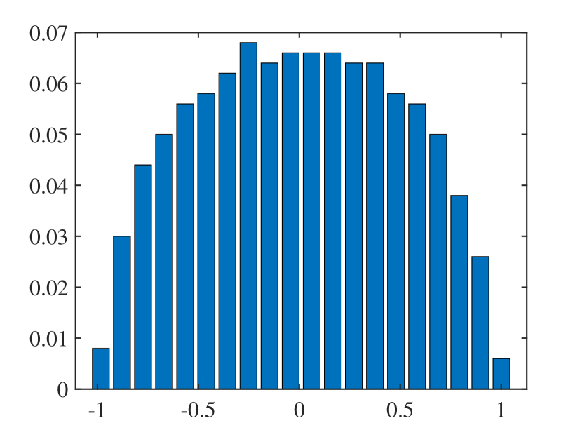
$N=500$

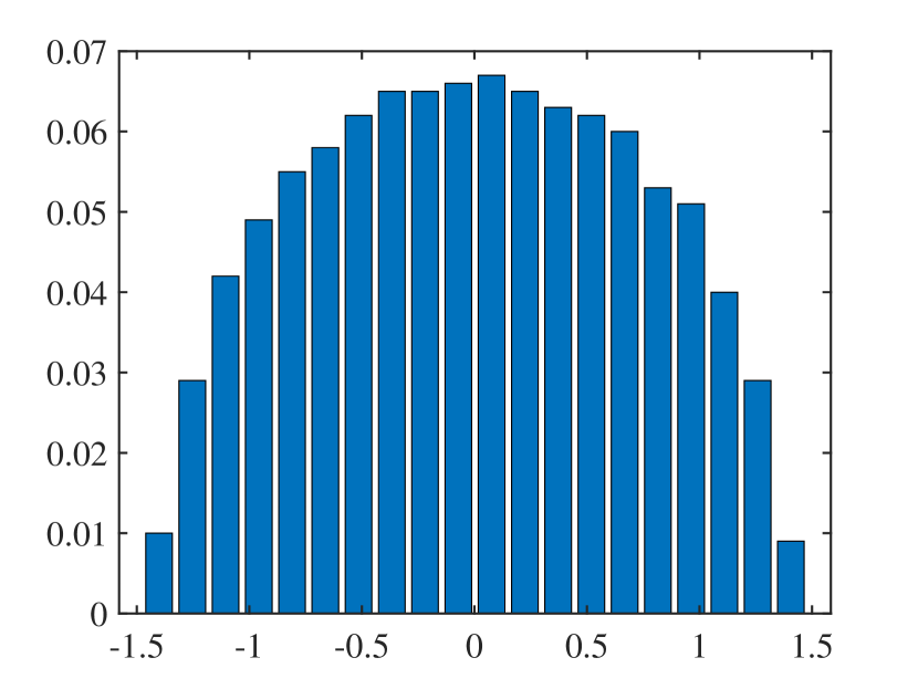
$N=1000$

Figure 1: The spectrum distribution of the numerical solution $\bar{U}_{P}^{(N)}$ of (4.1) generated by free BEM at $T=1$ for $\mu=-2,\sigma=1,$ and $h=2^{-10}$.

The unavailable exact solution is identified with a numerical approximation generated by the corresponding free STMs with a fine step size $h=2^{-14}$. The expectations are approximated by the Monte Carlo simulation with $M=250$ different free Brownian motion paths. Numerical approximations to (4.1) are generated by the free STMs with five different equidistant step sizes $2^{-11},2^{-10},2^{-9},2^{-8},2^{-7}$, i.e., $h_{R}=R\times h$ with $R=2^{3},2^{4},2^{5},2^{6},2^{7}$. The following 3 examples are handled similarly. See Figure 2 for the strong convergence order for $\mu=-2,\ \sigma=1.$ The order is close to $1$ since the noise is additive in (4.1); however, it does not conflict with the expected order $1/2$.

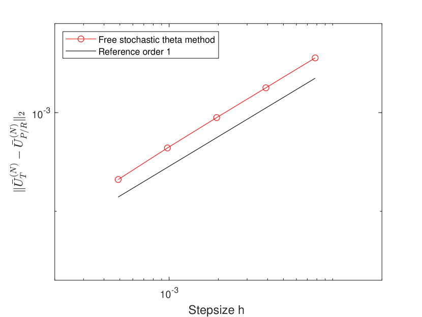
$\theta=0$

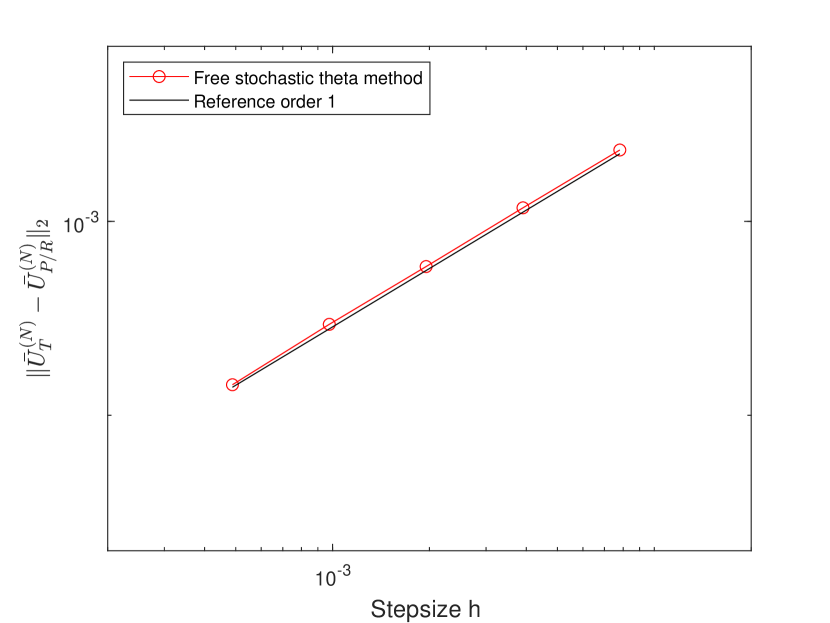
$\theta=0.5$

$\theta=1$

Figure 2: Strong convergence order simulations for the free STMs applied on (4.1).

Since the equation (4.1) does not have a trivial solution, we consider the exponential stability in mean square of the perturbation solution, i.e., the corresponding numerical sequence $\bar{U}^{(N)}_{P}$ and $\tilde{U}^{(N)}_{P}$ are generated by two different initial values ($\bar{U}^{(N)}_{0}=E$ and $\tilde{U}^{(N)}_{0}=2E$), where $E$ is the $N\times N$ identity matrix. The proof is similar to Subsection 3.3. Choosing $T=20$ and $N=100$ for $\mu=-4,\ \sigma=1$ will satisfy the assumptions in Theorem 6. Figure 3 demonstrates the free EM is not stable with large step size $h=1$, but free BEM is. On the premise of inheriting the exponential stability of the original equations, the free EM requires $16.11s$ with $h=1/4,$ while the free BEM only needs $1.05s$ with $h=4$. Thus, the free BEM is more efficient than the free EM. Figure 4 shows the exponential stability in mean square of the free BEM with different step sizes ($h=1/4,1/2,1,2,4$). It is clear that free BEM behaves stably for all given step sizes, which illustrates the exponential stability in mean square of the considered method.

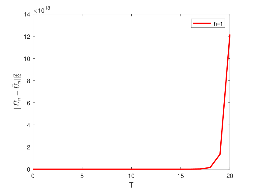
free EM

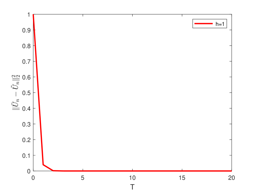
free BEM

Figure 3: The exponential stability in mean square of free EM and free BEM applied on (4.1) with $h=1$.

Figure 4: The exponential stability in mean square of free STM with $\theta=1$ applied on (4.1) with different step sizes.

4.2 Free Geometric Brownian Motion I

Consider the free Geometric Brownian Motion (free GBM) I

$${\rm d}U_{t}=\mu U_{t}{\rm dt}+\sqrt{U_{t}}{\rm d}W_{t}\sqrt{U_{t}},\ U_{0}={\bf 1},$$ (4.2)

where $\mu\in\mathbb{R}$ and ${\bf 1}$ is the unit operator in $\mathscr{F}$. We refer to [18] for the analytical solution. We note that the free GBM I doesn’t fulfill locally operator Lipschitz in the $L^{2}(\psi)$ norm; however, our numerical experiment still shows strong convergence. Figure 5 shows that the ability of free BEM to reproduce the spectrum distribution of the numerical solution $\bar{U}_{P}^{(N)}$. Since the density of the spectral distribution of $U_{t}$ is supported on the interval $[R_{1}(t),R_{2}(t)],$ where $R_{i}(t)=\frac{r_{i}(t)}{r_{i}(t)+1}e^{(\mu-1-r_{i}(t))t}$ and $r_{i}(t)=(-1\pm\sqrt{1+\frac{4}{t}})/2$ ($i=1,2$) [18], it has been observed from Figure 6 that the envolution of the supporting interval of the spectral distribution of $\bar{U}_{P}^{(N)}$ fits well with the theoretical values.

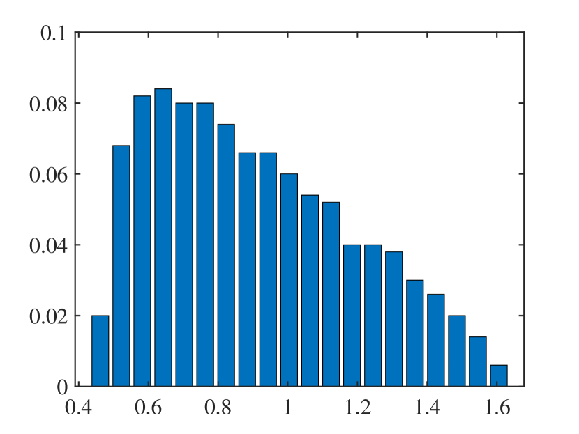
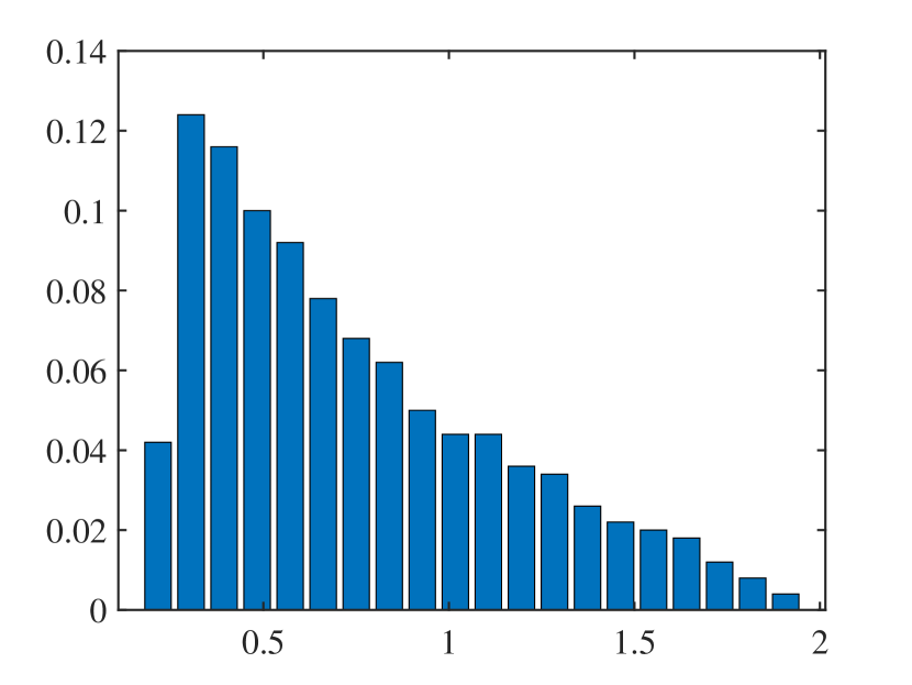
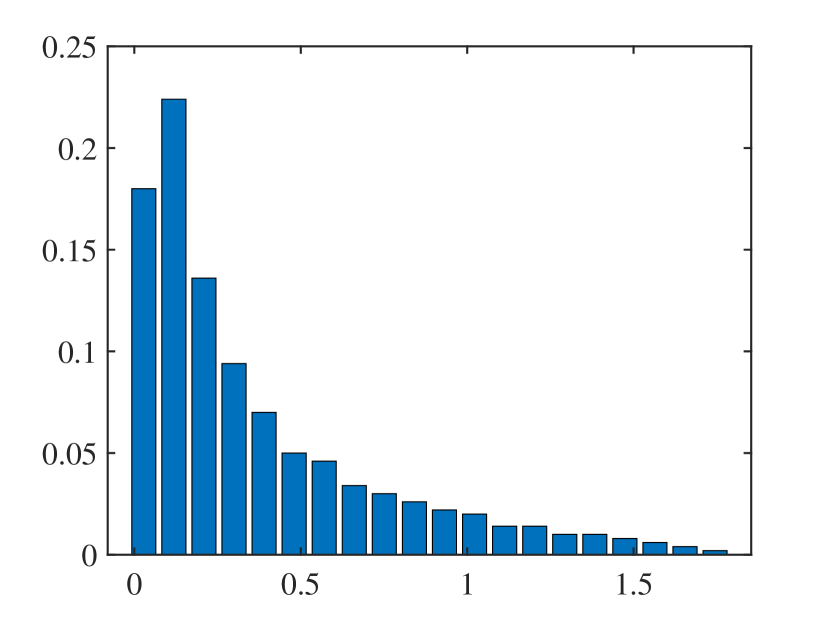
Figure 5: The spectrum distribution of the numerical solution $\bar{U}_{P}^{(N)}$ of (4.2) generated by free BEM at $T=100h$, $T=300h$, and $T=1024h$ with $\mu=-1$, $h=2^{-10},$ and $N=500$.

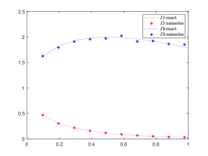
Figure 6: Comparison of boundaries of support interval $[I1=R_{1}(t),I2=R_{2}(t)]$ of the density of spectral distribution of (4.2).

Figure 7 shows that free STMs give errors that decrease proportionally to $h^{1/2}$, as shown in Theorem 2.

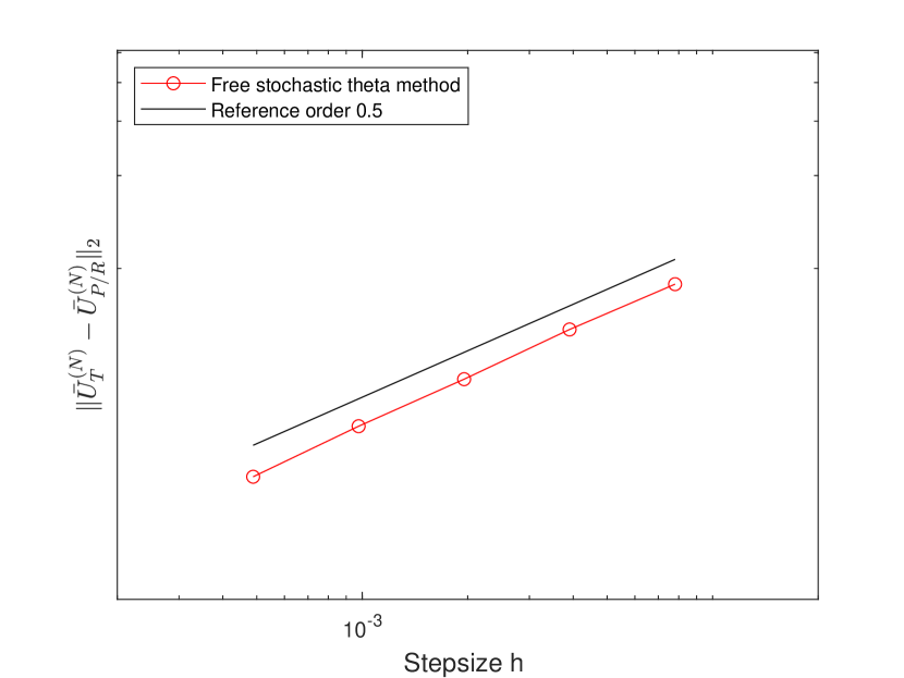
$\theta=0$

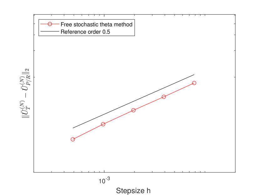
$\theta=0.5$

$\theta=1$

Figure 7: Strong convergence order simulations for the free STMs applied on (4.2).

To test the exponential stability in mean square of (4.2), we set $T=20,\ N=100$, and $\mu=-4,\ \sigma=1$ to satisfy the assumptions in Theorems 6. Figure 8 shows the free EM is not stable with large step size $h=1$, but free BEM is. Under the premise of inheriting the exponential stability in mean square of the original equations, the free EM requires $501.00s$ with $h=1/4,$ while the free BEM only requires $29.04s$ with $h=4$. Consequently, the free BEM is more efficient than the free EM. Figure 9 shows the exponential stability in mean square of the free BEM with different step sizes ($h=1/4,1/2,1,2,4$).

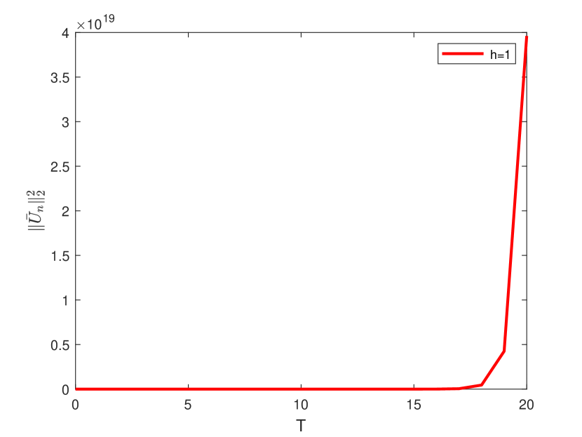
free EM

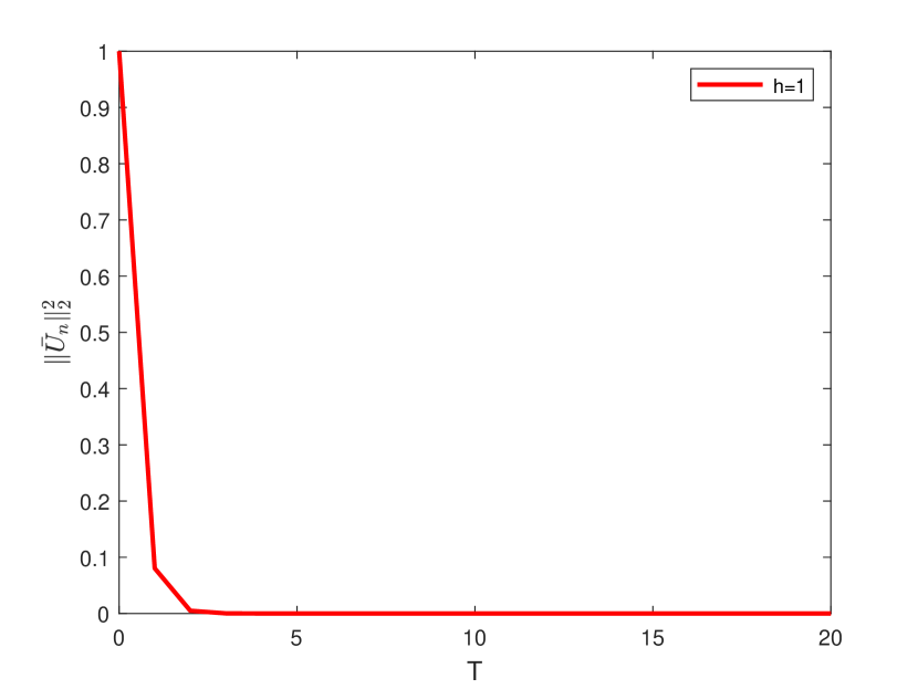
free BEM

Figure 8: The exponential stability in mean square of free EM and free BEM applied on (4.2) with $h=1$.

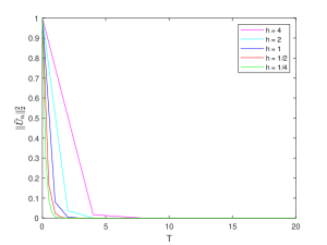
Figure 9: The exponential stability in mean square of free STM with $\theta=1$ applied on (4.2) with different step sizes.

4.3 Free Geometric Brownian Motion II

Consider the free Geometric Brownian Motion II

$${\rm d}U_{t}=\mu U_{t}{\rm dt}+U_{t}{\rm dW_{t}}+{\rm dW_{t}}U_{t},\ U_{0}={\bf 1},$$ (4.3)

where $\mu\in\mathbb{R}$. We refer to [18] for the analytical solution. See Figure 10 for the spectrum distribution of the numerical approximation (free BEM).

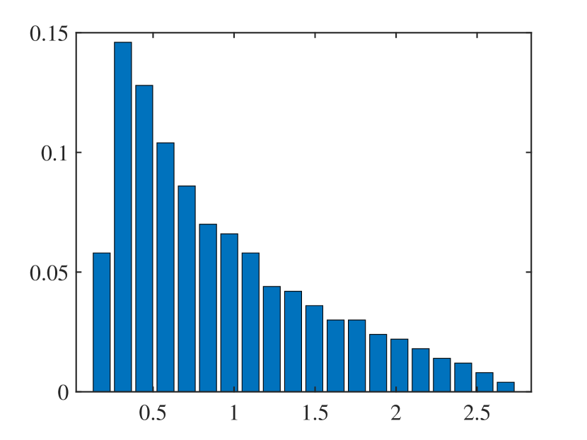
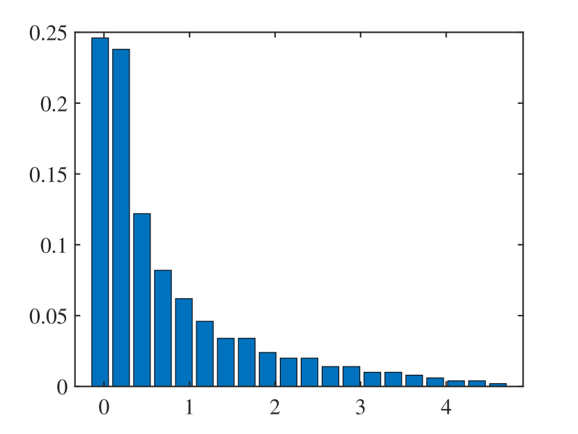
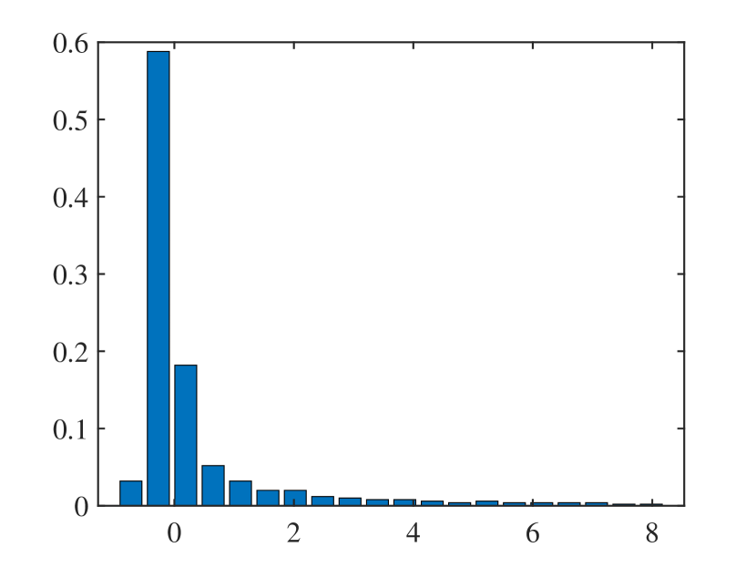
Figure 10: The spectrum distribution of the numerical solution $\bar{U}_{P}^{(N)}$ of (4.3) generated by free BEM at $T=100h$, $T=300h$, and $T=1024h$ with $\mu=-1$, $h=2^{-10},$ and $N=500$.

Figure 11 shows that free STMs give errors that decrease proportionally to $h^{1/2}$ as expected.

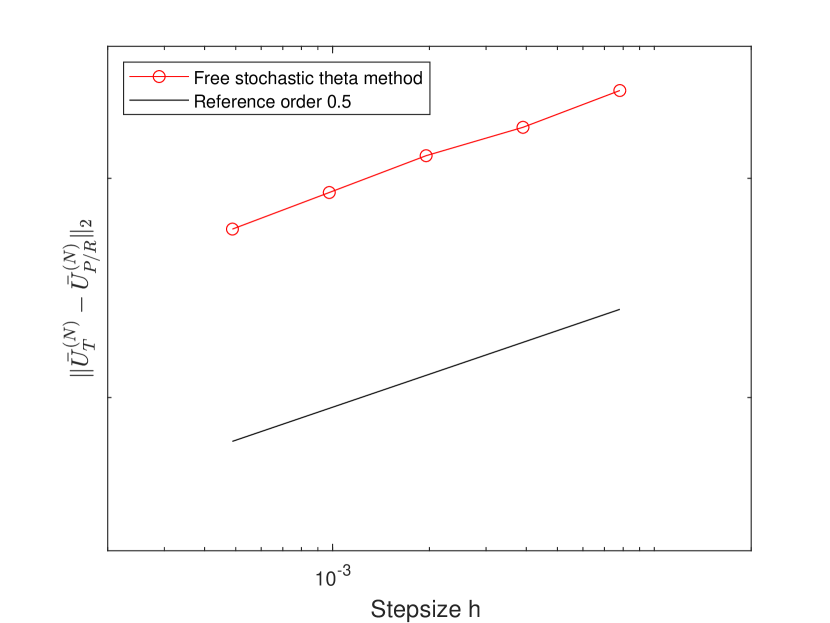
$\theta=0$

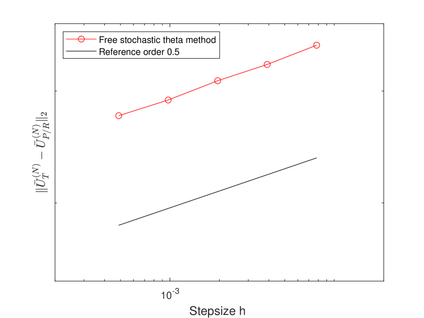
$\theta=0.5$

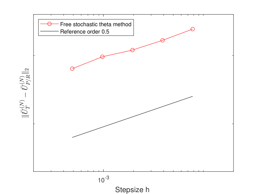
$\theta=1$

Figure 11: Strong convergence order simulations for the free STMs applied on (4.3).

To test the exponential stability in mean square of (4.3), we set $T=20,N=100,$ and $\mu=-4$ to satisfy the assumptions in Theorem 6. Figure 12 shows that the free EM is not stable with large step size $h=1$, but free BEM is. Moreover, on the premise of inheriting the exponential stability of original equations, the free EM requires $203.50s$ with $h=1/8,$ while the free BEM requires only $4.70s$ with $h=4$. Figure 13 indicates the exponential stability in mean square of the free BEM with different step sizes ($h=1/4,1/2,1,2,4$) .

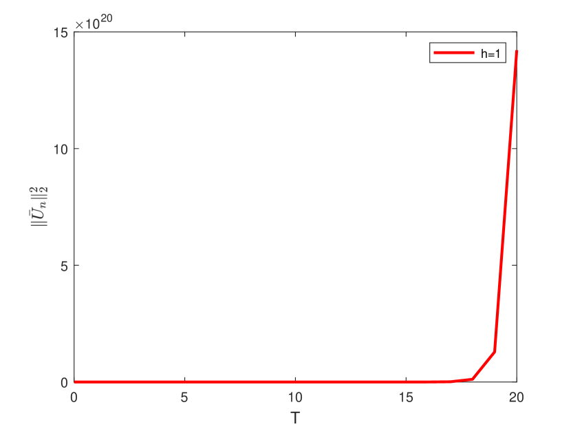
free EM

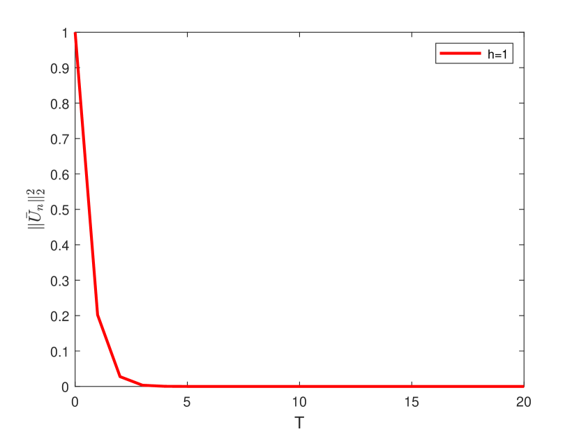
free BEM

Figure 12: The exponential stability in mean square of free EM and free BEM applied on (4.3) with $h=1$.

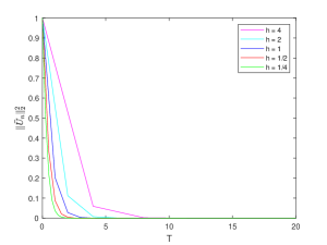
Figure 13: The exponential stability in mean square of free STM with $\theta=1$ applied on (4.3) with different step sizes.

4.4 Free CIR-process

Consider the Free CIR-process

$${\rm d}U_{t}=(\alpha-\beta U_{t}){\rm dt}+\frac{\sigma}{2}\sqrt{U_{t}}{\rm d}W_{t}+\frac{\sigma}{2}{\rm d}W_{t}\sqrt{U_{t}},\ U_{0}={\bf 1},$$ (4.4)

where $\alpha,\beta,\sigma\geq 0$ and satisfy the Feller condition $2\alpha\geq\sigma^{2}$. We note that the free CIR-process doesn’t fulfill locally operator Lipschitz in the $L^{2}(\psi)$ norm and Assumption 3; however, our numerical experiment still shows strong convergence and exponential stability in mean square. Figure 14 shows the spectrum distribution of the numerical solution $\bar{U}_{P}^{(N)}$ with $\theta=1$.

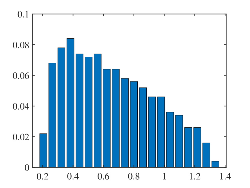
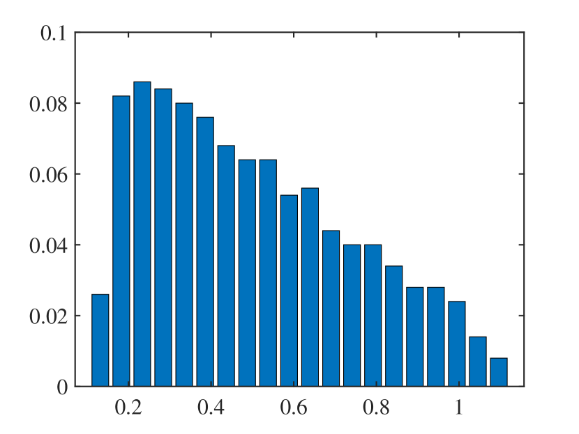
Figure 14: The spectrum distribution of the numerical solution $\bar{U}_{P}^{(N)}$ of (4.4) generated by free BEM at $T=300h$ and $T=4000h$ with $\alpha=2,\beta=4,\sigma=1$, $h=2^{-10},$ and $N=500$.

Figure 15 shows that the mean square errors decrease at a slope approaching 1/2 , which confirms the predicted convergence result.

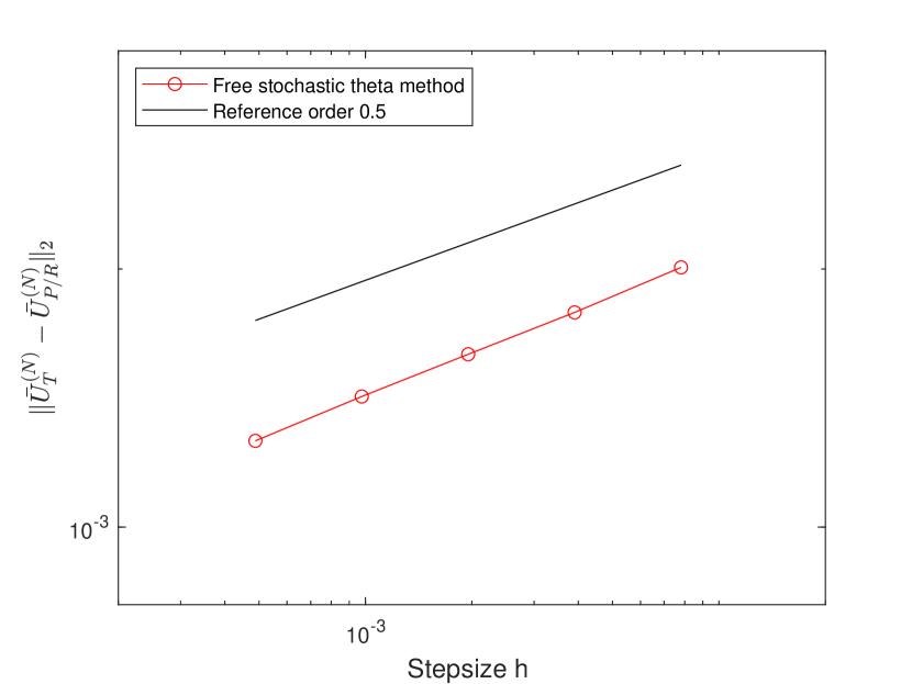
$\theta=0$

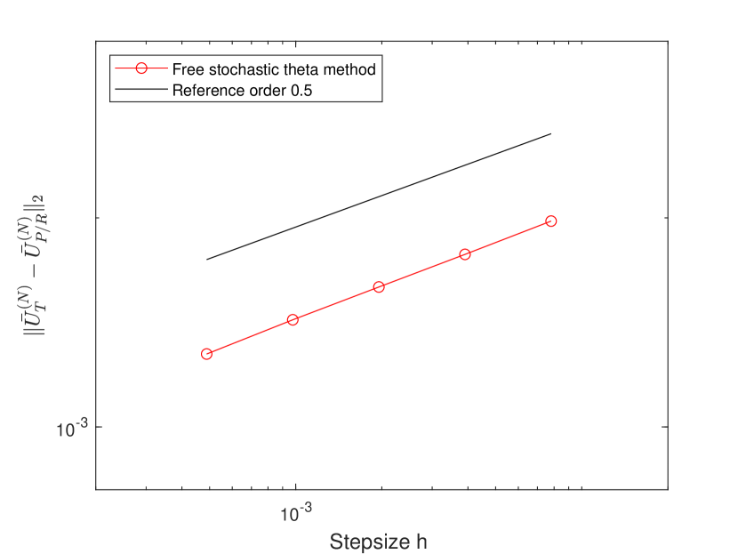
$\theta=0.5$

$\theta=1$

Figure 15: Strong convergence order simulations for the free STMs applied on (4.4).

Since the equation (4.4) does not have a trivial solution, we also consider the exponential stability in mean square of the perturbation solution as mentioned in Example 4.1, i.e., the corresponding numerical sequences $\bar{U}_{P}^{(N)}$ and $\tilde{U}_{P}^{(N)}$ are generated by two different initial values ( $\bar{U}^{(N)}_{0}=E$ and $\tilde{U}^{(N)}_{0}=2E$). Choosing $T=20$ and $N=100$ for $\alpha=2,\ \beta=4,\ \sigma=1$ to satisfy the assumptions in Theorem 6. Considering a large step size of $h=1$, Figure 16 demonstrates that the free EM is not stable, but the free BEM is. On the premise of inheriting the exponential stability of the original equations, the free EM requires $1162.32s$ with $h=1/4$, while the free BEM only needs $23.45s$ with $h=4$.

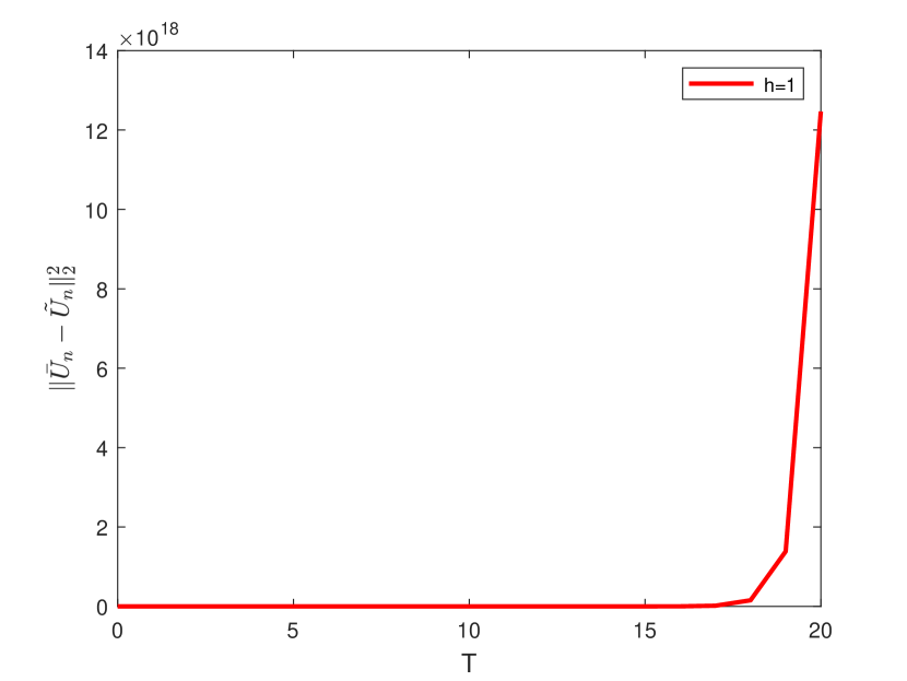
free EM

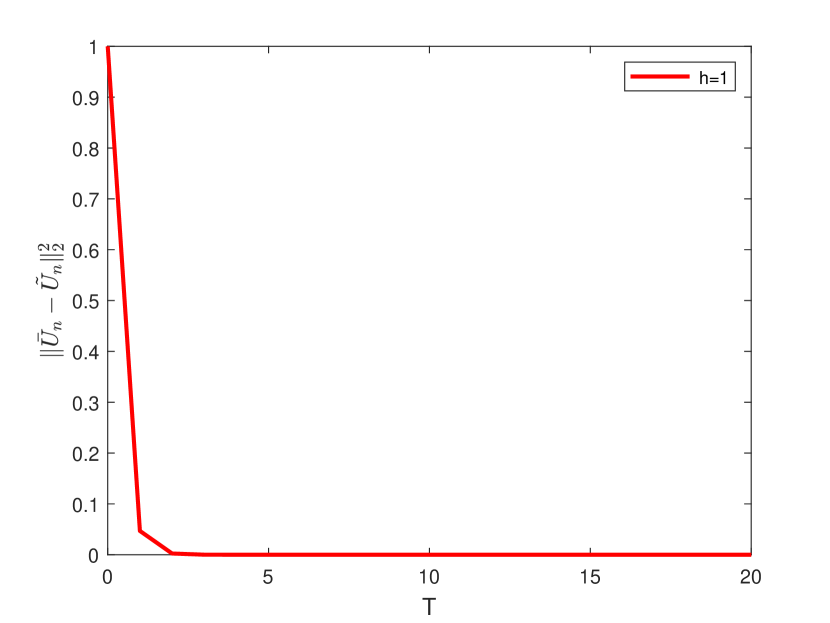
free BEM

Figure 16: The exponential stability in mean square of free EM and free BEM applied on (4.4) with $h=1$.

Figure 17 shows the exponential stability in mean square of the free BEM with different step sizes ($h=1/4,1/2,1,2,4$).

Figure 17: The exponential stability in mean square of free STM with $\theta=1$ applied on (4.4) with different step sizes.

5 Conclusions

In this work, we derived a family of free STMs with parameter $\theta\in[0,1]$ for numerically solving free SDEs. We recovered the standard convergence order $1/2$ of free STMs for free SDEs and derived conditions of exponential stability in mean square of the exact solution and the numerical solution. We obtained a step size restriction for the free STMs. It is shown that free STM with $\theta=1$ can inherit the exponential stability of the original equations for any given step size. Therefore, free STM with $\theta=1$ is superior to the free EM given previously in the literature. The theoretical analysis and numerical simulations demonstrated that the free STM with $\theta=1$ is very promising. It is shown that the numerical approximations generated by the free STMs to free SDEs with coefficients in the stochastic term that do not satisfy the locally operator Lipschitz condition also converge to the exact solution with order $1/2$ and behave exponentially stable. In addition, the solution to free SDEs should be self-adjoint, and the eigenvalues of the numerical solutions should be real. We obtained a few eigenvalues with a very small imaginary part when simulating free geometric Brownian motion I (4.2). Investigating the convergence and stability of free STMs applied to free SDEs with certain specific conditions on the coefficients $\alpha,\beta,\gamma$ and looking for numerical methods that are structure-preserving will be considered in future work.

References

- [1] A. Aleksandrov and V. Peller. Operator Lipschitz functions. arXiv:1611.01593, 2016.
- [2] M. Anshelevich. Itô formula for free stochastic integrals. Journal of Functional Analysis, 188(1):292–315, 2002.
- [3] W. J. Beyn and R. Kruse. Two-sided error estimates for the stochastic theta method. Discrete and Continuous Dynamical Systems-B, 14(2):389–407, 2010.
- [4] P. Biane and R. Speicher. Stochastic calculus with respect to free Brownian motion and analysis on Wigner space. Probability Theory and Related Fields, 112(3):373–409, 1998.
- [5] P. Biane and R. Speicher. Free diffusions, free entropy and free Fisher information. Annales de l’Institut Henri Poincare (B) Probability and Statistics, 37(5):581–606, 2001.
- [6] J. P. Bouchaud and M. Potters. Financial Applications of Random Matrix Theory: A Short Review, pages 823–850. Oxford University Press, 2015.
- [7] A. Bryden and D. J. Higham. On the boundedness of asymptotic stability regions for the stochastic theta method. BIT Numerical Mathematics, 43(1):1–6, 2003.
- [8] M. B. Giles. Multilevel Monte Carlo path simulation. Operations Research, 56(3):607–617, 2008.
- [9] H. Graf, H. Port, and G. Schlüchtermann. Free CIR processes. Infinite Dimensional Analysis, Quantum Probability and Related Topics, 25(03):2250012, 2022.
- [10] D. J. Higham. Mean-square and asymptotic stability of the stochastic theta method. SIAM Journal on Numerical Analysis, 38(3):753–769, 2000.
- [11] D. J. Higham. An algorithmic introduction to numerical simulation of stochastic differential equations. SIAM Review, 43(3):525–546, 2001.
- [12] D. J. Higham, X. Mao, and A. M. Stuart. Strong convergence of Euler-type methods for nonlinear stochastic differential equations. SIAM Journal on Numerical Analysis, 40(3):1041–1063, 2002.
- [13] D. J. Higham, X. Mao, and A. M. Stuart. Exponential mean-square stability of numerical solutions to stochastic differential equations. LMS Journal of Computation and Mathematics, 6:297–313, 2003.
- [14] D. J. Higham, X. Mao, and C. Yuan. Almost sure and moment exponential stability in the numerical simulation of stochastic differential equations. SIAM Journal on Numerical Analysis, 45(2):592–609, 2007.
- [15] C. W. Ho and P. Zhong. Brown measures of free circular and multiplicative Brownian motions with self-adjoint and unitary initial conditions. Journal of the European Mathematical Society, 25(6):2163–2227, 2022.
- [16] C. Huang. Exponential mean square stability of numerical methods for systems of stochastic differential equations. Journal of Computational and Applied Mathematics, 236(16):4016–4026, 2012.
- [17] M. Hutzenthaler, A. Jentzen, and P. E. Kloeden. Strong convergence of an explicit numerical method for SDEs with nonglobally Lipschitz continuous coefficients. The Annals of Applied Probability, 22(4):1611–1641, 2012.
- [18] V. Kargin. On free stochastic differential equations. Journal of Theoretical Probability, 24(3):821–848, 2011.
- [19] T. Kemp. The large-N limits of Brownian motions on . International Mathematics Research Notices, 2016(13):4012–4057, 2015.
- [20] P. E. Kloeden and E. Platen. Numerical Solution of Stochastic Differential Equations. Springer, Berlin, 1992.
- [21] B. Kümmerer and R. Speicher. Stochastic integration on the Cuntz algebra O∞. Journal of Functional Analysis, 103(2):372–408, 1992.
- [22] X. Mao. Stochastic differential equations and their applications. Horwood Publishing Series in Mathematics & Applications. Horwood Publishing Limited, Chichester, 1997.
- [23] G. N. Milstein and M. V. Tretyakov. Stochastic Numerics for Mathematical Physics. Springer Nature, Berlin, 2021.
- [24] J. A. Mingo and R. Speicher. Free Probability and Random Matrices, volume 35 of Fields Institute Monographs. Springer New York, New York, 2017.
- [25] A. Nica and R. Speicher. Lectures on the Combinatorics of Free Probability. London Mathematical Society Lecture Note Series. Cambridge University Press, 2006.
- [26] G. Pisier and Q. Xu. Non-commutative -spaces. Handbook of the geometry of Banach spaces. Elsevier, North-Holland, Amsterdam, 2003.
- [27] G. Schlüechtermann and M. Wibmer. Numerical solution of free stochastic differential equations. SIAM Journal on Numerical Analysis, 61(6):2623–2650, 2023.
- [28] R. Speicher. Free calculus. arXiv:0104004, 2001.
- [29] D. V. Voiculescu. Free probability theory: Random matrices and von neumann algebras. In S. D. Chatterji, editor, Proceedings of the International Congress of Mathematicians, pages 227–242, Basel, 1995. Birkhäuser Basel.
- [30] D. V. Voiculescu, N. Stammeier, and M. Weber, editors. Free probability and operator algebras. Münster Lectures in Mathematics. European Mathematical Society (EMS), Zürich, 2016. Lecture notes from the masterclass held in Münster, 2013.
- [31] X. Wang, J. Wu, and B. Dong. Mean-square convergence rates of stochastic theta methods for SDEs under a coupled monotonicity condition. BIT Numerical Mathematics, 60(3):759–790, 2020.