Robust projective measurements through measuring code-inspired observables

Abstract

Quantum measurements are ubiquitous in quantum information processing tasks, but errors can render their outputs unreliable. Here, we present a scheme that implements a robust projective measurement through measuring code-inspired observables. Namely, given a projective POVM, a classical code and a constraint on the number of measurement outcomes each observable can have, we construct commuting observables whose measurement is equivalent to the projective measurement in the noiseless setting. Moreover, we can correct $t$ errors on the classical outcomes of the observables’ measurement if the classical code corrects $t$ errors. Since our scheme does not require the encoding of quantum data onto a quantum error correction code, it can help construct robust measurements for near-term quantum algorithms that do not use quantum error correction. Moreover, our scheme works for any projective POVM, and hence can allow robust syndrome extraction procedures in non-stabilizer quantum error correction codes.

I Introduction

Quantum measurements, ubiquitous in quantum information processing tasks, are basic building blocks used in all quantum algorithms, such as in quantum sampling [1, 2, 3], quantum learning [4, 5, 6, 7, 8], quantum channel estimation [9, 10, 11, 12], quantum parameter estimation [13, 14, 15, 16, 17, 18, 19, 20], or universal quantum computations [21, 22, 23, 24]. However, errors in quantum measurements prevent these quantum algorithms from unlocking their full potential.

Quantum algorithms use either just the classical outputs of quantum measurements or both the classical outputs and the measured states. Near-term quantum algorithms such as quantum sampling, quantum learning, and quantum parameter estimation algorithms use primarily the classical outputs of quantum measurements. When errors afflict the classical outcomes these near-term quantum algorithms’ measurements, the precision of these quantum algorithms’ outputs suffers. Regarding near-term quantum algorithms, there has been a plethora of recent recent on the topic of quantum error mitigation [25, 26, 27, 28, 29, 30], where the goal is to reduce the statistical error of quantum measurements. This is achieved through repeated experiments and classical post-processing of the additional classical data obtained. However, the question of how to directly correct such measurement errors in these near-term algorithms without access to quantum error correction (QEC) is an open problem.

However, these mitigation schemes do not correct the measurement errors that occur. Hence arises the question that has been open since the dawn of the research field of quantum computing:

Universal quantum computations can use both quantum and classical outputs of measurements. Correction of both quantum and classical errors in measurements using stabilizer codes has been discussed in the context of data-syndrome codes [31, 32, 33, 34, 35, 36, 37], single-shot QEC [38, 39, 40], and fault-tolerant quantum computing [41]. However, the pertinent question of how to correct measurement errors for non-stabilizer codes, such as for bosonic codes [42, 43, 44, 45, 46], remains unanswered.

Here, we present a scheme that implements a robust projective measurement through measuring code-inspired observables. Namely, given a projective POVM, a classical code and a constraint on the number of measurement outcomes each observable can have, we construct commuting observables whose measurement is equivalent to the noiseless projective measurement. Moreover, we can correct $t$ errors on the classical outcomes of the observables’ measurement if the classical code corrects $t$ errors. The minimum number of commuting observables required depends on (1) the number of measurement outcomes for each commuting observable, (2) the number of measurement outcomes for the underlying projective measurement, and (3) the number of errors on classical outcomes that we wish to correct. We obtain bounds on the minimum number of commuting observables required based on bounds on the parameters of classical codes.

We suggest how to implement our scheme using ancillary coherent states. The requirements are modest. Namely, we need access to a linear coupling between the observables and ancillas, and the ability to perform homodyne measurement on the ancillas. Hence, using a modest amount of quantum control, we can in fact correct measurement errors, without need for quantum error correction codes.

We explain how our scheme allows the correction of measurement errors in any QEC code that satisfies the Knill-Laflamme QEC criterion [47]. Namely, given any QEC code that corrects a set of errors $\mathfrak{K}$, we bound the minimum number of commuting observables $n_{\mathfrak{K},t}$ required to correctly perform the syndrome extraction stage in the Knill-Laflamme recovery procedure if there are up to $t$ errors on the syndrome. Based on this, we give bounds on $n_{\mathfrak{K},t}$, and elucidate this bound for binary QEC codes and the binomial code.

We envision our scheme to complement existing quantum error mitigation techniques, and thereby enhance the performance of near-term quantum algorithms. In the longer term, our scheme can also enhance the design of fault-tolerant quantum computations on non-stabilizer codes, such as those reliant on bosonic codes [46, 48, 49].

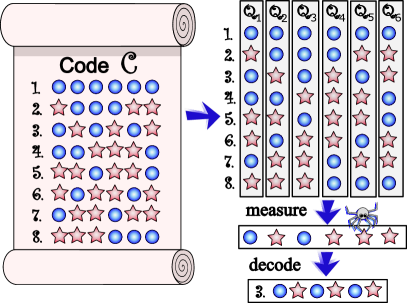
Figure 1: Our scheme. Suppose that a projective measurement $P$ projects a quantum state into one of 8 orthogonal subspaces. We label each subspace with a codeword of a classical code $C$. We depict a shortened Hamming code with 8 codewords. Each codeword is a 6-bit string, and the code corrects one error. Then we illustrate the commuting $q$-observables $Q_{1},\dots,Q_{6}$ as columns on the right side of the diagram. Each $q$-observable is an appropriate linear combination of projectors in $P$. Here, $q=2$, corresponding to binary outcome observables. A spider illustrates an error that occurs on the measurement outcome of $Q_{5}$. We can correct this error using the decoder of $C$, recovering the correct measurement outcome. We conclude that the quantum state has been projected to the third subspace.

II Measurements

We can describe a measurement as a POVM [50], which is a set of positive operators that sum to the identity operator. Without loss of generality, we can always focus on projective POVMs, where the positive operators are furthermore pairwise orthogonal projectors. This is because Naimark’s theorem ensures that for any POVM, we can always perform a projective POVM on an extended Hilbert space [51].

From the Born rule, measuring a projective POVM $P\coloneqq\{P_{1},\dots,P_{M}\}$ with pairwise orthogonal projectors on an input state $\rho$ yields the post-measurement state $\rho_{k}\coloneqq P_{k}\rho P_{k}/\operatorname{tr}[\rho P_{j}]$ with probability $p_{k}\coloneqq\operatorname{tr}[\rho P_{k}]$. We denote the measurement’s output as $(\rho_{k},k)$ where $k$ is the measurement’s classical outcome that allows us to uniquely identify the post-measurement state $\rho_{k}$.

Mathematically, an observable is a Hermitian operator. Consider an observable $O=\sum_{k}\lambda_{k}P_{k}$, where $\lambda_{k}$ are distinct real numbers for different values of $k$. Measurement of $O$ on $\rho$ gives an output $(\rho_{k},\lambda_{k})$ comprising of a post-measurement state and some eigenvalue of $O$. According to the Born rule, we obtain $(\rho_{k},\lambda_{k})$ with probability $p_{k}$. Since there exists a function that maps $\lambda_{k}$ back to $k$, the measurement of $O$ is the same as the measurement of $P$.

Errors affect a measurement’s output in two different ways. First, errors can corrupt the classical outcome $k$. Such errors can lead us to mistakenly conclude that the post-measurement state is $\rho_{v}$ for $v\neq k$ when the true post-measurement state is in fact $\rho_{k}$. Second, errors can corrupt the post-measurement state $\rho_{k}$. Here, we propose a measurement scheme that allows correction of errors on classical outcomes.

Now, let $q$ be an integer where $q\geq 2$, and let us define a Hermitian operator with $q$ distinct eigenvalues as a $q$-observable. Operationally, the integer $q$ counts the number of possible measurement outcomes of each observable.

III Commuting observables from classical codes

In the observable $O$, the integers $1,\dots,M$ label $M$ distinct measurement outcomes. Consider a classical code $C$ comprising of $M$ distinct codewords. When $C$ is a $q$-ary code of length $n$, each codeword is a vector in $\{0,1,\dots,q-1\}^{n}$. We denote

$${\bf x}^{(k)}=(x^{(k)}_{1},\dots,x^{(k)}_{n})$$

as the $k$th codeword of $C$, and we can write $C=\{{\bf x}^{(k)}:k=1,\dots,M\}$.

Each integer $1,\dots,M$ labels exactly one codeword in $C$. The encoder $E_{C}$ of $C$ is a bijective map from the classical labels in $\{1,\dots,M\}$ to codewords in $C$. Namely, $E_{C}(k)={\bf x}^{(k)}$. Without errors on the components of ${\bf x}^{(k)}$, a decoder of $C$ performs the inverse map of $E_{C}$, and maps the codeword ${\bf x}^{(k)}$ back to the label $k$.

In the measurement of $P$, errors could afflict its classical outcome. To address this, we propose the measurement of $n$ commuting $q$-observables $Q_{1},\dots,Q_{n}$ that encode redundant information about $P$. We denote the classical outcome of $Q_{j}$’s measurement as $y_{j}$ and denote the output of the measurements of $Q_{1},\dots,Q_{n}$ as $(\tau,{\bf y})$ where $\tau$ denotes the post-measurement state and ${\bf y}=(y_{1},\dots,y_{n})$. We want the $q$-observables to be consistent with $P$, in the sense that measurement of the $q$-observables performs the same measurement as $P$ in the noiseless setting. Hence we give the following definition.

Definition 1.

Let $P$ be a projective POVM and $Q_{1},\dots,Q_{n}$ be commuting observables. The observables $Q_{1},\dots,Q_{n}$ are consistent with $P$ if there exists a function $f$ such that for any output $(\tau,{\bf y})$ of the measurement of $Q_{1},\dots,Q_{n}$ on $\rho$, we have $\tau=\rho_{f({\bf y})}$.

We propose to construct $q$-observables using information about a projective POVM $P$ and a classical $q$-ary code $C$. Namely, for $j=1,\dots,n$ we define the $q$-observables as

$$Q_{j}(C,P)\coloneqq\sum_{k=1}^{M}x^{(k)}_{j}P_{k}.$$ (1)

When the context is clear, we use $Q_{j}$ to denote $Q_{j}(C,P)$. From the orthogonality of the projectors $P_{k}$, the observables $Q_{1},\dots,Q_{n}$ are pairwise commuting, which allows us to measure $Q_{1},\dots,Q_{n}$ in any order.

In our construction, the correctibility of errors on the measurement outcomes of our $q$-observables depends on the minimum distance of $C$, given by

$$d(C)\coloneqq\min_{{\bf y}\neq{\bf z}\in C}d_{H}({\bf y},{\bf z}),$$

where $d_{H}({\bf y},{\bf z})\coloneqq|\{i:y_{i}\neq z_{i}\}|$ is the Hamming distance between tuples ${\bf y}$ and ${\bf z}$. Namely, we can correct any $t(C)\coloneqq\lfloor(d(C)-1)/2\rfloor$ errors on the classical outcomes of $Q_{1},\dots,Q_{n}$.

A decoder of a classical code can correct up to $t(C)$ measurement errors on ${\bf y}$. This is because a noiseless ${\bf y}$ must be a codeword in $C$. Here, a decoder $\mathcal{D}$ of a code $C$ is a function $\mathcal{D}:\{0,\dots,q-1\}^{n}\to\{1,\dots,M\}$ which maps an $n$-tuple to an index that labels the codewords. Given some non-negative integer $a$, we say that $\mathcal{D}$ is an $a$-decoder of $C$, if for all $k=1,\dots,M,$ and for all ${\bf y}$ such that $d({\bf y},{\bf x}_{k})\leq a$, we have

$$\mathcal{D}({\bf y})=k.$$ (2)

An $a$-decoder corrects $a$ errors. When $d(C)=d$, then there is a $t(C)$-decoder for $C$. Our main result is the following.

Theorem 1.

Let $C$ be a $q$-ary code of length $n$, and let $\mathcal{D}$ be a $t(C)$-decoder for $C$. We measure $Q_{1}(C,P),\dots,Q_{n}(C,P)$ on a quantum state $\rho$, and obtain the classical outcome ${\bf y}=(y_{1},\dots,y_{n})$ along with the post-measurement state $\tau$. Suppose that at most $t(C)$ components of ${\bf y}$ have been corrupted. Then $\tau=\rho_{\mathcal{D}({\bf y})}$.

Proof.

Let ${\bf z}=(z_{1},\dots,z_{n})$ denote the classical outcome if no errors occurred. Then, ${\bf z}-{\bf y}$ has a Hamming weight of at most $t$. Furthermore, we have

$$\mathcal{D}({\bf z})=\mathcal{D}({\bf y}).$$ (3)

Case 1: No errors on measurement outcomes. When we measure the observable $Q_{j}(C,P)$ and obtain the classical outcome $z_{j}$, the resultant state must be on the support of the projector

$$P_{j,z_{j}}=\sum_{k:z_{j}=x_{k,j}}P_{k}.$$ (4)

After measuring the observables $Q_{1}(C,P),\dots,Q_{n}(C,P)$, we obtain the classical outcomes $z_{1},\dots,z_{n}$. Then the state $\tau$ is on the support of

$$\prod_{j=1}^{n}P_{j,z_{j}}=\sum_{k:z_{j}=x_{k,j},j=1,\dots,n}P_{k}=\sum_{k:{\bf z}={\bf x}_{k}}P_{k}.$$ (5)

From (5), ${\bf z}$ must belong to $C$. Since there are no repeated codewords in $C$, there is a unique $k$ for which ${\bf z}={\bf x}_{k}$. Together with the fact that $t(C)\geq 0$, it follows that

$$\prod_{j=1}^{n}P_{j,z_{j}}=P_{\mathcal{D}({\bf z})}.$$ (6)

The state $\tau$ must be on the support of $P_{\mathcal{D}({\bf z})}$, which means that $\tau=\rho_{\mathcal{D}({\bf z})}$.

Case 2: At most $t(C)$ errors on classical outcomes. From case 1, we know that $\tau=\rho_{\mathcal{D}({\bf z})}$. Since $\mathcal{D}({\bf y})=\mathcal{D}({\bf z})$, we have $\tau=\rho_{\mathcal{D}({\bf y})}$. ∎

In our proof of Theorem 1, we show that in the noiseless setting, the $n$-tuple of classical outcomes is a codeword of $C$. When there are at most $t(C)$ errors on the classical outcomes, the decoder $\mathcal{D}$ corrects these errors. Hence, the observables $Q_{1}(C,P),\dots,Q_{n}(C,P)$ are consistent with $P$, even in the presence of some errors on the classical outcomes.

As an example, consider a scheme that uses the shortened Hamming code $C_{6}$ and a projective POVM $P=\{P_{1},\dots,P_{8}\}$ to define the six binary observables to measure both in the noiseless setting. In this example, the parameters of the code are $q=2,n=6,d(C_{6})=3,$ and $M=8.$ Now the code $C_{6}$ is a linear code generated by binary vectors $a_{1}=\texttt{100011}$, $a_{2}=\texttt{010101},$ and $a_{3}=\texttt{001110}$, and has eight codewords given by

$${\bf x}_{1} =\texttt{000000},$$

$${\bf x}_{2} =\texttt{100011}=a_{1},$$

$${\bf x}_{3} =\texttt{010101}=a_{2},$$

$${\bf x}_{4} =\texttt{001110}=a_{3},$$

$${\bf x}_{5} =\texttt{110110}=a_{1}+a_{2},$$

$${\bf x}_{6} =\texttt{101101}=a_{1}+a_{3},$$

$${\bf x}_{7} =\texttt{011011}=a_{2}+a_{3},$$

$${\bf x}_{8} =\texttt{111000}=a_{1}+a_{2}+a_{3}.$$ (7)

Applying the definition (1) along with the form for the codewords in (7), the corresponding binary observables are

$$Q_{1}(C_{6},P) =P_{2}+P_{5}+P_{6}+P_{8}$$

$$Q_{2}(C_{6},P) =P_{3}+P_{5}+P_{7}+P_{8}$$

$$Q_{3}(C_{6},P) =P_{4}+P_{6}+P_{7}+P_{8}$$

$$Q_{4}(C_{6},P) =P_{3}+P_{4}+P_{5}+P_{6}$$

$$Q_{5}(C_{6},P) =P_{2}+P_{4}+P_{5}+P_{7}$$

$$Q_{6}(C_{6},P) =P_{2}+P_{3}+P_{6}+P_{7}.$$

We illustrate these binary observables in Figure 1. Now consider no errors on classical outcomes. When we measure $Q_{1}(C_{6},P)$ and obtain the classical outcome 0, the state must be on the support of $I-Q_{1}(C_{6},P)=P_{1}+P_{3}+P_{4}+P_{7}$, where $I$ denotes the identity operator. If we measure $Q_{2}(C_{6},P)$ and obtain the classical outcome 1, then the state is on the support of $P_{1}+P_{3}+P_{4}+P_{7}$ and $P_{3}+P_{5}+P_{7}+P_{8}$. Hence the state is on the support of $P_{3}+P_{7}$. If we measure $Q_{3}(C_{6},P)$ and obtain the classical outcome 1, then the state is on the support of $P_{3}+P_{7}$ and $P_{4}+P_{6}+P_{7}+P_{8}$. Hence the state is on the support of $P_{7}$. Further measurements of the observables $Q_{4}(C_{6},P),Q_{5}(C_{6},P),Q_{6}(C_{6},P)$ give redundant information about where the state is projected on, and we obtain the codeword ${\bf x}_{7}$ as the classical outcome.

In Figure 1 we illustrate the measurement of the binary observables $Q_{1}(C_{6},P),\dots,Q_{n}(C_{6},P)$ when an error afflicts the classical outcome of $Q_{5}(C_{6},P)$.

IV Implications

Combinatorics:- What is the minimum number of $q$-observables required to correct $t$ errors on the classical outcome of a projective POVM with $M$ projectors? We answer this question in the following.

Corollary 2.

Let $P$ be a projective POVM with $M$ projectors. Let $n_{q}(M,d)$ to be the shortest $n$ such that there exists a code of length $n$ and with at least $M$ codewords and distance at least $d$. Let $n_{q,t,M}$ be the smallest integer such that there exist observables $Q_{1},\dots,Q_{n}$ consistent with $P$, even after any $t$ errors occur on the classical outcomes of $Q_{1},\dots,Q_{n}$. Then $n_{q,t,M}=n_{q}(M,2t+1)$.

Proof.

From Theorem 1, we know that the condition for $Q_{1},\dots,Q_{n}$ to be consistent with $P$ after $t$ errors occur on the classical outcomes is equivalent to the condition that a $q$-ary classical code $C$ has length $n$, distance at least $2t+1$, and has $M$ codewords. ∎

The combinatorics of $n_{q}(M,d)$ directly relates to the combinatorics of $A_{q}(n,d)$, where $A_{q}(n,d)$ is the maximum number of codewords in a $q$-ary code with Hamming distance $d$ and with codewords having $n$ components. Note that $n_{q,t,q}=2t+1$ through the use of a $q$-ary repetition code. Using results on the combinatorics of $A_{q}(n,d)$ and $n_{q}(M,d)$ [52], we illustrate the values of $n_{q,t,M}$, in Table 1 for $q=2$, $t=1,2,3$ and $2\leq M\leq 40$.

$t\backslash M$	2	4	6	8	12	16	20	38-40
1	3	$6$	$7$	$7$	$8$	$8$	$9$	10
2	5	$9$	$10$	$11$	$11$	$12$	$12$	14
3	7	$12$	$14$	$14$	$15$	$15$	$16$	18

Table 1: Some values of $n_{2,t,M}$.

When the number $M$ of projectors in $P$ is very large, we can bound $M$ in terms of the volume of a $q$-ary Hamming ball of radius $t$, which we denote as $V_{q,n}(t)\coloneqq\sum_{j=0}^{t}\binom{n}{j}(q-1)^{j}$. Namely,

$$q^{n}/V_{q,n}(2t)\leq M\leq q^{n}/V_{q,n}(t),$$ (8)

where the upper and lower bounds are the Hamming bound and Gilbert-Varshamov bound respectively [53]. bounds such as Johnson’s bound [54] or linear programming bounds for classical codes [55, 56] can tighten the upper bound in (8). For large $n$ and $t<n(q-1)/q$, we have $\frac{1}{n}\log_{q}V_{q,n}(t)=H_{q}(t/n)+o(1)$, where $H_{q}(x)\coloneqq-x\log_{q}x-(1-x)\log_{q}(1-x)+x\log_{q}(q-1)$ denotes the $q$-ary entropy function. Given $\tau$ as the fraction of errors on the classical outcomes of the measurement of our $q$-observables, for large $M$, we have

$$\frac{\log_{q}M}{1-H_{q}(\tau)+o(1)}\leq n_{q,\tau n,M}\leq\frac{\log_{q}M}{1-H_{q}(2\tau)+o(1)}.$$ (9)

Implementation:- Similarly to Refs. [57, 58], we can couple our quantum state to $n$ bosonic modes initialized as coherent states $|\alpha_{1}\rangle,\dots,|\alpha_{n}\rangle$ and measure the modes to implement our scheme. Let $\hat{n}_{j}$ be the number operator on the $j$th mode, and suppose that $2\pi|\alpha_{j}|^{2}\gg q$. The interaction Hamiltonians

$$W_{j}=\gamma Q_{j}\otimes\hat{n}_{j}$$ (10)

model a dispersive coupling between the quantum system and the ancillary bosonic modes.

Now let $|\phi\rangle$ be a state for which $Q_{j}|\phi\rangle=z_{j}|\phi\rangle$ for all $j=1,\dots,n$. Then $W_{j}|\phi\rangle|\alpha_{j}\rangle=|\phi\rangle(\gamma z_{j}\hat{n}_{j}|\alpha_{j}\rangle)$. Hence $e^{-iW\theta}|\phi\rangle|\alpha_{j}\rangle=|\phi\rangle e^{-i\theta\gamma z_{j}\hat{n}_{j}}|\alpha_{j}\rangle=|\phi\rangle|e^{-i\theta\gamma z_{j}}\alpha_{j}\rangle$. With $\theta=2\pi/(q\gamma)$, the initial phase space distribution of the $j$th mode with radius $|\alpha_{j}|^{2}$ and standard deviation $1/\sqrt{2}$ maps to up to $q$ different equiangular rotations in the complex plane. Using balanced homodyne detection [59] we can measure the quadratures of the output bosonic fields. Because we chose $2\pi|\alpha_{j}|^{2}\gg q$, the distributions for different $z_{j}$ will be distinguishable. Hence we project onto the eigenspaces of $Q_{j}$ in a non-destructive way. Repeating the procedure for $j=1,\dots,n$ allows us to obtain the classical outcome $(z_{1},\dots,z_{n})$ in the noiseless setting. From Theorem 1, we can correct up to $t$ errors on $(z_{1},\dots,z_{n})$ using a classical decoder.

Application (Quantum error correction):- We can describe the recovery channel of any QEC code as a two-stage process [47]. In the first stage, we measure a carefully chosen projective measurement with POVM $\Pi^{\prime}$. Upon measuring $\Pi^{\prime}$, we get a classical outcome and a quantum output. The classical output labels the subspace that the quantum output resides in. In the second stage, a unitary operation dependent on the classical outcome brings the quantum output back to the codespace.

The projectors in $\Pi^{\prime}$ depend on the QEC code and the set of operators $\mathfrak{K}$ to be corrected. Since the number of correctible spaces of the code is at most $|\mathfrak{K}|$, and at most one projector corresponds to an uncorrectible space, we have $|\Pi^{\prime}|\leq|\mathfrak{K}|+1$. For a distance $p$-ary QEC code on $m$ qudits that corrects $k$ errors, we can choose $\mathfrak{K}$ so that $|\mathfrak{K}|=V_{p^{2},m}(k)$. From [47], $|\Pi^{\prime}|\leq|\mathfrak{K}|$. Hence, for an $m$ qubit QEC code that corrects a single error (has distance 3), we have $|\Pi^{\prime}|\leq 2+3m$.

As an example, consider the optimal non-additive nine-qubit binary QEC code that has codespace of dimension 12, and with distance 3 [60]. In this case $|\Pi^{\prime}|\leq 29$ From Table 1, deploying our scheme with 10 binary observables allows the correction of up to one error on the classical outcome of $\Pi^{\prime}$. In contrast, the noiseless decoding of this non-additive nine-qubit code in Ref. [60] requires five binary observables, and repeating these measurements thrice to allow the correction of one error necessitates the use of 15 binary observables, which is greater than the 10 binary observables our scheme requires.

Now consider $p$-ary QEC codes that correct $k$ errors using $m$ qudits. Setting $\tau$ as the maximum fraction of errors on the classical outcome of $\Pi^{\prime}$, from (9), the minimum number $n$ of binary observables required to allow robust syndrome extraction according to $\Pi^{\prime}$ satisfies the bounds

$$n \geq\frac{m(H_{p^{2}}(k/m)\log_{2}p)+o(1))}{\log_{2}H_{q}(\tau)+o(1)}$$ (11)

$$n \leq\frac{m(H_{p^{2}}(2k/m)\log_{2}p)+o(1))}{\log_{2}H_{q}(2\tau)+o(1)}.$$ (12)

As another example, we consider the binomial code [44], which is a bosonic code on a single mode that corrects gain errors, loss errors and phase errors. Here, loss errors, gain errors and phase errors are monomials of $a$, $a^{\dagger}$ and $a^{\dagger}a$ respectively where $a$ denotes the mode’s lowering operator. Namely, a binomial code that corrects $g_{1}$ gain errors, $g_{0}$ loss errors, and $k$ phase errors has as its set of correctible errors $\mathfrak{K}=\{a^{j}:j=0,\dots,g_{0}\}\cup\{(a^{\dagger})^{j}:j=0,\dots,g_{1}\}\cup\{(a^{\dagger}a)^{j}:j=0,\dots,k\}.$ Clearly, $|\mathfrak{K}|=g_{0}+g_{1}+k+1$. Such a binomial code has two parameters, the gap $g=g_{0}+g_{1}+1$, and $N=\max\{g0,g1,2k\}$ and encodes one logical qubit, and is defined by the logical codewords in [44, Eq. (7)]. For such a binomial code where $g_{0}=g_{1}=k$, we have $|\Pi^{\prime}|\leq 3k+2$. In Table 2, we present the minimum number of binary observables that are consistent with $\Pi^{\prime}$ after the occurrence of up to a single error on the classical outcome of their measurement.

$k$	1	2	3	4	5	6	7	8
$|\Pi^{\prime}|$	5	$8$	$11$	$14$	$17$	$20$	$23$	26
$n$	7	$7$	$8$	$8$	$9$	$9$	$10$	10

Table 2: Some values of the minimum number of binary observables consistent with $\Pi^{\prime}$ needed to correct up to one error on the classical outcomes of their measurement $n$, and furthermore correct $k$ gain, loss and phase errors.

V Discussions

We proposed a set of commuting $q$-observables whose measurement is consistent with a given projective measurement, even after some errors corrupt the classical outcomes of the measurement of the observables. Hence, measuring these commuting observables effectively implements a robust projective measurement.

There is potential to study how near-term quantum algorithms that do not rely on QEC can be improved using our scheme in realistic settings. Moreover, it would be interesting to explore the implementation of our scheme with other non-stabilizer codes, such as concatenated cat codes [42, 61], rotation-invariant codes [46], permutation-invariant codes [62, 63, 64, 65, 45, 66, 67], codeword-stabilized codes [68], error-avoiding codes [69, 70, 71], and certain codes that lie within the ground space of local Hamiltonians [72].

VI Acknowledgements

YO acknowledges support from EPSRC (Grant No. EP/W028115/1).

References

- Tillmann et al. [2013] M. Tillmann, B. Dakić, R. Heilmann, S. Nolte, A. Szameit, and P. Walther, Experimental boson sampling, Nature photonics 7, 540 (2013).
- Lund et al. [2017] A. P. Lund, M. J. Bremner, and T. C. Ralph, Quantum sampling problems, bosonsampling and quantum supremacy, npj Quantum Information 3, 15 (2017).
- Wild et al. [2021] D. S. Wild, D. Sels, H. Pichler, C. Zanoci, and M. D. Lukin, Quantum sampling algorithms for near-term devices, Physical Review Letters 127, 100504 (2021).
- Bisio et al. [2010] A. Bisio, G. Chiribella, G. M. D’Ariano, S. Facchini, and P. Perinotti, Optimal quantum learning of a unitary transformation, Phys. Rev. A 81, 032324 (2010).
- Arunachalam and de Wolf [2017] S. Arunachalam and R. de Wolf, Guest column: A survey of quantum learning theory, ACM Sigact News 48, 41 (2017).
- Haah et al. [2017] J. Haah, A. W. Harrow, Z. Ji, X. Wu, and N. Yu, Sample-optimal tomography of quantum states, IEEE Transactions on Information Theory 63, 5628 (2017).
- Lai and Cheng [2022] C.-Y. Lai and H.-C. Cheng, Learning quantum circuits of some t gates, IEEE Transactions on Information Theory 68, 3951 (2022).
- Ouyang and Tomamichel [2022] Y. Ouyang and M. Tomamichel, Learning quantum graph states with product measurements, in 2022 IEEE International Symposium on Information Theory (ISIT) (2022) pp. 2963–2968.
- Escher et al. [2011] B. Escher, R. L. de Matos Filho, and L. Davidovich, General framework for estimating the ultimate precision limit in noisy quantum-enhanced metrology, Nature Physics 7, 406 (2011).
- Hayashi [2011] M. Hayashi, Comparison between the Cramer-Rao and the mini-max approaches in quantum channel estimation, Commun. Math. Phys. 304, 689 (2011).
- Pirandola et al. [2019] S. Pirandola, R. Laurenza, C. Lupo, and J. L. Pereira, Fundamental limits to quantum channel discrimination, npj Quantum Information 5, 50 (2019).
- Zhou and Jiang [2021] S. Zhou and L. Jiang, Asymptotic theory of quantum channel estimation, PRX Quantum 2, 010343 (2021).
- Helstrom [1967] C. Helstrom, Minimum mean-squared error of estimates in quantum statistics, Physics Letters A 25, 101 (1967).
- Helstrom [1976] C. W. Helstrom, Quantum detection and estimation theory (Academic press, 1976).
- Holevo [2011] A. S. Holevo, Probabilistic and statistical aspects of quantum theory (Edizioni della Normale, 2011).
- Hayashi and Matsumoto [2008] M. Hayashi and K. Matsumoto, Asymptotic performance of optimal state estimation in qubit system, Journal of Mathematical Physics 49, 102101 (2008).
- Albarelli et al. [2019] F. Albarelli, J. F. Friel, and A. Datta, Evaluating the Holevo Cramér-Rao bound for multiparameter quantum metrology, Phys. Rev. Lett. 123, 200503 (2019).
- Sidhu et al. [2021] J. S. Sidhu, Y. Ouyang, E. T. Campbell, and P. Kok, Tight bounds on the simultaneous estimation of incompatible parameters, Phys. Rev. X 11, 011028 (2021).
- Conlon et al. [2021] L. O. Conlon, J. Suzuki, P. K. Lam, and S. M. Assad, Efficient computation of the Nagaoka–Hayashi bound for multiparameter estimation with separable measurements, npj Quantum Information 7, 1 (2021).
- Hayashi and Ouyang [2023] M. Hayashi and Y. Ouyang, Tight Cramér-Rao type bounds for multiparameter quantum metrology through conic programming, Quantum 7, 1094 (2023).
- Raussendorf et al. [2003] R. Raussendorf, D. E. Browne, and H. J. Briegel, Measurement-based quantum computation on cluster states, Phys. Rev. A 68, 022312 (2003).
- Van den Nest [2013] M. Van den Nest, Universal quantum computation with little entanglement, Physical review letters 110, 060504 (2013).
- Menicucci et al. [2006] N. C. Menicucci, P. van Loock, M. Gu, C. Weedbrook, T. C. Ralph, and M. A. Nielsen, Universal quantum computation with continuous-variable cluster states, Physical review letters 97, 110501 (2006).
- Briegel et al. [2009] H. J. Briegel, D. E. Browne, W. Dür, R. Raussendorf, and M. Van den Nest, Measurement-based quantum computation, Nature Physics 5, 19 (2009).
- Geller [2020] M. R. Geller, Rigorous measurement error correction, Quantum Science and Technology 5, 03LT01 (2020).
- Maciejewski et al. [2020] F. B. Maciejewski, Z. Zimborás, and M. Oszmaniec, Mitigation of readout noise in near-term quantum devices by classical post-processing based on detector tomography, Quantum 4, 257 (2020).
- Bravyi et al. [2021] S. Bravyi, S. Sheldon, A. Kandala, D. C. Mckay, and J. M. Gambetta, Mitigating measurement errors in multiqubit experiments, Phys. Rev. A 103, 042605 (2021).
- Nation et al. [2021] P. D. Nation, H. Kang, N. Sundaresan, and J. M. Gambetta, Scalable mitigation of measurement errors on quantum computers, PRX Quantum 2, 040326 (2021).
- Cai et al. [2023] Z. Cai, R. Babbush, S. C. Benjamin, S. Endo, W. J. Huggins, Y. Li, J. R. McClean, and T. E. O’Brien, Quantum error mitigation, Reviews of Modern Physics 95, 045005 (2023).
- Zhou et al. [2023] S. Zhou, S. Michalakis, and T. Gefen, Optimal protocols for quantum metrology with noisy measurements, PRX Quantum 4, 040305 (2023).
- Ashikhmin et al. [2014] A. Ashikhmin, C.-Y. Lai, and T. A. Brun, Robust quantum error syndrome extraction by classical coding, in 2014 IEEE International Symposium on Information Theory (IEEE, 2014) pp. 546–550.
- Fujiwara [2014] Y. Fujiwara, Ability of stabilizer quantum error correction to protect itself from its own imperfection, Phys. Rev. A 90, 062304 (2014).
- Ashikhmin et al. [2016] A. Ashikhmin, C.-Y. Lai, and T. A. Brun, Correction of data and syndrome errors by stabilizer codes, in 2016 IEEE International Symposium on Information Theory (ISIT) (IEEE, 2016) pp. 2274–2278.
- Ashikhmin et al. [2020] A. Ashikhmin, C.-Y. Lai, and T. A. Brun, Quantum data-syndrome codes, IEEE Journal on Selected Areas in Communications 38, 449 (2020).
- Kuo et al. [2021] K.-Y. Kuo, I.-C. Chern, and C.-Y. Lai, Decoding of quantum data-syndrome codes via belief propagation, in 2021 IEEE International Symposium on Information Theory (ISIT) (IEEE, 2021) pp. 1552–1557.
- Nemec [2023] A. Nemec, Quantum data-syndrome codes: Subsystem and impure code constructions, arXiv preprint arXiv:2302.01527 10.48550/arXiv.2302.01527 (2023).
- Guttentag et al. [2023] E. Guttentag, A. Nemec, and K. R. Brown, Robust syndrome extraction via bch encoding, arXiv preprint arXiv:2311.16044 10.48550/arXiv.2311.16044 (2023).
- Bombín [2015] H. Bombín, Single-shot fault-tolerant quantum error correction, Physical Review X 5, 031043 (2015).
- Campbell [2019] E. T. Campbell, A theory of single-shot error correction for adversarial noise, Quantum Science and Technology 4, 025006 (2019).
- Quintavalle et al. [2021] A. O. Quintavalle, M. Vasmer, J. Roffe, and E. T. Campbell, Single-shot error correction of three-dimensional homological product codes, PRX Quantum 2, 020340 (2021).
- Campbell et al. [2017] E. T. Campbell, B. M. Terhal, and C. Vuillot, Roads towards fault-tolerant universal quantum computation, Nature 549, 172 (2017).
- Chuang et al. [1997] I. L. Chuang, D. W. Leung, and Y. Yamamoto, Bosonic quantum codes for amplitude damping, Phys. Rev. A 56, 1114 (1997).
- Gottesman et al. [2001] D. Gottesman, A. Kitaev, and J. Preskill, Encoding a qubit in an oscillator, Phys. Rev. A 64, 012310 (2001).
- Michael et al. [2016] M. H. Michael, M. Silveri, R. T. Brierley, V. V. Albert, J. Salmilehto, L. Jiang, and S. M. Girvin, New class of quantum error-correcting codes for a bosonic mode, Phys. Rev. X 6, 031006 (2016).
- Ouyang and Chao [2019] Y. Ouyang and R. Chao, Permutation-invariant constant-excitation quantum codes for amplitude damping, IEEE Transactions on Information Theory 66, 2921 (2019).
- Grimsmo et al. [2020a] A. L. Grimsmo, J. Combes, and B. Q. Baragiola, Quantum computing with rotation-symmetric bosonic codes, Phys. Rev. X 10, 011058 (2020a).
- Knill and Laflamme [1997] E. Knill and R. Laflamme, Theory of quantum error-correcting codes, Physical Review A 55, 900 (1997).
- Grimsmo et al. [2020b] A. L. Grimsmo, J. Combes, and B. Q. Baragiola, Quantum computing with rotation-symmetric bosonic codes, Physical Review X 10, 011058 (2020b).
- Noh and Chamberland [2020] K. Noh and C. Chamberland, Fault-tolerant bosonic quantum error correction with the surface–gottesman-kitaev-preskill code, Physical Review A 101, 012316 (2020).
- Nielsen and Chuang [2011] M. Nielsen and I. L. Chuang, Quantum Computation and Quantum Information, 10th ed. (Cambridge University Press, New York, 2011).
- Beneduci [2020] R. Beneduci, Notes on naimark’s dilation theorem, in Journal of Physics: Conference Series, Vol. 1638 (IOP Publishing, 2020) p. 012006.
- Best et al. [1978] M. Best, A. Brouwer, F. MacWilliams, A. Odlyzko, and N. Sloane, Bounds for binary codes of length less than 25, IEEE Transactions on Information Theory 24, 81 (1978).
- MacWilliams and Sloane [1977] F. J. MacWilliams and N. J. A. Sloane, The Theory of Error-Correcting Codes, 1st ed. (North-Holland publishing company, 1977).
- Johnson [1962] S. M. Johnson, A new upper bound for error-correcting codes, IRE Trans. Inf. Theory 8, 203 (1962).
- Navon and Samorodnitsky [2005] M. Navon and A. Samorodnitsky, On delsarte’s linear programming bounds for binary codes, in 46th Annual IEEE Symposium on Foundations of Computer Science (FOCS 2005), 23-25 October 2005, Pittsburgh, PA, USA, Proceedings (IEEE Computer Society, 2005) pp. 327–338.
- Mounits et al. [2007] B. Mounits, T. Etzion, and S. Litsyn, New upper bounds on codes via association schemes and linear programming, Adv. Math. Commun. 1, 173 (2007).
- Johnsson et al. [2020] M. T. Johnsson, N. R. Mukty, D. Burgarth, T. Volz, and G. K. Brennen, Geometric pathway to scalable quantum sensing, Physical Review Letters 125, 190403 (2020).
- Ouyang and Brennen [2022] Y. Ouyang and G. K. Brennen, Quantum error correction on symmetric quantum sensors, arXiv preprint arXiv:2212.06285 10.48550/arXiv.2212.06285 (2022).
- Scully and Zubairy [1997] M. O. Scully and M. S. Zubairy, Quantum Optics (Cambridge University Press, 1997).
- Yu et al. [2008] S. Yu, Q. Chen, C. H. Lai, and C. H. Oh, Nonadditive quantum error-correcting code, Phys. Rev. Lett. 101, 090501 (2008).
- Chamberland et al. [2022] C. Chamberland, K. Noh, P. Arrangoiz-Arriola, E. T. Campbell, C. T. Hann, J. Iverson, H. Putterman, T. C. Bohdanowicz, S. T. Flammia, A. Keller, G. Refael, J. Preskill, L. Jiang, A. H. Safavi-Naeini, O. Painter, and F. G. Brandão, Building a fault-tolerant quantum computer using concatenated cat codes, PRX Quantum 3, 010329 (2022).
- Ruskai [2000] M. B. Ruskai, Pauli Exchange Errors in Quantum Computation, Physical Review Letters 85, 194 (2000).
- Pollatsek and Ruskai [2004] H. Pollatsek and M. B. Ruskai, Permutationally invariant codes for quantum error correction, Linear Algebra and its Applications 392, 255 (2004).
- Ouyang [2014] Y. Ouyang, Permutation-invariant quantum codes, Physical Review A 90, 062317 (2014), 1302.3247 .
- Ouyang [2017] Y. Ouyang, Permutation-invariant qudit codes from polynomials, Linear Algebra and its Applications 532, 43 (2017).
- Ouyang [2021a] Y. Ouyang, Permutation-invariant quantum coding for quantum deletion channels, in 2021 IEEE International Symposium on Information Theory (ISIT) (IEEE, 2021) pp. 1499–1503.
- Aydin et al. [2023] A. Aydin, M. A. Alekseyev, and A. Barg, A family of permutationally invariant quantum codes, arXiv preprint arXiv:2310.05358 10.48550/arXiv.2310.05358 (2023).
- Cross et al. [2008] A. Cross, G. Smith, J. A. Smolin, and B. Zeng, Codeword stabilized quantum codes, in IEEE International Symposium on Information Theory, 2008 (2008) pp. 364–368.
- Zanardi and Rasetti [1997] P. Zanardi and M. Rasetti, Noiseless quantum codes, Phys. Rev. Lett. 79, 3306 (1997).
- Ouyang [2021b] Y. Ouyang, Avoiding coherent errors with rotated concatenated stabilizer codes, npj Quantum Information 7, 1 (2021b).
- Hu et al. [2022] J. Hu, Q. Liang, N. Rengaswamy, and R. Calderbank, Mitigating coherent noise by balancing weight-2 z-stabilizers, IEEE Transactions on Information Theory 68, 1795 (2022).
- Movassagh and Ouyang [2020] R. Movassagh and Y. Ouyang, Constructing quantum codes from any classical code and their embedding in ground space of local hamiltonians, arXiv preprint arXiv:2012.01453 10.48550/arXiv.2012.01453 (2020).