Link Prediction with Relational Hypergraphs

Abstract

Link prediction with knowledge graphs has been thoroughly studied in graph machine learning, leading to a rich landscape of graph neural network architectures with successful applications. Nonetheless, it remains challenging to transfer the success of these architectures to link prediction with relational hypergraphs. The presence of relational hyperedges makes link prediction a task between $k$ nodes for varying choices of $k$, which is substantially harder than link prediction with knowledge graphs, where every relation is binary ($k=2$). In this paper, we propose two frameworks for link prediction with relational hypergraphs and conduct a thorough analysis of the expressive power of the resulting model architectures via corresponding relational Weisfeiler-Leman algorithms, and also via some natural logical formalisms. Through extensive empirical analysis, we validate the power of the proposed model architectures on various relational hypergraph benchmarks. The resulting model architectures substantially outperform every baseline for inductive link prediction, and lead to state-of-the-art results for transductive link prediction. Our study therefore unlocks applications of graph neural networks to fully relational structures.

1 Introduction

Graph neural networks (GNNs) [1, 2] have become successful in learning the representation of graph-structured data, and in particular, message passing neural networks [3] emerged as a prominent framework. One popular application of GNNs is link prediction with knowledge graphs. Knowledge graphs are composed of binary facts, which are represented as relational edges connecting nodes (or, entities). The task of link prediction with knowledge graphs has been well-studied, with powerful models proposed [4, 5] and rigorously evaluated in recent years [6, 7].

However, being able to represent only binary facts is not sufficient for adequately modeling complex interactions between $k$ entities in knowledge bases when $k>2$. Relational hypegraphs can model such interactions through hyperedges. Figure 1 depicts an example of a simple relational hypergraph that consists of two higher-arity facts, encoding the information“$\mathsf{Hawking}$ went to $\mathsf{Oxford}$ to study $\mathsf{Physics}$ and received a $\mathsf{BA}$ degree”, and “In the field of $\mathsf{Physics}$, $\mathsf{NobelPrize}$ has been awarded to scientists in $\mathsf{Oxford}$”. These higher-arity relations cannot be effectively modeled by a knowledge graph without loss of information.

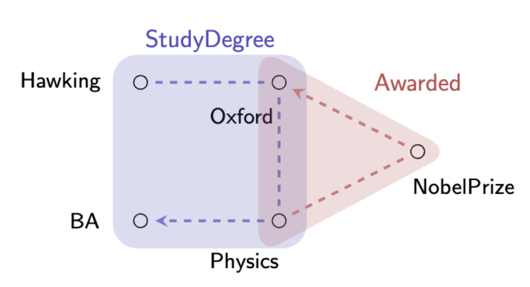
Figure 1: An example relational hypergraph. Each colored box represents a hyperedge connecting multiple entities, and the dashed arrow represents the specified order of entities in each relation.

Link prediction with relational hypergraphs, while valuable, poses significant challenges due to the varying numbers of nodes in each hyperedge. Most previous works focused on extending knowledge graph embedding methods to relational hypergraphs [8, 9], but they are all transductive, i.e., they cannot be directly applied to nodes unseen during training unlike inductive models. In a parallel, message-passing neural networks are extended to operate on relational hypergraphs [10, 11], but these architectures are only inductive if the node features are provided. In addition, our theoretical understanding of these message-passing architectures remains highly incomplete, leaving open questions about their expressiveness power.

To this end, we first define hypergraph relational message passing neural networks (HR-MPNNs) containing most of the message-passing neural networks proposed for relational hypergraphs [10, 11]. Following Barceló et al. [6], we quantify their expressive power through a relational Weisfeiler-Leman test. We also study the expressive power of HR-MPNNs in terms of logical formalisms, in the same spirit as Barceló et al. [12]. Inspired by the powerful conditional message passing paradigms studied in the context of knowledge graphs [5, 7], we introduce hypergraph conditional message passing neural networks (HC-MPNNs). HC-MPNNs are fully inductive even with the absence of input node features and can be seen as a strict generalization of the existing C-MPNN framework [7] on knowledge graphs. Through a careful comparison of the expressive power of HR-MPNNs and HC-MPNNs, we develop a systematic understanding of their capabilities and limitations.

We further propose a simple model instance of HC-MPNNs termed as hypergraph conditional networks (HCNets) and showcase its superior performances on both inductive and transductive link prediction tasks, followed by a detailed ablation study on its model components. Notably, HCNets are maximally expressive within HC-MPNNs and naturally subsume C-MPNNs, thus recovering models like NBFNets [5], when applied on knowledge graphs.

Our main contributions can be summarized as follows:

1. We investigate hypergraph relational message passing neural networks (HR-MPNNs) that encompass most of the existing architectures for link prediction with relational hypergraphs.

2. We build on the success of the conditional message passing paradigm in knowledge graphs and generalize this to relational hypergraphs leading to hypergraph conditional message passing neural networks (HC-MPNNs).

3. We study the expressive power in terms of distinguishing nodes of these architectures via corresponding WL algorithms. We also investigate their expressive power in terms of logics, namely, some hypergraph extensions of graded modal logic.

4. We conduct an empirical analysis for inductive link prediction with relational hypergraphs, surpassing existing baselines by a great margin. We further extend our analysis to transductive link prediction with relational hypergraphs and obtain state-of-the-art results.

5. We conduct a series of ablation studies on different model components justifying the importance of these components in the model predictions, and carry out additional experiments on knowledge graphs.

2 Related work

Knowledge graphs: Transductive setup. The task of link prediction on a knowledge graph has been studied extensively in the literature. The early knowledge graph embedding models such as TransE [13] and RotatE [14] are transductive. GNNs such as RGCN [4] and CompGCN [15] are prominent examples of utilizing powerful message-passing on knowledge graphs. However, none of these models apply in the fully inductive setup, where new nodes are introduced during the test time. This is because they inherently compute an embedding for each seen entity in the training graph.

Knowledge graphs: Inductive setup. GraIL [16] is the first model designed to be fully inductive by leveraging the idea of labeling trick [17]. GraIL labels each node with the shortest path distances to the source node and the target node in sampled subgraphs. However, such a method creates high computational complexity since in each forward pass, only one link score can be computed. Zhu et al. [5] proposed NBFNets, inspired by the Bellman-Ford algorithm, that allow the computation of $|V|$ links at the same time by only labeling the source node. NBFNets subsume many previous path-based models like NeuralLP [18] and DRUM [19]. These models fall under the framework of C-MPNNs [7] and are theoretically well-understood. Recently, A*Net [20] is designed to scale NBFNets with the usage of neural priority function, and Galkin et al. [21] proposed ULTRA, a foundation model that is inductive on both new nodes and new relation types, based on NBFNets. The success of conditional message passing on knowledge graphs has motivated us to extend its application to relational hypergraphs.

Relational hypergraphs: Transductive setup. There is a line of work focusing on adapting knowledge graph embedding methods for relational hypergraphs by extending the scoring function to consider multiple entities. For example, m-TransH [22], is an extension of TransH [23] designed to handle multiple entities simultaneously. Similarly, GETD [24] builds on the bilinear embedding method TuckER [25]. Fatemi et al. [9] proposed HSimplE and HypE that disentangle the position and relation embedding. BoxE [8] models each relation in terms of box embeddings, and naturally applies to $k$-ary relations while achieving strong results on transductive benchmarks. In addition, Fatemi et al. [26] drew a connection between relational algebra and relational hypergraph embedding and proposed ReAlE.

Relational hypergraphs: Inductive setup. As message-passing neural networks have shown great success in learning complex relational structures on graphs, Feng et al. [27] and Yadati et al. [28] leveraged message-passing methods on undirected hypergraphs. G-MPNN [10] is the first approach to specifically address multi-relational hypergraphs using message-passing. Building on this, RD-MPNNs [11] additionally incorporated the positional information of entities in their respective relations during message passing. They also explicitly keep track of the representations of the relation to better model the dynamics.

3 Link prediction with relational hypergraphs

Relational hypergraphs. A relational hypergraph $G=(V,E,R,c)$ consists of a set $E$ of hyperedges (or simply edges or facts) of the form $e=r(u_{1},\ldots,u_{k})\in E$ where $r\in R$ is a relation type, $u_{1},\ldots,u_{k}\in V$ are nodes, and $k=\mathtt{ar}(r)$ is the arity of the relation $r$. We consider labeled hypergraphs, where the labels are given by a coloring function on nodes $c:V\rightarrow D$. If the range of this coloring satisfies $D=\mathbb{R}^{d}$, we say $c$ is a $d$-dimensional feature map and use the notation ${\bm{x}}$ instead.

We write $\rho(e)$ to refer to the relation $r\in R$ of the hyperedge $e\in E$, and $e(i)$ to refer to the node in the $i$-th arity position of the hyperedge $e$. We define $E{(v)}$ as the set of edge-position pairs of a node $v$:

$$E{(v)}=\left\{(e,i)\mid e(i)=v,e\in E,1\leq i\leq\mathtt{ar}(\rho(e))\right\}.$$

Intuitively, this set captures all occurrences of node $v$ in different hyperedges and arity positions. We also define the positional neighborhood of an hyperedge $e$ with respect to a position $i$ as follows:

$${\mathcal{N}}_{i}(e)=\left\{(e(j),j)\mid j\neq i,1\leq j\leq\mathtt{ar}(\rho(e))\right\}.$$

This set represents all nodes that co-occur with the node at position $i$ in an hyperedge $e$, along with their positions. We refer to a knowledge graph as a special case of a relational hypergraph when all the edges have exactly arity $2$.

Link prediction on hyperedges. Given a relational hypergraph $G=(V,E,R,c)$, and a query $q(u_{1},...,u_{t-1},?,u_{t+1}...,u_{k})$, where $q\in R$ is the query relation and “$?$” is the querying position, link prediction is the problem of scoring all the hyperedges obtained by substituting nodes $v\in V$ in place of “$?$”. We denote a $k$-tuple $(u_{1},\ldots,u_{k})$ by ${\bm{u}}$ and the tuple $(u_{1},\ldots,u_{t-1},u_{t+1},\ldots,u_{k})$ by $\tilde{{\bm{u}}}$. For convenience, we commonly write a query as a tuple ${\bm{q}}=(q,\tilde{{\bm{u}}},t)$.

Isomorphisms. An isomorphism from a relational hypergraph ${G=(V,E,R,c)}$ to a relational hypergraph ${G^{\prime}=(V^{\prime},E^{\prime},R,c^{\prime})}$ is a bijection $f:V\to V^{\prime}$ such that $c(v)=c^{\prime}(f(v))$ for all $v\in V$, and $r(u_{1},\cdots,u_{k})\in E$ if and only if $r(f(u_{1}),\cdots,f(u_{k}))\in E^{\prime}$, for all $r\in R$ and $u_{1},\cdots,u_{k}\in V$.

Invariants. For $k\geq 1$, we define a k-ary relational hypergraph invariant as a function $\xi$ associating with each relational hypergraph $G=(V,E,R,c)$ a function $\xi(G)$ with domain $V^{k}$ such that for all relational hypergraphs $G,G^{\prime}$, all isomorphisms $f$ from $G$ to $G^{\prime}$, and for all $k$-tuples of nodes ${\bm{u}}\in V^{k}$, we have $\xi(G)({\bm{u}})=\xi(G^{\prime})(f({\bm{u}}))$.

Refinements. Given two relational hypergraph invariants $\xi$ and $\xi^{\prime}$, we say a function $\xi(G):V^{k}\to D$ refines a function $\xi^{\prime}(G):V^{k}\to D$, denoted as $\xi(G)\preceq\xi^{\prime}(G)$, if for all ${\bm{u}},{\bm{u}}^{\prime}\in V^{k}$, $\xi(G)({\bm{u}})=\xi(G)({\bm{u}}^{\prime})$ implies $\xi^{\prime}(G)({\bm{u}})=\xi^{\prime}(G)({\bm{u}}^{\prime})$. In addition, we call such functions equivalent, denoted as $\xi(G)\equiv\xi^{\prime}(G)$, if $\xi(G)\preceq\xi^{\prime}(G)$ and $\xi^{\prime}(G)\preceq\xi(G)$. A $k$-ary relational hypergraph invariant $\xi$ refines a $k$-ary relational hypergraph invariant $\xi^{\prime}$, if $\xi(G)$ refines $\xi^{\prime}(G)$ for all relational hypergraphs $G$. Similarly for equivalence.

4 Hypergraph relational MPNNs

We first introduce the framework of hypergraph relational message passing neural networks (HR-MPNNs), which capture existing message passing neural networks tailored for relational hypergraphs, such as G-MPNN [10] and RD-MPNN [11].

Let $G=(V,E,R,{\bm{x}})$ be a relational hypergraph, where ${\bm{x}}$ is a feature map that yields the initial node features ${\bm{x}}_{v}={\bm{x}}(v)$ for all nodes $v\in V$. For $\ell\geq 0$, an HR-MPNN iteratively computes a sequence of feature maps ${\bm{h}}^{(\ell)}:V\mapsto\mathbb{R}^{d(\ell)}$, where the representations ${\bm{h}}_{v}^{(\ell)}:={\bm{h}}^{(\ell)}(v)$ are given by:

$${\bm{h}}_{v}^{(0)} ={\bm{x}}_{v},$$

$${\bm{h}}_{v}^{(\ell+1)} =\textsc{up}\Big{(}{\bm{h}}_{v}^{(\ell)},\textsc{agg}\big{(}{\bm{h}}_{v}^{(\ell)},\{\!\!\{{\bm{m}}^{(\ell)}_{e,i}\mid(e,i)\in E(v)\}\!\!\}\big{)}\Big{)},$$

$${\bm{m}}^{(\ell)}_{e,i} =\textsc{msg}_{\rho(e)}\Big{(}\{({\bm{h}}_{w}^{(\ell)},j)\mid(w,j)\in{\mathcal{N}}_{i}(e)\}\Big{)},$$

where up, agg, and $\textsc{msg}_{\rho(e)}$ are differentiable, update, aggregation, and relation-specific message functions, respectively. These functions are layer-specific, but we omit the superscript $(\ell)$ for brevity. An HR-MPNN has a fixed number of layers $L\geq 0$ and the final representations of nodes are given by the function ${\bm{h}}^{(L)}:V\rightarrow\mathbb{R}^{d(L)}$. We can then use a $k$-ary decoder $\textsc{dec}_{q}:\mathbb{R}^{d(L)\times k}\rightarrow\mathbb{R}$, to produce a score for the likelihood of $q({\bm{u}})$ for $q\in R,{\bm{u}}\in V^{k}$.

HR-MPNNs contain MPNNs designed for single-relational, undirected hypergraphs, such as HGNN [27] and HyperGCN [28]. Furthermore, HR-MPNNs generalize R-MPNNs [7], defined in Appendix A, since a knowledge graph is a special case of a relational hypergraph.

4.1 HR-MPNNs and the Weisfeiler-Leman test

We formally characterize the expressive power of HR-MPNNs via a relational variant of the 1-dimensional Weisfeiler-Leman test on relational hypergraphs: the hypergraph relational 1-WL test, denoted by ${\sf hrwl}_{1}$. Note that ${\sf hrwl}_{1}$ serves as a natural generalization of ${\sf rwl}_{1}$ [6] on relational hypergraphs. Given a relational hypergraph $G=(V,E,R,c)$, for $\ell\geq 0$, ${\sf hrwl}_{1}$ updates the node colorings as follows:

$${\sf hrwl}_{1}^{(0)}(v) =c(v)$$

$${\sf hrwl}_{1}^{(\ell+1)}(v) =\tau\Big{(}{\sf hrwl}_{1}^{(\ell)}(v),\!\{\!\!\{\mathsf{col}^{(\ell)}(e,i)\!\mid\!(e,i)\!\in\!E(v)\}\!\!\}\Big{)}$$

$$\mathsf{col}^{(\ell)}(e,i) =\big{(}\{({\sf hrwl}_{1}^{(\ell)}(w),j)\!\mid(w,j)\in{\mathcal{N}}_{i}(e)\},\rho(e)\big{)}.$$

The function $\tau$ is an injective mapping that maps the above pair to a unique color that has not been used in previous iterations. Note that ${\sf hrwl}_{1}^{(\ell)}$ defines a valid node invariant on relational hypergraphs for all $\ell\geq 0$. As it turns out, ${\sf hrwl}_{1}$ has the same expressive power as HR-MPNNs in terms of distinguishing nodes:

Theorem 4.1.

Let $G=(V,E,R,c)$ be a relational hypergraph, then the following statements hold:

1. For all initial feature maps ${\bm{x}}$ with $c\equiv{\bm{x}}$, all HR-MPNNs with $L$ layers, and for all $0\leq\ell\leq L$, it holds that ${\sf hrwl}_{1}^{(\ell)}\preceq{\bm{h}}^{(\ell)}$.

2. For all $L\geq 0$, there is an initial feature map ${\bm{x}}$ with $c\equiv{\bm{x}}$ and an HR-MPNN with $L$ layers, such that for all $0\leq\ell\leq L$, we have ${\sf hrwl}_{1}^{(\ell)}\equiv{\bm{h}}^{(\ell)}$.

Intuitively, item (1) states that ${\sf hrwl}_{1}$ upper bounds the power of any HR-MPNN: if the test cannot distinguish two nodes, then the HR-MPNN cannot either. On the other hand, item (2) states that HR-MPNNs can be as expressive as ${\sf hrwl}_{1}$: for any $L$, there is an HR-MPNN that simulates $L$ iterations of the test. In our proof, we explicitly construct this HR-MPNN using a simple architecture (see Appendix B).

4.2 HR-MPNNs and logics

The previous WL characterization of HR-MPNNs is non-uniform in the sense that it holds for a given fixed relational hypergraph $G$. We now turn our attention to a uniform analysis of the power of HR-MPNNs and study the problem of which (node) classifiers can be expressed as HR-MPNNs. Following Barceló et al. [12], we investigate logical classifiers, i.e., those that can be defined in the formalism of first-order logic (FO). Briefly, a first-order formula $\phi(x)$ with one free variable $x$ defines a logical classifier that assigns value ${\sf true}$ to node $u$ in relational hypergraph $G$ whenever $G\models\phi(u)$. A logical classifier $\phi(x)$ is captured by a HR-MPNN $\cal A$ if for every relational hypergraph $G$ the nodes $u$ that are classified as ${\sf true}$ by $\phi$ and $\cal A$ are the same.

It was shown in Barceló et al. [12] that a logical classifier is captured by a GNN over single-relational graphs if and only if it can be expressed in graded modal logic [29, 30]. This result was later extended to multi-relational graphs in Huang et al. [7]. Here we consider a variant of graded modal logic for hypergraphs. Fix a set of relation types $R$ and a set of node colors $\mathcal{C}$. The hypergraph graded modal logic (HGML) is the fragment of FO containing the following unary formulas. Firstly, $a(x)$ for $a\in\mathcal{C}$ is a formula. Secondly, if $\varphi(x)$ and $\varphi^{\prime}(x)$ are HGML formulas, then $\neg\varphi(x)$ and $\varphi(x)\land\varphi^{\prime}(x)$ also are. Thirdly, for $r\in R$, $1\leq i\leq{\textsf{ar}}(r)$ and $N\geq 1$:

$$\exists^{\geq N}\tilde{{\bm{y}}}\,\Big{(}r(y_{1},\dots,y_{i-1},x,y_{i+1},\dots,y_{{\textsf{ar}}(r)})\land\Psi(\tilde{{\bm{y}}})\Big{)}$$

is a HGML formula, where $\tilde{{\bm{y}}}=(y_{1},\dots,y_{i-1},y_{i+1},\dots,y_{{\textsf{ar}}(r)})$ and $\Psi(\tilde{{\bm{y}}})$ is a boolean combination of HGML formulas having free variables from $\tilde{{\bm{y}}}$. Intuitively, the formula expresses that $x$ participates in at least $N$ edges $e$ at position $i$, such that the remaining nodes in $e$ satisfy $\Psi$. Interestingly, we can show that HR-MPNNs are as powerful as HGML (see Appendix C for details):

Theorem 4.2.

Each hypergraph graded modal logic classifier is captured by a HR-MPNN.

We leave the converse as an open problem, i.e., whether HR-MPNNs only capture HGML classifiers. Following Barceló et al. [12], this may require extending bisimulation results from Otto [31] to hypergraphs.

5 Hypergraph conditional MPNNs

In this section, we propose hypergraph conditional message passing networks (HC-MPNNs), a generalization of C-MPNNs [7] to relational hypergraphs.

Let $G=(V,E,R,{\bm{x}})$ be a relational hypergraph, where ${\bm{x}}$ is a feature map. Given a query ${\bm{q}}=(q,\tilde{{\bm{u}}},t)$, for $\ell\geq 0$, an HC-MPNN computes a sequence of feature maps ${\bm{h}}_{v|{\bm{q}}}^{(\ell)}$ as follows:

$${\bm{h}}_{v|{\bm{q}}}^{(0)} =\textsc{init}(v,{\bm{q}}),$$

$${\bm{h}}_{v|{\bm{q}}}^{(\ell+1)} =\textsc{up}\Big{(}{\bm{h}}_{v|{\bm{q}}}^{(\ell)},\textsc{agg}\big{(}{\bm{h}}_{v|{\bm{q}}}^{(\ell)},\{\!\!\{{\bm{m}}_{e,i|{\bm{q}}}^{(\ell)}\mid(e,i)\in E(v)\}\!\!\}\big{)}\Big{)},$$

$${\bm{m}}_{e,i|{\bm{q}}}^{(\ell)} =\textsc{msg}_{\rho(e)}\left(\{({\bm{h}}_{w|{\bm{q}}}^{(\ell)},j)\mid(w,j)\in{\mathcal{N}}_{i}(e)\},{\bm{q}}\right),$$

where init, up, agg, and $\textsc{msg}_{\rho(e)}$ are differentiable initialization, update, aggregation, and relation-specific message functions, respectively. An HC-MPNN has a fixed number of layers $L\geq 0$, and the final conditional node representation are given by ${\bm{h}}_{v|{\bm{q}}}^{(L)}$. We denote by ${\bm{h}}^{(\ell)}_{\bm{q}}:V\rightarrow\mathbb{R}^{d(\ell)}$ the function ${\bm{h}}^{(\ell)}_{\bm{q}}(v):={\bm{h}}_{v|{\bm{q}}}^{(\ell)}$.

To ensure that HC-MPNNs compute $k$-ary representations, we impose a generalized version of target node distinguishability proposed by Huang et al. [7]. We say an initialization function init satisfies generalized target node distinguishability if for all ${\bm{q}}=(q,\tilde{{\bm{u}}},t)$, the following conditions hold:

$$\textsc{init}(u,{\bm{q}}) \neq\textsc{init}(v,{\bm{q}})\quad\forall u\in\tilde{{\bm{u}}},v\notin\tilde{{\bm{u}}}$$

$$\textsc{init}(u_{i},{\bm{q}}) \neq\textsc{init}(u_{j},{\bm{q}})\quad\forall u_{i},u_{j}\in\tilde{{\bm{u}}},u_{i}\neq u_{j}.$$

Different from message passing on simple hypergraphs, we need to consider the relation type of each edge (multi-relational) and the relative position of each node (directed) in the edges on relational hypergraphs. Therefore, the message function $\textsc{msg}_{\rho(e)}$ needs to be relation-specific while also keeping track of the positions $j$ of nodes $w$ in their respective neighborhoods ${\mathcal{N}}_{i}(e)$. We can then obtain the scores of query ${\bm{q}}$ applying a unary decoder dec on ${\bm{h}}_{v|{\bm{q}}}^{(L)}$.

5.1 Hypergraph conditional networks

In this section, we define concrete model architecture, but let us first introduce some notation.

Notation. Let us denote by ${\bm{z}}_{q}$ a learnable query-specific vector for $q\in R$, and by $\|$ row concatenation. Let $\mathbbm{1}_{C}$ be the indicator function that returns $1$ if condition $C$ is true, and $0$ otherwise. As usual, $*$ is scalar multiplication, and $\odot$ is element-wise multiplication of vectors. We write $\alpha$ to refer to a learnable scalar. Finally, we follow the usual convention and write ${\bm{p}}_{i}$ to represent the positional encoding at position $i$.

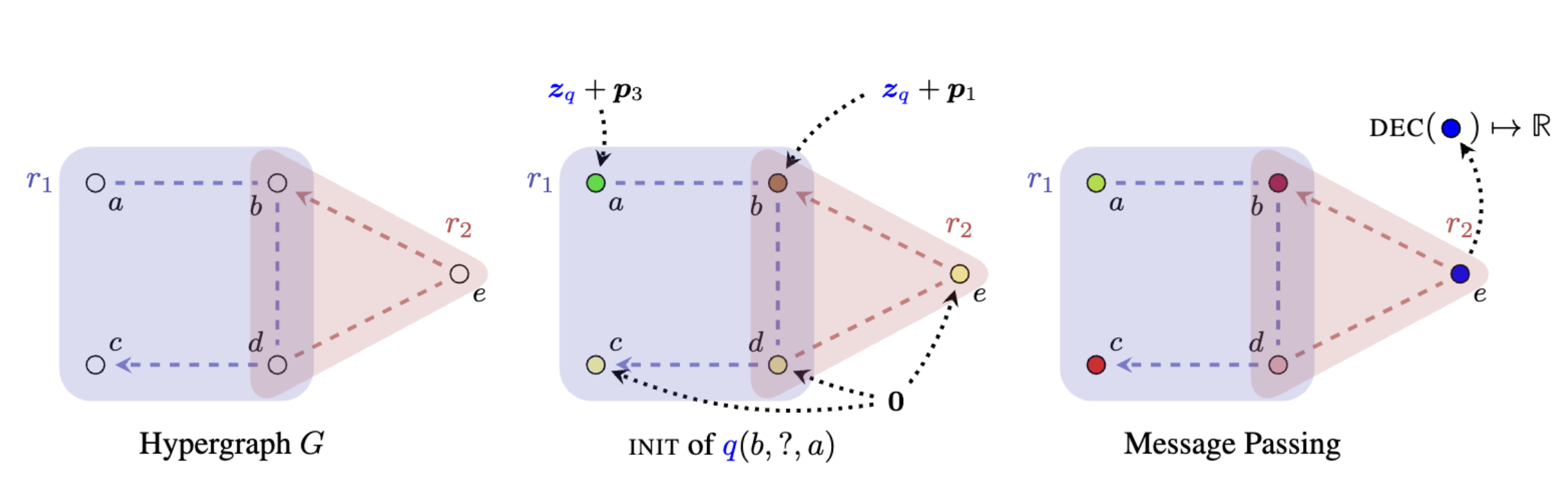
Figure 2: Visualization of HCNet on relational hypergraph $G$ with $V=\{a,b,c,d,e\}$, $E=\{r_{1}(a,b,d,c),r_{2}(d,e,b)\}$, $R=\{r_{1},r_{2}\}$. We ask the query $q(b,?,a)$, and show the computation of the score for $q(b,e,a)$. Here, ${\bm{z}}_{q}$ is the learnable relation vector for query relation $q\in R$, and ${\bm{p}}_{i}$ is the positional encoding of the $i$-th arity position.

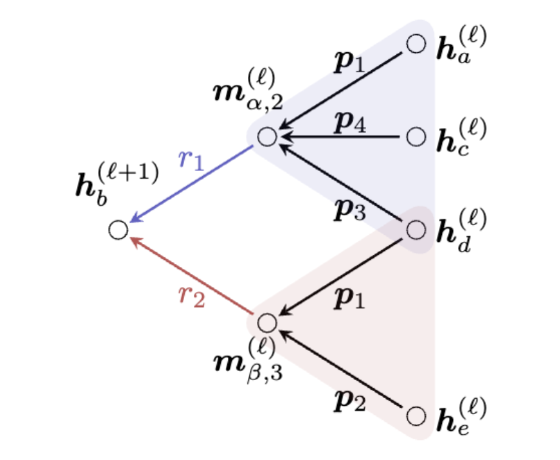
Figure 3: Computational graph of HCNet on node $b$ in relational hypergraph $G$ at layer $\ell$, where ${\alpha=r_{1}(a,b,d,c)}$ and ${\beta=r_{2}(d,e,b)}$. Here, we omit self-transformation on ${\bm{h}}_{b}^{(\ell)}$ here for ease of presentation.

HCNets. We define a basic instance of HC-MPNNs, which we call hypergraph conditional networks (HCNets). For a query ${\bm{q}}=(q,\tilde{{\bm{u}}},t)$, an HCNet computes the following representations for all $\ell\geq 0$:

$${\bm{h}}_{v|{\bm{q}}}^{(0)} =\sum_{i\neq t}\mathbbm{1}_{v=u_{i}}*({\bm{p}}_{i}+{\bm{z}}_{q})$$

$${\bm{h}}_{v|{\bm{q}}}^{(\ell+1)} =f^{(\ell)}\Big{(}\Big{[}{\bm{h}}_{v|{\bm{q}}}^{(\ell)}\Big{\|}\sum_{(e,i)\in E(v)}{\bm{m}}^{(\ell)}_{e,i|{\bm{q}}}\Big{]}\Big{)}$$

$${\bm{m}}^{(\ell)}_{e,i|{\bm{q}}} =g_{\rho(e),q}^{(\ell)}\Big{(}\odot_{j\neq i}(\alpha^{(\ell)}{\bm{h}}_{e(j)|{\bm{q}}}^{(\ell)}\!\!+(1-\alpha^{(\ell)}){\bm{p}}_{j})\Big{)}.$$

In our experiments, we fix $f^{(\ell)}$ to be a linear map (with bias) followed by a nonlinearity. Moreover, we set $g_{\rho(e),q}^{(\ell)}$ to be a diagonal linear map $\operatorname{Diag}({\bm{b}}_{r,q})$ where ${\bm{b}}_{r,q}$ can be (1) query-dependent, i.e., ${\bm{b}}_{r,q}={\bm{W}}_{r}{\bm{z}}_{q}$ where ${\bm{W}}_{r}$ is a learnable matrix for each relation $r$, or (2) query-independent, i.e., ${\bm{b}}_{r,q}={\bm{b}}_{r}$ where ${\bm{b}}_{r}$ is a learnable vector for each relation $r$. Note that these functions can be $2$-layer MLPs in their full generality. As for our experiments, we consider sinusoidal positional encoding defined by Vaswani et al. [32].

Intuitively, the model initialization ensures that all source nodes (i.e., nodes that appear in $\tilde{{\bm{u}}}$) are initialized to their respective positions in the query edge, and all other nodes are initialized as the zero vector $\mathbf{0}$. The visualization of HCNet is shown in Figure 2, and the corresponding computational graph of HCNet at each updating step $\ell$ is shown in Figure 3. Furthermore, we provide a detailed discussion of computational complexity between HR-MPNNs and HC-MPNNs in Table 5.

5.2 Expressive power of HC-MPNNs

5.2.1 A Weisfeiler-Leman characterization

To analyze the expressive power of HC-MPNNs for distinguishing nodes, we can still use the ${\sf hrwl}_{1}$ test provided we restrict ourselves to initial colorings $c$ that respect the given query ${\bm{q}}$. Formally, given a query ${\bm{q}}=(q,\tilde{{\bm{u}}},t)$ on a relational hypergraph $G=(V,E,R,c)$, we say that the coloring $c$ satisfies generalized target node distinguishability with respect to ${\bm{q}}$ if:

$$c(u) \neq c(v)\quad\forall u\in\tilde{{\bm{u}}},v\notin\tilde{{\bm{u}}}$$

$$c(u_{i}) \neq c(u_{j})\quad\forall u_{i},u_{j}\in\tilde{{\bm{u}}},u_{i}\neq u_{j}.$$

Note that initial colorings satisfying this property are equivalent to the initializations of HC-MPNNs. As a direct consequence of Theorem 4.1 we obtain (see Appendix D):

Theorem 5.1.

Let $G=(V,E,R,c)$ be a relational hypergraph and ${\bm{q}}=(q,\tilde{{\bm{u}}},t)$ be a query such that $c$ satisfies generalized target node distinguishability with respect to ${\bm{q}}$. Then the following statements hold:

1. For all HC-MPNNs with $L$ layers and initializations init with $\textsc{init}\equiv c$, $0\leq\ell\leq L$ , ${\sf hrwl}_{1}^{(\ell)}\preceq{\bm{h}}_{\bm{q}}^{(\ell)}$ holds.

2. For all $L\geq 0$ , there is an HC-MPNN with $L$ layers such that for all $0\leq\ell\leq L$ , we have ${\sf hrwl}_{1}^{(\ell)}\equiv{\bm{h}}_{\bm{q}}^{(\ell)}$.

Theorem 5.1 tells us that HC-MPNNs are stronger than HR-MPNNs due to its initialization: HC-MPNNs can initialize nodes differently based on the query ${\bm{q}}$, whereas HR-MPNNs always assign the same initialization for all queries.

5.2.2 HC-MPNNs and logics

We remark that Theorem 4.2 can be translated to HC-MPNNs by slightly modifying the logic. We consider symbolic queries ${\bm{q}}=(q,\tilde{{\bm{b}}},t)$, where now each $b\in\tilde{{\bm{b}}}$ is a constant symbol. Our vocabulary contains relation types $r\in R$ and node colors ${\cal C}$, as before, and additionally the constants $b\in\tilde{{\bm{b}}}$. We define hypergraph graded modal logic with constants (HGML_c) as HGML but, as atomic cases, we additionally have formulas of the form $\varphi(x)=(x=b)$ for some constant $b$. In Appendix E we show that each HGML_c classifier can be captured by an HC-MPNN.

5.2.3 Link prediction with knowledge graphs

An interesting observation is that when we restrict relational hypergraphs to have hyperedges of arity exactly $2$, we recover the class of knowledge graphs. C-MPNNs [7] are tailored for knowledge graphs and their expressive power has been recently studied extensively, with a focus on their capability for distinguishing pairs of nodes (for a formal definition see Appendix A). In this section, we compare HC-MPNNs and C-MPNNs, and hence we are interested in the expressive power of HC-MPNNs in terms of distinguishing pairs of nodes. Note however that, in principle, HC-MPNNs do not compute binary invariants. Indeed, for $q\in R$ and a pair of nodes $u,v$ we can obtain two final features depending on whether we pose the query $q(u,?)$ or $q(?,v)$. As a convention, we shall define the final feature of the pair $u,v$ as the result of the query $q(u,?)$. When a HC-MPNN computes binary invariants under this convention, we say the HC-MPNN is restricted to tail predictions.

In Appendix F we show that HC-MPNNs restricted to tail predictions has the same expressive power in terms of distinguishing pairs of nodes as the ${\sf rawl}_{2}^{+}$ test proposed in Huang et al. [7]. This test is an extension of ${\sf rawl}_{2}$, which in turn, matches the expressive power of C-MPNNs. It follows then that HC-MPNNs are strictly more powerful than C-MPNNs over knowledge graphs.

We remark that the idea of HC-MPNNs restricted to tail predictions can be extended to arbitrary relational hypergraphs in order to compute $k$-ary invariants for any $k$. See Appendix H for a discussion.

6 Experimental evaluation

We evaluate HCNet in two settings, namely inductive link prediction and transductive link prediction with relational hypergraphs. We further carry out analysis on different arities to emphasize the effectiveness of higher-arity relation, and ablation study on initialization and positional encoding of HCNets. In addition, we show empirical results that when restricted to knowledge graphs, HCNets still produce competitive results compared to state-of-the-art models in Appendix I.

Empirical setups. In all experiments, we consider a 2-layer MLP as the decoder and adopt layer normalization and dropout in all layers before applying ReLU activation and skip-connection. During the training, we remove edges that are currently being treated as positive tuples to prevent overfitting for each batch. We choose the best checkpoint based on its evaluation of the validation set. In terms of evaluation, we adopt filtered ranking protocol. For each test edge $q(u_{1},\ldots,u_{k})$ where $k={\textsf{ar}}(q)$, and for each arity $t\in\{1,...,k\}$, we replace the $t$-th entities by all other possible entities such that the query after replacement is not in the graph. We report Mean Reciprocal Rank(MRR) and Hits@$k$ where $k=1,3$ in inductive experiments and additionally $k=10$ in transductive experiments as evaluation metrics and provide averaged results of five runs on different seeds. We ran all the experiments on a single NVIDIA V100 GPU, and reported experiment details in Appendix K. The code for experiments is provided in https://anonymous.4open.science/r/HC-MPNN.

Table 1: Results of inductive link prediction experiments. We report MRR, Hits@$1$, and Hits@$3$ (higher is better) on test sets.

	WP-IND			JF-IND			MFB-IND
	MRR	Hits@1	Hits@3	MRR	Hits@1	Hits@3	MRR	Hits@1	Hits@3
HGNN	0.072	0.045	0.112	0.102	0.086	0.128	0.121	0.076	0.114
HyperGCN	0.075	0.049	0.111	0.099	0.088	0.133	0.118	0.074	0.117
G-MPNN-sum	0.177	0.108	0.191	0.219	0.155	0.236	0.124	0.071	0.123
G-MPNN-mean	0.153	0.096	0.145	0.112	0.039	0.116	0.241	0.162	0.257
G-MPNN-max	0.200	0.125	0.214	0.216	0.147	0.240	0.268	0.191	0.283
HCNet	0.414	0.352	0.451	0.435	0.357	0.495	0.368	0.223	0.417

Table 2: Results of transductive link prediction experiments. We report MRR, Hits@1, Hits@3, and Hits@10 (higher is better) on test sets.

	JF17K				FB-AUTO
	MRR	Hits@1	Hits@3	Hits@10	MRR	Hits@1	Hits@3	Hits@10
r-SimplE	0.102	0.069	0.112	0.168	0.106	0.082	0.115	0.147
m-DistMult	0.463	0.372	0.510	0.634	0.784	0.745	0.815	0.845
m-CP	0.391	0.298	0.443	0.563	0.752	0.704	0.785	0.837
m-TransH	0.444	0.370	0.475	0.581	0.728	0.727	0.728	0.728
HSimplE	0.472	0.378	0.520	0.645	0.798	0.766	0.821	0.855
HypE	0.494	0.408	0.538	0.656	0.804	0.774	0.823	0.856
GETD	0.151	0.104	0.151	0.258	0.367	0.254	0.422	0.601
BoxE	0.560	0.472	0.604	0.722	0.844	0.814	0.863	0.898
ReAIE	0.530	0.454	0.563	0.677	0.861	0.836	0.877	0.908
RD-MPNN	0.512	0.445	0.573	0.685	0.810	0.714	0.880	0.888
HCNet	0.525	0.427	0.574	0.718	0.871	0.842	0.892	0.922

6.1 Inductive experiments

Datasets. Yadati [10] constructed three inductive datasets, WP-IND, JF-IND, and MFB-IND from existing transductive datasets: Wikipeople [33], JF17K [22], and M-FB15K [9], respectively, where the test sets contain unseen entities during training. We report their statistics in Table 10, Appendix K.

Baselines. We compare with the baseline models HGNN [27], HyperGCN [28], and three variants of G-MPNN [10] with different aggregation functions, provided in Table 1. Note that since HGNN and HyperGCN are designed for simple hypergraphs with no relations, Yadati [10] tested them on transformed relational hypergraphs where the relation information is ignored. In addition, Yadati [10] initialized nodes with given node features, whereas we ignore the node feature and initialize each node with the respective initialization defined in HCNets. We adopt the query-independent message function in all inductive experiments, and the batching trick on MFB-IND following Zhu et al. [5]. All the hyper-parameter considered is reported in Table 12, Appendix K.

Results. We report the inductive experiments results in Table 1, and observe that HCNet outperforms all the existing baseline methods by a large margin, doubling the metric on WP-IND and JF-IND and substantially increasing on MFB-IND. Notably, we emphasize that HCNet does not utilize the provided node features whereas other baseline models do, further highlighting the effectiveness of HCNet in generalizing to entirely new graphs in the absence of node features. This is because HCNet is more expressive by computing query-dependent unary invariants instead of query-agnostic unary invariants as G-MPNNs (with different aggregation functions), which are all instances of HR-MPNNs. Overall these results perfectly align with the main theoretical findings presented in this paper.

Table 3: Results of ablation study experiments on initialization. We report MRR and Hits@$3$ (higher is better) on test sets.

init		WP-IND		JF-IND
${\bm{z}}_{q}$	${\bm{p}}_{i}$	MRR	Hits@3	MRR	Hits@3
-	-	0.388	0.421	0.390	0.451
✓	-	0.387	0.421	0.392	0.447
-	✓	0.394	0.430	0.393	0.456
✓	✓	0.414	0.451	0.435	0.495

Table 4: Results of ablation study experiments on positional encoding. We report MRR and Hits@$3$ (higher is better) on test sets.

PE	WP-IND		JF-IND
	MRR	Hits@3	MRR	Hits@3
Constant	0.393	0.426	0.356	0.428
One-hot	0.395	0.428	0.368	0.432
Learnable	0.396	0.425	0.416	0.480
Sinusoidal	0.414	0.451	0.435	0.495

6.2 Transductive experiments

Datasets & Baselines. We evaluate HCNets on the link prediction task with relational hypergraphs, namely the publicly available JF17K [22] and FB-AUTO [9]. These datasets include facts of different arities up to $6$. We have taken the results of r-SimplE, m-DistMult, m-CP, HSimplE, HypE, and m-TransH [22] from Fatemi et al. [9], BoxE from Abboud et al. [8], and GETD [24], ReAIE [26], RD-MPNN from Zhou et al. [11]. We consider the query-dependent message function in all experiments with JF17K, and the query-independent message function on FB-AUTO. The statistics of the datasets are reported in Table 11, and the hyper-parameter choices in Table 13. We also analyze the performance when testing with different arities on JF17K, reported in Table 9, Appendix J.

Results. We summarize the results for the transductive link prediction tasks and report them in Table 2. HCNet is placed top in FB-AUTO on all metrics and is very competitive in JF17K, where it is top 2 in Hits@$3$ and Hits@$10$, outperforming most of the existing methods except BoxE, which is designed specifically for transductive setting. In particular, we observe that on almost all metrics in both datasets, HCNet outperforms RD-MPNN, an HR-MPNN instance, empirically validating our theory and proving that HCNet is effective in transductive setting.

6.3 Ablation study

To further assess the contribution of each model component, we carry out an ablation study, mainly on different choices of positional encoding and initialization functions. The ablation study is carried out on WP-IND and JF-IND datasets with the same empirical setup described in Section 6.1 and with the same hyperparameters shown in Table 12. The detailed definitions of model variants considered in the ablation study are reported in Appendix K.

Initialization. To validate the impact of different initialization schemes, we conduct experiments, which are reported in Table 3. We evaluate all combinations including positional encoding and learnable query vectors.

We observe that both positional encoding ${\bm{p}}_{i}$ and the relation ${\bm{z}}_{q}$ are essential in the initialization as removing either of them worsens the overall performance of HCNet. A closer look reveals that the removal of the positional information is more detrimental compared to relational information since the model could deduce the relation types based on implicit information such as the arity of the query relation.

Positional encoding. We examine the importance of the choice of positional encoding, which serves as an indicator of which position the given entities lie in an hyperedge. We provide experiments on multiple choices of positional encodings, and report the results in Table 4.

We show that the sinusoidal positional encoding produces the best results, possibly due to its ability to measure sequential dependency between neighboring entities, compared with one-hot positional encoding which assumes orthogonality among each position. We also notice that learnable embeddings do not produce better results since it is generally hard to learn a suitable embedding that respects the order of the nodes in a relation as they are initialized randomly. Finally, constant embedding evidently performs the worst as it pays no respect to position information and treats all hyperedges with the same set of nodes in the same way regardless of the order of the nodes in these edges.

7 Conclusion

We investigated two frameworks of relational message-passing neural networks on the task of link prediction with relational hypergraphs, namely HR-MPNNs and HC-MPNNs. Furthermore, we studied the expressive power of these two frameworks in terms of relational WL and logical formalism. We then proposed a simple yet powerful model instance of HC-MPNNs called HCNet and presented its superior performance on both inductive and transductive link prediction tasks. One limitation lies in the potentially high computational complexity when applying to large complex relational hypergraphs. Further research is needed to optimize these models for scalability. Our study extends the success of link prediction with knowledge graphs to relational hypergraphs where higher arity relations can be effectively modeled with GNNs, unlocking applications in fully relational structures.

Appendix A R-MPNNs and C-MPNNs

In this section, we define relational message passing neural networks (R-MPNNs) and conditional message passing neural networks (C-MPNNs) following Huang et al. [7]. For ease of presentation, we omit the discussion regarding history functions and readout functions from Huang et al. [7].

R-MPNNs. Let $G=(V,E,R,{\bm{x}})$ be a knowledge graph, where ${\bm{x}}$ is a feature map. A relational message passing neural network (R-MPNN) computes a sequence of feature maps ${\bm{h}}^{(\ell)}:V\to\mathbb{R}^{d(\ell)}$, for $\ell\geq 0$. For simplicity, we write ${\bm{h}}^{(\ell)}_{v}$ instead of ${\bm{h}}^{(\ell)}(v)$. For each node $v\in V$, the representations ${\bm{h}}^{(\ell)}_{v}$ are iteratively computed as:

$${\bm{h}}_{v}^{(0)} ={\bm{x}}_{v}$$

$${\bm{h}}_{v}^{(\ell+1)} =\ \textsc{up}\left({\bm{h}}_{v}^{(\ell)},\textsc{agg}(\{\!\!\{\textsc{msg}_{r}({\bm{h}}_{w}^{(\ell)})|~{}w\in\mathcal{N}_{r}(v),r\in R\}\!\!\})\right),$$

where up, agg, and $\textsc{msg}_{r}$ are differentiable update, aggregation, and relation-specific message functions, respectively, $\mathcal{N}_{r}(v):=\{u\mid r(u,v)\in E\}$ is the neighborhood of a node $v\in V$ relative to a relation $r\in R$. An R-MPNN has a fixed number of layers $L\geq 0$, and then, the final node representations are given by the map ${\bm{h}}^{(L)}:V\to\mathbb{R}^{d(L)}$. The final representations can be used for node-level predictions. For link-level tasks, we use a binary decoder ${\textsc{dec}_{q}:\mathbb{R}^{d(L)}\times\mathbb{R}^{d(L)}\to{\mathbb{R}}}$, which produces a score for the likelihood of the fact $q(u,v)$, for $q\in R$.

C-MPNNs. Let $G=(V,E,R,{\bm{x}})$ be a knowledge graph, where ${\bm{x}}$ is a feature map. A conditional message passing neural network (C-MPNN) iteratively computes pairwise representations, relative to a fixed query $q\in R$ and a fixed node $u\in V$, as follows:

$${\bm{h}}_{v|u,q}^{(0)} =\textsc{init}(u,v,q)$$

$${\bm{h}}_{v|u,q}^{(\ell+1)} =\textsc{up}\Big{(}{\bm{h}}_{v|u,q}^{(\ell)},\textsc{agg}(\{\!\!\{\textsc{msg}_{r}({\bm{h}}_{w|u,q}^{(\ell)},{\bm{z}}_{q})|~{}w\in\mathcal{N}_{r}(v),r\in R\}\!\!\})\Big{)},$$

where init, up, agg, and $\textsc{msg}_{r}$ are differentiable initialization, update, aggregation, and relation-specific message functions, respectively.

We denote by ${\bm{h}}_{q}^{(\ell)}:V\times V\to\mathbb{R}^{d(\ell)}$ the function ${\bm{h}}_{q}^{(\ell)}(u,v):={\bm{h}}_{v|u,q}^{(\ell)}$, and denote ${\bm{z}}_{q}$ to be a learnable vector representing the query $q\in R$. A C-MPNN has a fixed number of layers $L\geq 0$, and the final pair representations are given by ${\bm{h}}_{q}^{(L)}$. To decode the likelihood of the fact $q(u,v)$ for some $q\in R$, we simply use a unary decoder $\textsc{dec}:\mathbb{R}^{d(L)}\to{\mathbb{R}}$, parameterized by a 2-layer MLP. In addition, we require $\textsc{init}(u,v,q)$ to satisfy target node distinguishability: for all $q\in R$ and $v\neq u\in V$, it holds that $\textsc{init}(u,u,q)\neq\textsc{init}(u,v,q)$.

Appendix B Missing details from Section 4.1

Theorem 4.1.

Let $G=(V,E,R,c)$ be a relational hypergraph, then the following statements hold:

1. For all initial feature maps ${\bm{x}}$ with $c\equiv{\bm{x}}$, all HR-MPNNs with $L$ layers, and for all $0\leq\ell\leq L$, it holds that ${\sf hrwl}_{1}^{(\ell)}\preceq{\bm{h}}^{(\ell)}$.

2. For all $L\geq 0$, there is an initial feature map ${\bm{x}}$ with $c\equiv{\bm{x}}$ and an HR-MPNN with $L$ layers, such that for all $0\leq\ell\leq L$, we have ${\sf hrwl}_{1}^{(\ell)}\equiv{\bm{h}}^{(\ell)}$.

Proof.

To prove item (1), we first take an initial feature map ${\bm{x}}$ with $c\equiv{\bm{x}}$ and a HR-MPNN with $L$ layers. We apply induction on $\ell$. The base case where $\ell=0$ follows directly as ${\sf hrwl}_{1}^{(0)}\equiv c\equiv{\bm{x}}\equiv{\bm{h}}^{(0)}$. For the inductive case, assume ${\sf hrwl}_{1}^{(\ell+1)}(u)={\sf hrwl}_{1}^{(\ell+1)}(v)$ for some node pair $u,v\in V$ and for some $\ell\geq 1$. By injectivity of $\tau$, it follows that ${\sf hrwl}_{1}^{(\ell)}(u)={\sf hrwl}_{1}^{(\ell)}(v)$ and

$$\{\!\!\{(\{({\sf hrwl}_{1}^{(\ell)}(w),j)\mid(w,j)\in{\mathcal{N}}_{i}(e)\},\rho(e))\mid(e,i)\in E(u)\}\!\!\}=$$

$$\{\!\!\{(\{({\sf hrwl}_{1}^{(\ell)}(w),j)\mid(w,j)\in{\mathcal{N}}_{i^{\prime}}(e^{\prime})\},\rho(e^{\prime}))\mid(e^{\prime},i^{\prime})\in E(v)\}\!\!\}$$

By inductive hypothesis, we have:

$${\bm{h}}_{u}^{(\ell)} ={\bm{h}}_{v}^{(\ell)}$$

$$\{\!\!\{(\{({\bm{h}}_{w}^{(\ell)},j)\mid(w,j)\in{\mathcal{N}}_{i}(e)\},\rho(e))\mid(e,i)\in E(u)\}\!\!\} =\{\!\!\{(\{({\bm{h}}_{w}^{(\ell)},j)\mid(w,j)\in{\mathcal{N}}_{i^{\prime}}(e^{\prime})\},\rho(e^{\prime}))\mid(e^{\prime},i^{\prime})\in E(v)\}\!\!\}.$$

Thus we have

$$\{\!\!\{\textsc{msg}_{\rho(e)}^{(\ell)}\Big{(}\{({\bm{h}}_{w}^{(\ell)},j)\mid(w,j)\in{\mathcal{N}}_{i}(e)\}\Big{)}\mid(e,i)\in E(u)\}\!\!\} =\{\!\!\{\textsc{msg}_{\rho(e^{\prime})}^{(\ell)}\Big{(}\{({\bm{h}}_{w}^{(\ell)},j)\mid(w,j)\in{\mathcal{N}}_{i^{\prime}}(e^{\prime})\}\Big{)}\mid(e^{\prime},i^{\prime})\in E(v)\}\!\!\}$$

and then:

$$\{\!\!\{{\bm{m}}_{e,i}^{(\ell)}\mid(e,i)\in E(u)\}\!\!\} =\{\!\!\{{\bm{m}}_{e^{\prime},i^{\prime}}^{(\ell)}\mid(e^{\prime},i^{\prime})\in E(v)\}\!\!\}.$$

We thus conclude that

$${\bm{h}}_{u}^{(\ell+1)} =\textsc{up}^{(\ell)}\Big{(}{\bm{h}}_{u}^{(\ell)},\textsc{agg}\Big{(}{\bm{h}}_{u}^{(\ell)},\{\!\!\{{\bm{m}}^{(\ell)}_{e,i}\mid(e,i)\in E(u)\}\!\!\}\Big{)}\Big{)}$$

$$=\textsc{up}^{(\ell)}\Big{(}{\bm{h}}_{v}^{(\ell)},\textsc{agg}\Big{(}{\bm{h}}_{v}^{(\ell)},\{\!\!\{{\bm{m}}^{(\ell)}_{e^{\prime},i^{\prime}}\mid(e^{\prime},i^{\prime})\in E(v)\}\!\!\}\Big{)}\Big{)}$$

$$={\bm{h}}_{v}^{(\ell+1)}.$$

Now we proceed to show item (2). We use a model of HR-MPNN in the following form and show that any iteration of ${\sf hrwl}_{1}$ can be simulated by a specific layer of such instance of HR-MPNN:

$${\bm{h}}_{v}^{(0)} ={\bm{x}}_{v}$$

$${\bm{h}}_{v}^{(\ell+1)} =f^{(\ell)}\Big{(}\Big{[}{\bm{h}}_{v}^{(\ell)}\Big{\|}\sum_{(e,i)\in E(v)}g_{\rho(e)}^{(\ell)}\Big{(}\odot_{j\neq i}({\bm{h}}_{e(j)}^{(\ell)}+{\bm{p}}_{j})\Big{)}\Big{]}\Big{)}.$$

Here, $f^{(\ell)}({\bm{z}})=\operatorname{sign}({\bm{W}}^{(\ell)}{\bm{z}}-{\bm{b}})$ where ${\bm{W}}^{(\ell)}$ is a parameter matrix, ${\bm{b}}$ is the bias term, in this case the all-ones vector ${\bm{b}}=(1,\dots,1)^{T}$, and as non-linearity we use the sign function $\operatorname{sign}$. For a relation type $r\in R$, the function $g_{r}^{(\ell)}$ has the form $g_{r}^{(\ell)}({\bm{z}})={\bm{Y}}_{r}^{(\ell)}\operatorname{sign}({\bm{W}}_{r}^{(\ell)}{\bm{z}}-{\bm{b}})$, where ${\bm{W}}_{r}^{(\ell)}$ and ${\bm{Y}}_{r}^{(\ell)}$ are parameter matrices and ${\bm{b}}$ is the all-ones bias vector. Recall that $\odot$ denotes element-wise multiplication and ${\bm{p}}_{j}$ is the positional encoding at position $j$, which in this case is a parameter vector.

We shall use the following lemma shown in Morris et al. [34][Lemma 9]. The matrix ${\bm{J}}$ denotes the all-ones matrix (with appropriate dimensions).

Lemma B.1 ([34]).

Let ${\bm{B}}\in\mathbb{N}^{s\times t}$ be a matrix whose columns are pairwise distinct. Then there is a matrix ${\bm{X}}\in\mathbb{R}^{t\times s}$ such that the matrix $\operatorname{sign}({\bm{X}}{\bm{B}}-{\bm{J}})\in\{-1,1\}^{t\times t}$ is non-singular.

For a matrix ${\bm{B}}$, we denote by ${\bm{B}}_{i}$ its $i$-th column. Let $n=|V|$ and without loss of generality assume $V=\{1,\dots,n\}$. Let $m$ be the maximum arity over all edges of $G$. We will write feature maps ${\bm{h}}:V\to\mathbb{R}^{d}$ for $G=(V,E,R,c)$ also as matrices ${\bm{H}}\in\mathbb{R}^{d\times n}$, where the column ${\bm{H}}_{v}$ corresponds to the $d$-dimensional feature vector for node $v$.

Let $\bm{Fts}$ be the following $nm\times n$ matrix:

$$\bm{Fts}=\begin{bmatrix}-1&-1&\cdots&-1&-1\\ \vdots&\vdots&\vdots&\vdots&\vdots\\ -1&-1&\cdots&-1&-1\\ 1&-1&\cdots&-1&-1\\ \vdots&\vdots&\vdots&\vdots&\vdots\\ 1&-1&\cdots&-1&-1\\ \vdots&\ddots&\ddots&\ddots&\vdots\\ 1&1&\cdots&1&-1\\ \vdots&\vdots&\vdots&\vdots&\vdots\\ 1&1&\cdots&1&-1\end{bmatrix}$$

That is, $(\bm{Fts})_{ij}=-1$ if $m\times j\geq i$, and $(\bm{Fts})_{ij}=1$ otherwise. We shall use the columns of $\bm{Fts}$ as node features in our simulation. The following lemma is a simple variation of Lemma A.5 from Huang et al. [7], which in turn is a variation of Lemma B.1 above.

Lemma B.2.

Let ${\bm{B}}\in\mathbb{N}^{s\times t}$ be a matrix such that $t\leq n$, and all the columns are pairwise distinct and different from the all-zeros column. Then there is a matrix ${\bm{X}}\in\mathbb{R}^{nm\times s}$ such that the matrix $\operatorname{sign}({\bm{X}}{\bm{B}}-{\bm{J}})\in\{-1,1\}^{nm\times t}$ is precisely the sub-matrix of $\bm{Fts}$ given by its first $t$ columns.

Proof.

Let ${\bm{z}}=(1,k+1,(k+1)^{2},\dots,(k+1)^{s-1})\in\mathbb{N}^{1\times s}$, where $k$ is the largest entry in ${\bm{B}}$, and ${\bm{b}}={\bm{z}}{\bm{B}}\in\mathbb{N}^{1\times t}$. By construction, the entries of ${\bm{b}}$ are positive and pairwise distinct. Without loss of generality, we assume that ${\bm{b}}=(b_{1},b_{2},\dots,b_{t})$ for $b_{1}>b_{2}>\cdots>b_{t}>0$. As the $b_{i}$ are ordered, we can choose numbers $x_{1},\dots,x_{t}\in\mathbb{R}$ such that $b_{i}\cdot x_{j}<1$ if $i\geq j$, and $b_{i}\cdot x_{j}>1$ if $i<j$, for all $i,j\in\{1,\dots,t\}$. Let ${\bm{x}}=(x_{1},\dots,x_{t},2/b_{t},\dots,2/b_{t})^{T}\in\mathbb{R}^{n\times 1}$. Note that $(2/b_{t})\cdot b_{i}>1$, for all $i\in\{1,\dots,t\}$. Let ${\bm{x}}^{\prime}=({\bm{x}}_{1},\dots,{\bm{x}}_{1},{\bm{x}}_{2},\dots,{\bm{x}}_{2},\dots,{\bm{x}}_{n},\dots,{\bm{x}}_{n})^{T}\in\mathbb{R}^{nm\times 1}$ be the vector obtained from ${\bm{x}}$ by replacing each entry ${\bm{x}}_{i}$ with $m$ consecutive copies of ${\bm{x}}_{i}$. Then $\operatorname{sign}({\bm{x}}^{\prime}{\bm{b}}-{\bm{J}})$ is precisely the sub-matrix of $\bm{Fts}$ given by its first $t$ columns. We can choose ${\bm{X}}={\bm{x}}^{\prime}{\bm{z}}\in\mathbb{R}^{nm\times s}$. ∎

We conclude item (2) by showing the following lemma:

Lemma B.3.

There exist family of feature maps $\{{\bm{h}}^{(\ell)}:V\to\mathbb{R}^{nm}\mid 0\leq\ell\leq L\}$, family of matrices $\{{\bm{W}}^{(\ell)}\mid 0\leq\ell<L\}$ and $\{\{{\bm{W}}_{r}^{(\ell)},{\bm{Y}}_{r}^{(\ell)}\}\mid 0\leq\ell<L,r\in R\}$, and positional encodings $\{{\bm{p}}_{j}\mid 1\leq j\leq m\}$ such that:

• ${\bm{h}}^{(\ell)}\equiv{\sf hrwl}_{1}^{(\ell)}$ for all $0\leq\ell\leq L$.

• ${\bm{h}}_{v}^{(\ell)}\in\mathbb{R}^{nm}$ is a column of $\bm{Fts}$ for all $0\leq\ell\leq L$ and $v\in V$.

• ${\bm{h}}_{v}^{(\ell+1)}=f^{(\ell)}\Big{(}\Big{[}{\bm{h}}_{v}^{(\ell)}\Big{\|}\sum_{(e,i)\in E(v)}g_{\rho(e)}^{(\ell)}\Big{(}\odot_{j\neq i}({\bm{h}}_{e(j)}^{(\ell)}+{\bm{p}}_{j})\Big{)}\Big{]}\Big{)}$ for all $0\leq\ell<L$ and $v\in V$, where $f^{(\ell)}$ and $g_{r}^{(\ell)}$ are defined as above, i.e. $f^{(\ell)}({\bm{z}})=\operatorname{sign}({\bm{W}}^{(\ell)}{\bm{z}}-{\bm{b}})$ and $g_{r}^{(\ell)}({\bm{z}})={\bm{Y}}_{r}^{(\ell)}\operatorname{sign}({\bm{W}}_{r}^{(\ell)}{\bm{z}}-{\bm{b}})$ (vector ${\bm{b}}$ is the all-ones vector).

Proof.

We proceed by induction on $\ell$. Suppose that the node coloring ${\sf hrwl}_{1}^{(0)}\equiv c$ with colors $1,\dots,p$, for $p\leq n$. Then we choose ${\bm{h}}^{(0)}$ such that ${\bm{h}}^{(0)}_{v}=\bm{Fts}_{c(v)}$, i.e., ${\bm{h}}^{(0)}_{v}$ is the $c(v)$-th column of $\bm{Fts}$. Thus, ${\bm{h}}^{(0)}$ satisfies the required conditions.

For the inductive case, assume that ${\bm{h}}^{(\ell)}\equiv{\sf hrwl}_{1}^{(\ell)}$ for $0\leq\ell<L$ and that ${\bm{h}}_{v}^{(\ell)}$ is a column of $\bm{Fts}$ for all $v\in V$. We shall define parameter matrices ${\bm{W}}^{(\ell)}$ and $\{\{{\bm{W}}_{r}^{(\ell)},{\bm{Y}}_{r}^{(\ell)}\}\mid r\in R\}$ and positional encodings $\{{\bm{p}}_{j}\mid 1\leq j\leq m\}$ such that the conditions of the lemma are satisfied.

For $1\leq j\leq m$, the positional encoding ${\bm{p}}_{j}$ is independent of $\ell$. Let $\tilde{{\bm{p}}}_{j}=4{\bm{b}}+8{\bm{e}}_{j}\in\mathbb{R}^{m}$, where ${\bm{b}}$ is the $m$-dimensional all-ones vector and ${\bm{e}}_{j}$ is the $m$-dimensional one-hot encoding of $j$. In other words, all entries of $\tilde{{\bm{p}}}_{j}$ are $4$ except for the $j$-th entry which is $12$. We define ${\bm{p}}_{j}=(\tilde{{\bm{p}}}_{j},\dots,\tilde{{\bm{p}}}_{j})\in\mathbb{R}^{nm}$ to be the concatenation of $n$ copies of $\tilde{{\bm{p}}}_{j}$.

Let $r\in R$ and define $E^{pos}_{r}=\{(e,i)\mid e\in E,\rho(e)=r,1\leq i\leq{\textsf{ar}}(r)\}$. For $(e,i)\in E^{pos}_{r}$, define

$${\bm{o}}_{e,i}^{(\ell)}=\odot_{j\neq i}({\bm{h}}_{e(j)}^{(\ell)}+{\bm{p}}_{j})\qquad\qquad\widetilde{\mathsf{col}}_{e,i}^{(\ell)}=\{({\sf hrwl}_{1}^{(\ell)}(w),j)\!\mid(w,j)\in{\mathcal{N}}_{i}(e)\}.$$

We claim that for $(e,i),(e^{\prime},i^{\prime})\in E^{pos}_{r}$, we have

$${\bm{o}}_{e,i}^{(\ell)}={\bm{o}}_{e^{\prime},i^{\prime}}^{(\ell)}\text{ if and only if }\widetilde{\mathsf{col}}_{e,i}^{(\ell)}=\widetilde{\mathsf{col}}_{e^{\prime},i^{\prime}}^{(\ell)}.$$

Suppose first that $\widetilde{\mathsf{col}}_{e,i}^{(\ell)}=\widetilde{\mathsf{col}}_{e^{\prime},i^{\prime}}^{(\ell)}$. By inductive hypothesis, we have

$$\{({\bm{h}}_{w}^{(\ell)},j)\!\mid(w,j)\in{\mathcal{N}}_{i}(e)\}=\{({\bm{h}}_{w}^{(\ell)},j)\!\mid(w,j)\in{\mathcal{N}}_{i^{\prime}}(e^{\prime})\}.$$

It follows that ${\bm{o}}_{e,i}^{(\ell)}={\bm{o}}_{e^{\prime},i^{\prime}}^{(\ell)}$. Suppose now that $\widetilde{\mathsf{col}}_{e,i}^{(\ell)}\neq\widetilde{\mathsf{col}}_{e^{\prime},i^{\prime}}^{(\ell)}$. We consider two cases. Assume first $i\neq i^{\prime}$. Then ${\bm{o}}_{e,i}^{(\ell)}$ and ${\bm{o}}_{e^{\prime},i^{\prime}}^{(\ell)}$ differ on the $i$-th coordinate, that is, $({\bm{o}}_{e,i}^{(\ell)})_{i}\neq({\bm{o}}_{e^{\prime},i^{\prime}}^{(\ell)})_{i}$. Indeed, note that the entries of vectors of the form ${\bm{h}}_{w}^{(\ell)}+{\bm{p}}_{j}$ are always prime numbers in $\{3,5,11,13\}$ (the entries of ${\bm{h}}_{w}^{(\ell)}$ are always in $\{-1,1\}$ by inductive hypothesis). The $i$-th coordinate of all the vector factors in the product ${\bm{o}}_{e,i}^{(\ell)}=\odot_{j\neq i}({\bm{h}}_{e(j)}^{(\ell)}+{\bm{p}}_{j})$ has value $3$, and hence $({\bm{o}}_{e,i}^{(\ell)})_{i}=3^{{\textsf{ar}}(r)-1}$. On the other hand, there exists a vector factor in the product ${\bm{o}}_{e^{\prime},i^{\prime}}^{(\ell)}=\odot_{j\neq i^{\prime}}({\bm{h}}_{e^{\prime}(j)}^{(\ell)}+{\bm{p}}_{j})$ (the factor ${\bm{h}}_{e^{\prime}(i)}^{(\ell)}+{\bm{p}}_{i}$), whose $i$-th coordinate is $11$. Hence $({\bm{o}}_{e,i}^{(\ell)})_{i}$ and $({\bm{o}}_{e^{\prime},i^{\prime}}^{(\ell)})_{i}$ have different prime factorizations and then they are distinct. Now assume $i=i^{\prime}$. Since $\widetilde{\mathsf{col}}_{e,i}^{(\ell)}\neq\widetilde{\mathsf{col}}_{e^{\prime},i^{\prime}}^{(\ell)}$, there must be a position $j^{*}$ such that ${\sf hrwl}_{1}^{(\ell)}(e(j^{*}))\neq{\sf hrwl}_{1}^{(\ell)}(e^{\prime}(j^{*}))$. By inductive hypothesis, ${\bm{h}}_{e(j^{*})}^{(\ell)}\neq{\bm{h}}_{e^{\prime}(j^{*})}^{(\ell)}$. Again by inductive hypothesis, we know that ${\bm{h}}_{e(j^{*})}^{(\ell)}$ and ${\bm{h}}_{e^{\prime}(j^{*})}^{(\ell)}$ are columns of $\bm{Fts}$, say w.l.o.g. the $k$-th and $k^{\prime}$-th columns, respectively, for $1\leq k<k^{\prime}\leq n$. By construction of $\bm{Fts}$, all the $m$ entries of ${\bm{h}}_{e(j^{*})}^{(\ell)}$ from coordinates $\{km+1,\dots,km+m\}$ are $1$, while these are $-1$ for ${\bm{h}}_{e^{\prime}(j^{*})}^{(\ell)}$. We claim that ${\bm{o}}_{e,i}^{(\ell)}$ and ${\bm{o}}_{e^{\prime},i^{\prime}}^{(\ell)}$ differ on the $(km+j^{*})$-th coordinate. Consider the product ${\bm{o}}_{e,i}^{(\ell)}=\odot_{j\neq i}({\bm{h}}_{e(j)}^{(\ell)}+{\bm{p}}_{j})$. The $(km+j^{*})$-th coordinate of the factor ${\bm{h}}_{e(j^{*})}^{(\ell)}+{\bm{p}}_{j^{*}}$ is 13, while it is in $\{3,5\}$ for the remaining factors. For the product ${\bm{o}}_{e^{\prime},i^{\prime}}^{(\ell)}=\odot_{j\neq i^{\prime}}({\bm{h}}_{e^{\prime}(j)}^{(\ell)}+{\bm{p}}_{j})$, the $(km+j^{*})$-th coordinate of the factor ${\bm{h}}_{e^{\prime}(j^{*})}^{(\ell)}+{\bm{p}}_{j^{*}}$ is 11, while it is in $\{3,5\}$ for the remaining factors. Hence $({\bm{o}}_{e,i}^{(\ell)})_{km+j^{*}}$ and $({\bm{o}}_{e^{\prime},i^{\prime}}^{(\ell)})_{km+j^{*}}$ have different prime factorizations and then they are distinct.

Let $r\in R$. It follows from the previous claim that if we interpret ${\bm{o}}^{(\ell)}$ and $\widetilde{\mathsf{col}}^{(\ell)}$ as colorings for $E_{r}^{pos}$, then these two colorings are equivalent (i.e., the produce the same partition). Let $s_{r}$ be the number of colors involved in these colorings, and let ${\bm{o}}_{1},\dots,{\bm{o}}_{s_{r}}\in\mathbb{R}^{nm}$ be an enumeration of the distinct vectors appearing in $\{{\bm{o}}_{e,i}^{(\ell)}\mid(e,i)\in E_{r}^{pos}\}$. Let ${\bm{S}}_{r}$ be the $(nm\times s_{r})$-matrix whose columns are ${\bm{o}}_{1},\dots,{\bm{o}}_{s_{r}}$. Fix an enumeration $r_{1},\dots,r_{|R|}$ of $R$ and define $s=\sum_{r\in R}s_{r}$. Now we are ready to define our sought matrices ${\bm{W}}_{r}^{(\ell)}$ and ${\bm{Y}}_{r}^{(\ell)}$, for $r\in R$. We define ${\bm{W}}_{r}^{(\ell)}$ to be the $(s_{r}\times nm)$-matrix obtained from applying Lemma B.1 to the matrix ${\bm{S}}_{r}$. Let $\widetilde{{\bm{Y}}}_{r}^{(\ell)}\in\mathbb{R}^{s_{r}\times s_{r}}$ be the inverse matrix of $\operatorname{sign}({\bm{W}}_{r}^{(\ell)}{\bm{S}}_{r}-{\bm{J}})$. Suppose $r=r_{k}$ for $1\leq k\leq|R|$. Then, the matrix ${\bm{Y}}_{r}^{(\ell)}$ is the $(s\times s_{r})$-matrix defined as the vertical concatenation of the following $|R|$ matrices: ${\bm{N}}_{r_{1}},\dots,{\bm{N}}_{r_{k-1}}$, $\widetilde{{\bm{Y}}}_{r}^{(\ell)}$, ${\bm{N}}_{r_{k+1}},\dots,{\bm{N}}_{r_{|R|}}$, where ${\bm{N}}_{r^{\prime}}$ is the all-zeros $(s_{r^{\prime}}\times s_{r})$-matrix. By construction, ${\bm{Y}}_{r}^{(\ell)}\operatorname{sign}({\bm{W}}_{r}^{(\ell)}{\bm{S}}_{r}-{\bm{J}})$ is the vertical concatenation of ${\bm{N}}_{r_{1}},\dots,{\bm{N}}_{r_{k-1}}$, ${{\bm{I}}}_{r}$, ${\bm{N}}_{r_{k+1}},\dots,{\bm{N}}_{r_{|R|}}$, where ${\bm{I}}_{r}$ is the $s_{r}\times s_{r}$ identity matrix. In particular, if we consider $g_{r}^{(\ell)}({\bm{z}})={\bm{Y}}_{r}^{(\ell)}\operatorname{sign}({\bm{W}}_{r}^{(\ell)}{\bm{z}}-{\bm{b}})$ as in the statement of the lemma, then for each $(e,i)\in E_{r}^{pos}$, the vector ${\bm{m}}_{e,i}^{(\ell)}=g_{r}^{(\ell)}({\bm{o}}_{e,i}^{(\ell)})$ has the form ${\bm{m}}_{e,i}^{(\ell)}=(\mathbf{0}_{r_{1}},\dots,\mathbf{0}_{r_{k-1}},{\bm{c}}_{e,i}^{(\ell)},\mathbf{0}_{r_{k+1}},\dots,\mathbf{0}_{r_{|R|}})^{T}\in\{0,1\}^{s}$, where $\mathbf{0}_{r^{\prime}}$ is the all-zeros vector of dimension $s_{r^{\prime}}$ and ${\bm{c}}_{e,i}^{(\ell)}\in\{0,1\}^{s_{r}}$ is a one-hot encoding of edge color ${\bm{o}}_{e,i}^{(\ell)}$, or equivalently, of edge color $\widetilde{\mathsf{col}}_{e,i}^{(\ell)}$. It follows that the vector

$${\bm{f}}_{v}^{(\ell)}=\sum_{(e,i)\in E(v)}g_{\rho(e)}^{(\ell)}({\bm{o}}_{e,i}^{(\ell)})=\sum_{r\in R}\sum_{(e,i)\in E(v)\cap E_{r}^{pos}}g_{r}^{(\ell)}({\bm{o}}_{e,i}^{(\ell)})$$

has the form ${\bm{f}}_{v}^{(\ell)}=({\bm{a}}_{r_{1}},\dots,{\bm{a}}_{r_{|R|}})^{T}\in\mathbb{N}^{s}$, where ${\bm{a}}_{r}$ is the $s_{r}$-dimensional vector whose entry $({\bm{a}}_{r})_{j}$, for $1\leq j\leq s_{r}$, is the number of elements $(e,i)$ in $E(v)\cap E_{r}^{pos}$ with color $j$, that is, such that ${\bm{o}}_{e,i}^{(\ell)}={\bm{o}}_{j}$. In particular, ${\bm{a}}_{r}$ is an encoding of the multiset $\{\!\!\{\widetilde{\mathsf{col}}_{e,i}^{(\ell)}\mid(e,i)\in E(v)\cap E_{r}^{pos}\}\!\!\}$ and hence ${\bm{f}}_{v}^{(\ell)}$ is an encoding of the multiset $\{\!\!\{(\widetilde{\mathsf{col}}_{e,i}^{(\ell)},\rho(e))\mid(e,i)\in E(v)\}\!\!\}$. Note that this multiset is precisely the multiset $\{\!\!\{\mathsf{col}^{(\ell)}(e,i)\mid(e,i)\in E(v)\}\!\!\}$ from the definition of the update rule of the hypergraph relational 1-WL test. Hence, the feature map given by the concatenation $[{\bm{h}}_{v}^{(\ell)}||\ {\bm{f}}_{v}^{(\ell)}]$, for all $v\in V$, is equivalent to ${\sf hrwl}_{1}^{(\ell+1)}$.

It remains to define the function $f^{(\ell)}$, given by the parameter matrix ${\bm{W}}^{(\ell)}$, so that the feature map ${\bm{h}}^{(\ell+1)}$ satisfies the conditions of the lemma. Since the columns of $\bm{Fts}$ are independent, there exists a matrix ${\bm{M}}\in\mathbb{R}^{n\times nm}$ such that ${\bm{M}}\bm{Fts}$ is the $n\times n$ identity matrix. Since each ${\bm{h}}_{v}^{(\ell)}$, with $v\in V$, is a column of $\bm{Fts}$, then ${\bm{M}}{\bm{h}}_{v}^{(\ell)}\in\{0,1\}^{n}$ corresponds to a one-hot encoding of the column or color ${\bm{h}}_{v}^{(\ell)}$. Let ${\bm{M}}^{\prime}$ be the $(n+s)\times(nm+s)$ matrix with all entries $0$ except for the upper-left $(n\times nm)$-submatrix which is ${\bm{M}}$, and the lower-right $(s\times s)$-submatrix which is the $(s\times s)$ identity matrix. By construction, we have ${\bm{M}}^{\prime}[{\bm{h}}_{v}^{(\ell)}||\ {\bm{f}}_{v}^{(\ell)}]=[{\bm{M}}{\bm{h}}_{v}^{(\ell)}||\ {\bm{f}}_{v}^{(\ell)}]\in\mathbb{N}^{n+s}$. Let ${\bm{z}}_{1},\dots,{\bm{z}}_{q}$, with $q\leq n$, be the distinct vectors of the form $[{\bm{M}}{\bm{h}}_{v}^{(\ell)}||\ {\bm{f}}_{v}^{(\ell)}]$ and let ${\bm{B}}$ be the $((n+s)\times q)$-matrix whose columns are precisely ${\bm{z}}_{1},\dots,{\bm{z}}_{q}$. We can apply Lemma B.2 to ${\bm{B}}$ to obtain a matrix ${\bm{X}}\in\mathbb{R}^{nm\times(n+s)}$ such that $\operatorname{sign}({\bm{X}}{\bm{B}}-{\bm{J}})$ is the matrix given by the first $q$ columns of $\bm{Fts}$. We define our sought matrix ${\bm{W}}^{(\ell)}$ to be ${\bm{W}}^{(\ell)}={\bm{X}}{\bm{M}}^{\prime}$. ∎

∎

Appendix C Missing details from Section 4.2

Fix a set of relation types $R$ and a set of node colors $\mathcal{C}$. The hypergraph graded modal logic (HGML) is the fragment of FO containing the following unary formulas. Firstly, $a(x)$ for $a\in\mathcal{C}$ is a formula. Secondly, if $\varphi(x)$ and $\varphi^{\prime}(x)$ are HGML formulas, then $\neg\varphi(x)$ and $\varphi(x)\land\varphi^{\prime}(x)$ also are. Thirdly, for $r\in R$, $1\leq i\leq{\textsf{ar}}(r)$ and $N\geq 1$:

$$\exists^{\geq N}\tilde{{\bm{y}}}\,\Big{(}r(y_{1},\dots,y_{i-1},x,y_{i+1},\dots,y_{{\textsf{ar}}(r)})\land\Psi(\tilde{{\bm{y}}})\Big{)}$$

is a HGML formula, where $\tilde{{\bm{y}}}=(y_{1},\dots,y_{i-1},y_{i+1},\dots,y_{{\textsf{ar}}(r)})$ and $\Psi(\tilde{{\bm{y}}})$ is a boolean combination of HGML formulas having free variables from $\tilde{{\bm{y}}}$. Intuitively, the formula expresses that $x$ participates in at least $N$ edges $e$ at position $i$, such that the remaining nodes in $e$ satisfies $\Psi$.

Let $G=(V,E,R,c)$ be a relational hypergraph where the range of the node coloring $c$ is $\mathcal{C}$. Next, we define the semantics of HGML. We define when a node $v$ of $G$ satisfies a HGML formula $\varphi(x)$, denoted by $G\models\varphi(v)$, recursively as follows:

• if $\varphi(x)=a(x)$ for $a\in{\cal C}$, then $G\models\varphi(v)$ iff $a$ is the color of $v$ in $G$, i.e., $c(v)=a$.

• if $\varphi(x)=\neg\varphi^{\prime}(x)$, then $G\models\varphi(v)$ iff $G\not\models\varphi^{\prime}(v)$.

• if $\varphi(x)=\varphi^{\prime}(x)\land\varphi^{\prime\prime}(x)$, then $G\models\varphi(v)$ iff $G\models\varphi^{\prime}(v)$ and $G\models\varphi^{\prime\prime}(v)$.

• if $\varphi(x)=\exists^{\geq N}\tilde{{\bm{y}}}\,(r(y_{1},\dots,y_{i-1},x,y_{i+1},\dots,y_{{\textsf{ar}}(r)})\land\Psi(\tilde{{\bm{y}}}))$ then $G\models\varphi(v)$ iff there exists at least $N$ tuples $(w_{1},\dots w_{i-1},w_{i+1},\dots,w_{{\textsf{ar}}(r)})$ of nodes of $G$ such that $r(w_{1},\dots,w_{i-1},v,w_{i+1},\dots,w_{{\textsf{ar}}(r)})$ holds in $G$ and the boolean combination $\Psi(w_{1},\dots w_{i-1},w_{i+1},\dots,w_{{\textsf{ar}}(r)})$ evaluates to true.

Before showing Theorem 4.2, we need to prove an auxiliary result. We define a restriction of HGML, denoted by HGML_r, as follows. HGML_r is defined as HGML, except for the inductive case

$$\exists^{\geq N}\tilde{{\bm{y}}}\,\Big{(}r(y_{1},\dots,y_{i-1},x,y_{i+1},\dots,y_{{\textsf{ar}}(r)})\land\Psi(\tilde{{\bm{y}}})\Big{)}$$

where now we impose $\Psi(\tilde{{\bm{y}}})$ to be a conjunction of HGML formulas with different free variables, that is,

$$\Psi(\tilde{{\bm{y}}})=\varphi_{1}(y_{1})\land\cdots\land\varphi_{i-1}(y_{i-1})\land\varphi_{i+1}(y_{i+1})\land\cdots\land\varphi_{{\textsf{ar}}(r)}(y_{{\textsf{ar}}(r)}).$$

We have that HGML is actually equivalent to HGML_r.

Proposition C.1.

Every HGML formula can be translated into an equivalent HGML_r formula.

Proof.

We apply induction to the formulas in HGML. The only interesting case is when the formula has the form

$$\exists^{\geq N}\tilde{{\bm{y}}}\,\Big{(}r(y_{1},\dots,y_{i-1},x,y_{i+1},\dots,y_{{\textsf{ar}}(r)})\land\Psi(\tilde{{\bm{y}}})\Big{)}$$

for $r\in R$, $1\leq i\leq{\textsf{ar}}(r)$, $N\geq 1$ and a boolean combination $\Psi(\tilde{{\bm{y}}})$ of HGML formulas. We can write $\Psi(\tilde{{\bm{y}}})$ in disjunctive normal form and since negation and conjunction are part of HGML, we can assume that $\Psi(\tilde{{\bm{y}}})$ has the form:

$$\Psi(\tilde{{\bm{y}}})=\bigvee_{1\leq k\leq q}\varphi^{k}_{1}(y_{1})\land\cdots\land\varphi^{k}_{i-1}(y_{i-1})\land\varphi^{k}_{i+1}(y_{i+1})\land\cdots\land\varphi^{k}_{{\textsf{ar}}(r)}(y_{{\textsf{ar}}(r)}).$$

For $1\leq k\leq d$ and a subset $T\subseteq\{1,\dots,i-1,i+1,\dots,{\textsf{ar}}(r)\}$, we denote by $\phi_{T}^{k}$ the formula

$$\phi_{T}^{k}(y_{1},\dots,y_{i-1},y_{i+1},\dots,y_{{\textsf{ar}}(r)})=\bigwedge_{a\in T}\neg\varphi_{a}^{k}(y_{a})\land\bigwedge_{a\notin T}\varphi_{a}^{k}(y_{a}).$$

Note that $\phi_{T}^{k}$ expresses that for the $k$-th disjunct of $\Psi$, the conjuncts $\varphi_{a}^{k}(y_{a})$ that are false are precisely those for which $a\in T$. In particular the $k$-th disjunct of $\Psi$ corresponds to $\phi_{\emptyset}^{k}$.

For $S\subseteq\{1,\dots,d\}$, and a vector ${\cal T}=(T_{k}\subseteq\{1,\dots,i-1,i+1,\dots,{\textsf{ar}}(r)\}:T_{k}\neq\emptyset,k\notin S)$, we denote by $\Psi_{S,{\cal T}}$ the formula:

$$\Psi_{S,{\cal T}}(y_{1},\dots,y_{i-1},y_{i+1},\dots,y_{{\textsf{ar}}(r)})=\bigwedge_{k\in S}\phi_{\emptyset}^{k}\land\bigwedge_{k\notin S}\phi_{T_{k}}^{k}.$$

$\Psi_{S,{\cal T}}$ expresses that exactly the $k$-th disjuncts for $k\in S$ are true, and each of the remaining false disjuncts for $k\notin S$ are being falsified by making false precisely the conjuncts $\varphi_{a}^{k}(y_{a})$, with $a\in T_{k}$. Since HGML contains negation and conjunction, we can write $\Psi_{S,{\cal T}}$ as a conjunction of HGML formulas with different free variables, that is:

$$\Psi_{S,{\cal T}}(y_{1},\dots,y_{i-1},y_{i+1},\dots,y_{{\textsf{ar}}(r)})=\alpha_{1}(y_{1})\land\cdots\land\alpha_{i-1}(y_{i-1})\land\alpha_{i+1}(y_{i+1})\land\cdots\land\alpha_{{\textsf{ar}}(r)}(y_{{\textsf{ar}}(r)}).$$

Define

$${\cal F}:=\{\Psi_{S,{\cal T}}\mid S\subseteq\{1,\dots,d\},S\neq\emptyset,{\cal T}=(T_{k}\subseteq\{1,\dots,i-1,i+1,\dots,{\textsf{ar}}(r)\}\mid T_{k}\neq\emptyset,k\notin S)\}.$$

Then by construction, we have that $\Phi$ is true iff exactly one of the formulas in $\cal{F}$ is true. It follows that

$$\exists^{\geq N}\tilde{{\bm{y}}}\,\Big{(}r(y_{1},\dots,y_{i-1},x,y_{i+1},\dots,y_{{\textsf{ar}}(r)})\land\Psi(\tilde{{\bm{y}}})\Big{)}$$

is equivalent to the HGML_r formula

$$\bigvee_{\begin{subarray}{c}(N_{S,{\cal T}}\in\mathbb{N}\mid\Psi_{S,{\cal T}}\in{\cal F})\\ \sum_{S,{\cal T}}N_{S,{\cal T}}=N\end{subarray}}\bigwedge_{\Psi_{S,{\cal T}}\in{\cal F}}\exists^{\geq N_{S,{\cal T}}}\tilde{{\bm{y}}}\,\Big{(}r(y_{1},\dots,y_{i-1},x,y_{i+1},\dots,y_{{\textsf{ar}}(r)})\land\widetilde{\Psi}_{{S,{\cal T}}}(\tilde{{\bm{y}}})\Big{)}$$

where

$$\widetilde{\Psi}_{{S,{\cal T}}}(y_{1},\dots,y_{i-1},y_{i+1},\dots,y_{{\textsf{ar}}(r)})=\tilde{\alpha}_{1}(y_{1})\land\cdots\land\tilde{\alpha}_{i-1}(y_{i-1})\land\tilde{\alpha}_{i+1}(y_{i+1})\land\cdots\land\tilde{\alpha}_{{\textsf{ar}}(r)}(y_{{\textsf{ar}}(r)}).$$

where $\tilde{\alpha}_{a}(y_{a})$ is the translation to HGML_r of the formula $\alpha_{a}(y_{a})$, which we already have by induction. ∎

Now we are ready to prove Theorem 4.2.

Theorem 4.2.

Each hypergraph graded modal logic classifier is captured by a HR-MPNN.

Proof.

We follow a similar strategy than the logic characterizations from Barceló et al. [12], Huang et al. [7]. Let $\varphi(x)$ be a formula in HGML, where the vocabulary contains relation types $R$ and node colors $\mathcal{C}$. By Proposition C.1, we can assume that $\varphi(x)$ belongs to HGML_r. Let $\varphi_{1},\dots,\varphi_{L}$ be an enumeration of the subformulas of $\varphi$ such that if $\varphi_{i}$ is a subformula of $\varphi_{j}$, then $i\leq j$. In particular, $\varphi_{L}=\varphi$. We shall define an HR-MPNN $\mathcal{B}_{\varphi}$ with $L$ layers computing $L$-dimensional features in each layer. The idea is that at layer $\ell\in\{1,\dots,L\}$, the $\ell$-th component of the feature ${\bm{h}}_{v}^{(\ell)}$ is computed correctly and corresponds to $1$ if $\varphi_{\ell}$ is satisfied in node $v$, and $0$ otherwise. We add an additional final layer that simply outputs the last component of the feature vector.

We use models of HR-MPNNs of the following form:

$${\bm{h}}_{v}^{(\ell+1)} =f^{(\ell)}\Big{(}\Big{[}{\bm{h}}_{v}^{(\ell)}\Big{\|}\sum_{(e,i)\in E(v)}g_{\rho(e)}^{(\ell)}\Big{(}\odot_{j\neq i}({\bm{p}}_{j}-{\bm{h}}_{e(j)}^{(\ell)})\Big{)}\Big{]}\Big{)}.$$

Here, $f^{(\ell)}({\bm{z}})=\sigma({\bm{W}}^{(\ell)}{\bm{z}}+{\bm{b}})$ where ${\bm{W}}^{(\ell)}$ is a parameter matrix, ${\bm{b}}$ is the bias term and $\sigma$ is a non-linearity. For a relation type $r\in R$, the function $g_{r}^{(\ell)}$ has the form $g_{r}^{(\ell)}({\bm{z}})={\bm{a}}_{r}-\sigma({\bm{W}}_{r}^{(\ell)}{\bm{z}})$, where ${\bm{W}}_{r}^{(\ell)}$ is a parameter matrix and ${\bm{a}}_{r}$ is a parameter vector. Recall that $\odot$ denotes element-wise multiplication and ${\bm{p}}_{j}$ is the positional encoding at position $j$, which in this case is a parameter vector. The parameter matrix ${\bm{W}}^{(\ell)}$ will be a $(L\times 2L)$-matrix of the form ${\bm{W}}^{(\ell)}=[{\bm{W}}_{0}^{(\ell)}\ {\bm{I}}]$, where ${\bm{W}}_{0}^{(\ell)}$ is a $(L\times L)$ parameter matrix and ${\bm{I}}$ is the $(L\times L)$ identity matrix. The parameter matrices ${\bm{W}}_{0}^{(\ell)}$ and ${\bm{W}}_{r}^{(\ell)}$ are actually layer independent and hence we omit the superscripts. Therefore, our models are of the following form:

$${\bm{h}}_{v}^{(\ell+1)} =\sigma\Big{(}{\bm{W}}_{0}{\bm{h}}_{v}^{(\ell)}+\sum_{r\in R}\sum_{\begin{subarray}{c}(e,i)\in E(v)\\ \rho(e)=r\end{subarray}}\Big{(}{\bm{a}}_{r}-\sigma({\bm{W}}_{r}\odot_{j\neq i}({\bm{p}}_{j}-{\bm{h}}_{e(j)}^{(\ell)}))\Big{)}+{\bm{b}}\Big{)}.$$

For the non-linearity $\sigma$ we use the truncated ReLU function $\sigma(x)=\min(\max(0,x),1)$. Let $m$ be the maximum arity of the relations in $R$. For $1\leq j\leq m$, the positional encoding ${\bm{p}}_{j}$ is defined as follows. The dimension of ${\bm{p}}_{j}$ must be $L$ (the same as for feature vectors). We define a set of positions $I_{j}\subseteq\{1,\dots,L\}$ as follows: $k\in I_{j}$ iff there exists a subformula of $\varphi$ of the form

$$\exists^{\geq N}\tilde{{\bm{y}}}\,\Big{(}r(y_{1},\dots,y_{i-1},x,y_{i+1},\dots,y_{{\textsf{ar}}(r)})\land\alpha_{1}(y_{1})\land\dots\land\alpha_{i-1}(y_{i-1})\land\alpha_{i+1}(y_{i+1})\land\cdots\land\alpha_{{\textsf{ar}}(r)}(y_{{\textsf{ar}}(r)})\Big{)}.$$

such that $j\in\{1,\dots,i-1,i+1,\dots,{\textsf{ar}}(r)\}$ and $\alpha_{j}$ is the $k$-th subformula in the enumeration $\varphi_{1},\dots,\varphi_{L}$. Then we define ${\bm{p}}_{j}$ such that $({\bm{p}}_{j})_{k}=1$ if $k\in I_{j}$ and $({\bm{p}}_{j})_{k}=3$ otherwise.

Now we define the parameter matrices ${\bm{W}}_{0}\in\mathbb{R}^{L\times L}$ and ${\bm{W}}_{r}\in\mathbb{R}^{L\times L}$, for $r\in R$, together with the bias vector ${\bm{b}}$. For $0\leq\ell<L$, the $\ell$-row of ${\bm{W}}_{0}$ and ${\bm{W}}_{r}$, and the $\ell$-th entry of ${\bm{a}}_{r}$ and ${\bm{b}}$ are defined as follows (omitted entries are $0$):

1. If $\varphi_{\ell}(x)=a(x)$ for a color $a\in\mathcal{C}$, then $({\bm{W}}_{0})_{\ell\ell}=1$.

2. If $\varphi_{\ell}(x)=\neg\varphi_{k}(x)$ then $({\bm{W}}_{0})_{\ell k}=-1$, and ${\bm{b}}_{\ell}=1$.

3. If $\varphi_{\ell}(x)=\varphi_{j}(x)\land\varphi_{k}(x)$ then $({\bm{W}}_{0})_{\ell j}=1$, $({\bm{W}}_{0})_{\ell k}=1$ and ${\bm{b}}_{\ell}=-1$.

4. If

   $$\varphi_{\ell}(x)=\exists^{\geq N}\tilde{{\bm{y}}}\,\Big{(}r(y_{1},\dots,y_{i-1},x,y_{i+1},\dots,y_{{\textsf{ar}}(r)})\land\varphi_{k_{1}}(y_{1})\land\dots\land\varphi_{k_{i-1}}(y_{i-1})\land\varphi_{k_{i+1}}(y_{i+1})\land\cdots\land\varphi_{k_{{\textsf{ar}}(r)}}(y_{{\textsf{ar}}(r)})\Big{)}$$

   then $({\bm{W}}_{r})_{\ell k_{j}}=1$ for $j\in\{1,\dots,i-1,i+1,\dots,{\textsf{ar}}(r)\}$ and $({\bm{a}}_{r})_{\ell}=1$ and ${\bm{b}}_{\ell}=-N+1$.

Let $G=(V,E,R,c)$ be a relational hypergraph with node colors from $\mathcal{C}$. In order to apply $\mathcal{B}_{\varphi}$ to $G$, we choose initial $L$-dimensional features ${\bm{h}}_{v}^{(0)}$ such that $({\bm{h}}_{v}^{(0)})_{\ell}=1$ if $\varphi_{\ell}=a(x)$ and $a$ is the color of $v$, and $({\bm{h}}_{v}^{(0)})_{\ell}=0$ otherwise. In other words, the $L$-dimensional initial feature ${\bm{h}}_{v}^{(0)}$ is a one-hot encoding of the color of $v$. To conclude the theorem we show by induction the following statement:

($\dagger$) For all $1\leq\ell\leq L$, all $1\leq p\leq\ell$, all $v\in V$, we have $({\bm{h}}^{(\ell)}_{v})_{p}=1$ if and only if $G\models\varphi_{p}(v)$.

We start by showing the following:

($\star$) For all $1\leq\ell\leq L$, all $v\in V$, and all $1\leq p\leq L$ such that $\varphi_{p}(x)=a(x)$ for some $a\in{\cal C}$, we have $({\bm{h}}^{(\ell)}_{v})_{p}=1$ if and only if $G\models\varphi_{p}(v)$.

We apply induction on $\ell$. For the base case assume $\ell=1$. Take $v\in V$ and $1\leq p\leq L$ such that $\varphi_{p}(x)=a(x)$ for some $a\in{\cal C}$. By construction, we have that:

$$({\bm{h}}_{v}^{(1)})_{p} =\sigma\Big{(}({\bm{h}}_{v}^{(0)})_{p}\Big{)}=({\bm{h}}_{v}^{(0)})_{p}.$$

By definition of ${\bm{h}}^{(0)}$, we obtain that $({\bm{h}}^{(1)}_{v})_{p}=1$ if and only if $G\models\varphi_{p}(v)$. For the inductive case, suppose $\ell>1$ and take $v\in V$ and $1\leq p\leq L$ such that $\varphi_{p}(x)=a(x)$ for some $a\in{\cal C}$. We have that:

$$({\bm{h}}_{v}^{(\ell)})_{p} =\sigma\Big{(}({\bm{h}}_{v}^{(\ell-1)})_{p}\Big{)}=({\bm{h}}_{v}^{(\ell-1)})_{p}.$$

By inductive hypothesis we know that $({\bm{h}}^{(\ell-1)}_{v})_{p}=1$ if and only if $G\models\varphi_{p}(v)$. It follows that $({\bm{h}}^{(\ell)}_{v})_{p}=1$ if and only if $G\models\varphi_{p}(v)$.

We now prove statement ($\dagger$). We start with the base case $\ell=1$. Take $v\in V$. It must be the case that $p=1$ and hence $\varphi_{p}(x)=a(x)$ for some $a\in{\cal C}$. The result follows from ($\star$).

For the inductive case, take $\ell>1$. Take $v\in V$ and $1\leq p\leq\ell$. We consider several cases:

• Suppose $\varphi_{p}(x)=a(x)$ for some color $a\in{\cal C}$. Then the result follows from ($\star$).

• Suppose that $\varphi_{p}(x)=\neg\varphi_{k}(x)$. We have that:

  $$({\bm{h}}_{v}^{(\ell)})_{p} =\sigma\Big{(}-({\bm{h}}_{v}^{(\ell-1)})_{k}+1\Big{)}=-({\bm{h}}_{v}^{(\ell-1)})_{k}+1.$$

  We obtain that $({\bm{h}}_{v}^{(\ell)})_{p}=1$ iff $({\bm{h}}_{v}^{(\ell-1)})_{k}=0$. Since $k\leq\ell-1$, we have by inductive hypothesis that $({\bm{h}}_{v}^{(\ell-1)})_{k}=1$ iff $G\models\varphi_{k}(v)$. It follows that $({\bm{h}}_{v}^{(\ell)})_{p}=1$ iff $G\models\varphi_{p}(v)$.

• Suppose that $\varphi_{p}(x)=\varphi_{j}(x)\land\varphi_{k}(x)$. Then:

  $$({\bm{h}}_{v}^{(\ell)})_{p} =\sigma\Big{(}({\bm{h}}_{v}^{(\ell-1)})_{j}+({\bm{h}}_{v}^{(\ell-1)})_{k}-1\Big{)}.$$

  We obtain that $({\bm{h}}_{v}^{(\ell)})_{p}=1$ iff $({\bm{h}}_{v}^{(\ell-1)})_{j}=1$ and $({\bm{h}}_{v}^{(\ell-1)})_{k}=1$. Since $j,k\leq\ell-1$, we have by inductive hypothesis that $({\bm{h}}_{v}^{(\ell-1)})_{j}=1$ iff $G\models\varphi_{j}(v)$ and $({\bm{h}}_{v}^{(\ell-1)})_{k}=1$ iff $G\models\varphi_{k}(v)$. It follows that $({\bm{h}}_{v}^{(\ell)})_{p}=1$ iff $G\models\varphi_{p}(v)$.

• Suppose that

  $$\varphi_{p}(x)=\exists^{\geq N}\tilde{{\bm{y}}}\,\Big{(}r(y_{1},\dots,y_{i-1},x,y_{i+1},\dots,y_{{\textsf{ar}}(r)})\land\varphi_{k_{1}}(y_{1})\land\dots\land\varphi_{k_{i-1}}(y_{i-1})\land\varphi_{k_{i+1}}(y_{i+1})\land\cdots\land\varphi_{k_{{\textsf{ar}}(r)}}(y_{{\textsf{ar}}(r)})\Big{)}.$$

  Then:

  $$({\bm{h}}_{v}^{(\ell)})_{p} =\sigma\Big{(}\sum_{\begin{subarray}{c}(e,q)\in E(v)\\ \rho(e)=r\end{subarray}}\Big{(}1-\sigma\big{(}\sum_{j\neq i}\odot_{t\neq q}({\bm{p}}_{t}-{\bm{h}}_{e(t)}^{(\ell-1)})_{k_{j}}\big{)}\Big{)}-N+1\Big{)}.$$

  We say that a pair $(e,q)\in E(v)$, with $\rho(e)=r$, is good if $q=i$ and $G\models\varphi_{k_{j}}(e(j))$ for all $j\in\{1,\dots,i-1,i+1,\dots,{\textsf{ar}}(r)\}$. We claim that $\sum_{j\neq i}\odot_{t\neq q}({\bm{p}}_{t}-{\bm{h}}_{e(t)}^{(\ell-1)})_{k_{j}}=0$ if $(e,q)$ is good and $\sum_{j\neq i}\odot_{t\neq q}({\bm{p}}_{t}-{\bm{h}}_{e(t)}^{(\ell-1)})_{k_{j}}>1$ otherwise. Suppose $(e,q)$ is good. Then $q=i$. Take $j\neq i$. We have that $\odot_{t\neq i}({\bm{p}}_{t}-{\bm{h}}_{e(t)}^{(\ell-1)})_{k_{j}}=0$ since the factor $({\bm{p}}_{t}-{\bm{h}}_{e(t)}^{(\ell-1)})_{k_{j}}=0$ when $t=j$. Indeed, by construction, $({\bm{p}}_{j})_{k_{j}}=1$. Also, since $k_{j}\leq\ell-1$, we have by inductive hypothesis that $({\bm{h}}_{e(j)}^{(\ell-1)})_{k_{j}}=1$ iff $G\models\varphi_{k_{j}}(e(j))$. Since $(e,q)$ is good, it follows that $({\bm{h}}_{e(j)}^{(\ell-1)})_{k_{j}}=1$. Hence $({\bm{p}}_{j}-{\bm{h}}_{e(j)}^{(\ell-1)})_{k_{j}}=0$. Suppose now that $(e,q)$ is not good. Assume first that $q=i$. Then there exists $j\neq i$ such that $G\not\models\varphi_{k_{j}}(e(j))$. We have that $\odot_{t\neq i}({\bm{p}}_{t}-{\bm{h}}_{e(t)}^{(\ell-1)})_{k_{j}}>1$. If $t=j$, then we have $({\bm{p}}_{t})_{k_{j}}=1$. Since $k_{j}\leq\ell-1$, by inductive hypothesis we have that $({\bm{h}}_{e(j)}^{(\ell-1)})_{k_{j}}=1$ iff $G\models\varphi_{k_{j}}(e(j))$. It follows that $({\bm{p}}_{t}-{\bm{h}}_{e(t)}^{(\ell-1)})_{k_{j}}=1$ when $t=j$. If $t\notin\{i,j\}$, then $({\bm{p}}_{t})_{k_{j}}=3$ and then $({\bm{p}}_{t}-{\bm{h}}_{e(t)}^{(\ell-1)})_{k_{j}}>1$. Hence $\odot_{t\neq i}({\bm{p}}_{t}-{\bm{h}}_{e(t)}^{(\ell-1)})_{k_{j}}>1$. Suppose now that $q\neq i$. Then we can choose $j=q$ and obtain that $\odot_{t\neq q}({\bm{p}}_{t}-{\bm{h}}_{e(t)}^{(\ell-1)})_{k_{j}}>1$. Indeed, we have $({\bm{p}}_{t})_{k_{q}}=3$ for all $t\neq q$. Hence all the factors of $\odot_{t\neq q}({\bm{p}}_{t}-{\bm{h}}_{e(t)}^{(\ell-1)})_{k_{q}}$ are $>1$ and then the product is $>1$.

  As a consequence of the previous claim, we have that:

  $$({\bm{h}}_{v}^{(\ell)})_{p} =\sigma\Big{(}|\{(e,i)\in E(v)\mid\rho(e)=r,\text{$(e,i)$ is good}\}|-N+1\Big{)}.$$

  By definition $G\models\varphi_{p}(v)$ iff $|\{(e,i)\in E(v)\mid\rho(e)=r,\text{$(e,i)$ is good}\}|\geq N$. Hence $G\models\varphi_{p}(v)$ iff $({\bm{h}}_{v}^{(\ell)})_{p}=1$.

∎

Appendix D Missing details from Section 5.2.1

Theorem 5.1.

Let $G=(V,E,R,c)$ be a relational hypergraph and ${\bm{q}}=(q,\tilde{{\bm{u}}},t)$ be a query such that $c$ satisfies target node distinguishability with respect to ${\bm{q}}$. Then the following statements hold:

1. For all HC-MPNNs with $L$ layers and initializations init with $\textsc{init}\equiv c$, $0\leq\ell\leq L$ , ${\sf hrwl}_{1}^{(\ell)}\preceq{\bm{h}}_{\bm{q}}^{(\ell)}$ holds.

2. For all $L\geq 0$ , there is an HC-MPNN with $L$ layers such that for all $0\leq\ell\leq L$ , we have ${\sf hrwl}_{1}^{(\ell)}\equiv{\bm{h}}_{\bm{q}}^{(\ell)}$.

Proof.

Note that given $G$ and ${\bm{q}}$, each HC-MPNN ${\cal A}$ with $L$ layers can be translated into a HR-MPNN ${\cal B}$ with $L$ layers that produce the same node features in each layer: for ${\cal B}$ we choose as initial features, the features obtained from the initialization function of ${\cal A}$, and use the same architecture of ${\cal A}$ (functions $\textsc{up},\textsc{agg},\textsc{msg}$). On the other hand, each HR-MPNN ${\cal B}$ with $L$ layers whose initial features define a coloring that satisfies generalized target node distinguishability with respect to ${\bm{q}}$ can be translated into a HC-MPNN ${\cal A}$ with $L$ layers that compute the same node features in each layer: we can define the initialization function of $\cal{A}$ so that we obtain the initial features of ${\cal B}$ and then use the same architecture of ${\cal B}$.

Item (1) is obtained by translating the given HC-MPNN into its correspondent HR-MPNN and then invoking Theorem 4.1. Similarly, item (2) is obtained by applying Theorem 4.1 to obtain an equivalent HR-MPNN and then translate it to a HC-MPNN. ∎

Appendix E Missing details from Section 5.2.2

We consider symbolic queries ${\bm{q}}=(q,\tilde{{\bm{b}}},t)$, where each $b\in\tilde{{\bm{b}}}$ is a constant symbol. We consider vocabularies containing relation types $r\in R$, node colors ${\cal C}$, and the constants $b\in\tilde{{\bm{b}}}$. In this case, we work with relational hypergraphs $G=(V,E,R,c,(v_{b})_{b\in\tilde{{\bm{b}}}})$, where the range of the coloring $c$ is ${\cal C}$ and $v_{b}$ is the interpretation of constant $b$. We only focus on valid relational hypergraphs, that is, $G=(V,E,R,c,(v_{b})_{b\in\tilde{{\bm{b}}}})$ such that for all $b,b^{\prime}\in\tilde{{\bm{b}}}$, $b\neq b^{\prime}$ implies $v_{b}\neq v_{b^{\prime}}$.

We define hypergraph graded modal logic with constants (HGML_c) as HGML but, as atomic cases, we additionally have formulas of the form $\varphi(x)=(x=b)$ for some constant $b$. As expected, we have that HC-MPNNs can capture HGML_c classifiers.

Theorem E.1.

Each HGML_c classifier can be captured by a HC-MPNNs over valid relational structures.

Proof.

The theorem follows by applying the same construction as in the proof of Theorem 4.2. Now we have extra base cases of the form $\varphi(x)=(x=b)$ but the same arguments apply. Note that now we need to define the initial features ${\bm{h}}^{(0)}$ via the initialization function of the HC-MPNN. Since we are focusing on valid structures, this can be easily done while satisfying generalized target node distinguishability. ∎

Appendix F Missing details from Section 5.2.3

In this section, we present technical details described in Section 5.2.3, where we explore the theoretical property of HC-MPNNs when applied on knowledge graphs where each hyperedge has an arity exactly 2. Recall that we consider HC-MPNNs restricted to tail predictions, i.e., we can only obtain the representation of $q(u,v)$ by asking query $q(u,?)$. Such restriction allows HC-MPNNs to produce a unique score for each query fact $q(u,v)$.

We pointed out that HC-MPNN is strictly more powerful than C-MPNN [7]. We show this by first defining a variant of the relational WL test which upper bound the expressive power of HC-MPNNs restricting to tail predictions.

Given a knowledge graph $G=(V,E,R,c,\eta)$, where $\eta:V\times V\mapsto D$ is a pairwise coloring satisfying target node distinguishability, i.e. $\forall u\neq v,\eta(u,u)\neq\eta(u,v)$, we define a relational hypergraph conditioned local 2-WL test, denoted as ${\sf hcwl}_{2}$. ${\sf hcwl}_{2}$ iteratively updates binary coloring $\eta$ as follow for all $\ell\geq 0$:

$${\sf hcwl}_{2}^{(0)} =\eta(u,v)$$

$${\sf hcwl}_{2}^{(\ell+1)}(u,v) =\tau\Big{(}{\sf hcwl}_{2}^{(\ell)}(u,v),\{\!\!\{\mathsf{col}^{(\ell)}(e,i,u)\mid(e,i)\in E(v)\}\!\!\}\Big{)}$$

$$\mathsf{col}^{(\ell)}(e,i,u)= \big{(}\{({\sf hcwl}_{2}^{(\ell)}(u,w),j)\!\mid\!(w,j)\!\in\!{\mathcal{N}}_{i}(e)\},\rho(e)\big{)}$$

Note that indeed, ${\sf hcwl}_{2}^{(\ell)}$ computes a binary invariants for all $\ell\geq 0$. First, we show that HC-MPNN restricted on only tails prediction is indeed characterized by ${\sf hcwl}_{2}$. The proof idea is very similar to Theorem 5.1 in Huang et al. [7].

Theorem F.1.

Let $G=(V,E,R,{\bm{x}},\eta)$ be a knowledge graph where ${\bm{x}}$ is a feature map and $\eta$ is a pairwise node coloring satisfying target node distinguishability. Given a query with ${\bm{q}}=(q,\tilde{{\bm{u}}},2)$, then we have:

1. For all HC-MPNNs restricted on tails prediction with $L$ layers and initializations init with $\textsc{init}\equiv\eta$, and $0\leq\ell\leq L$ , we have ${\sf hcwl}_{2}^{(\ell)}\preceq{\bm{h}}_{\bm{q}}^{(\ell)}$

2. For all $L\geq 0$ , there is an HC-MPNN restricted on tails prediction with $L$ layers such that for all $0\leq\ell\leq L$ , we have ${\sf hcwl}_{2}^{(\ell)}\equiv{\bm{h}}_{\bm{q}}^{(\ell)}$.

Proof.

We first rewrite the HC-MPNN restricted on tails predictions in the following form. Given a query ${\bm{q}}=(q,\tilde{{\bm{u}}},t)$, we know that since $G$ is a knowledge graph, $\tilde{{\bm{u}}}$ only consists of a single node, which we denote as $u$. In addition, since we only consider the case of tail prediction, then we always have $t=2$. With this restriction, we restate the HC-MPNN restricted on tails prediction on the knowledge graph as follows:

$${\bm{h}}_{v|{\bm{q}}}^{(0)} =\textsc{init}(v,{\bm{q}}),$$

$${\bm{h}}_{v|{\bm{q}}}^{(\ell+1)} =\textsc{up}\Big{(}{\bm{h}}_{v|{\bm{q}}}^{(\ell)},\textsc{agg}\big{(}{\bm{h}}_{v|{\bm{q}}}^{(\ell)},\{\!\!\{\textsc{msg}_{\rho(e)}(\{({\bm{h}}_{w|{\bm{q}}}^{(\ell)},j)\mid(w,j)\in{\mathcal{N}}_{i}(e)\}),\mid(e,i)\in E(v)\}\!\!\}\big{)}\Big{)}$$

Now, we follow a similar idea in the proof of C-MPNN for binary invariants [7]. Let $G=(V,E,R,c,\eta)$ be a knowledge graph where $\eta$ is a pairwise coloring. Construct the auxiliary knowledge graph $G^{2}=(V\times V,E^{\prime},R,c_{\eta})$ where $E^{\prime}=\{r((u,w),(u,v))\mid r(w,v)\in E,r\in R\}$ and $c_{\eta}$ is the node coloring $c_{\eta}((u,v))=\eta(u,v)$. Similar to Theorem 5.1, If ${\mathcal{A}}$ is a HC-MPNN and ${\mathcal{B}}$ is an HR-MPNN, we write ${\bm{h}}_{{\mathcal{A}},G}^{(\ell)}(u,v):={\bm{h}}_{(q,(u),2)}^{(\ell)}(v)$ and ${\bm{h}}_{{\mathcal{B}},G^{2}}^{(\ell)}((u,v)):={\bm{h}}^{(\ell)}((u,v))$ for the features computed by ${\mathcal{A}}$ and ${\mathcal{B}}$ over $G$ and $G^{2}$, respectively. We sometimes write ${\mathcal{N}}^{G}_{r}(e)$ and $E^{G}(v)$ to emphasize that the positional neighborhood within a hyperedge and set of hyperedges including node $v$ is taken over the knowledge graph $G$, respectively. Finally, we say that an initial feature map ${\bm{y}}$ for $G^{2}$ satisfies generalized target node distinguishability if ${\bm{y}}((u,u))\neq{\bm{y}}((u,v))$ for all $u\neq v$. Note here that the generalized target node distinguishability naturally reduced to target node distinguishability proposed in Huang et al. [7] since $\tilde{{\bm{u}}}$ is a singleton. Thus, we have the following equivalence between HR-MPNN and HC-MPNN restricted on tail prediction on the knowledge graph.

Proposition F.2.

Let $G=(V,E,R,{\bm{x}},\eta)$ be a knowledge graph where ${\bm{x}}$ is a feature map, and $\eta$ is a pairwise coloring. Let $q\in R$, then:

1. For every HC-MPNN ${\mathcal{A}}$ with $L$ layers, there is an initial feature map ${\bm{y}}$ for $G^{2}$ an HR-MPNN ${\mathcal{B}}$ with $L$ layers such that for all $0\leq\ell\leq L$ and $u,v\in V$, we have ${\bm{h}}_{{\mathcal{A}},G}^{(\ell)}(u,v)={\bm{h}}_{{\mathcal{B}},G^{2}}^{(\ell)}((u,v))$.

2. For every initial feature map ${\bm{y}}$ for $G^{2}$ satisfying generalized target node distinguishability and every HR-MPNN ${\mathcal{B}}$ with $L$ layers, there is a HC-MPNN ${\mathcal{A}}$ with $L$ layers such that for all $0\leq\ell\leq L$ and $u,v\in V$, we have ${\bm{h}}_{{\mathcal{A}},G}^{(\ell)}(u,v)={\bm{h}}_{{\mathcal{B}},G^{2}}^{(\ell)}((u,v))$.

Proof.

We proceed to show item (1) first. Consider the HR-MPNN $\mathcal{B}$ with the same relational-specific message $\textsc{msg}_{r}$, aggregation agg, and update functions up as $\mathcal{A}$ for all the $L$ layers. The initial feature map ${\bm{y}}$ is defined as ${\bm{y}}((u,v))=\textsc{init}(v,(q,(u),2))$, where init is the initialization function of $\mathcal{A}$. Then, by induction on number of layer $\ell$, we have that for the base case $\ell=0$, ${\bm{h}}_{{\mathcal{A}}}^{(0)}(u,v)=\textsc{init}(v,(q,(u),2))={\bm{y}}((u,v))={\bm{h}}_{{\mathcal{B}}}^{(0)}((u,v))$. For the inductive case, assume ${\bm{h}}_{{\mathcal{A}}}^{(\ell)}(u,v)={\bm{h}}_{{\mathcal{B}}}^{(\ell)}((u,v))$, then

$${\bm{h}}_{{\mathcal{A}}}^{(\ell+1)}(u,v) =\textsc{up}\Big{(}{\bm{h}}_{{\mathcal{A}}}^{(\ell)}(u,v),\textsc{agg}\big{(}{\bm{h}}_{{\mathcal{A}}}^{(\ell)}(u,v),\{\!\!\{\textsc{msg}_{\rho(e)}\Big{(}\{({\bm{h}}_{{\mathcal{A}}}^{(\ell)}(u,w),j)\mid(w,j)\in{\mathcal{N}}_{i}^{G}(e)\}\Big{)}\mid(e,i)\in E^{G}(v)\}\!\!\}\big{)}\Big{)}$$

$$=\textsc{up}\Big{(}{\bm{h}}_{{\mathcal{B}}}^{(\ell)}((u,v)),\textsc{agg}\big{(}{\bm{h}}_{{\mathcal{B}}}^{(\ell)}((u,v)),\{\!\!\{\textsc{msg}_{\rho(e)}\Big{(}\{({\bm{h}}_{{\mathcal{B}}}^{(\ell)}((u,w)),j)\!\mid\!(w,j)\in{\mathcal{N}}_{i}^{G^{2}}(e)\}\Big{)}\!\mid\!(e,i)\in E^{G^{2}}(v)\}\!\!\}\big{)}\Big{)}$$

$$={\bm{h}}_{{\mathcal{B}}}^{(\ell+1)}((u,v)).$$

To show item (2), we consider ${\mathcal{A}}$ with the same relational-specific message $\textsc{msg}_{r}$, aggregation agg, and update functions up as $\mathcal{B}$ for all the $L$ layers. We also take initialization function init such that $\textsc{init}(v,(q,(u),2))={\bm{y}}((u,v))$. Then, we can follow the same argument for the equivalence as item (1). ∎

We then show the equivalence in terms of the relational WL algorithms:

Proposition F.3.

Let $G=(V,E,R,c,\eta)$ be a knowledge graph where $\eta$ is a pairwise coloring. For all $\ell\geq 0$ and $u,v\in V$, we have that ${\sf hcwl}_{2}^{(\ell)}(u,v)$ computed over $G$ coincides with ${\sf hrwl}_{1}^{(\ell)}((u,v))$ computed over $G^{2}=(V\times V,E^{\prime},R,c_{\eta})$.

Proof.

For $\ell=0$, we have ${\sf hcwl}_{2}^{(0)}(G,u,v)=\eta(u,v)=c_{\eta}((u,v))={\sf hrwl}_{1}^{(0)}(G^{2},(u,v))$. For the inductive case, we have that

$${\sf hcwl}_{2}^{(\ell+1)}(G,u,v) =\tau\Big{(}{\sf hcwl}_{2}^{(\ell)}(G,u,v),\{\!\!\{\big{(}\{({\sf hcwl}_{2}^{(\ell)}(G,u,w),j)\mid(w,j)\in{\mathcal{N}}^{G}_{i}(e)\},\rho(e)\big{)}\mid(e,i)\in E^{G}(v)\}\!\!\}\Big{)}$$

$$=\tau\Big{(}{\sf hrwl}_{1}^{(\ell)}(G^{2},(u,v)),\{\!\!\{\big{(}\{({\sf hrwl}_{1}^{(\ell)}(G^{2},(u,w)),j)\mid(w,j)\in{\mathcal{N}}^{G^{2}}_{i}(e)\},\rho(e)\big{)}\mid(e,i)\in E^{G^{2}}(v)\}\!\!\}\Big{)}$$

$$={\sf hrwl}_{1}^{(\ell+1)}(G^{2},(u,v)).$$

∎

Now we are ready to show the proof for Theorem F.1. For $G=(V,E,R,{\bm{x}},\eta)$, we consider $G^{2}=(V\times V,E^{\prime},R,c_{\eta})$. We start with item (1). Let ${\mathcal{A}}$ be a HC-MPNN with $L$ layers and initialization init satisfying $\textsc{init}\equiv\eta$ and let $0\leq\ell\leq L$. Let ${\bm{y}}$ be an initial feature map for $G^{2}$ and ${\mathcal{B}}$ be an HR-MPNN with $L$ layers in Proposition F.2, item (1). For the initialization we have ${\bm{y}}\equiv c_{\eta}$ since ${\bm{y}}((u,v))=\textsc{init}(v,(q,(u),2))$. Thus, we can proceed and apply Theorem 4.1, item (1) to $G^{2}$, ${\bm{y}}$, and ${\mathcal{B}}$ and show that ${\sf hrwl}_{1}^{(\ell)}\preceq{\bm{h}}_{{\mathcal{B}},G^{2}}^{(\ell)}$, which in turns shows that ${\sf hcwl}_{2}^{(\ell)}\preceq{\bm{h}}_{{\mathcal{A}},G}^{(\ell)}$.

We then proceed to show item (2). Let $L\geq 0$ be an integer representing a total number of layers. We apply Theorem 4.1, item (2) to $G^{2}$ and obtain an initial feature map ${\bm{y}}$ with ${\bm{y}}\equiv c_{\eta}$ and an HR-MPNN ${\mathcal{B}}$ with $L$ layer such that ${\sf hrwl}_{1}^{(\ell)}\equiv{\bm{h}}_{{\mathcal{B}},G^{2}}^{(\ell)}$ for all $0\leq\ell\leq L$. We stress again that ${\bm{y}}$ and $\eta$ both satisfied generalized target node distinguishability. Now, let ${\mathcal{A}}$ be the HC-MPNN from Proposition F.2, item (2). We finally have that ${\sf hcwl}_{2}^{(\ell)}\equiv{\bm{h}}_{{\mathcal{A}},G}^{(\ell)}$ as required. Note that the item (2) again holds for HCNet.

∎

We are ready to prove the claim that HC-MPNN is more powerful than C-MPNN by showing the strict containment of their corresponding relational WL test, that is, ${\sf hcwl}_{2}$ and ${\sf rawl}_{2}$. In particular, we show that the defined ${\sf hcwl}_{2}$ is equivalent to ${\sf rawl}_{2}^{+}$ defined in Huang et al. [7], via Theorem F.4. Then, by Proposition A.17 in Huang et al. [7], we have that ${\sf rawl}_{2}^{+}\prec{\sf rawl}_{2}$.

The intuition of Theorem F.4 is that for each updating step, ${\sf hcwl}_{2}$ aggregates over all the neighboring edges, which contain both incoming edges and outgoing edges. In addition, ${\sf hcwl}_{2}$ can differentiate between them via the position of the entities in the edge. This is equivalent to aggregating incoming relation and outgoing inversed-relation in ${\sf rawl}_{2}^{+}$.

Theorem F.4.

For all knowledge graph $G=(V,E,R,c)$, let ${\sf hcwl}_{2}^{(0)}(G)\equiv{{\sf rawl}_{2}^{+}}^{(0)}(G)$, then ${\sf hcwl}_{2}^{(\ell)}(G)\equiv{{\sf rawl}_{2}^{+}}^{(\ell)}(G)$ for all $\ell\geq 0$.

Proof.

First we restate the definition of ${\sf hcwl}_{2}(G)$ and ${\sf rawl}^{+}_{2}(G)$ for definition. Given that the query is always a tail query, i.e., $k=2$, and given a knowledge graph $G=(V,E,R,c)$, we have that the updating formula for ${\sf hcwl}_{2}(G)$ is

$${\sf hcwl}_{2}^{(\ell+1)}(G,(u,v))=\tau({\sf hcwl}_{2}^{(\ell)}(G,(u,v)), \{\!\!\{(\{({\sf hcwl}_{2}^{(\ell)}(G,(u,w)),j)\mid(w,j)\in{\mathcal{N}}_{i}(e)\},\rho(e))\mid(e,i)\in E(v)\}\!\!\})$$

$$=\tau({\sf hcwl}_{2}^{(\ell)}(G,(u,v)), \{\!\!\{({\sf hcwl}_{2}^{(\ell)}(G,(u,w)),j,\rho(e))\mid(w,j)\in{\mathcal{N}}_{i}(e),(e,i)\in E(v)\}\!\!\})$$

Note here that the second equation comes from the fact that the maximum arity is always $2$. Then, recall the definition of ${\sf rawl}_{2}$. Given a knowledge graph $G=(V,E,R,c,\eta)$, where $\eta$ is a pairwise coloring only, we have

$${\sf rawl}_{2}^{(\ell+1)}(G,(u,v))={\tau}\big{(}{\sf rawl}_{2}^{(\ell)}(G,(u,v)),\{\!\!\{({\sf rawl}_{2}^{(\ell)}(G,(u,w)),r)\mid w\in{\mathcal{N}}_{r}(v),r\in R)\}\!\!\}\big{)}$$

where ${\mathcal{N}}_{r}(v)$ is the relational neighborhood with respect to relation $r\in R$, i.e., $w\in{\mathcal{N}}_{r}(v)$ if and only if $r(v,w)\in E$. Equivalently, we can rewrite ${\sf rawl}_{2}$ in the following form:

$${\sf rawl}_{2}^{(\ell+1)}(G,(u,v))={\tau}\big{(}{\sf rawl}_{2}^{(\ell)}(G,(u,v)),\{\!\!\{({\sf rawl}_{2}^{(\ell)}(G,(u,w)),\rho(e))\mid(w,j)\in{\mathcal{N}}_{i}(e),(e,i)\in E(v),i=1\}\!\!\}\big{)}$$

since we only want to obtain the node $w$ as the tails entities in an edge, and thus the second argument of the (only) element in ${\mathcal{N}}_{i}(e)$ will always be $2$.

For a test ${\sf T}$, we sometimes write ${\sf T}(G,{\bm{u}})$, or ${\sf T}(G,u,v)$ in case of binary tests, to emphasize that the test is applied over $G$, and ${\sf T}(G)$ for the pairwise/$k$-ary coloring given by the test. Let $G=(V,E,R,c,\eta)$ be a knowledge graph. The, note that $G^{+}=(V,E^{+},R^{+})$ is the augmented knowledge graph where $R^{+}$ is the disjoint union of $R$ and $\{r^{-}\mid r\in R\}$, and

$$E^{-}=\{r^{-}(v,u)\mid r(u,v)\in E,u\neq v\}$$

$$E^{+}=E\cup E^{-}$$

We can then define

$$E{(v)} =\left\{(e,i)\mid e(i)=v,e\in E\right\}$$

$$E^{+}{(v)} =\left\{(e,i)\mid e(i)=v,e\in E^{+}\right\}$$

$$E^{-}{(v)} =\left\{(e,i)\mid e(i)=v,e\in E^{-}\right\}.$$

Finally, recall the definition of ${\sf rawl}^{+}_{2}(G,u,v)={\sf rawl}_{2}(G^{+},u,v)$. We can write this in the equivalent form:

$${{\sf rawl}_{2}^{+}}^{(\ell+1)}(G,(u,v))={\tau}\big{(}{{\sf rawl}_{2}^{+}}^{(\ell)}(G,(u,v)), \{\!\!\{({{\sf rawl}_{2}^{+}}^{(\ell)}(G,(u,w)),\rho(e))\mid(w,j)\in{\mathcal{N}}_{i}(e),(e,i)\in E^{+}(v),i=1\}\!\!\}\big{)}$$

$$={\tau}\big{(}{{\sf rawl}_{2}^{+}}^{(\ell)}(G,(u,v)), \{\!\!\{({{\sf rawl}_{2}^{+}}^{(\ell)}(G,(u,w)),\rho(e))\mid(w,j)\in{\mathcal{N}}_{i}(e),(e,i)\in E(v),i=1\}\!\!\}$$

$$\cup\{\!\!\{({{\sf rawl}_{2}^{+}}^{(\ell)}(G,(u,w)),\rho(e))\mid(w,j)\in{\mathcal{N}}_{i}(e),(e,i)\in E^{-}(v),i=1\}\!\!\}\big{)}$$

Now we are ready to show the proof. First we show that ${\sf hcwl}_{2}^{(\ell)}(G)\equiv{{\sf rawl}_{2}^{+}}^{(\ell)}(G)$. We prove by induction the number of layers $\ell$ by showing that for some $u,v\in V$ and for some $\ell$,

$${\sf hcwl}_{2}^{(\ell+1)}(G,(u,v))={\sf hcwl}_{2}^{(\ell+1)}(G,(u^{\prime},v^{\prime}))\equiv{{\sf rawl}_{2}^{+}}^{(\ell)}(G,(u,v))={{\sf rawl}_{2}^{+}}^{(\ell)}(G,(u^{\prime},v^{\prime}))$$

By assumption, we know the base case holds. Assume that ${\sf hcwl}_{2}^{(\ell)}(G)\equiv{{\sf rawl}_{2}^{+}}^{(\ell)}(G)$ for some $\ell\geq 0$, for a pair of node-pair $(u,v),(u^{\prime},v^{\prime})\in V^{2}$, Given that

$${\sf hcwl}_{2}^{(\ell+1)}(G,(u,v)) ={\sf hcwl}_{2}^{(\ell+1)}(G,(u^{\prime},v^{\prime}))$$

By definition, we have that

$$\tau({\sf hcwl}_{2}^{(\ell)}(G,(u,v)),\{\!\!\{({\sf hcwl}_{2}^{(\ell)}(G,(u,w)),j,\rho(e))\mid(w,j)\in{\mathcal{N}}_{i}(e),(e,i)\in E(v)\}\!\!\})=$$

$$\tau({\sf hcwl}_{2}^{(\ell)}(G,(u^{\prime},v^{\prime})),\{\!\!\{({\sf hcwl}_{2}^{(\ell)}(G,(u^{\prime},w)),j,\rho(e^{\prime}))\mid(w,j)\in{\mathcal{N}}_{i}(e^{\prime}),(e^{\prime},i)\in E(v^{\prime})\}\!\!\})$$

Conditioning on $i\in\{1,2\}$, we can further decompose the set.

$$\tau({\sf hcwl}_{2}^{(\ell)}(G,(u,v)), \{\!\!\{({\sf hcwl}_{2}^{(\ell)}(G,(u,w)),j,\rho(e))\mid(w,j)\in{\mathcal{N}}_{i}(e),(e,i)\in E(v),i=1\}\!\!\},$$

$$\cup\{\!\!\{({\sf hcwl}_{2}^{(\ell)}(G,(u,w)),j,\rho(e))\mid(w,j)\in{\mathcal{N}}_{i}(e),(e,i)\in E(v),i=2\}\!\!\})=$$

$$\tau({\sf hcwl}_{2}^{(\ell)}(G,(u^{\prime},v^{\prime})), \{\!\!\{({\sf hcwl}_{2}^{(\ell)}(G,(u^{\prime},w)),j,\rho(e^{\prime}))\mid(w,j)\in{\mathcal{N}}_{i}(e^{\prime}),(e^{\prime},i)\in E(v^{\prime}),i=1\}\!\!\},$$

$$\cup\{\!\!\{({\sf hcwl}_{2}^{(\ell)}(G,(u^{\prime},w)),j,\rho(e^{\prime}))\mid(w,j)\in{\mathcal{N}}_{i}(e^{\prime}),(e^{\prime},i)\in E(v^{\prime}),i=2\}\!\!\})$$

Assume $\tau$ is injective, the three arguments in $\tau$ must match, i.e., ${\sf hcwl}_{2}^{(\ell)}(G,(u,v))={\sf hcwl}_{2}^{(\ell)}(G,(u^{\prime},v^{\prime}))$, and

$$\{\!\!\{({\sf hcwl}_{2}^{(\ell)}(G,(u,w)),j,\rho(e))\mid(w,j)\in{\mathcal{N}}_{i}(e),(e,i)\in E(v),i=1\}\!\!\}=$$

$$\{\!\!\{({\sf hcwl}_{2}^{(\ell)}(G,(u^{\prime},w)),j,\rho(e^{\prime}))\mid(w,j)\in{\mathcal{N}}_{i}(e^{\prime}),(e^{\prime},i)\in E(v^{\prime}),i=1\}\!\!\}$$

We also have

$$\{\!\!\{({\sf hcwl}_{2}^{(\ell)}(G,(u,w)),j,\rho(e))\mid(w,j)\in{\mathcal{N}}_{i}(e),(e,i)\in E(v),i=2\}\!\!\}=$$

$$\{\!\!\{({\sf hcwl}_{2}^{(\ell)}(G,(u^{\prime},w)),j,\rho(e^{\prime}))\mid(w,j)\in{\mathcal{N}}_{i}(e^{\prime}),(e^{\prime},i)\in E(v^{\prime}),i=2\}\!\!\}$$

By inductive hypothesis, we have that ${{\sf rawl}_{2}^{+}}^{(\ell)}(G,(u,v))={{\sf rawl}_{2}^{+}}^{(\ell)}(G,(u^{\prime},v^{\prime})).$ Thus, we have that

$$\{\!\!\{({{\sf rawl}_{2}^{+}}^{(\ell)}(G,(u,w)),j,\rho(e))\mid(w,j)\in{\mathcal{N}}_{i}(e),(e,i)\in E(v),i=1\}\!\!\}=$$

$$\{\!\!\{({{\sf rawl}_{2}^{+}}^{(\ell)}(G,(u^{\prime},w)),j,\rho(e^{\prime}))\mid(w,j)\in{\mathcal{N}}_{i}(e^{\prime}),(e^{\prime},i)\in E(v^{\prime}),i=1\}\!\!\}$$

and also

$$\{\!\!\{({{\sf rawl}_{2}^{+}}^{(\ell)}(G,(u,w)),j,\rho(e))\mid(w,j)\in{\mathcal{N}}_{i}(e),(e,i)\in E(v),i=2\}\!\!\}=$$

$$\{\!\!\{({{\sf rawl}_{2}^{+}}^{(\ell)}(G,(u^{\prime},w)),j,\rho(e^{\prime}))\mid(w,j)\in{\mathcal{N}}_{i}(e^{\prime}),(e^{\prime},i)\in E(v^{\prime}),i=2\}\!\!\}$$

First, for the first equation, we notice that

$$\{\!\!\{({{\sf rawl}_{2}^{+}}^{(\ell)}(G,(u,w)),j,\rho(e))\mid(w,j)\in{\mathcal{N}}_{i}(e),(e,i)\in E(v),i=1\}\!\!\}=$$

$$\{\!\!\{({{\sf rawl}_{2}^{+}}^{(\ell)}(G,(u^{\prime},w)),j,\rho(e^{\prime}))\mid(w,j)\in{\mathcal{N}}_{i}(e^{\prime}),(e^{\prime},i)\in E(v^{\prime}),i=1\}\!\!\}$$

if and only if

$$\{\!\!\{({{\sf rawl}_{2}^{+}}^{(\ell)}(G,(u,w)),\rho(e))\mid(w,j)\in{\mathcal{N}}_{i}(e),(e,i)\in E(v),i=1\}\!\!\}=$$

$$\{\!\!\{({{\sf rawl}_{2}^{+}}^{(\ell)}(G,(u^{\prime},w)),\rho(e^{\prime}))\mid(w,j)\in{\mathcal{N}}_{i}(e^{\prime}),(e^{\prime},i)\in E(v^{\prime}),i=1\}\!\!\}$$

since the filtered set of pair $(w,j)$ are the same, and the $({{\sf rawl}_{2}^{+}}^{(\ell)}(G,(u,w)),\rho(e))$ and $({{\sf rawl}_{2}^{+}}^{(\ell)}(G,(u^{\prime},w)),\rho(e^{\prime}))$ matches if and only if $({{\sf rawl}_{2}^{+}}^{(\ell)}(G,(u,w)),2,\rho(e))$ and $({{\sf rawl}_{2}^{+}}^{(\ell)}(G,(u^{\prime},w)),2,\rho(e^{\prime}))$ matches. This is because we simply augment an additional position indicator $2$ in the tuple as we fixed $i=1$, which does not break the equivalence of the statements.

Then, for the second equation, we note that

$$\{\!\!\{({{\sf rawl}_{2}^{+}}^{(\ell)}(G,(u,w)),j,\rho(e))\mid(w,j)\in{\mathcal{N}}_{i}(e),(e,i)\in E(v),i=2\}\!\!\}=$$

$$\{\!\!\{({{\sf rawl}_{2}^{+}}^{(\ell)}(G,(u^{\prime},w)),j,\rho(e^{\prime}))\mid(w,j)\in{\mathcal{N}}_{i}(e^{\prime}),(e^{\prime},i)\in E(v^{\prime}),i=2\}\!\!\}$$

if and only if

$$\{\!\!\{({{\sf rawl}_{2}^{+}}^{(\ell)}(G,(u,w)),\rho(e))\mid(w,j)\in{\mathcal{N}}_{i}(e),(e,i)\in E^{-}(v),i=1\}\!\!\}=$$

$$\{\!\!\{({{\sf rawl}_{2}^{+}}^{(\ell)}(G,(u^{\prime},w)),\rho(e^{\prime}))\mid(w,j)\in{\mathcal{N}}_{i}(e^{\prime}),(e^{\prime},i)\in E^{-}(v^{\prime}),i=1\}\!\!\}$$

since this time the filtered set of pair $(w,j)$ also matches, but for the inverse relation. For any edge $e\in E(v)$ where $(w,1)\in{\mathcal{N}}_{e}(v)$, the edge will be in form $\rho(e)(w,v)$ as $w$ is placed in the first position. Thus, there will be a corresponding reversed edge $\rho(e)^{-1}(v,w)\in E^{-}$ by definition. Then, by the same argument as in the second equation above, adding such an additional position indicator $1$ on every tuple will not break the equivalence of the statement.

An important observation is that since the inverse relations are freshly created, we will never mix up these inverse edges in both tests. For ${{\sf rawl}_{2}^{+}}$, we can distinguish these edges by checking the freshly created relation symbols $r^{-1}\in R^{+}\backslash R$, whereas in ${\sf hcwl}_{2}$, the neighboring nodes from these edges are identified with the position indicator $1$ in the tuple.

Thus, we have that

$$\{\!\!\{({{\sf rawl}_{2}^{+}}^{(\ell)}(G,(u,w)),\rho(e))\mid(w,j)\in{\mathcal{N}}_{i}(e),(e,i)\in E(v),i=1\}\!\!\}=$$

$$\{\!\!\{({{\sf rawl}_{2}^{+}}^{(\ell)}(G,(u^{\prime},w)),\rho(e^{\prime}))\mid(w,j)\in{\mathcal{N}}_{i}(e^{\prime}),(e^{\prime},i)\in E(v^{\prime}),i=1\}\!\!\}$$

and also

$$\{\!\!\{({{\sf rawl}_{2}^{+}}^{(\ell)}(G,(u,w)),\rho(e))\mid(w,j)\in{\mathcal{N}}_{i}(e),(e,i)\in E^{-}(v),i=1\}\!\!\}\big{)}=$$

$$\{\!\!\{({{\sf rawl}_{2}^{+}}^{(\ell)}(G,(u^{\prime},w)),\rho(e^{\prime}))\mid(w,j)\in{\mathcal{N}}_{i}(e^{\prime}),(e^{\prime},i)\in E^{-}(v^{\prime}),i=1\}\!\!\}\big{)}$$

Since $\tau$ is injective, this is equivalent to

$${\tau}\big{(}{{\sf rawl}_{2}^{+}}^{(\ell)}(G,(u,v)), \{\!\!\{({{\sf rawl}_{2}^{+}}^{(\ell)}(G,(u,w)),\rho(e))\mid(w,j)\in{\mathcal{N}}_{i}(e),(e,i)\in E(v),i=1\}\!\!\}$$

$$\cup\{\!\!\{({{\sf rawl}_{2}^{+}}^{(\ell)}(G,(u,w)),\rho(e))\mid(w,j)\in{\mathcal{N}}_{i}(e),(e,i)\in E^{-}(v),i=1\}\!\!\}\big{)}=$$

$${\tau}\big{(}{{\sf rawl}_{2}^{+}}^{(\ell)}(G,(u^{\prime},v^{\prime})), \{\!\!\{({{\sf rawl}_{2}^{+}}^{(\ell)}(G,(u^{\prime},w)),\rho(e^{\prime}))\mid(w,j)\in{\mathcal{N}}_{i}(e^{\prime}),(e^{\prime},i)\in E(v^{\prime}),i=1\}\!\!\}$$

$$\cup\{\!\!\{({{\sf rawl}_{2}^{+}}^{(\ell)}(G,(u^{\prime},w)),\rho(e^{\prime}))\mid(w,j)\in{\mathcal{N}}_{i}(e^{\prime}),(e^{\prime},i)\in E^{-}(v^{\prime}),i=1\}\!\!\}\big{)}$$

and thus, we have

$${\tau}\big{(}{{\sf rawl}_{2}^{+}}^{(\ell)}(G,(u,v)), \{\!\!\{({{\sf rawl}_{2}^{+}}^{(\ell)}(G,(u,w)),\rho(e))\mid(w,j)\in{\mathcal{N}}_{i}(e),(e,i)\in E^{+}(v),i=1\}\!\!\}\big{)}=$$

$${\tau}\big{(}{{\sf rawl}_{2}^{+}}^{(\ell)}(G,(u^{\prime},v^{\prime})), \{\!\!\{({{\sf rawl}_{2}^{+}}^{(\ell)}(G,(u^{\prime},w)),\rho(e^{\prime}))\mid(w,j)\in{\mathcal{N}}_{i}(e^{\prime}),(e^{\prime},i)\in E^{+}(v^{\prime}),i=1\}\!\!\}\big{)}$$

and finally

$${{\sf rawl}_{2}^{+}}^{(\ell+1)}(G,(u,v))={{\sf rawl}_{2}^{+}}^{(\ell+1)}(G,(u^{\prime},v^{\prime}))$$

Note that since all arguments apply for both directions, the converse holds. ∎

Appendix G Complexity analysis

Table 5: Model asymptotic runtime complexities.

Model	Complexity of a forward pass	Amortized complexity of a query
HR-MPNNs	$\mathcal{O}(L(m|E|d+|V|d^{2}))$	$\mathcal{O}(L(\frac{m|E|d}{|R||V|^{2}}+\frac{d^{2}}{|R||V|}+d))$
HC-MPNNs	$\mathcal{O}(L(m|E|d+|V|d^{2}))$	$\mathcal{O}(L(\frac{m|E|d}{|V|}+d^{2}))$

In this section, we discuss the asymptotic time complexity of HR-MPNN and HC-MPNN. For HC-MPNN, we consider the model instance of HCNet with $g_{r}^{(\ell)}$ being a query-independent diagonal linear map, and $f^{(\ell)}$ being a linear map followed by a non-linearity, as presented in the experiments. For HR-MPNN, we consider the model instance with the same updating function up and relation-specific message function $\textsc{msg}_{r}$ as the considered HCNet model instance, referred to as HRNet.

Notation. Given a relational hypergraph $G=(V,E,R,c)$, we denote $|V|,|E|,|R|$ to be the size of vertices, edges, and relation types. $d$ is the hidden dimension and $m$ is the maximum arity of the edges. Additionally, we denote $L$ to be the total number of layers, and $k$ to be the arity of the query relation $q\in R$ in the query ${\bm{q}}=(q,\tilde{{\bm{u}}},t)$.

Analysis. Given a query ${\bm{q}}=(q,\tilde{{\bm{u}}},t)$, the runtime complexity of a single forward pass of HCNet is $O(L(m|E|d+|V|d^{2}))$ since for each message ${\bm{m}}_{e,i}$, we need $O(d)$ for the relation-specific transformation, and we have $m|E|$ total amount of message in each layer. During the updating function, we additionally need a linear transformation for each aggregated message as well as a self-transformation, which costs $O(d^{2})$ for each node. Adding them up, we have $O(m|E|d+|V|d^{2})$ cost for each layer, and thus $O(L(m|E|d+|V|d^{2}))$ in total.

Note that this is the same as the complexity of HRNet since the only differences lie in initialization methods, which is $O(|V|d)$ cost for HCNet. In terms of computing a single query, the amortized complexity of HCNet is $O(L(\frac{m|E|d}{|V|}+d^{2}))$ since in each forward pass, $|V|$ number of queries are computed at the same time. In contrast, HRNet computes $|V|^{k}$ query as once it has representations for all nodes in the relational hypergraph, it can compute all possible hyperedges by permuting the nodes and feeding them into the $k$-ary decoder. We summarize the complexity analysis in Table 5.

Appendix H Computing $k$-ary invariants

In this section, we present a canonical way to construct a valid $k$-ary invariants. We start by introducing a construction of a valid $k$-ary invariants termed as atomic types, following the convention by Grohe [35].

H.1 Atomic types

Given a relational hypergraph $G=(V,E,R,c)$ with $l$ labels and a tuple ${\bm{u}}=(u_{1},...,u_{k})\in V^{k}$, where $k>1$, we define the atomic type of ${\bm{u}}$ in $G$ as a vector:

$$\mathtt{atp}_{k}(G)({\bm{u}})\in\{0,1\}^{lk+{k\choose 2}+m^{2}+|R|k^{m}},$$

where $l$ is the number of colors and $m$ is the arity of the relation with maximum arity. We use the first $lk$ bits to represent the color of the $k$ nodes in ${\bm{u}}$, another ${k\choose 2}$ bits to indicate whether node $u_{i}$ is identical to $u_{j}$. We then represent the order of these nodes using $m^{2}$ bits and finally represent the relation with additional $|R|k^{m}$ bits.

Atomic types are $k$-ary relational hypergraph invariants as they satisfy the property that $\mathtt{atp}_{k}(G)({\bm{u}})=\mathtt{atp}_{k}(G^{\prime})({\bm{u}}^{\prime})$ if and only if the mapping $u_{1}\mapsto u^{\prime}_{1}$, $\ldots$, $u_{k}\mapsto u^{\prime}_{k}$ is an isomorphism from the induced subgraph $G[\{u_{1},\cdots,u_{k}\}]$ to $G^{\prime}[\{u^{\prime}_{1},\cdots,u^{\prime}_{k}\}]$.

H.2 Relational hypergraph conditioned local $k$-WL test

Now we are ready to show the $k$-ary invariants. Similarly to ${\sf hcwl}_{2}$, we can restrict HC-MPNN to only carry out a tail prediction with relational hypergraphs to make sure it directly computes $k$-ary invariants. Here, we introduce Relational hypergraph conditioned local $k$-WL test, dubbed ${\sf hcwl}_{k}$, which naturally generalized ${\sf hcwl}_{2}$ to relational hypergraph. Given $\tilde{{\bm{u}}}\in V^{k-1}$ and a relational hypergraph $G=(V,E,R,c,\zeta)$ where $\zeta:V^{k}\mapsto D$ is a $k$-ary coloring that satisfied generalized target node distinguishability, i.e.,

$$\zeta(\tilde{{\bm{u}}},u) \neq\zeta(\tilde{{\bm{u}}},v)\quad\forall u\in\tilde{{\bm{u}}},v\notin\tilde{{\bm{u}}},$$

$$\zeta(\tilde{{\bm{u}}},u_{i}) \neq\zeta(\tilde{{\bm{u}}},u_{j})\quad\forall u_{i},u_{j}\in\tilde{{\bm{u}}},u_{i}\neq u_{j}.$$

${\sf hcwl}_{k}$ updates $k$-ary coloring $\zeta$ for $\ell\geq 0$:

$${\sf hcwl}_{k}^{(0)} =\zeta(\tilde{{\bm{u}}},v)$$

$${\sf hcwl}_{k}^{(\ell+1)}(\tilde{{\bm{u}}},v) =\tau\Big{(}{\sf hcwl}_{k}^{(\ell)}(\tilde{{\bm{u}}},v),\{\!\!\{\big{(}\{({\sf hcwl}_{k}^{(\ell)}(\tilde{{\bm{u}}},w),j)\mid(w,j)\in{\mathcal{N}}_{i}(e)\},\rho(e)\big{)}\mid(e,i)\in E(v)\}\!\!\}\Big{)}$$

Again, we notice that ${\sf hcwl}_{k}^{(\ell)}$ computes a valid $k$-ary invariants. We can also show that HC-MPNN restricted on tails prediction, i.e., for each query ${\bm{q}}=(q,\tilde{{\bm{u}}},j)$ where $j=k$, is characterized by ${\sf hcwl}_{k}$.

Theorem H.1.

Let $G=(V,E,R,{\bm{x}},\zeta)$ be a relational hypergraphs where ${\bm{x}}$ is a feature map and $\zeta$ is a $k$-ary node coloring satisfying generalized target nodes distinguishability. Given a query with ${\bm{q}}=(q,\tilde{{\bm{u}}},k)$, then we have that:

1. For all HC-MPNNs restricted on tails prediction with $L$ layers and initializations init with $\textsc{init}\equiv\eta$, and $0\leq\ell\leq L$ , we have ${\sf hcwl}_{k}^{(\ell)}\preceq{\bm{h}}_{\bm{q}}^{(\ell)}$

2. For all $L\geq 0$ , there is an HC-MPNN restricted on tails prediction with $L$ layers such that for all $0\leq\ell\leq L$ , we have ${\sf hcwl}_{k}^{(\ell)}\equiv{\bm{h}}_{\bm{q}}^{(\ell)}$.

Proof.

The proof is very similar to that in Theorem F.1. Note that we sometimes write a $k$-ary tuple ${\bm{v}}=(u_{1},\cdots,u_{k})\in V^{k}$ by $({\bm{u}},u_{k})$ where ${\bm{u}}=(u_{1},\cdots,u_{k-1})$ with a slight abuse of notation. We build an auxiliary relational hypergraph $G^{k}=(V^{k},E^{\prime},R,c_{\zeta})$ where $E^{\prime}=\{r((\tilde{{\bm{u}}},v_{1}),\cdots,(\tilde{{\bm{u}}},v_{m}))\mid r(v_{1},\cdots,v_{m})\in E,r\in R\}$, and $c_{\zeta}$ is a node coloring $c_{\zeta}((\tilde{{\bm{u}}},v))=\zeta(\tilde{{\bm{u}}},v)$. If ${\mathcal{A}}$ is a HC-MPNN and ${\mathcal{B}}$ is an HR-MPNN, we write ${\bm{h}}_{{\mathcal{A}},G}^{(\ell)}(\tilde{{\bm{u}}},v):={\bm{h}}_{{\bm{q}}}^{(\ell)}(v)$ and ${\bm{h}}_{{\mathcal{B}},G^{k}}^{(\ell)}((\tilde{{\bm{u}}},v)):={\bm{h}}^{(\ell)}((\tilde{{\bm{u}}},v))$ for the features computed by ${\mathcal{A}}$ and ${\mathcal{B}}$ over $G$ and $G^{k}$, respectively. Again, we write ${\mathcal{N}}^{G}_{r}(e)$ and $E(v)^{G}$ to emphasize that the positional neighborhood, as well as the hyperedges containing node $v$, is taken over the relational hypergraph $G$, respectively. Finally, we say that an initial feature map ${\bm{y}}$ for $G^{k}$ satisfies generalized target node distinguishability if

$${\bm{y}}((\tilde{{\bm{u}}},u)) \neq{\bm{y}}((\tilde{{\bm{u}}},v))\quad\forall u\in\tilde{{\bm{u}}},v\notin\tilde{{\bm{u}}},$$

$${\bm{y}}((\tilde{{\bm{u}}},u_{i})) \neq{\bm{y}}((\tilde{{\bm{u}}},u_{j}))\quad\forall u_{i},u_{j}\in\tilde{{\bm{u}}},u_{i}\neq u_{j}.$$

As a result, we have the following equivalence between HR-MPNN and HC-MPNN restricted on tail prediction with the relational hypergraph.

Proposition H.2.

Let $G=(V,E,R,{\bm{x}},\zeta)$ be a knowledge graph where ${\bm{x}}$ is a feature map, and $\zeta$ is a $k$-ary nodes coloring. Let $q\in R$, then:

1. For every HC-MPNN ${\mathcal{A}}$ with $L$ layers, there is an initial feature map ${\bm{y}}$ for $G^{k}$ an HR-MPNN ${\mathcal{B}}$ with $L$ layers such that for all $0\leq\ell\leq L$ and $u,v\in V$, we have ${\bm{h}}_{{\mathcal{A}},G}^{(\ell)}(\tilde{{\bm{u}}},v)={\bm{h}}_{{\mathcal{B}},G^{2}}^{(\ell)}((\tilde{{\bm{u}}},v))$.

2. For every initial feature map ${\bm{y}}$ for $G^{k}$ satisfying generalized target node distinguishability and every HR-MPNN ${\mathcal{B}}$ with $L$ layers, there is a HC-MPNN ${\mathcal{A}}$ with $L$ layers such that for all $0\leq\ell\leq L$ and $(\tilde{vu},v)\in V^{k}$, we have ${\bm{h}}_{{\mathcal{A}},G}^{(\ell)}(\tilde{{\bm{u}}},v)={\bm{h}}_{{\mathcal{B}},G^{k}}^{(\ell)}((\tilde{{\bm{u}}},v))$.

Proof.

We first show item (1). Consider the HR-MPNN $\mathcal{B}$ with the same relational-specific message $\textsc{msg}_{r}$, aggregation agg, and update functions up as $\mathcal{A}$ for all the $L$ layers. The initial feature map ${\bm{y}}$ is defined as ${\bm{y}}((\tilde{{\bm{u}}},v))=\textsc{init}(v,{\bm{q}})$, where init is the initialization function of $\mathcal{A}$. Then, by induction on number of layer $\ell$, we have that for the base case $\ell=0$, ${\bm{h}}_{{\mathcal{A}}}^{(0)}(\tilde{{\bm{u}}},v)=\textsc{init}(v,{\bm{q}})={\bm{y}}((\tilde{{\bm{u}}},v))={\bm{h}}_{{\mathcal{B}}}^{(0)}((\tilde{{\bm{u}}},v))$.

For the inductive case, assume ${\bm{h}}_{{\mathcal{A}}}^{(\ell)}(\tilde{{\bm{u}}},v)={\bm{h}}_{{\mathcal{B}}}^{(\ell)}((\tilde{{\bm{u}}},v))$, then

$${\bm{h}}_{{\mathcal{A}}}^{(\ell+1)}(\tilde{{\bm{u}}},v) =\textsc{up}\Big{(}{\bm{h}}_{{\mathcal{A}}}^{(\ell)}(\tilde{{\bm{u}}},v),\textsc{agg}\big{(}{\bm{h}}_{{\mathcal{A}}}^{(\ell)}(\tilde{{\bm{u}}},v),\{\!\!\{\textsc{msg}_{\rho(e)}\Big{(}\{({\bm{h}}_{{\mathcal{A}}}^{(\ell)}(\tilde{{\bm{u}}},w),j)\mid(w,j)\in{\mathcal{N}}_{i}^{G}(e)\}\Big{)}\mid(e,i)\in E^{G}(v)\}\!\!\}\big{)}\Big{)}$$

$$=\textsc{up}\Big{(}{\bm{h}}_{{\mathcal{B}}}^{(\ell)}((\tilde{{\bm{u}}},v)),\textsc{agg}\big{(}{\bm{h}}_{{\mathcal{B}}}^{(\ell)}((\tilde{{\bm{u}}},v)),\{\!\!\{\textsc{msg}_{\rho(e)}\Big{(}\{({\bm{h}}_{{\mathcal{B}}}^{(\ell)}((\tilde{{\bm{u}}},w)),j)\!\mid\!(w,j)\in{\mathcal{N}}_{i}^{G^{k}}(e)\}\Big{)}\!\mid\!(e,i)\in E^{G^{k}}(v)\}\!\!\}\big{)}\Big{)}$$

$$={\bm{h}}_{{\mathcal{B}}}^{(\ell+1)}((\tilde{{\bm{u}}},v)).$$

To show item (2), we consider ${\mathcal{A}}$ with the same relational-specific message $\textsc{msg}_{r}$, aggregation agg, and update functions up as $\mathcal{B}$ for all the $L$ layers. We also take initialization function init such that $\textsc{init}(v,{\bm{q}})={\bm{y}}((\tilde{{\bm{u}}},v))$. Then, we can follow the same argument for the equivalence as item (1). ∎

Similarly, we can show the equivalence in terms of the relational WL algorithms with ${\sf hcwl}_{k}$:

Proposition H.3.

Let $G=(V,E,R,c,\zeta)$ be a relational hypergraph where $\zeta$ is a $k$-ary node coloring. For all $\ell\geq 0$ and $(\tilde{{\bm{u}}},v)\in V^{k}$, we have that ${\sf hcwl}_{k}^{(\ell)}(\tilde{{\bm{u}}},v)$ computed over $G$ coincides with ${\sf hrwl}_{1}^{(\ell)}((\tilde{{\bm{u}}},v))$ computed over $G^{k}=(V^{k},E^{\prime},R,c_{\zeta})$.

Proof.

For $\ell=0$, we have ${\sf hcwl}_{k}^{(0)}(G,\tilde{{\bm{u}}},v)=\zeta(\tilde{{\bm{u}}},v)=c_{\zeta}((\tilde{{\bm{u}}},v))={\sf hrwl}_{1}^{(0)}(G^{k},(\tilde{{\bm{u}}},v))$.

For the inductive case, we have that

$${\sf hcwl}_{k}^{(\ell+1)}(G,\tilde{{\bm{u}}},v) =\tau\Big{(}{\sf hcwl}_{k}^{(\ell)}(G,\tilde{{\bm{u}}},v),\{\!\!\{\big{(}\{({\sf hcwl}_{2}^{(\ell)}(G,\tilde{{\bm{u}}},w),j)\mid(w,j)\in{\mathcal{N}}^{G}_{i}(e)\},\rho(e)\big{)}\mid(e,i)\in E^{G}(v)\}\!\!\}\Big{)}$$

$$=\tau\Big{(}{\sf hrwl}_{1}^{(\ell)}(G^{k},(\tilde{{\bm{u}}},v)),\{\!\!\{\big{(}\{({\sf hrwl}_{1}^{(\ell)}(G^{k},(\tilde{{\bm{u}}},w)),j)\mid(w,j)\in{\mathcal{N}}^{G^{k}}_{i}(e)\},\rho(e)\big{)}\mid(e,i)\in E^{G^{k}}(v)\}\!\!\}\Big{)}$$

$$={\sf hrwl}_{1}^{(\ell+1)}(G^{k},(\tilde{{\bm{u}}},v)).$$

∎

Now we are ready to show the proof for Theorem H.1. For a relational hypergraph $G=(V,E,R,{\bm{x}},\zeta)$, we consider $G^{k}=(V^{k},E^{\prime},R,c_{\zeta})$ as defined earlier. We start with item (1). Let ${\mathcal{A}}$ be a HC-MPNN with $L$ layers and initialization init satisfying $\textsc{init}\equiv\zeta$ and let $0\leq\ell\leq L$. Let ${\bm{y}}$ be an initial feature map for $G^{k}$ and ${\mathcal{B}}$ be an HR-MPNN with $L$ layers in Proposition H.2, item (1). For the initialization we have ${\bm{y}}\equiv c_{\zeta}$ since ${\bm{y}}((\tilde{{\bm{u}}},v))=\textsc{init}(v,{\bm{q}})$. Thus, we can proceed and apply Theorem 4.1, item (1) to $G^{k}$, ${\bm{y}}$, and ${\mathcal{B}}$ and show that ${\sf hrwl}_{1}^{(\ell)}\preceq{\bm{h}}_{{\mathcal{B}},G^{k}}^{(\ell)}$, which in turns shows that ${\sf hcwl}_{k}^{(\ell)}\preceq{\bm{h}}_{{\mathcal{A}},G}^{(\ell)}$.

We then proceed to show item (2). Let $L\geq 0$ be an integer representing a total number of layers. We apply Theorem 4.1, item (2) to $G^{k}$ and obtain an initial feature map ${\bm{y}}$ with ${\bm{y}}\equiv c_{\zeta}$ and an HR-MPNN ${\mathcal{B}}$ with $L$ layer such that ${\sf hrwl}_{1}^{(\ell)}\equiv{\bm{h}}_{{\mathcal{B}},G^{k}}^{(\ell)}$ for all $0\leq\ell\leq L$. We stress again that ${\bm{y}}$ and $\zeta$ both satisfy generalized target node distinguishability. Now, let ${\mathcal{A}}$ be the HC-MPNN from Proposition H.2, item (2). Thus, ${\sf hcwl}_{k}^{(\ell)}\equiv{\bm{h}}_{{\mathcal{A}},G}^{(\ell)}$ as required. Again, we note that the item (2) holds for HCNet.

∎

Appendix I Experiments on inductive link prediction with knowledge graphs

We carry out additional inductive experiments on knowledge graphs where each edge has its arity fixed to $2$ and compare the results against the current state-of-the-art models.

Setup. We evaluate HCNet on $4$ standard inductive splits of WN18RR [13] and FB15k-237 [36], which was proposed in Teru et al. [16]. We provide the details of the datasets in Table 7. Contrary to the standard experiment setting [5, 20] on knowledge graph $G=(V,E,R,c)$ where for each relation $r(u,v)\in E$, an inverse-relation $r^{-1}$ is introduced as a fresh relation symbol and $r^{-1}(v,u)$ is added in the knowledge graph, in our setup we do not augment inverse edges for HCNet. This makes the task more challenging. We compare HCNet with models designed only for inductive binary link prediction task with knowledge graphs, namely GraIL [16], NeuralLP [18], DRUM [19], NBFNet [5], RED-GNN [37], and A*Net [20], and we take the results provided in Zhu et al. [20] for comparison.

Implementation. We report the hyperparamter used in Table 8. For all models, we consider a 2-layer MLP as decoder and adopt layer-normalization with dropout in all layers before applying ReLU activation and skip-connection. We also adopt the sinusoidal positional encoding as described in the body of the paper. We discard all the edges in the training graph that are currently being treated as positive triplets in each batch to prevent overfitting. We additionally pass in the considered query representation ${\bm{z}}_{q}$ to the decoder via concatenation to ${\bm{h}}_{v|{\bm{q}}}^{(L)}$. The best checkpoint for each model is selected based on its performance on the validation sets, and all experiments are performed on one NVIDIA A10 24GB GPU. For evaluation, we consider filtered ranking protocol [13] with $32$ negative samples per positive triplet, and report Hits@$10$ for each model.

Results. We report the results in Table 6. We observe that HCNets are highly competitive even compared with state-of-the-art models specifically designed for link prediction with knowledge graphs. HCNets reach the top $3$ for $7$ out of $8$ datasets, and obtain a very close result for the final dataset. Note here that the top $2$ models are NBFNet [5] and A*Net [20], which share a similar idea of HCNet and are all based on conditional message passing. The difference in results lies in the different message functions, which are further supported in Table 1 of Huang et al. [7].

However, we highlight that HCNet does not augment with inverse relation edges, as described in the set-up of the experiment. HCNet can recognize the directionality of relational edges and pay respect to both incoming and outgoing edges during message passing. No current link prediction model based on message passing can explicitly take care of this without edge augmentation. In fact, Theorem F.4 implies that all current models based on conditional message passing, including NBFNets, need inverse relation augmentation to match the expressive power of HCNet. Theoretically speaking, this allows us to claim that HCNet is strictly more powerful than all other models in the baseline that are based on conditional message passing, assuming all considered models match their corresponding relational Weisfeiler-Leman test.

Table 6: Binary inductive experiment on knowledge graph for Hits@10 result. The best result is in bold, and second/third best in underline.

Method	FB15k-237				WN18RR
	v1	v2	v3	v4	v1	v2	v3	v4
GraIL	0.429	0.424	0.424	0.389	0.760	0.776	0.409	0.687
NeuralLP	0.468	0.586	0.571	0.593	0.772	0.749	0.476	0.706
DRUM	0.474	0.595	0.571	0.593	0.777	0.747	0.477	0.702
NBFNet	0.574	0.685	0.637	0.627	0.826	0.798	0.568	0.694
RED-GNN	0.483	0.629	0.603	0.621	0.799	0.780	0.524	0.721
A*Net	0.589	0.672	0.629	0.645	0.810	0.803	0.544	0.743
HCNet	0.566	0.646	0.614	0.610	0.822	0.790	0.536	0.724

Table 7: Dataset statistics for the inductive relation prediction experiments. #Query* is the number of queries used in the validation set. In the training set, all triplets are used as queries.

Dataset		#Relation	Train & Validation			Test
			#Nodes	#Triplet	#Query*	#Nodes	#Triplet	#Query
WN18RR	$v_{1}$	9	2,746	5,410	630	922	1,618	188
	$v_{2}$	10	6,954	15,262	1,838	2,757	4,011	441
	$v_{3}$	11	12,078	25,901	3,097	5,084	6,327	605
	$v_{4}$	9	3,861	7,940	934	7,084	12,334	1,429
FB15k-237	$v_{1}$	180	1,594	4,245	489	1,093	1,993	205
	$v_{2}$	200	2,608	9,739	1,166	1,660	4,145	478
	$v_{3}$	215	3,668	17,986	2,194	2,501	7,406	865
	$v_{4}$	219	4,707	27,203	3,352	3,051	11,714	1,424

Table 8: Hyperparameters for binary inductive experiments with HCNet.

Hyperparameter		WN18RR	FB15k-237
GNN Layer	Depth$(L)$	$6$	$6$
	Hidden Dimension	$32$	$32$
Decoder Layer	Depth	$2$	$2$
	Hidden Dimension	$64$	$64$
Optimization	Optimizer	Adam	Adam
	Learning Rate	5e-3	5e-3
Learning	Batch size	$32$	$32$
	#Negative Samples	$32$	$32$
	Epoch	$30$	$30$
	#Batch Per Epoch	$-$	$-$
	Adversarial Temperature	$0.5$	$0.5$
	Dropout	$0.2$	$0.2$
	Accumulation Iteration	$1$	$1$

Appendix J Analysis on different arities

We evaluate the performance of different arities for transductive experiments on JF17K dataset. We take the reported model of HCNet, and adopt the same evaluation setup but with a separation of tuples with different arities. We report the performance for each arity in Table 9.

Results. We observe consistently top performance of HCNet on all arities. These results underscore that HCNet has robust capability in reasoning over relational hypergraphs. In particular, we observe a trend that HCNets are more powerful when evaluating relation with lower arity. This is especially helpful since the majority of the hyperedges in the relational hypergraphs have their relation being relatively low arities. Nevertheless, HCNet still produces state-of-the-art performance on high-arity tuples, demonstrating its effectiveness in link prediction with relational hypergraphs.

Table 9: Performance breakdown of Hits@$10$ of our model with different arities on the JF17K dataset.

Model	Arity			All
	2	3	$4-5-6$
m-DistMult	0.495	0.648	0.809	0.634
m-CP	0.409	0.563	0.765	0.560
m-TransH	0.411	0.617	0.826	0.596
HSimplE	0.497	0.699	0.745	0.645
HypE	0.466	0.693	0.858	0.656
RD-MPNN	0.476	0.716	0.934	0.685
HCNet	0.543	0.752	0.934	0.718

Appendix K Further experiment details

We report the details of the experiment carried out in the body of the paper in this section. In particular, we report the dataset statistics of the inductive link prediction task in Table 10 and of the transductive link prediction task in Table 11. We also report the hyperparameter used for HCNet in the inductive link prediction task at Table 12 and transductive link prediction task Table 13, respectively. In addition, we report the complete tables for the ablation study mentioned in Table 14 and Table 15, and the detailed definitions of initialization and positional encoding considered in Table 16 and Table 17, respectively.

We adopt the partial completeness assumption [38] on relational hypergraphs, where we randomly corrupt the $t$-th position of a $k$-ary fact $q(u_{1},\cdots,u_{k})$ each time for $1\leq t\leq k$. HCNets minimize the negative log-likelihood of the positive fact presented in the training graph, and the negative facts due to corruption. We represent query ${\bm{q}}=(q,\tilde{{\bm{u}}},t)$ as the fact $q(u_{1},\cdots,u_{k})$ given corrupting $t$-th position, and represent its conditional probability as $p(v|{\bm{q}})=\sigma(f({\bm{h}}_{v|{\bm{q}}}^{(L)}))$, where $v\in V$ is the considered entity in the $t$-th position, $L$ is the total number of layer, $\sigma$ is the sigmoid function, and $f$ is a 2-layer MLP. We then adopt self-adversarial negative sampling [14] by sampling negative triples from the following distribution:

$${\mathcal{L}}(v\mid{\bm{q}})=-\log p(v\mid{\bm{q}})-\sum_{i=1}^{n}w_{i,\alpha}\log(1-p(v_{i}^{\prime}\mid{\bm{q}}))\\$$

where $\alpha$ is the adversarial temperature as part of the hyperparameter, $n$ is the number of negative samples for the positive sample and $v^{\prime}_{i}$ is the $i$-th corrupted vertex of the negative sample. Finally, $w_{i}$ is the weight for the $i$-th negative sample, given by

$$w_{i,\alpha}:=\operatorname{Softmax}\left(\frac{\log(1-p(v_{i}^{\prime}\mid{\bm{q}}))}{\alpha}\right).$$

Table 10: Dataset statistics of inductive link prediction task with relational hypergraph.

Dataset	# seen vertices	# train hyperedges	# unseen vertices	# relations	# features	# max arity
WP-IND	4,363	4,139	100	32	37	4
JF-IND	4,685	6,167	100	31	46	4
MFB-IND	3,283	336,733	500	12	25	3

Table 11: Dataset statistics of transductive link prediction task with relational hypergraph on JF17K and FB-AUTO with respective arity.

Dataset	$|V|$	$|R|$	#train	#valid	#test	#arity
						2	3	4	5	6
JF17K	29,177	327	77,733	-	24,915	56,322	34,550	9,509	2,230	37
FB-AUTO	3,410	8	6,778	2,255	2,180	3,786	0	215	7,212	0

Table 12: Hyperparameters for inductive experiments of HCNet.

Hyperparameter		WP-IND	JF-IND	MFB-IND
GNN Layer	Depth$(L)$	$5$	$5$	$4$
	Hidden Dimension	$128$	$256$	$32$
Decoder Layer	Depth	$2$	$2$	$2$
	Hidden Dimension	$128$	$256$	$32$
Optimization	Optimizer	Adam	Adam	Adam
	Learning Rate	5e-3	1e-2	5e-3
Learning	Batch size	$1$	$1$	$1$
	#Negative Sample	$10$	$10$	$10$
	Epoch	$20$	$20$	$10$
	#Batch Per Epoch	-	-	$10000$
	Adversarial Temperature	$0.5$	$0.5$	$0.5$
	Dropout	$0.2$	$0.2$	$0$
	Accumulation Iteration	$32$	$32$	$32$

Table 13: Hyperparameters for transductive experiments of HCNet.

Hyperparameter		JF17K	FB-AUTO
GNN Layer	Depth$(L)$	$6$	$4$
	Hidden Dimension	$32$	$128$
Decoder Layer	Depth	$2$	$2$
	Hidden Dimension	$64$	$128$
Optimization	Optimizer	Adam	Adam
	Learning Rate	5e-3	1e-3
Learning	Batch size	$1$	$1$
	#Negative Sample	$50$	$32$
	Epoch	$6$	$20$
	#Batch Per Epoch	$-$	$-$
	Adversarial Temperature	$0.5$	$0.5$
	Dropout	$0.2$	$0.2$
	Accumulation Iteration	$32$	$32$

Table 14: Results of ablation study experiments on initialization. We report MRR, Hits@$1$, and Hits@$3$ (higher is better) on test sets.

init		WP-IND			JF-IND
${\bm{z}}_{q}$	${\bm{p}}_{i}$	MRR	Hits@1	Hits@3	MRR	Hits@1	Hits@3
-	-	0.388	0.324	0.421	0.390	0.295	0.451
✓	-	0.387	0.321	0.421	0.392	0.302	0.447
-	✓	0.394	0.329	0.430	0.393	0.300	0.456
✓	✓	0.414	0.352	0.451	0.435	0.357	0.495

Table 15: Results of ablation study experiments on positional encoding. We report MRR, Hits@$1$, and Hits@$3$ (higher is better) on test sets.

PE	WP-IND			JF-IND
	MRR	Hits@1	Hits@3	MRR	Hits@1	Hits@3
Constant	0.393	0.328	0.426	0.356	0.247	0.428
One-hot	0.395	0.334	0.428	0.368	0.275	0.432
Learnable	0.396	0.335	0.425	0.416	0.335	0.480
Sinusoidal	0.414	0.352	0.451	0.435	0.357	0.495

Table 16: Definition of init in the ablation study of initialization. Here, ${\bm{q}}=(q,\tilde{{\bm{u}}},t)$, and $d$ is the hidden dimension before passing to the first layer.

init		${\bm{h}}_{v|{\bm{q}}}^{(0)}$
${\bm{z}}_{q}$	${\bm{p}}_{i}$
-	-	$\sum_{i\neq t}\mathbbm{1}_{v=u_{i}}*\mathbf{1}^{d}$
✓	-	$\sum_{i\neq t}\mathbbm{1}_{v=u_{i}}*{\bm{p}}_{i}$
-	✓	$\sum_{i\neq t}\mathbbm{1}_{v=u_{i}}*{\bm{z}}_{q}$
✓	✓	$\sum_{i\neq t}\mathbbm{1}_{v=u_{i}}*({\bm{p}}_{i}+{\bm{z}}_{q})$

Table 17: Definition of ${\bm{p}}_{i}$ in the ablation study of positional encoding. Here, $\mathbb{I}_{i}^{d}$ is the one-hot vector of $d$ dimension where only the index $i$ has entry $1$ and the rest $0$. Note that $d$ is the hidden dimension before passing to the first layer. $\hat{{\bm{p}}}$ is a $d$-dimensional learnable vectors. ${\bm{p}}_{i,j}$ is the $j$-th index of position encoding ${\bm{p}}_{i}$, and $d$ is the dimension of the vector ${\bm{p}}_{i}$.

PE
Constant	${\bm{p}}_{i}=\mathbf{1}^{d}$
One-hot	${\bm{p}}_{i}=\mathbb{I}_{i}^{d}$
Learnable	${\bm{p}}_{i}=\hat{{\bm{p}}}_{i}$
Sinusoidal	${\bm{p}}_{i,2j}=\sin\left(\frac{i}{10000^{2j/d}}\right)$; ${\bm{p}}_{i,(2j+1)}=\cos\left(\frac{i}{10000^{2j/d}}\right)$

References

- Scarselli et al. [2009] Franco Scarselli, Marco Gori, Ah Chung Tsoi, Markus Hagenbuchner, and Gabriele Monfardini. The graph neural network model. IEEE Transactions on Neural Networks, 2009.
- Gori et al. [2005] Marco Gori, Gabriele Monfardini, and Franco Scarselli. A new model for learning in graph domains. In IJCNN, 2005.
- Gilmer et al. [2017] Justin Gilmer, Samuel S. Schoenholz, Patrick F. Riley, Oriol Vinyals, and George E. Dahl. Neural message passing for quantum chemistry. In ICML, 2017.
- Schlichtkrull et al. [2018] Michael Sejr Schlichtkrull, Thomas N. Kipf, Peter Bloem, Rianne van den Berg, Ivan Titov, and Max Welling. Modeling relational data with graph convolutional networks. In ESWC, 2018.
- Zhu et al. [2021] Zhaocheng Zhu, Zuobai Zhang, Louis-Pascal Xhonneux, and Jian Tang. Neural bellman-ford networks: A general graph neural network framework for link prediction. In NeurIPS, 2021.
- Barceló et al. [2022] Pablo Barceló, Mikhail Galkin, Christopher Morris, and Miguel Romero. Weisfeiler and leman go relational. In LoG, 2022.
- Huang et al. [2023] Xingyue Huang, Miguel Romero Orth, İsmail İlkan Ceylan, and Pablo Barceló. A theory of link prediction via relational weisfeiler-leman on knowledge graphs. In NeurIPS, 2023.
- Abboud et al. [2020] Ralph Abboud, İsmail İlkan Ceylan, Thomas Lukasiewicz, and Tommaso Salvatori. Boxe: A box embedding model for knowledge base completion. In NeurIPS, 2020.
- Fatemi et al. [2021] Bahare Fatemi, Perouz Taslakian, David Vazquez, and David Poole. Knowledge hypergraphs: Prediction beyond binary relations. In IJCAI, 2021.
- Yadati [2020] Naganand Yadati. Neural message passing for multi-relational ordered and recursive hypergraphs. In NeurIPS, 2020.
- Zhou et al. [2023] Xue Zhou, Bei Hui, Ilana Zeira, Hao Wu, and Ling Tian. Dynamic relation learning for link prediction in knowledge hypergraphs. In Appl Intell, 2023.
- Barceló et al. [2020] Pablo Barceló, Egor V. Kostylev, Mikaël Monet, Jorge Pérez, Juan L. Reutter, and Juan Pablo Silva. The logical expressiveness of graph neural networks. In ICLR, 2020.
- Bordes et al. [2013] Antoine Bordes, Nicolas Usunier, Alberto Garcia-Duran, Jason Weston, and Oksana Yakhnenko. Translating embeddings for modeling multi-relational data. In NIPS, 2013.
- Sun et al. [2019] Zhiqing Sun, Zhi-Hong Deng, Jian-Yun Nie, and Jian Tang. Rotate: Knowledge graph embedding by relational rotation in complex space. In ICLR, 2019.
- Vashishth et al. [2020] Shikhar Vashishth, Soumya Sanyal, Vikram Nitin, and Partha Talukdar. Composition-based multi-relational graph convolutional networks. In ICLR, 2020.
- Teru et al. [2020] Komal K. Teru, Etienne G. Denis, and William L. Hamilton. Inductive relation prediction by subgraph reasoning. In ICML, 2020.
- Zhang et al. [2021] Muhan Zhang, Pan Li, Yinglong Xia, Kai Wang, and Long Jin. Labeling trick: A theory of using graph neural networks for multi-node representation learning. In NeurIPS, 2021.
- Yang et al. [2017] Fan Yang, Zhilin Yang, and William W Cohen. Differentiable learning of logical rules for knowledge base reasoning. In NeurIPS, 2017.
- Sadeghian et al. [2019] Ali Sadeghian, Mohammadreza Armandpour, Patrick Ding, and Daisy Zhe Wang. Drum: End-to-end differentiable rule mining on knowledge graphs. In NIPS, 2019.
- Zhu et al. [2023] Zhaocheng Zhu, Xinyu Yuan, Mikhail Galkin, Sophie Xhonneux, Ming Zhang, Maxime Gazeau, and Jian Tang. A*net: A scalable path-based reasoning approach for knowledge graphs. In NeurIPS, 2023.
- Galkin et al. [2024] Mikhail Galkin, Xinyu Yuan, Hesham Mostafa, Jian Tang, and Zhaocheng Zhu. Towards foundation models for knowledge graph reasoning. In ICLR, 2024.
- Wen et al. [2016] Jianfeng Wen, Jianxin Li, Yongyi Mao, Shini Chen, and Richong Zhang. On the representation and embedding of knowledge bases beyond binary relations. In IJCAI, 2016.
- Wang et al. [2014] Zhen Wang, Jianwen Zhang, Jianlin Feng, and Zheng Chen. Knowledge graph embedding by translating on hyperplanes. In AAAI, 2014.
- Liu et al. [2020] Yu Liu, Quanming Yao, and Yong Li. Generalizing tensor decomposition for n-ary relational knowledge bases. In WWW, 2020.
- Balazevic et al. [2019] Ivana Balazevic, Carl Allen, and Timothy Hospedales. Tucker: Tensor factorization for knowledge graph completion. In EMNLP-IJCNLP, 2019.
- Fatemi et al. [2023] Bahare Fatemi, Perouz Taslakian, David Vazquez, and David Poole. Knowledge hypergraph embedding meets relational algebra. JMLR, 2023.
- Feng et al. [2018] Yifan Feng, Haoxuan You, Zizhao Zhang, Rongrong Ji, and Yue Gao. Hypergraph neural networks. In AAAI, 2018.
- Yadati et al. [2019] Naganand Yadati, Madhav Nimishakavi, Prateek Yadav, Vikram Nitin, Anand Louis, and Partha Talukdar. Hypergcn: A new method for training graph convolutional networks on hypergraphs. In NeurIPS, 2019.
- de Rijke [2000] Maarten de Rijke. A note on Graded Modal Logic. In Stud Logica, 2000.
- Lutz et al. [2001] Carsten Lutz, Ulrike Sattler, and Frank Wolter. Modal logic and the two-variable fragment. In CSL, 2001.
- Otto [2019] Martin Otto. Graded modal logic and counting bisimulation. In arXiv, 2019.
- Vaswani et al. [2017] Ashish Vaswani, Noam Shazeer, Niki Parmar, Jakob Uszkoreit, Llion Jones, Aidan N Gomez, Ł ukasz Kaiser, and Illia Polosukhin. Attention is all you need. In NeurIPS, 2017.
- Guan et al. [2019] Saiping Guan, Xiaolong Jin, Yuanzhuo Wang, and Xueqi Cheng. Link prediction on n-ary relational data. In WWW, 2019.
- Morris et al. [2019] Christopher Morris, Martin Ritzert, Matthias Fey, William L. Hamilton, Jan Eric Lenssen, Gaurav Rattan, and Martin Grohe. Weisfeiler and Leman go neural: Higher-order graph neural networks. In AAAI, 2019.
- Grohe [2021] Martin Grohe. The logic of graph neural networks. In LICS, 2021.
- Dettmers et al. [2018] Tim Dettmers, Minervini Pasquale, Stenetorp Pontus, and Sebastian Riedel. Convolutional 2D knowledge graph embeddings. In AAAI, 2018.
- Zhang and Yao [2022] Yongqi Zhang and Quanming Yao. Knowledge graph reasoning with relational digraph. In WebConf, 2022.
- Galárraga et al. [2013] Luis Antonio Galárraga, Christina Teflioudi, Katja Hose, and Fabian Suchanek. AMIE: Association rule mining under incomplete evidence in ontological knowledge bases. In WWW, 2013.