The QISG suite: high-performance codes for studying Quantum Ising Spin Glasses

Abstract

We release a set of GPU programs for the study of the Quantum ($S=1/2$) Spin Glass on a square lattice, with binary couplings. The library contains two main codes: MCQSG (that carries out Monte Carlo simulations using both the Metropolis and the Parallel Tempering algorithms, for the problem formulated in the Trotter-Suzuki approximation), and EDQSG (that obtains the extremal eigenvalues of the Transfer Matrix using the Lanczos algorithm). EDQSG has allowed us to diagonalize transfer matrices with size up to $2^{36}\times 2^{36}$. From its side, MCQSG running on four NVIDIA A100 cards delivers a sub-picosecond time per spin-update, a performance that is competitive with dedicated hardware. We include as well in our library GPU programs for the analysis of the spin configurations generated by MCQSG. Finally, we provide two auxiliary codes: the first generates the lookup tables employed by the random number generator of MCQSG; the second one simplifies the execution of multiple runs using different input data.

PROGRAM SUMMARY/NEW VERSION PROGRAM SUMMARY

Program Title: QISG Suite
CPC Library link to program files: https://doi.org/10.17632/g97sn2t8z2.1
Licensing provisions: MIT
Programming language: CUDA-C
Nature of problem: The critical properties of quantum disordered systems are known only in a few, simple, cases whereas there is a growing interest in gaining a better understanding of their behaviour due to the potential application of quantum annealing techniques for solving optimization problems. In this context, we provide a suite of codes, that we have recently developed, to the purpose of studying the 2D Quantum Ising Spin Glass.
Solution method: We provide a highly tuned multi-GPU code for the Montecarlo simulation of the 2D QISG based on a combination of Metropolis and Parallel Tempering algorithms. Moreover, we provide a code for the evaluation of the eigenvalues of the transfer matrix of the 2D QISG for size up to L=6. The eigenvalues are computed by using the classic Lanczos algorithm that, however, relies on a custom multi-GPU-CPU matrix-vector product that speeds-up dramatically the execution of the algorithm.

I Introduction

We release highly-tuned multi-GPU codes developed for exploring the critical properties of a paradigmatic quantum disordered system: the Ising spin glass in 2 spatial dimensions, evolving under the Hamiltonian

$$H=-\sum_{\langle\boldsymbol{x},\boldsymbol{y}\rangle}J_{\boldsymbol{x},\boldsymbol{y}}\sigma^{Z}_{\boldsymbol{x}}\sigma^{Z}_{\boldsymbol{y}}-\varGamma\sum_{\boldsymbol{x}}\sigma^{X}_{\boldsymbol{x}}\,,$$ (1)

that contains both spin couplings $J_{\boldsymbol{x},\boldsymbol{y}}=\pm 1$ (that may induce frustration), and a transverse field $\varGamma$. Specifically, the quantum spin operators $\sigma^{Z}_{\boldsymbol{x}}$ and $\sigma^{X}_{\boldsymbol{x}}$ are, respectively, the third ($Z$) and the first ($X$) Pauli matrices, acting on the nodes $\boldsymbol{x}$ of a square lattice endowed with periodic boundary conditions. We indicate with $L$ the linear size of the square lattice. The interaction term $J_{\boldsymbol{x},\boldsymbol{y}}\sigma^{Z}_{\boldsymbol{x}}\sigma^{Z}_{\boldsymbol{y}}$ is restricted to lattice nearest-neighbors.

At very low temperatures, quantum fluctuations become more and more important up to the point that, at zero temperature, as the ratio between the coupling energy and the transverse field is varied, the system (1) undergoes a quantum phase transition where its ground state properties abruptly change.

Beyond the scientific interest (the critical properties of a quantum disordered system are known only in very few, and peculiar cases – mainly one-dimensional geometries), a better understanding of the behaviour of this system has important practical implications in light of the second quantum revolution, where mesoscopic quantum systems can unlock new and potentially game-changing technologies for solving many real-world optimization problems.

Our work requires a preliminary reformulation of the problem based on the Suzuki-Trotter formula [1], such that the quantum system (1) in two dimensions can be studied as if it were a classic system in $2+1$ dimensions. The quantum spin operator at site $\boldsymbol{x}$ is replaced by a chain of classical variables $S_{\boldsymbol{x},\tau}=\pm 1$ with $\tau=0,1,\ldots,L_{\tau}-1$, so that the original square lattice is replaced by a square prism with dimensions $L\times L\times L_{\tau}$. Our Monte Carlo code is able to manage both periodic and antiperiodic boundary conditions along the Euclidean-time dimension $\tau$ (instead, boundary conditions along the space dimensions will always be periodic). The classic spins interact with an effective coupling $k>0$ that directly relates to the transverse field through the monotonically decreasing transformation

$$\Gamma=-\frac{1}{2k}\log\mathrm{tanh}(k)\,.$$

Specifically, the probability of a configuration $\boldsymbol{S}$ ($\boldsymbol{S}$ is a shorthand for the $L^{2}\times L_{\tau}$ spins in the system) is given by

$$p(\boldsymbol{S}) = \frac{\text{e}^{-k\mathcal{E}(\boldsymbol{S})}}{Z}\,,\quad Z=\sum_{\{\boldsymbol{S}\}}\text{e}^{-k\mathcal{E}(\boldsymbol{S})}\,,$$ (2)

$$\mathcal{E}(\boldsymbol{S}) = -\sum_{\tau=0}^{L_{\tau-1}}\Big{[}\sum_{\langle\boldsymbol{x},\boldsymbol{y}\rangle}\,J_{\boldsymbol{x},\boldsymbol{y}}S_{\boldsymbol{x},\tau}S_{\boldsymbol{y},\tau}+\sum_{\boldsymbol{x}}S_{\boldsymbol{x},\tau}S_{\boldsymbol{x},\tau+1}\Big{]}\,.$$ (3)

The interested reader will find a more paused exposition of the physical problem in Ref. [2].

The numerical study of the system (1) represents a formidable challenge, despite of its illusory simplicity, because it is necessary either to secure an accurate statistics, based on many large scale (in particular along the imaginary time dimension) Montecarlo simulations or, in alternative, to find the first eigenvalues of the transfer matrix of the system taking into account that the matrix size grows as $2^{L\times L}$.

Since we did not find suitable existing solutions for working with neither of the two approaches, we decided to develop from scratch high performance codes both for our study and for providing them to the community of numerical statistical mechanics.

The rest of the paper is organized as follows: in Section II we describe the main codes of the QISG suite; Section III reports practical information about the building and the usage of the codes described in Section II; Section IV contains some sample results and performance data and, finally, Section V concludes the work also indicating some directions for further developments. Additional technical details and extended discussions can be found in the appendices.

II The QISG suite

We provide two multi GPU codes for the study of a Quantum Ising Spin Glass in 2D. The main reason for having two codes is that the transfer matrix method is exact but unfeasible for any $L>6$ (let us recall that $L$ is the linear size of the spin system). However, to avoid “finite size” effects it is necessary to study the critical properties of systems with $L>6$. So, we employed the transfer matrix method to double check with a two-step procedure the Montecarlo program. First of all we compared the results obtained with the transfer matrix approach with those produced by a CPU version of the Montecarlo program. This has been possible for lattices up to $L=6$. Then, we compared the results of the CPU Montecarlo program with those produced by the multi GPU version for larger lattices (our GPU implementation requires $L$ being an exact multiplier of $4$, so it was not possible to compare directly $L=6$). It is useful to highlight that, due to the features of the computation, the comparison between the CPU and the GPU can be exact. The other reason to develop and use a code for the transfer matrix diagonalization was to get hints about what is worth to be investigated on larger lattices where only the Montecarlo method can be employed. To ease this comparison, we have diagonalized the version of the transfer matrix that corresponds to our Trotter-Suzuki scheme [2] (see E.3 for more on this comparison).

II.1 The MCQSG code

MCQSG is our code for Quantum Ising Spin Glass based on the classic Metropolis algorithm. It exploits four levels of parallelism:

1. multi-spin coding;

2. multi (CUDA) threads;

3. multi-GPU;

4. multi-task.

as shown in Figure 1. Multi-spin coding is not a novel technique, but it remains a very useful trick to speed up simulations of spin systems [6] (see Ref. [7] for a GPU code that follows a diffent approach for spin system simulations). Since we aim at simulating the Ising model, a single bit is enough to represent a spin, so that a 32 bit word contains 32 spins. Recent work employing multi-spin coding to achieve the parallel simulation of a single physical system includes studies of surface-growth models [8, 9] and classical spin glasses [10]. As in other multi-spin coding implementations, the Metropolis factor $e^{-k(\mathcal{E}^{\prime}-\mathcal{E})}$ is precomputed in our code for all possible values. We have implemented the Metropolis algorithm as explained in Ref. [11], due to the nicely small number of boolean operations required by that elegant solution. Given that we are simulating a single physical system, special attention is reserved to the generation of the random numbers as described in Section II.1.1.

For MCQSG we resort to a custom memory addressing scheme that we adapted from a previous one that we proposed in the past for other spin glass models [5]. It maximizes memory coalescing and eliminates completely costly operations to manage periodic boundary conditions that might cause threads divergence.

The spins are split in two subsets (red spins and blue spins) according to the classic checkerboard decomposition that, by exploiting the fact that each spin interacts only with its nearest neighbour spins (6 in our case), guarantees that spins updated in parallel are statistically independent from each other (a necessary condition for the correctness of the algorithm). By design, MCQSG works only if the size of the system fulfills some requirements. In particular, the imaginary time dimension $L_{\tau}$ must be

$$L_{\tau}=2048*n_{t}~{}(n_{t}~{}\text{a positive integer})\,.$$

As a matter of fact, $n_{t}$ rules the number of threads that we may include in a CUDA block, because to simulate a single spatial site $\boldsymbol{x}$ we need $n_{t}$ warps, or $n_{t}*32$ threads. Then, we need to write the number of spatial sites as the product of two integers

$$L^{2}={\tt n\_blocks\_per\_k*n\_sites\_per\_block}$$

so that the number of threads per block will be

$${\tt num\_threads\_per\_block}=n_{t}*32*{\tt n\_sites\_per\_block}\,.$$

To be compliant with CUDA best practices, i.e., having a number of threads per block equal to a power of two, we see that both $n_{t}$ and ${\tt n\_sites\_per\_block}$ must be powers of two as well. For instance, for $L_{\tau}=2048$ (our choice in most of our production runs [2]) we have $n_{t}=1$. So, for $L=20$, we could have up to 512 threads per block (with ${\tt n\_sites\_per\_block}=16$ and ${\tt n\_blocks\_per\_k}=25$), or 1024 for $L=16,24$ (in which case we could set ${\tt n\_sites\_per\_block}=32$ and ${\tt n\_blocks\_per\_k}=8$ or $18$, respectively).
It is apparent that, in order to have at least 512 threads per block with $L_{\tau}=2048$, we are limited to $L$ being a multiple of four (to have 1024 threads per block $L$ should be a multiple of eight).
The number of blocks that will run inside every GPU will be

$${\tt n\_blocks\_per\_k}*\frac{N_{k}}{4}$$

which ensures that the device occupancy will be reasonably high (the meaning of the factor $N_{k}/4$ is explained below).
Summarizing, the domain is updated by a total number of CUDA threads equal to

$$\frac{1}{2}\times\frac{1}{32}\times L\times L\times L_{\tau}\times\frac{1}{4}\times N_{k}$$

The factor $\frac{1}{2}$ comes from the splitting of the spin in the red and blue subsets, the factor $\frac{1}{32}$ from the employment of multispin coding. The last two factors (namely $\frac{1}{4}$ and $N_{k}$) come from the application of the Parallel Tempering (PT) technique to speed-up the thermalization process [12]. $N_{k}$ is the number of transverse fields used for the PT. We recall that PT works with several independent copies of a system. Each system has a different $k$ value selected within a predefined set [$k$ codes a value of the transverse field in the present case, see Eqs. (2, 3)]. The swap of the system copy $a$, evolving under coupling $k_{a}$, with sample $b$ —that evolves under coupling $k_{b}$— takes place with probability

$$P=\text{min}(1,e^{(k_{a}-k_{b})(\mathcal{E}_{a}-\mathcal{E}_{b})})\,.$$

Actually, there is no need to swap the spin systems, since it is sufficient to swap the $k$ values. In general, we split the values of the transverse field (usually in the range of a few tens) in 4 subsets each running on a distinct GPU. This is the origin of the factor $\frac{1}{4}$. As a matter of fact, using more than one GPU to implement the PT technique represents our third level of parallelism. However, the MCQSG code may run on a single GPU as well. The number of GPU available for the PT is defined in the main input file described in the A.

The fourth level of parallelism supports the concurrent execution of distinct instances of the disorder or multiple instances (replica) of the same disorder. We resort to a MPI wrapper that executes a copy of MCQSG for each task using different input data. This level can be considered embarrassingly parallel. However, it simplifies the management of the simulations (the user does not need to write scripts to automate the execution of multiple runs). The MPI wrapper can be easily adapted to execute other applications having similar features.

MCQSG resorts to CUDA streams and asynchronous memory copies to support overlap between computation, communication and I/O operations.

Besides the above mentioned input file, MCQSG needs two more files: $i)$ a file which contains the list of values of the transverse field $k$ (used for the PT) and $ii)$ a file which contains the lookup-table required by the random number generator (see II.1.1). Information on the creation of this lookup-table is contained in C.

The MCQSG code writes periodically the spin configuration that is used for both off-line analysis and for check-pointing purposes. The amount of the output data, depends, obviously, on the size of the spin system ($L\times L\times L_{z}$). Each configuration is stored in a file of a few Mbytes but since a typical run saves 500 configurations, each run requires, at least, a few Gbytes of disk space. Note that, due to the nature of the spin data, compression does not help and, as a matter of fact, it would be just a waste of time.

The writing of a configuration is asynchronous with respect to the Monte Carlo simulation (a separate pthread is in charge of it).

Figure 1: Multilevel parallelism in MCQSG

II.1.1 Random Numbers

In the original daemons multi-spin coding method [11] that we have adapted (and modified), the thermal bath is represented by the two daemon-bits $d_{0}$ and $d_{1}$ that form a two-bits integer $s=d_{0}+2*d_{1}$. Hence, Ito and Kanada drew a random number $R$ uniformly distributed in $[0,1)$ that is used to get $s$ in the following way:

$$s=0 \text{ if }R>\text{e}^{-4k}$$

$$s=1 \text{ if }\text{e}^{-4k}>R>\text{e}^{-8k}$$

$$s=2 \text{ if }\text{e}^{-8k}>R>\text{e}^{-12k}$$

$$s=3 \text{ if }\text{e}^{-12k}>R$$

In Ito and Kanada’s original proposal, the 32 bits in a memory word represent spins in different samples [i.e., 32 different realizations of the couplings $J_{\boldsymbol{x},\boldsymbol{y}}$ in Eq. (1); this is why this simpler version of the algorithm is some times named multi-sample multi-spin coding]. The algorithm includes also two 32-bits daemon words ${\tt id0}$ and ${\tt id1}$. The $j$-th bit in ${\tt id0}$ provides the least significant bit of a two-bit integer ${\tt s[j]}$ (of course, the most significant bit of ${\tt s[j]}$ is the $j$-th bit in ${\tt id1}$). In a multi-sample setting  [11], it was a perfectly reasonable choice to draw just two daemon bits $d_{0}$ and $d_{1}$ as explained above, and then set the 32 bits in ${\tt id0}$ identical to $d_{0}$ (${\tt id1}$ is formed in an analogous way from the single bit $d_{1}$).

However, our MCQSG program leverages multispin coding by packing 32 spins from the same system in a 32-bit memory word. In other words, ours is a multi-site multi-spin coding method. Hence, it is mandatory (for us) to code 32 statistically independent integers ${\tt s[j]}$ in our daemon words ${\tt id0}$ and ${\tt id1}$. A simple solution is just drawing 32 independent random numbers $R$, so that an independent integer $s$ is obtained from each $R$ but we found out a more efficient approach.

Our solution requires obtaining three statistically independent random words b4, b8 and b12. Our requirements for the 32 bits in these memory words are:

• all bits should be statistically independent;

• (each bit) equal to zero with probability equal to $1-e^{-4k}$

The procedure we follow to obtain the daemon words id1 and id2 from b4, b8 and b12 is explained in B. Thus, our problem boils down to obtaining three 32-bit words b4, b8 and b12 with the prescribed statistical properties. We obtain these words through the following procedure. To obtain the 32 bits in (say) b4, we use four “50/50” 64 bits random words (i.e, each bit has the same probability of being either equal to 0 or equal to 1) obtained from our own CUDA implementation of D.E. Shaws’s counter-based philox_4x32_10 parallel generator [13]. We combine the 128 bits from philox_4x32_10 with another set of 128 bits produced by a single iteration of the xoroshiro128++ transformation [14]. Then, 8 bit random integers are generated as follows:

1. To each integer $n=0,1,\ldots,255$ is assigned a probability equal to

   $$P[n]=\text{e}^{-4k*{\text{pop\_count}(n)}}*(1-\text{e}^{-4k})^{(8-\text{pop\_count}(n))}$$

   where $\text{pop\_count}(n)$ is the population count function that returns the number of bits equal to 1 in $n$;

2. for each $n$, we build a “normalized cumulative”

   $$\text{cum\_float}(0)=P[0]*2^{64}$$

   $$\vdots$$

   $$\text{cum\_float}(n)=\text{cum\_float}(n-1)+2^{64}*P(n)\,.$$

   However, we need to compare this cumulative with our integer-valued random numbers. Hence, we compute $\text{cumulative}(n)$ as the 64-bit integer truncation of $\text{cum\_float}(n)$, adding an additional $n=-1$ element to the list that will be handy for the comparison in the next step:

   $$\text{cumulative}(-1)=-1,\ldots,\text{cumulative}(255)=2^{64}-1;$$

3. given one of the 64 bit “50/50” random words, we find $0\leq n^{*}\leq 255$ such that

   $$\text{cumulative}(n^{*}-1)\leq\text{64 bit}~{}\text{``50/50''}~{}\text{random word}<\text{cumulative}(n^{*})$$

   to speedup the search for $n^{*}$, we resort to a binary-search combined with the look-up table that is one of the MCQSG input files.

This procedure is repeated four times. In the end, we combine the four $n^{*}$ in a 32 bit word.

We performed two separate tests of this procedure. Our first (and simple test), just checked that the statistical properties of the integer ${\tt s[j]}$ were as expected. The second check consisted on the quantitative comparison of final outcomes (i.e. the quantities we considered in the statistical analysis of our production runs [2]) as computed in two different ways for the very same coupling matrix $J_{\boldsymbol{x},\boldsymbol{y}}$. One of these computations employed a standard CPU program. On our second computation, the same quantities were obtained from the MCQSG program (that implements the above explained procedure). This comparison is discussed in E.3.

II.2 The EDQSG code

The EDQSG code finds the first (four, by default) eigenvalues and the corresponding eigenvectors for the transfer matrix appropriate to our Trotter-Suzuki approximation (3) (${\cal N}$ is an irrelevant, but convenient normalization):

$$T = \text{e}^{-\frac{k}{2}H_{0}}\frac{\text{e}^{-kH_{1}}}{{\cal N}^{L^{2}}}\text{e}^{-\frac{k}{2}H_{0}}\,,\quad{\cal N}=2\,\text{e}^{-k}\text{cosh}\,k\,\,\text{cosh}\,k\varGamma\,,$$ (4)

$$H_{0} = -\sum_{\langle\boldsymbol{x},\boldsymbol{y}\rangle}J_{\boldsymbol{x},\boldsymbol{y}}\sigma^{Z}_{\boldsymbol{x}}\sigma^{Z}_{\boldsymbol{y}}\,,\quad H_{1}=-\varGamma\sum_{\boldsymbol{x}}\sigma^{X}_{\boldsymbol{x}}\,.$$

Since we are interested only in the largest eigenvalues of matrix $T$, it is sufficient to resort to the classic Lanczos method, an iterative algorithm for computing the extremal eigenvalues and corresponding eigenvectors of a large, symmetric matrix [15]. What makes the problem very demanding, from the computational viewpoint, is the matrix size. We recall that the size of the transfer matrix is equal to $2^{L\times L}$ where L is the linear size of the spin system. For L=5 the transfer matrix is a $2^{25}\times 2^{25}$ matrix and the Lanczos algorithm can be executed even on a (high end) laptop. Unfortunately, simply moving from $L=5$ to $L=6$ changes the scenario dramatically, because the matrix size grows to $2^{36}\times 2^{36}$ ($\sim 69$ billion rows). Actually, by exploiting the parity symmetry of the transfer matrix, it is possible to express it as the direct sum of two matrices having a size that is half of the original matrix. These even and odd matrices can be diagonalized separately. Specifically, our code obtains the two leading eigenvalues of each sector. We also obtain the eigenvector corresponding to the leading eigenvalue within each of the two sectors. Details on the even and odd submatrices (and about our notational conventions) can be found in the D.

Despite of the splitting in two matrices, the problem remains very challenging because GPUs have a relatively limited amount of memory compared to classic CPUs that may have Terabytes of RAM. However, there is no need to store the whole matrix since we can follow a matrix-free approach in which the algorithm for solving a linear system of equations or an eigenvalue problem does not need to store the coefficient matrix explicitly, but accesses the matrix by evaluating matrix-vector products that are the workhorse of the Lanczos’s algorithm. We based our code on a combination of two widely used open source software packages Petsc [3] and Slepc [4]. Our original contribution is a highly-tuned multi-GPU-CPU solution to compute the (transfer) matrix-vector product. The product is carried out in three phases:

1. Initialization: the Slepc library (running on CPU) provides an input vector in[], that is copied to the GPU, Then, on GPU, we execute

           for(i=0; i<Nloc; i++) {
                   psi[i]=in[i]*w[i];
           }
   

   where

   • Nloc=$\frac{2^{(L\times L)-1}}{P}$; $L$ is the linear size of the spin system (e.g., 5 or 6) and P is the number of GPUs;

   • w[] is the vector that contains the (precomputed) Boltzmann factors $e^{-k\times H_{0}/2}$, see Eq. (4), for all possible configurations of spins;

   • psi[] is a temporary vector

2. Computation: the product is carried out in L2=$(L\times L)-1$ rounds
   for(j=0;j<L2;j++){
for(i=0;i<Nloc;i++){
scra[i]=jP*psi[i]+jM*psi[$i\oplus 2^{j}$];
}
swap(scra,psi)
}
   where

   • scra[] is a temporary vector;

   • Jp is equal to $\frac{e^{k}}{e^{k}+e^{-k}}$ and Jm is equal to $\frac{e^{-k}}{e^{k}+e^{-k}}$

   • $\oplus$ is the bitwise exclusive OR (between i and $2^{j})$

   The connection defined by the $i\oplus 2^{j}$ stride is shown for the first 4 values of $i$ and the first 4 rounds below

   Actually, the last round is slightly different from the previous rounds in the indexing (and with an additional difference between the even and odd half of the transfer matrix) as shown in equation 15. The interested reader may check directly the code for the details.
   For small spin systems (up to $L=5$), if the GPU has enough memory, all rounds may be executed on a single GPU (i.e., P=1). However, for $L=6$, the matrix size is such that multiple GPU are required (P$>1$). In this case, the first $K=L2-\log_{2}{P}$ rounds may run in parallel on each GPU. Then, the temporary vector psi[] is copied to the CPU because it must be exchanged among the different tasks using MPI (the stride $i\oplus 2^{j}$ exceeds Nloc). It looks like we could copy them back to the GPUs after the exchange but since each round after the $K^{th}$ requires an exchange with a different task, the overhead of copying back and forth the data from the GPU to the CPU overrides the advantage of running on GPU, so the last rounds, after the $K^{th}$, run in parallel on CPU (using OpenMP). The value of $K$ (that determines how many rounds are executed on GPU) depends on the memory available on each GPU. For $L=6$ the computation requires 5 double precision arrays of $2^{35}$ elements: $\sim 1.5$ TB of GPU memory. Even using high-end GPUs, like the Nvidia A100, at least 20 GPU are required. Obviously, the more GPU are used, the faster is the computation, but, at the same time, the number of computation rounds that are local to the GPU decreases and so it is necessary to find the best trade off between GPU/CPU efficiency and scalability that depends also on the network speed (although the MPI scalability is close-to-ideal). With our platform (Infiniband based) we found that the best tradeoff was reached by using (for $L=6$) 256 GPUs each one having (at least) 32 Gbytes.

3. Finalization: the final result is computed in parallel on CPU and returned to the invoking SLEPC function in the output vector out[]

           for(int i=0; i<Nloc; i++) {
               out[i]=psi[i]*w[i];
           }
   

Another part of the EDQSG code that runs on GPU is the computation of the correlation functions. This part requires MPI collective primitives to carry out the final reduction operations.

The EDQSG code has very limited I/O requirements. The input is limited to $i)$ the seed of the random number generator used to define the set of couplings of the spin glass (that is, the instance of the disorder) and $ii)$ the value of the transverse field. The output is also very limited: the value of the first “even” and “odd” eigenvalues and the values of the correlation functions in Eq. (33), see E.3 for details.

There is no need of restarting the computation since each diagonalization requires a limited amount of time (about 20 minutes) on 256 high-end GPUs.

II.3 Codes for analysis

Although the reader might wish to develop his/her own analysis codes, to easy this task we have decided to include in the project our own suite of analysis programs.

In fact, we have developed also CUDA codes for off-line analysis of the configurations generated by MCQSG. These are mono-GPU codes but highly tuned because the study of the configurations’ overlap is highly demanding from the computational viewpoint. The quantities that these programs compute are briefly described in E (see Ref. [2] for a physical discussion). The appendix contains as well, see Sect. E.3, the discussion of the test mentioned in Sect. II.1.1.

III QISG building and usage

The build environment of both MCQSG and EDQSG is based on simple “classic” Makefile(s). In both Makefiles the CUDA architecture must be defined using the CUDA_ARCH macro. Depending on the environment, it may be necessary to modify some MACRO (e.g, CUDA_DIR).

We require, at least, CUDA 11.0, plus Petsc 3.13.3 (compiled for 64 bit indexes) and Slepc 3.13.4 for EDQSG. MCQSG does not require any other software.

The EDQSG code does not require input files. It reads all the required data from the command line. The following is a possible example

mpirun -n 256 EDQSG -L 6 -Z 0_4_8_16_32_64_128_256_512 -k 0.31\
-s 6009222668047633124 -eps_nev 2

where the options define

• the linear size of the spin system (-L);

• the value of the parameter $k$, recall Eq. (2), related to the transverse field (-K);

• the seed for the initialization of the random couplings (-s);

• the set of Euclidean lengths $L_{\tau}$ (separated by _) for which an estimate of the correlation functions in Eq. (33) is provided;

• the number of eigenvalues to be computed (passed to Slepc) (-eps_nev).

The order of the options is not relevant. Other options are available (for instance, to dump the eigenvectors). They are described in a Usage function.

A typical command line to start the MCQSG program is:

MCQSG 0 1 0 1024 0 k.24x2048 input.24x2048 LUT_for_PRNG_nbits11_NB60.bin

where

• the first two arguments 0 1 identify the sample and subsample;

• the third one 0 identifies the replica (in the $[0...5]$ range);

• the fourth argument 1024 is the number of threads per block;

• the fifth argument 0 may be used to set the CPU threads affinity (see the accompanying README for further details);

MCQSG requires three input files (sixth, seventh, and eighth arguments). The contents of input.24x2048 are reported in the A. Details about the other two input files (containing the set of transverse fields and the look up table for the random number generation) are reported in the MCQSG README included in the archive.

As described in Section II.1, MPI can be used to start MCQSG with different input data read from a file having a line for each MPI task. For instance:

mpirun -np 6 wrappermpi MCQSG wrapperinput

starts 6 MPI tasks that execute MCQSG with input data read from a wrapperinput file having the following sample structure:

4 100 0 1024 0 k.24x2048 input.24x2048 LUT_for_PRNG_nbits11_NB60.bin 43100
4 100 1 1024 0 k.24x2048 input.24x2048 LUT_for_PRNG_nbits11_NB60.bin 43100
4 100 2 1024 0 k.24x2048 input.24x2048 LUT_for_PRNG_nbits11_NB60.bin 43100
4 100 3 1024 0 k.24x2048 input.24x2048 LUT_for_PRNG_nbits11_NB60.bin 43100
4 100 4 1024 0 k.24x2048 input.24x2048 LUT_for_PRNG_nbits11_NB60.bin 43100
4 100 5 1024 0 k.24x2048 input.24x2048 LUT_for_PRNG_nbits11_NB60.bin 43100

According to the above description of the MCQSG command line, this starts 6 replicas of the sample 4, subsample 100. The last field in each line of the file represents a MAXTIME value (in seconds). It is used to gracefully stop the execution in batch environments that enforce execution time limits. In this example, 43100 represents 11 hours and 3500 seconds. MCQSG sets an alarm to that value. When it expires, a SIGTIME signal is received. The signal handler stops the execution in a clean way preventing any possible problem coming from an abrupt stop that a batch system could enforce after 12 hours (obviously these values are just an example).

IV Sample performance results

The most significant performance metrics of the MCQSG code is that it requires just 0.466 picoseconds/spin-update as running on four A100 GPUs. The normalized time per iteration is 1.864 picoseconds/spin-update, since there is no performance degradation when 4 GPUs concurrently collaborate in the simulation of the same system. This performance is obtained for the ideal case of a system with $L=16$ and $L_{\tau}=8192$. For a different value of $L$, e.g., $24$, (we recall that $L$ must be a multiple of $4$, as explained in Section II.1) the spin-update time is $0.735$ picoseconds (on the same platform). As to the EDQSG program, finding the first two eigenvalues of the transfer matrix for a $6\times 6$ system (the maximum that can be afforded) takes approximately 800 seconds by using 256 Nvidia A100. The number of iterations of the Lanczos algorithm is, on average, $\sim 40$.

V Conclusions and future perspectives

We have documented our library of GPU programs for the numerical study of the Quantum Spin glass with $S=1/2$, on a square lattice with binary couplings. Given the extremely demanding nature of this problem, we have chosen to work on the equal-coupling Trotter-Suzuki approximating. The two main programs in our library are EDQSG and MCQSG.

EDQSG is our exact diagonalization program, that obtain the four most dominant eigenvalues for the Transfer Matrix of our problem. EDQSG delivers as well the eigenvectors corresponding to the two largest eigenvalues. We employ the Lanczos algorithm, as implemented in two open source software packages Petsc and Slepc. Our contribution is a highly-tuned multi GPU implementation of the “matrix $\times$ vector” operation. Indeed although the parity symmetry allows us to halve the size of the matrix, we have demonstrated the use of EDQSG in problems with transfer matrices of size $2^{35}\times 2^{35}$ ($2^{36}\times 2^{36}$ states to the parity pre-conditioning). Given the huge quantity of memory needed, a multi-GPU parallelization is mandatory. In fact, EDQSG runs in parallel in up to 256 NVIDIA cards. Up to the best of our knowledge, the size of the diagonalized transfer matrices breaks a World record for this kind of problems.

Our Monte Carlo program is MCQSG. It implements the Metropolis and the Parallel Tempering algorithm. Although to a lesser degree than our exact diagonalization problem, multi GPU parallelization is also very effective for MCQSG. Indeed, running on four NVIDIA A100 cards, MCQSG delivers a sub-picosecond time per spin-update. The only comparable performance we are aware of is not obtained on commercial hardware, but on the custom built computer Janus II [16].

Both programs, EDQSG and MCQSG have been instrumental for our numerical investigation of the quantum spin-glass transition [2].

We envisage two possible future developments. First, it would be important to extend our code to three spatial dimensions where new physical phenomena are encountered (for instance, the interplay between the thermal and the quantum spin-glass transition). Second, from a physical point of view, it would be most convenient to modify MCQSG in such a way that only even-parity states are sampled. Although this goal requires a substantial modification of the standard Trotter-Suzuki framework, we think that this parity-restriction should be possible.

Appendix A MCQSG input file

A MCQSG input file contains the following data

8                       //L system size in the spatial dimension
2048                    //L Euclidean time
10                      //Number of bits used in the LUT
/home/qisg/output/24x2048/ //Path to output data
500                     //Number of configuration to write on disk
10                      //maxit
400                     //mesfr
30                      //ptfr
0                       //flagJ: coupling seed is read (1) or generated (0)
1                       //simulation is a back-up (0), a new run (1), or both (2)
48                      //Number of values of the transverse field
0                       //Seed for generating couplings J
0                       //Seed for generating initial configuration
0                       //Seed for generating MC random numbers
4                       //Number of GPU to run the program

The meaning of many of them is apparent. We report here just a few additional information and refer to the README for the details:

• a 0 value for the seeds indicates that the seed is computed at run time;

• The Elementary Monte Carlo Step (EMCS) is composed of ptfr Metropolis full-lattice sweeps, followed by a Parallel Tempering update. A full-lattice sweep consists of a red-sublattice update, followed by a blue-sublattice update.

• An online measurement of the energy (that we use only to check the run sanity) is performed once every mesfr consecutive EMCS. We also collect at this time, in the array named history_betas, the state of the Parallel Tempering random walk (i.e. the current value of $k$ for everyone of the $N_{k}$ system copies in our simulation). The Parallel Tempering random walk is used in a stringent equilibration test [17, 18].

• We average maxit consecutive energy measurements, and write this average. This is also the time to write the spin configuration and history_betas. Hence, consecutive configurations in the hard drive are separated by msfr*maxit EMCS.

Appendix B How to obtain the daemon bits

As explained in Sect. II.1.1, we need to obtain 32 independent, and identically distributed integers ${\tt s[j]}$. We code the 32 ${\tt s[j]}$ in the two 32-bits daemon words id1 and id2: ${\tt s[j]}={\tt id1}_{j}+2*{\tt id2}_{j}$, where ${\tt id1}_{j}$ and ${\tt id2}_{j}$ are, respectively, the $j$-th bits of id1 and id2. The sought distribution for ${\tt s[j]}$ is

$$\text{Probability for }{\tt s[j]}=0\ ({\tt id1}_{j}=0\,,{\tt id2}_{j}=0) : 1-\text{e}^{-4k}\,,$$

$$\text{Probability for }{\tt s[j]}=1\ ({\tt id1}_{j}=1\,,{\tt id2}_{j}=0) : \text{e}^{-4k}-\text{e}^{-8k}\,,$$

$$\text{Probability for }{\tt s[j]}=2\ ({\tt id1}_{j}=0\,,{\tt id2}_{j}=1) : \text{e}^{-8k}-\text{e}^{-12k}\,,$$

$$\text{Probability for }{\tt s[j]}=3\ ({\tt id1}_{j}=1\,,{\tt id2}_{j}=1) : \text{e}^{-12k}\,.$$

To achieve our goal, we start from three statistically independent random-words b4, b8, b12 such that: (i) each bit in the word is statistically independent, and (ii) a given bit is set to one with probability $\text{e}^{-4k}$. Note that if we manage to obtain ${\tt id1}_{j}$ and ${\tt id2}_{j}$ from the corresponding bits ${\tt b4}_{j}$, ${\tt b8}_{j}$ and ${\tt b12}_{j}$ (by applying boolean operators to the words b4, b8, b12) the statistical independence of the 32 s[j] will be guaranteed.

Our first step is to apply the boolean AND operator in the following way (for the sake of shortness we use C language notation):

  b8=b4&b8;
  b12=b8&b12;

After this manipulation, the new bit ${\tt b8}_{j}$ will be equal to $1$ only if the two original bits ${\tt b4}_{j}$ and ${\tt b8}_{j}$ were equal to one, which happens with probability $\text{e}^{-8k}$ (because the two original bits were statistically independent, implying that their probabilities to be one get multiplied by the AND operation). Similarly, the new ${\tt b12}_{j}$ will be one only if the three original bits ${\tt b4}_{j}$, ${\tt b8}_{j}$ and ${\tt b12}_{j}$ were also one, which happens with probability $\text{e}^{-12k}$. Hence, the probabilities for the three bits after the AND operations are

$$\text{Probability for }\ {\tt b4}_{j}=0\,,\ {\tt b8}_{j}=0\,,\ {\tt b12}_{j}=0\ : 1-\text{e}^{-4k}\,,$$

$$\text{Probability for }\ {\tt b4}_{j}=1\,,\ {\tt b8}_{j}=0\,,\ {\tt b12}_{j}=0\ : \text{e}^{-4k}-\text{e}^{-8k}\,,$$

$$\text{Probability for }\ {\tt b4}_{j}=1\,,\ {\tt b8}_{j}=1\,,\ {\tt b12}_{j}=0\ : \text{e}^{-8k}-\text{e}^{-12k}\,,$$

$$\text{Probability for }\ {\tt b4}_{j}=1\,,\ {\tt b8}_{j}=1\,,\ {\tt b12}_{j}=1\ : \text{e}^{-12k}\,.$$

The above probabilities exactly match our expectations for the ${\tt s[j]}$. So, we have fullfiled our task if we are able to devise a sequence of boolean operations such that

$${\tt b4}_{j}=0\,,\ {\tt b8}_{j}=0\,,\ {\tt b12}_{j}=0\ \text{ ensures that }{\tt d1}_{j}=0\,,\ {\tt d2}_{j}=0\,,$$

$${\tt b4}_{j}=1\,,\ {\tt b8}_{j}=0\,,\ {\tt b12}_{j}=0\ \text{ ensures that }{\tt d1}_{j}=1\,,\ {\tt d2}_{j}=0\,,$$

$${\tt b4}_{j}=1\,,\ {\tt b8}_{j}=1\,,\ {\tt b12}_{j}=0\ \text{ ensures that }{\tt d1}_{j}=0\,,\ {\tt d2}_{j}=1\,,$$

$${\tt b4}_{j}=1\,,\ {\tt b8}_{j}=1\,,\ {\tt b12}_{j}=1\ \text{ ensures that }{\tt d1}_{j}=1\,,\ {\tt d2}_{j}=1\,.$$

Building explicitly the truth table shows that the following C instructions produce exactly that result:

  id2=b8;
  id1=(b4^b8)|b12;

where ^ is the bitwise Exclusive OR and | is the bitwise OR operator.

Appendix C The LUT for the generation of random bits

Our MCQSG program is complemented with a C program that creates the lookup table necessary for the generation of the random bits (see Sect. II.1.1 for an explanation of the terminology used below).

Specifically, we include the program create_LUT.c that requires the GNU quadmath library for 128-bit floating point arithmetics, and the script
compile_and_generate_LUT.sh for its compilation and execution. The script should be invoked with three arguments, namely a number of bits nbits, the number of $k$ values in the parallel tempering simulation (named NK) and the name of the file that contains the $k$ values. For instance,
sh ./compile_and_generate_LUT.sh 11 32 k.8x2048
generates (and executes) the program create_LUT_nbits11_NK32, that includes in its name the choices nbits=11 and NK=32.

Our list of $k$-values (in decreasing order) should occupy the NK first lines of an ASCII file (let us name it k.8x2048, for instance). Hence, the program is invoked as ./create_LUT_nbits11_NK32 k.8x2048
to create the binary file LUT_for_PRNG_nbits11_NK32.bin that contains the lookup table needed by the MCQSG program.

What create_LUT_nbits11_NK32 does for every one of the $k$ values read from k.8x2048 is:

1. Compute $\text{cum\_float}(n)$ with 128-bit floating point arithmetics.

2. Truncate $\text{cum\_float}(n)$ to a 64-bit integer word $\text{cumulative}(n)$. Mind that the two extremal values $n=-1$ and 255 are known beforehand, hence the program carries out the computation only for $n=0,1,\ldots,254$. The 64-bit cumulative(n) is split into its 32 most-significant bits and its 32 least-significant bits, so that in the GPU one can perform comparisons using 32-bit integer types.

3. Given the nbits=11 most significant bits of the “50/50” 64-bit random word, determine the largest integer $n_{\text{min}}$ and the smallest integer $n_{\text{max}}$ such that one is guaranteed to have

   $$n_{\text{min}}\leq n^{*}\leq n_{\text{max}}\,.$$

   Note that this step should be carried out $2^{\tt nbits}$ times.

4. Pack the 255 8-byte integer words $\text{cumulative}(n)$, and the $2^{\tt nbits}$ pairs of 1-byte integer words $(n_{\text{min}},n_{\text{max}})$, into the uint4 CUDA types that we employ in the GPU.

The resulting lookup table is written in a file in binary format. This file contains the NK $k$-values for which the lookup table was generated, in order to allow for double-checking at production time.

Appendix D The parity-aware basis and the transfer matrix

Let us start by introducing some notations that will help us to describe our study of the Transfer Matrix in Eq. (4).

As an alternative to the two-dimensional Cartesian coordinates $\boldsymbol{x}=(x_{1},x_{2})$ we may use a one-dimensional lexicographic index

$$j=x_{1}+L*x_{2}\,,\quad j=0,1,\ldots L^{2}-1\ (\text{because }x_{1},x_{2}=0,1,...L-1)\,.$$ (5)

Note that the transformation $j\leftrightarrow(x_{1},x_{2})$ is one-to-one. Hence, we shall choose the site-labelling (either lexicographic or Cartesian) that yields the simplest expressions.

We shall code an element of the computational basis (i.e., the basis that diagonalizes the $L^{2}$ matrices $\sigma_{j}^{Z}$) through a $L^{2}$-bits integer ${\tt n}$. If the $j$-th bit in ${\tt n}$ is one, then the corresponding eigenvalue for $\sigma_{j}^{Z}$ will be $S^{\tt n}_{j}=-1$ (or, switching to the Cartesian site-labelling, $S^{\tt n}_{\boldsymbol{x}}=-1$). Instead, the eigenvalue is $S^{\tt n}_{j}=+1$ if the $j$-th bit vanishes. The two factors $\text{e}^{-kH_{0}/2}$ in Eq. (4) are diagonal in the computational basis:

$$\text{e}^{-kH_{0}/2}|{\tt n}\rangle=\text{e}^{\frac{k}{2}\sum_{\langle\boldsymbol{x},\boldsymbol{y}\rangle}J_{\boldsymbol{x},\boldsymbol{y}}S^{\tt n}_{\boldsymbol{x}}S^{\tt n}_{\boldsymbol{y}}}\,|{\tt n}\rangle\,.$$ (6)

The central factor in Eq. (4) takes the form:

$$\frac{\text{e}^{-kH_{1}}}{{\cal N}^{L^{2}}}=\prod_{j=0}^{L^{2}-1}\,\Big{[}\frac{\text{e}^{k}}{\text{e}^{k}+\text{e}^{-k}}\boldsymbol{1}_{j}\ +\ \frac{\text{e}^{-k}}{\text{e}^{k}+\text{e}^{-k}}\sigma^{X}_{j}\Big{]}\,,$$ (7)

where $\boldsymbol{1}_{j}$ is the $2\times 2$ identity matrix acting on site $j$ [mind that all the matrices in Eq. (7) are mutually conmuting]. Now, the action of the matrix $\sigma^{X}_{j}$ on the computational basis is more simple to implement in the $C$ programming language since it corresponds to the flip of the $j$-th bit:

$$\sigma^{X}_{j}|{\tt n}\rangle=|{\tt n}\verb|^|(1\verb|<<|j)\rangle$$ (8)

Unfortunately, the diagonal basis does not fit our needs, because the parity operator,

$$P=\prod_{j=0}^{L^{2}-1}\,\sigma^{X}_{j}\,,$$ (9)

is not diagonal in this basis. Yet, parity is a most prominent symmetry for our problem. Therefore, we need to chose a basis suitable to $P$. In order to introduce the new basis, let us consider a $(L^{2}-1)$-bits integer ${\tt n}$ (as a matter of fact, $|{\tt n}\rangle$ can be regarded as an element of the computational basis, constrained to have $S^{\tt n}_{j=L^{2}-1}=1$). We shall also need two bit-inversion operations:

$$\overline{{\tt n}}=2^{L^{2}}-1-{\tt n}\,,\quad\overline{\overline{{\tt n}}}=2^{L^{2}-1}-1-{\tt n}\,.$$ (10)

In words, $\overline{{\tt n}}$ regards ${\tt n}$ as a $L^{2}$-bit integer (with the most-significant bit set equal to zero) and inverts all the $L^{2}$ bits. Instead, $\overline{\overline{{\tt n}}}$ regards ${\tt n}$ as a $(L^{2}-1)$-bits word, and inverts the value of the $(L^{2}-1)$ bits. Hence, the new basis for the even subspaces is

$$|{\tt n}\rangle_{\text{e}}=\frac{|{\tt n}\rangle\ +\ |\overline{{\tt n}}\rangle}{\sqrt{2}}\,,\ {\tt n}=0,1,\ldots\,,2^{L^{2}-1}-1\,,\quad P|{\tt n}\rangle_{\text{e}}=+|{\tt n}\rangle_{\text{e}}\,,$$ (11)

whereas, for the odd subspace, we have

$$|{\tt n}\rangle_{\text{o}}=\frac{|{\tt n}\rangle\ -\ |\overline{{\tt n}}\rangle}{\sqrt{2}}\,,\ {\tt n}=0,1,\ldots\,,2^{L^{2}-1}-1\,,\quad P|{\tt n}\rangle_{\text{o}}=-|{\tt n}\rangle_{\text{o}}\,.$$ (12)

A nice feature of the new basis is that almost all the crucial operators behave exactly as they did in the computational basis (for $\text{e}^{-kH_{0}/2}$, think of ${\tt n}$ as a $L^{2}$-bit integer with the most-significant bit set to be zero):

$$\text{e}^{-kH_{0}/2}|{\tt n}\rangle_{\text{e},\text{o}} = \text{e}^{\frac{k}{2}\sum_{\langle\boldsymbol{x},\boldsymbol{y}\rangle}J_{\boldsymbol{x},\boldsymbol{y}}S^{\tt n}_{\boldsymbol{x}}S^{\tt n}_{\boldsymbol{y}}}\,|{\tt n}\rangle_{\text{e},\text{o}}\,,$$ (13)

$$\sigma^{X}_{j}|{\tt n}\rangle_{\text{e},\text{o}} = |{\tt n}\verb|^|(1\verb|<<|j)\rangle_{\text{e},\text{o}}\quad\text{ if }j<L^{2}-1\,.$$ (14)

The only exception is $\sigma^{X}_{j=L^{2}-1}$:

$$\sigma^{X}_{j=L^{2}-1}|{\tt n}\rangle_{\text{e}}=|\overline{\overline{{\tt n}}}\rangle_{\text{e}}\,,\quad\sigma^{X}_{j=L^{2}-1}|{\tt n}\rangle_{\text{o}}=-|\overline{\overline{{\tt n}}}\rangle_{\text{o}}\,.$$ (15)

A final word of caution regards the integer types when implementing these operations. While ${\tt n}$ is representable in a 32-bits word for lattice size $L\leq 5$, already for $L=6$ we shall need a 64-bits word (for the same reason, $1\verb|<<|j$ will need to be replaced by $1{\tt ULL}\verb|<<|j$).

Appendix E Our analysis programs

Our suite for the analysis of the configurations generated by the MCQSG program contains four programs: matrix, coverlap_pt, corr_euclidea, and overlap_tau.

We define in E.1 the quantities computed by these programs. In E.2 we explain a simple, but effective, trick that helped us to speed-up our CUDA-based analysis codes. Finally, in E.3 we employ our analysis suite to test our main programs, MCQSG and EDQSG.

E.1 Definition of the computed quantities

To lighten notations, let us focus on a single $k$ value. Let us assume that you have read from disk the whole set of already equilibrated configurations at Monte Carlo times $t=0,1,\ldots N_{\text{MC}}-1$. So, an equilibration transient has been already discarded. Of course, consecutive $t$ are separated by a consistent number of Monte Carlo steps, so that the spin configurations at consecutive $t$ are (close to be) statistically independent. A typical number in our case is $N_{\text{MC}}=250$. We have these $N_{\text{MC}}$ configurations for each one of our $N_{\text{R}}=6$ replicas (replicas are configurations obtained from statistically independent simulations for the same coupling matrix $J_{\boldsymbol{x},\boldsymbol{y}}$; for shortness a choice of the coupling matrix will be named a sample). In short, we assume that we have, at our disposal, the $N_{\text{MC}}\times N_{\text{R}}$ configurations corresponding to our $k$ value:

$$S_{\boldsymbol{x},\tau}(t,a)\text{ with }t=0,1,...,N_{\text{MC}}-1\,,\ a=0,1,\ldots,N_{\text{R}}-1\,.$$

Thus, our program matrix computes the $N_{\text{R}}$ correlation matrices $M^{(a)}$, of size $L^{2}\times L^{2}$:

$$M^{(a)}_{\boldsymbol{x},\boldsymbol{y}}=\frac{1}{N_{\text{MC}}}\frac{1}{L_{\tau}}\sum_{t=0}^{N_{\text{MC}}-1}\sum_{\tau=0}^{L_{\tau}-1}S_{\boldsymbol{x},\tau}(t,a)S_{\boldsymbol{y},\tau}(t,a)\,.$$ (16)

In order to explain what our program coverlap_pt computes, we shall need two intermediate quantities

$$q^{(a,b)}_{\boldsymbol{x}}(\tau_{1},\tau_{2};t_{1},t_{2}) = S_{\boldsymbol{x},\tau_{1}}(t_{1},a)S_{\boldsymbol{x},\tau_{2}}(t_{2},b)\,,$$ (17)

$$Q^{(a,b)}(\tau_{1},\tau_{2};t_{1},t_{2}) = \sum_{\boldsymbol{x}}q^{(a,b)}_{\boldsymbol{x}}(\tau_{1},\tau_{2};t_{1},t_{2})\,,$$ (18)

from which one would ideally compute [with notations ${\cal M}=\frac{N_{\text{R}}(N_{\text{R}}-1)N_{\text{MC}}^{2}L_{\tau}^{2}}{2}$ and $\boldsymbol{x}=(x_{1},x_{2})$]

$$Q_{2} = \frac{1}{{\cal M}}\sum_{b>a}\sum_{t_{1},t_{2}=0}^{N_{\text{MC}}-1}\sum_{\tau_{1}\,\tau_{2}=0}^{L_{\tau}-1}[Q^{(a,b)}(\tau_{1},\tau_{2};t_{1},t_{2})]^{2}\,,$$ (19)

$$Q_{4} = \frac{1}{{\cal M}}\sum_{b>a}\sum_{t_{1},t_{2}=0}^{N_{\text{MC}}-1}\sum_{\tau_{1}\,\tau_{2}=0}^{L_{\tau}-1}[Q^{(a,b)}(\tau_{1},\tau_{2};t_{1},t_{2})]^{4}\,,$$ (20)

$$F = \frac{1}{2{\cal M}}\sum_{b>a}\sum_{t_{1},t_{2}=0}^{N_{\text{MC}}-1}\sum_{\tau_{1}\,\tau_{2}=0}^{L_{\tau}-1}\Big{(}\Big{|}\sum_{\boldsymbol{x}}\text{e}^{\text{i}\frac{2\pi x_{1}}{L}}q^{(a,b)}_{\boldsymbol{x}}(\tau_{1},\tau_{2};t_{1},t_{2})\Big{|}^{2}$$ (21)

$$+ \Big{|}\sum_{\boldsymbol{x}}\text{e}^{\text{i}\frac{2\pi x_{2}}{L}}q^{(a,b)}_{\boldsymbol{x}}(\tau_{1},\tau_{2};t_{1},t_{2})\Big{|}^{2}\Big{)}\,.$$

The reason why we specify “ideally”, is that we have used $L_{\tau}$ as large as $L_{\tau}=2048$ in our $L=24$ simulations [2] (and even larger $L_{\tau}$ for $L=16$). It is clear that, for such a large $L_{\tau}$, the above computations would be just too costly. Indeed, the number of operations grow quadratically with both $N_{\text{MC}}$ and $L_{\tau}$. Of course, the alert reader will note that $Q_{2}$ and $F$ can be computed from the correlation matrix $M^{(a)}$ (that can be computed with a cost linear in $N_{\text{MC}}$ and $L_{\tau}$). The reason for keeping coverlap_pt in our suite is that $Q_{4}$ enters crucially in the computation of the so-called Binder cumulant. Now, in order to alleviate the burden of the cost that is quadratic in $L_{\tau}$, we have restricted the average over $\tau_{1}$ and $\tau_{2}$ to a 128$\times$128 planes subset of constant $\tau_{1}$ and $\tau_{2}$. The planes are chosen randomly and (to mitigate correlations) are kept as distant as possible, taking into account the geometry of our lattice. Of course, we have changed accordingly the normalization constant as ${\cal M}=\frac{N_{\text{R}}(N_{\text{R}}-1)N_{\text{MC}}^{2}128^{2}}{2}$.

Our last two programs employ the following intermediate quantities

$$\tilde{q}^{(a)}_{\boldsymbol{x}}(\tau_{1},\tau;t)=S_{\boldsymbol{x},\tau_{1}}(t,a)S_{\boldsymbol{x},\tau_{1}+\tau}(t,a)\,,$$ (22)

where we use the periodic boundary conditions along the $\tau$ axis to give a meaning to the sum $\tau_{1}+\tau$.

Thus, our program corr_euclidea computes the Euclidean correlation function for odd operators:

$$C^{(a)}_{\boldsymbol{x}}(\tau)=\frac{1}{N_{\text{MC}}}\frac{1}{L_{\tau}}\sum_{t=0}^{N_{\text{MC}}-1}\sum_{\tau_{1}=0}^{L_{\tau}-1}\tilde{q}^{(a)}_{\boldsymbol{x}}(\tau_{1},\tau;t)$$ (23)

At the end, one could average over the replica index $a$, as well. However, we prefer to separate the computation for the different replicas in order to compute error estimates for a given sample.

Finally, our program overlap_tau produces a $\tau$-dependent version of the quantities $Q_{2}$, $Q_{4}$ and $F$. Let us use the shorthand

$$\tilde{Q}^{(a)}(\tau_{1},\tau;t)=\sum_{\boldsymbol{x}}\tilde{q}^{(a)}_{\boldsymbol{x}}(\tau_{1},\tau;t)\,,$$

from which we compute (the superscript $s$ stresses that the computation is carried out for a single sample $s$)

$$\ Q_{2}^{(s,a)}(\tau) = \frac{1}{L_{\tau}N_{\text{MC}}}\sum_{t=0}^{N_{\text{MC}}-1}\sum_{\tau_{1}=0}^{L_{\tau}-1}\big{[}\tilde{Q}^{(a)}(\tau_{1},\tau;t)\big{]}^{2}\,,$$ (24)

$$Q_{4}^{(s,a)}(\tau) = \frac{1}{L_{\tau}N_{\text{MC}}}\sum_{t=0}^{N_{\text{MC}}-1}\sum_{\tau_{1}=0}^{L_{\tau}-1}\big{[}\tilde{Q}^{(a)}(\tau_{1},\tau;t)\big{]}^{4}\,,$$ (25)

$$F^{(s,a)}(\tau) = \frac{1}{2L_{\tau}N_{\text{MC}}}\sum_{t=0}^{N_{\text{MC}}-1}\sum_{\tau_{1}=0}^{L_{\tau}-1}\Big{(}\Big{|}\sum_{\boldsymbol{x}}\,\text{e}^{\text{i}\frac{2\pi x_{1}}{L}}\tilde{q}^{(a)}_{\boldsymbol{x}}(\tau_{1},\tau;t)\Big{|}^{2}$$ (26)

$$+ \Big{|}\sum_{\boldsymbol{x}}\,\text{e}^{\text{i}\frac{2\pi x_{2}}{L}}\tilde{q}^{(a)}_{\boldsymbol{x}}(\tau_{1},\tau;t)\Big{|}^{2}\Big{)}\,.$$

We keep the computation separate for each replica in order to compute statistical errors for our final estimates

$$Q_{2}^{(s)}(\tau) = \frac{1}{N_{\text{R}}}\sum_{a}\,Q_{2}^{(s,a)}(\tau)\,,$$ (27)

$$F^{(s)}(\tau) = \frac{1}{N_{\text{R}}}\sum_{a}\,F^{(s,a)}(\tau)\,,$$ (28)

$$Q_{4}^{(s)}(\tau) = \frac{1}{N_{\text{R}}}\sum_{a}\,Q_{4}^{(s,a)}(\tau)\,.$$ (29)

E.2 A trick to speedup the CUDA implementation

In our program coverlap_pt, we decided that a single thread would take care of all the operations corresponding to a pair of Euclidean times $(\tau_{1},\tau_{2})$ and a pair of Monte Carlo times $(t_{1},t_{2})$, recall Eq. (17). The 1024 threads in a block share the assignment of Monte Carlo times $(t_{1},t_{2})$ and build the pairs $(\tau_{1},\tau_{2})$ by exhausting all the possible combinations of a list of 32 possible values of $\tau_{1}$ with another list of 32 values for $\tau_{2}$. In other words, given a replica index $a$, it suffices to bring to the GPU shared memory just 64 planes of spins $S_{\boldsymbol{x},\tau}(t,a)$: 32 planes with fixed $t=t_{1}$ and $\tau=\tau_{1}$, the other 32 planes with fixed $t=t_{2}$ and $\tau=\tau_{2}$. The information contained in these 64 planes is enough for the 1024 threads to carry out all their intended operations. A simple variation of the same idea works for corr_euclidea and overlap_tau.

E.3 Consistency checks for EDQSG and MCQSG

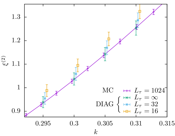
Figure 2: Correlation length $\xi^{(2)}$, see Eq. (34), versus $k$ as computed for $L=6$ lattices, both from Monte Carlo simulation on CPU and from exact diagonalization with EDQSG. The estimate from Monte Carlo simulation were obtained with Euclidean-time dimension $L_{\tau}=1024$, by averaging over 1280 samples (the continuous line is a cubic-spline interpolation). The results from exact diagonalization are an average over 320 samples ($L_{\tau}=\infty$ results are obtained from the eigenvector corresponding to the largest eigenvalue of the transfer matrix; the finite $L_{\tau}$ estimates are obtained by considering as well the eigenvector corresponding to the largest eigenvalue of the odd submatrix). To ease visualization, the data from exact diagonalization and $L_{\tau}=16$ and 32 were horizontally displaced by a constant amount.

We have carried out two important consistency checks for our main programs EDQSG and MCQSG.

In the case of EDQSG, we first computed $Q_{2}$, $Q_{4}$ and $F$ from a (standard CPU) Monte Carlo program on a lattice $L=4$ and $L=6$ and $L_{\tau}=1024$. This $L_{\tau}$ turns out to be big enough to allow a direct comparison with the outcome of EDQSG. Indeed, let $|GS\rangle$ be the eigenvector of the transfer matrix corresponding to its largest eigenvalue, and let

$$M_{\boldsymbol{x},\boldsymbol{y}} = \langle GS|\sigma^{Z}_{\boldsymbol{x}}\sigma^{Z}_{\boldsymbol{y}}|GS\rangle\,,$$ (30)

$$\tilde{M}_{\boldsymbol{x},\boldsymbol{y}} = \frac{1}{2}M_{\boldsymbol{x},\boldsymbol{y}}\Big{[}\cos\Big{(}\frac{2\pi}{L}(x_{1}-y_{1})\Big{)}+\cos\Big{(}\frac{2\pi}{L}(x_{2}-y_{2})\Big{)}\Big{]}\,,$$ (31)

$$R_{\boldsymbol{x},\boldsymbol{y},\boldsymbol{z},\boldsymbol{u}} = \langle GS|\sigma^{Z}_{\boldsymbol{x}}\sigma^{Z}_{\boldsymbol{y}}\sigma^{Z}_{\boldsymbol{z}}\sigma^{Z}_{\boldsymbol{u}}|GS\rangle\,,$$ (32)

Then, in the limit that concern us [2], namely $L_{\tau}\to\infty$, one has

$$Q_{2}=\text{Tr}M^{2}\,,\quad F=\text{Tr}M\tilde{M}\,,\quad Q_{4}=\sum_{\boldsymbol{x},\boldsymbol{y}\boldsymbol{z},\boldsymbol{u}}R^{2}_{\boldsymbol{x},\boldsymbol{y}\boldsymbol{z},\boldsymbol{u}}\,.$$ (33)

From them, one may compute the finite-lattice correlation length (see, e.g., Ref. [19])

$$\xi^{(2)}=\frac{1}{2\sin\frac{\pi}{L}}\sqrt{\frac{\overline{Q_{2}}}{\overline{F}}-1}\,$$ (34)

that we show in Figure 2 (the overlines indicate averages over samples). The figure carries two important messages. First, it shows that the limit $L_{\tau}\to\infty$ can be certainly reached within our numerical accuracy. And second, the Monte Carlo and Exact Diagonalization results are statistically compatible. Note that the results in Fig. 2 were obtained after averaging over samples. We have strengthened our test by comparing $Q_{2}$, $Q_{4}$ and $F$, as computed in the same sample with both approaches. Also at this finer level, statistical compatibility was found (at the $0.01\%$ level of accuracy reached in our Monte Carlo simulations).

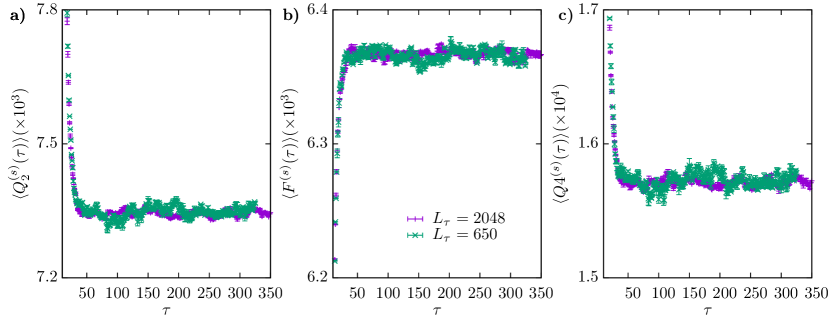
Figure 3: The time-correlation functions defined in Eqs. (27) (a),  (28) (b) and  (29) (c) versus $\tau$, as computed for the same sample from a standard CPU code $(L_{\tau}=650)$ and from the MCQSG program $(L_{\tau}=2048)$ at $k=0.29$ which is, approximately, the critical point for the model in Eq. (1), see Ref. [2].

As for the check of MCQSG, we have compared the time-correlation functions defined in Eqs. (27),  (28) and  (29) (c) with a standard CPU program on a lattice with $L=20$ and $L_{\tau}=650$. The same computation, on the same sample, has been carried out from the configurations produced by MCQSG on a lattice with $L=20$ and $L_{\tau}=2048$. The two computations are compared in Fig. 3. The statistical compatibility of the results at the plateaux, as well as the fact that the curves from the two programs reach their plateaux at the same $\tau$, is a most reasurring (and significant) check of overall consistency.

References

- [1] N. Hatano, M. Suzuki, “Finding Exponential Product Formulas of Higher Orders”. Quantum Annealing and Other Optimization Methods. Berlin, Heidelberg: Springer Berlin Heidelberg. pp. 37–68 (2005).
- [2] M. Bernaschi, I. González-Adalid Pemartín, V. Martín-Mayor, G. Parisi, “The Quantum Transition of the Two-Dimensional Ising Spin Glass: A Tale of Two Gaps”, arXiv:2310.07486 (2023).
- [3] https://petsc.org/
- [4] https://slepc.upv.es/
- [5] M. Bernaschi, M. Fatica, G. Parisi, L. Parisi, “Multi-GPU codes for spin systems simulations”, Computer Physics Communications 183, 1416, 2012.
- [6] L. Jacobs, C. Rebbi,“Multi-spin coding: A very efficient technique for Monte Carlo simulations of spin systems”, Journal of Computational Physics, Vol. 41, No. 1 (1981).
- [7] T. Preis, P. Virnau, W. Paul, J. J. Schneider, “GPU accelerated Monte Carlo simulation of the 2D and 3D Ising model,” J. of Comp. Phys., Vol. 228, 4468 (2009).
- [8] A. Pagnani and G. Parisi, “Multisurface coding simulations of the restricted solid-on-solid model in four dimensions”, Phys.Rev. E, Vol. 87, 010102(R) (2013).
-
[9]
J. Kelling, G. Ódor and S. Gemming, “Bit-vectorized GPU implementation of a
stochastic cellular automaton model for surface growth,” 2016 IEEE 20th
Jubilee International Conference on Intelligent Engineering Systems (INES),
Budapest, Hungary, pp. 233-237,
https:/doi: 10.1109/INES.2016.7555127(2016). - [10] L. A. Fernández and V. Martín-Mayor, “Testing statics-dynamics equivalence at the spin-glass transition in three dimensions”, Phys. Rev. B, Vol. 91, 174202 (2015).
-
[11]
N. Ito and Y. Kanada,“Monte Carlo simulation of the Ising model and random number generation on the vector processor”, Proceedings SUPERCOMPUTING ’90,
https:/doi.org/10.1109/SUPERC.1990.130097(1990). - [12] K. Hukushima, and K. Nemoto, “Exchange Monte Carlo Method and Application to Spin Glass Simulations”, J. Phys. Soc. Japan, Vol. 65, 1604, 1996.
-
[13]
J. Salmon, M. Moraes, R. Dror and D.E. Shaw, “Parallel Random Numbers: As Easy as 1, 2, 3”, Proceedings of Supercomputing 2011,
https://doi.org/10.1145/2063384.2063405}(2011). - [14] D. Blackman, S. Vigna, “Scrambled linear pseudorandom number generators”, ACM Transactions on Mathematical Software Vol. 47, 1 (2021).
- [15] C. Lanczos, “An iteration method for the solution of the eigenvalue problem of linear differential and integral operators”, United States Governm. Press Office Los Angeles, CA, 1950.
-
[16]
M. Baity-Jesi et al., “Janus II: a new generation
application-driven computer for spin-system simulations”,
Comp. Phys. Comm., Vol. 185, 550, 2014
(
https://doi.org/10.1016/j.cpc.2013.10.019). -
[17]
L.A. Fernandez, V. Martín-Mayor, S. Perez-Gaviro,
A. Tarancon and A. P. Young, “Phase transition in the three dimensional
Heisenberg spin glass: Finite-size scaling analysis”, Phys. Rev. B, Vol
80, 024422, 2009 (
https://doi.org/10.1103/PhysRevB.80.024422). -
[18]
A. Billoire et al., “Dynamic variational study of
chaos: spin glasses in three dimensions”, Journal of Statistical
Mechanics: Theory and Experiment, Vol. 2018, 33302, 2018 (
https://doi.org/10.1088/1742-5468/aaa387). -
[19]
D. J. Amit and V. Martín-Mayor, Field Theory, the
Renormalization Group and Critical Phenomena, World Scientific,
https://doi.org/10.1142/9789812775313_bmatter(2005).