Sensing Mutual Information with Random Signals in Gaussian Channels: Bridging Sensing and Communication Metrics

Abstract

Sensing performance is typically evaluated by classical radar metrics, such as Cramér-Rao bound and signal-to-clutter-plus-noise ratio. The recent development of the integrated sensing and communication (ISAC) framework motivated the efforts to unify the performance metric for sensing and communication, where mutual information (MI) was proposed as a sensing performance metric with deterministic signals. However, the need of communication in ISAC systems necessitates the transmission of random signals for sensing applications, whereas an explicit evaluation for the sensing mutual information (SMI) with random signals is not yet available in the literature. This paper aims to fill the research gap and investigate the unification of sensing and communication performance metrics. For that purpose, we first derive the explicit expression for the SMI with random signals utilizing random matrix theory. On top of that, we further build up the connections between SMI and traditional sensing metrics, such as ergodic minimum mean square error (EMMSE), ergodic linear minimum mean square error (ELMMSE), and ergodic Bayesian Cramér-Rao bound (EBCRB). Such connections open up the opportunity to unify sensing and communication performance metrics, which facilitates the analysis and design for ISAC systems. Finally, SMI is utilized to optimize the precoder for both sensing-only and ISAC applications. Simulation results validate the accuracy of the theoretical results and the effectiveness of the proposed precoding designs.

I Introduction

With the development of innovative applications that demand accurate environmental information, e.g., autonomous driving and unmanned aerial vehicle (UAV) networks, sensing becomes an essential requirement for future wireless networks. To this end, the integrated sensing and communications (ISAC) framework has attracted tremendous attention [2, 3, 4, 5, 6]. However, there are still substantial challenges that need to be tackled before we can fully unleash the potential of ISAC. One of the most significant issues is the distinct performance evaluation metrics for sensing and communication. In particular, sensing performance is typically characterized by metrics such as Cramér-Rao bound (CRB) [7], signal-to-clutter-plus-noise ratio [8], and minimum mean-square error (MMSE) [9], while communication performance is usually evaluated by the achievable rate [10], bit error rate [11], and outage probability [12]. The inconsistency in performance metrics between two systems poses challenges to the design of ISAC systems.

Recently, some research efforts have been devoted to unifying the performance metrics for sensing and communication. For that purpose, mutual information (MI), a metric commonly used to measure communication performance, has also been utilized to evaluate sensing performance [13, 14, 15]. The authors of [13] demonstrated that the waveform that maximizes the MI between the random target response and the received signal can also lead to enhanced sensing performance. The authors of [15] showed that the radar waveform that maximizes the MI between the Gaussian-distributed target response and the received signal also minimizes the MMSE for estimating the target response.

However, existing works [13, 14, 15] mainly focused on sensing mutual information (SMI) with deterministic signals, which have been widely employed in sensing applications, due to some favorable properties: 1) deterministic signals allow for precise control of key parameters, such as amplitude and phase of waveform, which enables accurate parameter estimation. For example, the radar using frequency modulated continuous wave (FMCW) can provide accurate range and velocity information [16, 17]; and 2) deterministic signals facilitate some important techniques in radar systems, such as pulse compression and coherent integration, which enhance range resolution and target detection ability [18, 19].

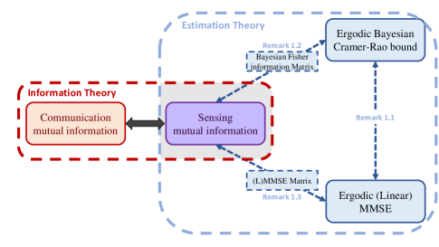
Figure 1: Illustration of the connection between SMI and other communication/sensing metrics.

In contrast to radar systems, communication applications require the signals to be random. As a result, it is crucial to evaluate the sensing performance with random signals in ISAC systems [20, 21, 22, 23, 24, 25]. However, the explicit evaluation for SMI with random signals remains widely unexplored, and in fact, even the evaluation for traditional sensing metrics with random signals is also missing. To this end, some researchers resorted to approximations or numerical methods [22, 23, 24, 25]. For example, the authors of [22] derived both lower and upper bounds for the Bayesian CRB with random signals, namely, the ergodic Bayesian CRB (EBCRB). In [24, 25], the ergodic linear MMSE (ELMMSE), which characterizes the estimation error of the target response matrix averaged over random signals, was studied for sensing system.

This paper aims to unify the performance metrics for sensing and communication in ISAC systems. For that purpose, we first derive an explicit expression for the SMI between the random target response and the received signals with random transmitting signals. It is shown that SMI can be interpreted as the maximum information that can be exacted from the target response matrix by the sensing receiver. Next, by studying the relation between SMI and other traditional sensing metrics, e.g., ergodic MMSE (EMMSE), ELMMSE, and EBCRB, we demonstrate that SMI can serve as a bridge to connect communication and sensing metrics, as illustrated in Fig. 1. One interesting finding is that SMI is directly related to Bayesian Fisher information and maximizing SMI is equivalent to minimizing the EBCRB, which is the lower bound for the estimation error of Bayesian estimators. Moreover, the estimation error of MMSE and LMMSE estimators approaches the BCRB in the case that the target response matrix is Gaussian-distributed.

The connections between SMI and traditional sensing metrics, along with the widespread use of MI in measuring the performance of communication systems, motivate us to adopt MI for evaluating the communication and sensing performance in a unified manner. To demonstrate the benefits of such a unified framework, we investigate the precoding designs for both sensing-only and ISAC applications, by imposing MI as the performance metric. Simulations results show that the proposed methods achieve superior performance than existing methods.

The main contributions of this paper are summarized as:

1. We derive explicit expressions for SMI, EMMSE, ELMMSE, and EBCRB with random signals by leveraging random matrix theory. It is shown that the SMI with random signals is upper-bounded by that with a properly-designed deterministic signal. Furthermore, as the number of samples increases, the SMI loss caused by the utilization of random signals will diminish.

2. We demonstrate that SMI can serve as a bridge to connect communication and sensing metrics. In particular, we build up the connections between SMI, EMMSE, ELMMSE, and EBCRB. These results provide a unified framework for evaluating communication and sensing performance, facilitating the analysis and design of ISAC systems.

3. Building upon the theoretical results, we propose two precoding design methods for sensing-only and ISAC scenarios. Remarkably, although a fixed-point equation is involved in the computation of SMI, the explicit expression for its gradient is available, which enables efficient optimization. Simulation results validate the accuracy of the theoretical analysis results and effectiveness of the proposed optimization methods.

The remainder of the paper is organized as follows. Section II presents the system model. Section III provides an explicit expression for the SMI and reveals some physical insights. Section IV studies the relation between SMI and other sensing metrics and provides a physical interpretation for SMI. Section V introduces two approaches to maximize the SMI by optimizing the transmitted precoder for both sensing-only and ISAC systems. Simulation results are given in Section VI to validate the accuracy of the theoretical results and the effectiveness of the proposed optimization-based approaches. Finally, Section VII concludes the paper, summarizing the key findings and contributions.

II System Model

Consider an ISAC system composed of an ISAC transmitter with $N_{T}$ antennas, a communication receiver with $N_{C}$ antennas, and a sensing receiver with $N_{R}$ antennas as shown in Fig. 2. In this paper, we consider the simultaneous downlink transmission and target sensing with the bi-static sensing scheme. In the following, we will present the communication and sensing model, respectively.

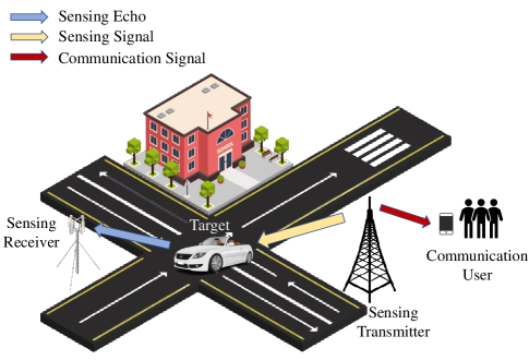
Figure 2: Illustration of the considered ISAC system.

II-A Communication model

The received communication signal is given by

$$\begin{split}\mathbf{Y}_{c}=\mathbf{H}_{c}\mathbf{X}+\mathbf{N}_{c}\in\mathbb{C}^{N_{C}\times N_{S}},\end{split}$$ (1)

where $\mathbf{X}\in\mathbb{C}^{N_{T}\times N_{S}}$ represents the transmitted signal, $\mathbf{H}_{c}\in\mathbb{C}^{N_{C}\times N_{T}}$ denotes the MIMO communication channel, and $\mathbf{N}_{c}$ represents the additive white Gaussian noise. In this paper, we consider the widely adopted Gaussian signal with $\mathbf{X}=\mathbf{F}\mathbf{S}$, where $\mathbf{F}\in\mathbb{C}^{N_{T}\times N_{T}}$ represents the precoding matrix and $\mathbf{S}\in\mathbb{C}^{N_{T}\times N_{S}}$ denotes a random matrix whose entries are independent and identically distributed (i.i.d.) Gaussian random variables with variance $\frac{1}{N_{S}}$ and $N_{S}\geq N_{T}$. It follows that $\mathbb{E}(\mathbf{S}\mathbf{S}^{\mathrm{H}})=\mathbf{I}$. The communication performance can be measured by the MI between the received and transmitted signals, i.e.,

$$\begin{split}I_{c}&=I(\mathbf{Y}_{c};\mathbf{S}|\mathbf{H}_{c})=\log\left|\mathbf{I}+\sigma_{c}^{2}\mathbf{H}_{c}\mathbf{F}\mathbf{F}^{\mathrm{H}}\mathbf{H}_{c}^{\mathrm{H}}\right|.\end{split}$$ (2)

II-B Sensing model

The objective for sensing is to estimate the parameters of interest (POI) of targets based on the received signals, with the knowledge of the transmitted probing signal. Assume that the target sensing is performed within a coherent processing interval (CPI) consisting of $N_{S}$ frames. The baseband signal received by the sensing receiver in a CPI is given by [14]

$$\begin{split}\mathbf{Y}_{s}=\mathbf{H}_{s}\mathbf{X}+\mathbf{N}_{s}\in\mathbb{C}^{N_{R}\times N_{S}},\end{split}$$ (3)

where $\mathbf{H}_{s}$ represents the target response matrix, and $\mathbf{N}_{s}\in\mathbb{C}^{N_{R}\times N_{S}}$ is the additive white Gaussian noise. In this paper, we assume $\mathbf{X}$ is random but known to the sensing receiver.

By stacking the columns of $\mathbf{Y}_{s}^{\mathrm{H}}$, we can obtain

$$\begin{split}\mathbf{y}_{s}\triangleq\text{vec}(\mathbf{Y}_{s}^{\mathrm{H}})=\left(\mathbf{I}_{N_{R}}\otimes\mathbf{X}\right)^{\mathrm{H}}\mathbf{h}_{s}+\mathbf{n}_{s}\in\mathbb{C}^{N\times 1},\end{split}$$ (4)

where $N=N_{T}N_{R}$, $\mathbf{h}_{s}=\text{vec}(\mathbf{H}_{s}^{\mathrm{H}})$, and $\mathbf{n}_{s}=\text{vec}(\mathbf{N}_{s}^{\mathrm{H}})\sim\mathcal{CN}(\mathbf{0},\sigma_{s}^{2}\mathbf{I}_{N})$. The correlation matrix $\mathbf{R}\triangleq\mathbb{E}(\mathbf{h}_{s}\mathbf{h}_{s}^{\mathrm{H}})$ is given by $\mathbf{R}=\mathbf{R}_{R}\otimes\mathbf{R}_{T}$ [26, 27, 28], where $\mathbf{R}_{R}$ and $\mathbf{R}_{T}$ denote the correlation matrices at the receiver and the transmitter, respectively. Note that $\mathrm{rank}(\mathbf{R}_{R})\leq K$ and $\mathrm{rank}(\mathbf{R}_{T})\leq K$, where $K$ denotes the number of sensing targets. In this paper, we assume $\mathbf{R}_{R}$ and $\mathbf{R}_{T}$ are available to the transmitter. This assumption is justified in ISAC systems, where the prior knowledge of the targets can be obtained from previous estimation [9, 14].

For target detection, the sensing receiver shall estimate the target response vector $\mathbf{h}_{s}$ based on the received signals $\mathbf{y}_{s}$, or $\mathbf{H}_{s}$ based on $\mathbf{Y}_{s}$, equivalently [14, 29]. Assuming a deterministic sensing signal, previous works focused on the system design by optimizing $\mathbf{S}$ to maximize the sensing mutual information (SMI) between the received signals and the target response [14, 15]. Unfortunately, such methods are no longer valid for ISAC systems when random signals are utilized. To this end, we will evaluate the SMI with random signals in the next section.

III Sensing Mutual Information with Random Signals

In this section, we derive an explicit expression for the SMI with random signals by employing random matrix theory. Based on this derived expression, we will study the influence of $N_{S}$ and investigate the relation between SMI and other sensing performance metrics, such as the ELMMSE and EBCRB.

Define $\bm{\eta}$ as the POI of the targets, e.g., AOA, AOD and reflection coefficients. We assume that $\bm{\eta}$ remains constant in one CPI and varies between CPIs in an i.i.d. manner. Any estimator for $\bm{\eta}$ aims to estimate a particular realization of $\bm{\eta}$ within one CPI. When $\mathbf{H}_{s}$ is an injective map of $\bm{\eta}$, the MI between $\bm{\eta}$ and the received signals $\mathbf{y}_{s}$ is equivalent to that between $\mathbf{h}_{s}$ and $\mathbf{y}_{s}$, i.e., $I\left(\bm{\eta};\mathbf{y}_{s}|\mathbf{S}\right)=I\left(\mathbf{h}_{s};\mathbf{y}_{s}|\mathbf{S}\right)$ [20].

For ease of evaluation, we assume that $\mathbf{h}_{s}$ follows a Gaussian distribution, i.e., $\mathbf{h}_{s}\sim\mathcal{CN}(\mathbf{0},\mathbf{R})$, which has been widely adopted for MIMO channel [27] and target response matrix [14, 15, 20]. Under such circumstances, the SMI with random signals is defined as [20]

$$\begin{split}&I_{s}=I\left(\mathbf{h}_{s};\mathbf{y}_{s}|\mathbf{S}\right)\\ &\triangleq\mathbb{E}_{\mathbf{S}}\log\left|\mathbf{I}+\sigma_{s}^{-2}\left(\mathbf{R}_{R}\otimes\mathbf{R}_{T}^{\frac{1}{2}}\mathbf{F}\mathbf{S}\mathbf{S}^{\mathrm{H}}\mathbf{F}^{\mathrm{H}}\mathbf{R}_{T}^{\frac{1}{2}}\right)\right|,\end{split}$$ (5)

where the expectation is taken over the random signals $\mathbf{S}$. According to [20], SMI is directly related to the distortion metric (e.g., the estimation error) of $\bm{\eta}$. Unfortunately, the expectation in (5) is computationally prohibitive due to the high-dimensional integrals.

III-A Upper bound of SMI

An upper bound of SMI can be obtained by applying the Jensen’s inequality on (5). In particular, we have

$$\begin{split}I_{s}\leq\log\left|\mathbf{I}+\sigma_{s}^{-2}\left(\mathbf{R}_{R}\otimes\mathbf{R}_{T}^{\frac{1}{2}}\mathbf{F}\mathbb{E}_{\mathbf{S}}(\mathbf{S}\mathbf{S}^{\mathrm{H}})\mathbf{F}^{\mathrm{H}}\mathbf{R}_{T}^{\frac{1}{2}}\right)\right|,\end{split}$$ (6)

where the equality holds when $\mathbf{S}\mathbf{S}^{\mathrm{H}}=\mathbf{I}$. Accordingly, we can obtain the upper bound as

$$\begin{split}&I_{s,\max}\triangleq\log\left|\mathbf{I}+\sigma_{s}^{-2}\left(\mathbf{R}_{R}\otimes\mathbf{R}_{T}^{\frac{1}{2}}\mathbf{\Phi}\mathbf{R}_{T}^{\frac{1}{2}}\right)\right|,\\ \end{split}$$ (7)

where $\mathbf{\Phi}=\mathbf{F}\mathbf{F}^{\mathrm{H}}$. Thus, there are two ways to interpret $I_{s,\max}$. On the one hand, $I_{s,\max}$ can be regarded as the MI obtained by a deterministic signal $\mathbf{S}$ with $\mathbf{S}\mathbf{S}^{\mathrm{H}}=\mathbf{I}$. On the other hand, as an upper bound, $I_{s,\max}$ can be utilized as an approximation for SMI when $N_{S}$ is large. This is because, as $N_{S}\to\infty$, the sample covariance matrix $\mathbf{S}\mathbf{S}^{\mathrm{H}}$ will tend to be deterministic, i.e., $\lim_{N_{S}\to\infty}\mathbf{S}\mathbf{S}^{\mathrm{H}}\to\mathbf{I}$. Under such circumstances, $I_{s}$ approaches its upper bound $I_{s,\max}$. Unfortunately, as we will show later, the precision of this approximation is poor when $N_{S}$ is small.

III-B Asymptotic approximation of SMI

In this paper, we derive an explicit expression for the SMI by analyzing the asymptotic behavior of $I\left(\mathbf{h}_{s};\mathbf{y}_{s}\right)$. In particular, we provide an approximation for the SMI in the large $N_{S}$ regime based on the first order approximation of the MI. The result is shown in the following proposition.

Proposition 1

As $N_{S},N_{T}\to\infty$ with a finite constant ratio $c$, i.e., $N_{S}/N_{T}=c$, we have

$$\begin{split}I_{s}=\sum_{j=1}^{K}\bar{\varrho}_{j}(\mathbf{\Phi})+\mathcal{O}\left(\frac{1}{N_{S}}\right),\end{split}$$ (8)

where

$$\begin{split}&\bar{\varrho}_{j}(\mathbf{\Phi})=\log\left|\mathbf{I}_{N_{T}}+\frac{\lambda_{R,j}}{1+\lambda_{R,j}\delta(\lambda_{R,j})}\mathbf{T}(\mathbf{\Phi})\right|\\ &+N_{S}\log(1+\lambda_{R,j}\delta(\lambda_{R,j}))-N_{S}\frac{\lambda_{R,j}\delta(\lambda_{R,j})}{1+\lambda_{R,j}\delta(\lambda_{R,j})},\end{split}$$ (9)

with

$$\mathbf{T}(\mathbf{\Phi})\triangleq\mathbf{R}_{T}^{\frac{1}{2}}\mathbf{\Phi}\mathbf{R}_{T}^{\frac{1}{2}}.$$ (10)

$\{\lambda_{R,j}\}_{j=1}^{K}$ denotes the eigenvalues of $\sigma_{s}^{-2}\mathbf{R}_{R}$, and $\delta(\rho)$ is the solution to the following equation

$$\delta(\rho)=\frac{1}{N_{S}}\mathrm{tr}\left(\mathbf{T}(\mathbf{\Phi})\left(\mathbf{I}_{N_{T}}+\frac{\rho}{1+\rho\delta(\rho)}\mathbf{T}(\mathbf{\Phi})\right)^{-1}\right).$$ (11)

Proof: See Appendix A. $\blacksquare$

Proposition 1 provides an explicit expression for the SMI between the POI and the received signals. Note that, different from the upper bound in (7), Proposition 1 aims to approximate SMI by analyzing its asymptotic behavior. As will be shown later, although (8) is derived under the condition that $N_{S}$ and $N_{T}$ approach infinity, it provides accurate approximation for the SMI even when $N_{S}$ and $N_{T}$ are small.

III-C Effect of the number of frames

With the explicit expression of the SMI, we can analyze the impact of key system parameters. To evaluate the effect of $N_{S}$, we calculate the derivative of the SMI with respect to $N_{S}$. For all $N_{S}\geq 0$, the derivative of $\bar{\varrho}_{j}(\mathbf{\Phi})$, which is given in (9), with respect to $N_{S}$ can be expressed in the form of

$$\frac{\partial\bar{\varrho}_{j}}{\partial N_{S}}=-\frac{\lambda_{R,j}^{2}\mathrm{tr}\left[\mathbf{T}\left(\mathbf{I}_{N_{T}}+\frac{\lambda_{R,j}}{1+\lambda_{R,j}\delta(\lambda_{R,j})}\mathbf{T}\right)^{-1}\right]}{(1+\lambda_{R,j}\delta(\lambda_{R,j}))^{2}}\cdot\frac{\partial\delta(\lambda_{R,j})}{\partial N_{S}}$$

$$\quad+\left(\frac{N_{S}\lambda_{R,j}}{1+\lambda_{R,j}\delta(\lambda_{R,j})}-\frac{N_{S}\lambda_{R,j}}{(1+\lambda_{R,j}\delta(\lambda_{R,j}))^{2}}\right)\cdot\frac{\partial\delta(\lambda_{R,j})}{\partial N_{S}}$$

$$\quad+\log(1+\lambda_{R,j}\delta(\lambda_{R,j}))-\frac{\lambda_{R,j}\delta(\lambda_{R,j})}{1+\lambda_{R,j}\delta(\lambda_{R,j})}$$ (12)

$$\overset{(a)}{=}\log(1+\lambda_{R,j}\delta(\lambda_{R,j}))-\frac{\lambda_{R,j}\delta(\lambda_{R,j})}{1+\lambda_{R,j}\delta(\lambda_{R,j})}\geq 0,$$

where step (a) follows (11). Thus, we have

$$\frac{\partial I_{s}}{\partial N_{S}}=\sum_{j=1}^{K}\frac{\partial\bar{\varrho}_{j}}{\partial N_{S}}\geq 0.$$ (13)

This indicates that the SMI $I_{s}$ is monotonically increasing with respect to $N_{S}$.

III-D Sensing DoF loss

To measure the impact of random signals on sensing, we further investigate the sensing Degree of Freedom (DoF). This concept was introduced in [22] to measure the loss of CRB induced by the random signals and defined as the effective number of independent observations. By following the same idea, we define the SMI-oriented sensing DoF as

$$\nu_{s}=\lim_{\sigma_{s}^{2}\to 0}N_{S}\frac{I_{s}}{I_{s,\max}}.$$ (14)

where the maximum sensing DoF is the total number of the independent observations $N_{S}$. The normalization coefficient $\frac{I_{s}}{I_{s,\max}}$ is the ratio between the SMI with random signals and its upper bound achieved by deterministic signals. Thus, this ratio measures the MI loss caused by the randomness of signals. The following proposition provides the lower bound for $I\left(\bm{\eta};\mathbf{y}_{s}|\mathbf{S}\right)$, based on which the maximum sensing DoF loss can be obtained.

Proposition 2

When $N_{S}\geq N_{T}$, we have

$$\begin{split}\!\!I_{s}\geq\frac{N_{S}-\min\{K,\mathrm{rank}(\mathbf{\Phi})\}}{N_{S}}I_{s,\max}.\end{split}$$ (15)

Proof: See Appendix C. $\blacksquare$

Based on Proposition 2, the sensing DoF can be bounded by

$$N_{S}-\min\{K,\mathrm{rank}(\mathbf{\Phi})\}\leq\nu_{s}\leq N_{S}.$$ (16)

This indicates that $\min\{K,\mathrm{rank}(\mathbf{\Phi})\}$ is the maximum sensing DoF loss defined based on SMI, which coincides with that defined based on CRB [22]. It can be observed that the maximum sensing DoF loss will increase with $K$. This is because the system needs to separate the signals associated with different targets, and this task becomes more challenging as the number of targets increases, due to the interference among different targets. As a result, more samples are required to mitigate such a loss. In particular, according to the squeeze theorem, there is no loss when $N_{S}\to\infty$, because the lower bound of $I_{s}$ in (15) approaches $I_{s,\max}$. This agrees with the theoretical results in (13).

IV Relation between SMI and Other Sensing Performance Metrics

Section III investigated SMI but the operational meaning of SMI remains unclear [20]. In particular, for communication, MI has a clear operational meaning and is directly related to the achievable data rate. However, for sensing, the information of the concerned physical parameters is “encoded” and “transmitted” through the target response matrix to the receiver in a passive manner, and the MI between the target response matrix and the received signal does not bear any direct physical meaning.

To fill in this gap, we will investigate the relation between SMI and other sensing performance metrics, e.g., sensing ELMMSE and Bayesian CRB. By examining these connections, we aim to shed light on the unification of the performance metrics for communication and sensing. For that purpose, we first evaluate the EMMSE, ELMMSE, and Bayesian CRB with random signals.

IV-A ELMMSE and EMMSE for estimating $\mathbf{h}_{s}$

To evaluate the average sensing performance with random signals, the ergodic linear minimum mean square error (ELMMSE) was investigated in [24]. The ELMMSE for estimating $\mathbf{h}_{s}$ is given by

$$\begin{split}J_{\mathrm{ELMMSE}}&=\mathbb{E}_{\mathbf{S}}[\mathrm{tr}(\mathbf{\Psi}_{\mathrm{LMMSE}}(\mathbf{S}))],\end{split}$$ (17)

where

$$\begin{split}\mathbf{\Psi}_{\mathrm{LMMSE}}(\mathbf{S})&\triangleq\mathbb{E}[(\hat{\mathbf{h}}_{s,\text{LMMSE}}-\mathbf{h}_{s})(\hat{\mathbf{h}}_{s,\text{LMMSE}}-\mathbf{h}_{s})^{\mathrm{H}}],\end{split}$$ (18)

denotes the data-dependent LMMSE matrix with $\hat{\mathbf{h}}_{s,\text{LMMSE}}$ representing the LMMSE estimate of $\mathbf{h}_{s}$. For a Gaussian-distributed $\mathbf{h}_{s}$, we have

$$\begin{split}\mathbf{\Psi}_{\mathrm{LMMSE}}(\mathbf{S})=\mathbf{R}\left(\mathbf{I}+\sigma_{s}^{-2}\left(\mathbf{R}_{R}\otimes\mathbf{R}_{T}^{\frac{1}{2}}\mathbf{F}\mathbf{S}\mathbf{S}^{\mathrm{H}}\mathbf{F}^{\mathrm{H}}\mathbf{R}_{T}^{\frac{1}{2}}\right)\right)^{-1}.\end{split}$$ (19)

A lower bound for sensing ELMMSE can be obtained by applying the Jensen’s inequality on (17), i.e.,

$$\begin{split}J_{\mathrm{ELMMSE}}\geq\mathrm{tr}\left[\mathbf{R}\left(\mathbf{I}+\sigma_{s}^{-2}\left(\mathbf{R}_{R}\otimes\mathbf{R}_{T}^{\frac{1}{2}}\mathbf{\Phi}\mathbf{R}_{T}^{\frac{1}{2}}\right)\right)^{-1}\right].\end{split}$$ (20)

However, an explicit expression for the sensing ELMMSE is not yet available in the literature. In the following, we derive an explicit expression for the sensing ELMMSE by analyzing its asymptotic approximation in the following proposition.

Proposition 3

As $N_{S},N_{T}\to\infty$ with a finite constant ratio $c$, i.e., $N_{S}/N_{T}=c$, we have

$$\begin{split}&J_{\mathrm{ELMMSE}}=\sum_{j=1}^{K}\bar{\varkappa}_{j}(\mathbf{\Phi})+\mathcal{O}\left(\frac{1}{N_{S}}\right),\end{split}$$ (21)

where

$$\begin{split}\bar{\varkappa}_{j}(\mathbf{\Phi})=\sigma_{s}^{2}\lambda_{R,j}\mathrm{tr}\left(\mathbf{R}_{T}\mathbf{M}_{T,j}\right),\end{split}$$ (22)

with

$$\begin{split}\mathbf{M}_{T,j}=\left(\mathbf{I}_{N_{T}}+\frac{\lambda_{R,j}}{1+\lambda_{R,j}\delta(\lambda_{R,j})}\mathbf{T}(\mathbf{\Phi})\right)^{-1}.\end{split}$$ (23)

Proof: See Appendix D.

Proposition 3 provides an explicit expression for the ELMMSE of estimating $\mathbf{h}_{s}$ by analyzing its asymptotic behavior. As will be shown later, (21) is more accurate than the lower bound in (20), even when $N_{S}$ and $N_{T}$ are small.

To evaluate the effect of $N_{S}$, we calculate the derivative for the ELMMSE with respect to $N_{S}$. For all $N_{S}\geq 0$, we have

$$\begin{split}\frac{\partial\delta(\lambda_{R,j})}{\partial N_{S}}=&-\frac{1}{N_{S}^{2}}\mathrm{tr}\left(\mathbf{T}\mathbf{M}_{T,j}\right)\\ &+\frac{\alpha(\lambda_{R,j})^{2}\mathrm{tr}\left(\mathbf{M}_{T,j}\mathbf{T}\right)^{2}}{N_{S}}\cdot\frac{\partial\delta(\lambda_{R,j})}{\partial N_{S}},\end{split}$$ (24)

where

$$\begin{split}\alpha(\rho)=\frac{\rho}{1+\rho\delta(\rho)}.\end{split}$$ (25)

By solving the linear equation (24), we have

$$\begin{split}\frac{\partial\delta(\lambda_{R,j})}{\partial N_{S}}=\frac{-\delta(\lambda_{R,j})}{N_{S}-\alpha(\lambda_{R,j})^{2}\mathrm{tr}\left(\mathbf{T}\mathbf{M}_{T,j}\right)^{2}}.\end{split}$$ (26)

Since $\alpha(\lambda_{R,j})\geq 0$, we can obtain

$$\alpha(\lambda_{R,j})^{2}\mathrm{tr}\left(\mathbf{T}\mathbf{M}_{T,j}\right)^{2}=\mathrm{tr}\left(\mathbf{T}\left(\alpha^{-1}(\lambda_{R,j})\mathbf{I}+\mathbf{T}\right)^{-1}\right)^{2}$$

$$=\sum_{i=1}^{N_{T}}\left(\frac{\lambda_{T,i}}{\alpha^{-1}(\lambda_{R,j})+\lambda_{T,i}}\right)^{2}\leq\mathrm{rank}(\mathbf{T})\leq N_{S}.$$ (27)

Thus, we have $\frac{\partial\delta(\lambda_{R,j})}{\partial N_{S}}\leq 0.$ The derivative of $\bar{\varkappa}_{j}(\mathbf{\Phi})$ with respect to $N_{S}$ can then be given by

$$\begin{split}\frac{\partial\bar{\varkappa}_{j}(\mathbf{\Phi})}{\partial N_{S}}=\alpha(\lambda_{R,j})^{2}\mathrm{tr}\left(\mathbf{M}_{T,j}\mathbf{R}_{T}\mathbf{M}_{T,j}\mathbf{T}\right)\frac{\partial\delta(\lambda_{R,j})}{\partial N_{S}}.\end{split}$$ (28)

Since $\alpha(\lambda_{R,j})^{2}\mathrm{tr}\left(\mathbf{M}_{T,j}\mathbf{R}_{T}\mathbf{M}_{T,j}\mathbf{T}\right)\geq 0$, we have

$$\begin{split}\frac{\partial J_{\mathrm{ELMMSE}}}{\partial N_{S}}=\sum_{j=1}^{K}\frac{\partial\bar{\varkappa}_{j}(\mathbf{\Phi})}{\partial N_{S}}\leq 0.\end{split}$$ (29)

This indicates that the sensing ELMMSE $J_{\mathrm{ELMMSE}}$ is monotonically decreasing with respect to $N_{S}$.

Given $\mathbf{S}$, the MMSE matrix for estimating $\mathbf{h}_{s}$ is defined as

$$\mathbf{\Psi}_{\mathrm{MMSE}}(\mathbf{S})=\mathbb{E}[(\mathbf{h}_{s}-\mathbb{E}(\mathbf{h}_{s}|\mathbf{y}_{s}))(\mathbf{h}_{s}-\mathbb{E}(\mathbf{h}_{s}|\mathbf{y}_{s}))^{\mathrm{H}}].$$ (30)

For a Gaussian distributed $\mathbf{h}_{s}$, the MMSE estimator is identical to the LMMSE estimator. Therefore, we can also define the EMMSE as $J_{\mathrm{EMMSE}}=J_{\mathrm{ELMMSE}}$.

IV-B Ergodic Bayesian CRB for estimating $\mathbf{h}_{s}$

The Bayesian CRB provides a lower bound for the MSE of unbiased Bayesian estimators. Different from the conventional CRB, the Bayesian CRB takes the prior information regarding the channel $\mathbf{h}_{s}$ into account. Based on the model defined in (4), the Bayesian Fisher information matrix for estimating $\mathbf{h}_{s}$ is given by [22]

$$\mathbf{J}\triangleq\mathbb{E}\left(\frac{\partial p_{\mathbf{h}_{s}}(\mathbf{h}_{s})}{\partial\mathbf{h}_{s}}\frac{\partial p_{\mathbf{h}_{s}}(\mathbf{h}_{s})}{\partial\mathbf{h}_{s}^{\mathrm{H}}}\right)$$ (31)

$$+\mathbb{E}\left(\left.\frac{\partial\log p_{\mathbf{y}_{s}|\mathbf{S},\mathbf{h}_{s}}(\mathbf{y}_{s}|\mathbf{S},\mathbf{h}_{s})}{\partial\mathbf{h}_{s}}\frac{\partial\log p_{\mathbf{y}_{s}|\mathbf{S},\mathbf{h}_{s}}(\mathbf{y}_{s}|\mathbf{S},\mathbf{h}_{s})}{\partial\mathbf{h}_{s}^{\mathrm{H}}}\right|\mathbf{S}\right).$$

For a Gaussian-distributed $\mathbf{h}_{s}$, the BCRB matrix is defined as the inverse of the Bayesian Fisher information matrix, i.e.,

$$\begin{split}\mathbf{\Psi}_{\mathrm{BCRB}}(\mathbf{S})\triangleq\mathbf{J}^{-1}=\left(\mathbf{R}^{-1}+\sigma_{s}^{-2}\mathbf{I}_{N_{R}}\otimes\mathbf{X}\mathbf{X}^{\mathrm{H}}\right)^{-1}.\\ \end{split}$$ (32)

To evaluate the sensing performance, specific functions of the BCRB matrix are normally adopted as the metric of sensing performance, e.g., the determinant [30] and the trace [31]. Hence, we can give the explicit expressions for two forms of EBCRB with random signals based on Proposition 1 and Proposition 3 as

$$\mathrm{EBCRB}_{1}\triangleq\mathbb{E}_{\mathbf{S}}\log|\mathbf{\Psi}_{\mathrm{BCRB}}(\mathbf{S})|\approx\sum_{j=1}^{K}\bar{\varrho}_{j}(\mathbf{\Phi}),$$ (33)

$$\mathrm{EBCRB}_{2}\triangleq\mathbb{E}_{\mathbf{S}}\mathrm{tr}(\mathbf{\Psi}_{\mathrm{BCRB}}(\mathbf{S}))\approx\sum_{j=1}^{K}\bar{\varkappa}_{j}(\mathbf{\Phi}).$$ (34)

IV-C Relation between different metrics

For estimating a Gaussian-distributed $\mathbf{h}_{s}$, the following proposition reveals the relations between SMI, EBCRB, EMMSE, and ELMMSE.

Proposition 4

For a Gaussian-distributed $\mathbf{h}_{s}$, the SMI $I\left(\mathbf{h}_{s};\mathbf{y}_{s}|\mathbf{S}\right)$ defined in (5), the MMSE matrix $\mathbf{\Psi}_{\mathrm{MMSE}}$ defined in (30), the LMMSE matrix $\mathbf{\Psi}_{\mathrm{LMMSE}}$ defined in (19), and the BCRB matrix $\mathbf{\Psi}_{\mathrm{BCRB}}$ defined in (32) have the following relation

$$\begin{split}\mathbf{\Psi}_{\mathrm{BCRB}}(\mathbf{S})=\mathbf{\Psi}_{\mathrm{MMSE}}(\mathbf{S})=\mathbf{\Psi}_{\mathrm{LMMSE}}(\mathbf{S}),\end{split}$$ (35)

and

$$\begin{split}I\left(\mathbf{h}_{s};\mathbf{y}_{s}|\mathbf{S}\right)=\log|\mathbf{R}|-\mathbb{E}_{\mathbf{S}}\log|\mathbf{\Psi}_{\mathrm{BCRB}}(\mathbf{S})|.\end{split}$$ (36)

Proof: Recalling from (19) and (32), we have $\mathbf{\Psi}_{\mathrm{BCRB}}=\mathbf{\Psi}_{\mathrm{LMMSE}}$. Then, according to the squeeze theorem, recalling (42), we can obtain that $\mathbf{\Psi}_{\mathrm{BCRB}}=\mathbf{\Psi}_{\mathrm{MMSE}}=\mathbf{\Psi}_{\mathrm{LMMSE}}$.

Recalling (33), we have

$$\begin{split}&\log|\mathbf{\Psi}_{\mathrm{BCRB}}(\mathbf{S})|\\ &=\log|\mathbf{R}|-\log\left|\mathbf{I}+\sigma_{s}^{-2}\left(\mathbf{R}_{R}\otimes\mathbf{R}_{T}^{\frac{1}{2}}\mathbf{F}\mathbf{S}\mathbf{S}^{\mathrm{H}}\mathbf{F}^{\mathrm{H}}\mathbf{R}_{T}^{\frac{1}{2}}\right)\right|.\end{split}$$ (37)

By taking the expectation with respect to $\mathbf{S}$ on both sides of (37) and recalling (5), we have

$$\begin{split}\mathbb{E}_{\mathbf{S}}\log|\mathbf{\Psi}_{\mathrm{BCRB}}(\mathbf{S})|=\log|\mathbf{R}|-I\left(\mathbf{h}_{s};\mathbf{y}_{s}|\mathbf{S}\right),\end{split}$$ (38)

which completes the proof. $\blacksquare$

According to the definition of MI, we have

$$I\left(\mathbf{h}_{s};\mathbf{y}_{s}|\mathbf{S}\right)=H(\mathbf{h}_{s}|\mathbf{S})-H(\mathbf{h}_{s}|\mathbf{y}_{s},\mathbf{S}),$$ (39)

where $H(\cdot)$ denotes the entropy operator. Since the target response matrix $\mathbf{h}_{s}$ follows the Gaussian distribution $\mathcal{CN}(\mathbf{0},\mathbf{R})$ and is independent of $\mathbf{S}$, we have $H(\mathbf{h}_{s}|\mathbf{S})=H(\mathbf{h}_{s})=\log|\mathbf{R}|.$ Then, we have

$$H(\mathbf{h}_{s}|\mathbf{y}_{s},\mathbf{S})=\log|\mathbf{R}|-I\left(\mathbf{h}_{s};\mathbf{y}_{s}|\mathbf{S}\right).$$ (40)

It follows from (19) that

$$\begin{split}H(\mathbf{h}_{s}|\mathbf{y}_{s},\mathbf{S})=\mathbb{E}_{\mathbf{S}}\log|\mathbf{\Psi}_{\mathrm{BCRB}}(\mathbf{S})|.\end{split}$$ (41)

Remark 1

Proposition 4 reveals some insights:

1. EBCRB vs EMMSE/ELMMSE (the connection labeled as Remark 1.1 in Fig. 1): For the Gaussian-distributed $\mathbf{h}_{s}$, we know that, the BCRB matrix is identical to the LMMSE and MMSE matrix, i.e., $\mathbf{\Psi}_{\mathrm{BCRB}}(\mathbf{S})=\mathbf{\Psi}_{\mathrm{MMSE}}(\mathbf{S})=\mathbf{\Psi}_{\mathrm{LMMSE}}(\mathbf{S})$. This indicates that the estimation error of MMSE and LMMSE estimator can approach BCRB.

2. SMI vs EBCRB (the connection labeled as Remark 1.2 in Fig. 1): The equation $I\left(\mathbf{h}_{s};\mathbf{y}_{s}|\mathbf{S}\right)=\log|\mathbf{R}|-\mathbb{E}_{\mathbf{S}}\log|\mathbf{\Psi}_{\mathrm{BCRB}}(\mathbf{S})|$ indicates that SMI is directly related to Bayesian Fisher information as $\mathbf{\Psi}_{\mathrm{BCRB}}=\mathbf{J}^{-1}$.

   This equivalence offers an interesting connection between information theory and estimation theory. In particular, wireless sensing can be interpreted as “non-cooperative” communication, where the target plays the role of a non-cooperative transmitter, which encodes information about the POI $\bm{\eta}$ into the target response matrix $\mathbf{h}_{s}$ and transmits $\mathbf{h}_{s}$ to the sensing receiver. Here, we use $H(\mathbf{h}_{s})=\log|\mathbf{R}|$ to represent the uncertainty about the target response $\mathbf{h}_{s}$. Then, the sensing receiver will decode this information to estimate the POI based on the echoes $\mathbf{y}_{s}$, where $H(\mathbf{h}_{s}|\mathbf{y}_{s},\mathbf{S})$ denotes the uncertain about $\mathbf{h}_{s}$ when $\mathbf{y}_{s}$ is known.

   The mutual information $I\left(\mathbf{h}_{s};\mathbf{y}_{s}|\mathbf{S}\right)=H(\mathbf{h}_{s}|\mathbf{S})-H(\mathbf{h}_{s}|\mathbf{y}_{s},\mathbf{S})$ is the reduction of the uncertainty about $\mathbf{h}_{s}$, when $\mathbf{y}_{s}$ is observed. From the perspective of estimation theory, the utilization of certain estimators to recover POI from $\mathbf{y}_{s}$ inevitably introduces estimation errors. The MSE of Bayesian estimators with random signals is lower-bounded by the EBCRB, i.e., $\mathbb{E}_{\mathbf{S}}\log|\mathbf{\Psi}_{\mathrm{BCRB}}(\mathbf{S})|$. The equality $\mathbb{E}_{\mathbf{S}}\log|\mathbf{\Psi}_{\mathrm{BCRB}}(\mathbf{S})|=H(\mathbf{h}_{s}|\mathbf{y}_{s},\mathbf{S})$ indicates that such inevitable errors are identical to the uncertainty of $\mathbf{h}_{s}$ when $\mathbf{y}_{s}$ is observed, which comes from the noise or ill-conditioned channel. In other words, the SMI $I\left(\mathbf{h}_{s};\mathbf{y}_{s}|\mathbf{S}\right)$ can be interpreted as the maximum amount of information about $\mathbf{h}_{s}$ that can be extracted by Bayesian estimators.

3. SMI vs EMMSE/ELMMSE (the connection labeled as Remark 1.3 in Fig. 1): From Proposition 4, we have $I\left(\mathbf{h}_{s};\mathbf{y}_{s}|\mathbf{S}\right)=\log|\mathbf{R}|-\mathbb{E}_{\mathbf{S}}\log|\mathbf{\Psi}_{\mathrm{MMSE}}(\mathbf{S})|$. Given the log-determinant of MMSE matrix has also been widely used to represent MMSE [32], we can see that SMI is directly related to EMMSE and ELMMSE.

The aforementioned connections between SMI and traditional sensing metrics, e.g., EBCRB, EMMSE, and ELMMSE, highlight the effectiveness of SMI as a metric for evaluating sensing performance. Given MI has been widely utilized to evaluate communication performance, we propose to leverage MI as a unified metric for both sensing and communication.

When $\mathbf{h}_{s}$ is non-Gaussian distributed, the relation between SMI and other sensing metrics is different. In particular, with a deterministic signal $\mathbf{S}$, the relation between BCRB, MMSE and LMMSE is given by [33]

$$\mathbf{\Psi}_{\mathrm{BCRB}}(\mathbf{S})\preceq\mathbf{\Psi}_{\mathrm{MMSE}}(\mathbf{S})\preceq\mathbf{\Psi}_{\mathrm{LMMSE}}(\mathbf{S}),$$ (42)

which indicates that, the MMSE is a lower bound of LMMSE. This is because the LMMSE estimator is obtained by minimizing the MSE within linear estimators. Meanwhile, BCRB is a lower bound for the estimation error of Bayesian estimators, including both MMSE and LMMSE estimators. Moreover, given any realization of $\mathbf{S}$, i.e., $\mathbf{S}=\mathbf{A}$, the relation between BCRB and MI is given by [33]

$$I\left(\mathbf{h}_{s};\mathbf{y}_{s}|\mathbf{S}=\mathbf{A}\right)\geq-\log|\mathbf{\Psi}_{\mathrm{BCRB}}(\mathbf{A})|-\log|\mathbf{J}_{X}|,$$ (43)

where

$$\mathbf{J}_{X}\triangleq\mathbb{E}\left(\frac{\partial p_{\mathbf{h}_{s}}(\mathbf{h}_{s})}{\partial\mathbf{h}_{s}}\frac{\partial p_{\mathbf{h}_{s}}(\mathbf{h}_{s})}{\partial\mathbf{h}_{s}^{\mathrm{H}}}\right).$$ (44)

By taking expectation over $\mathbf{A}$ on both sides of (43), we have

$$I\left(\mathbf{h}_{s};\mathbf{y}_{s}|\mathbf{S}\right)\geq-\mathbb{E}_{\mathbf{A}}\log|\mathbf{\Psi}_{\mathrm{BCRB}}(\mathbf{A})|-\log|\mathbf{J}_{X}|.$$ (45)

Nevertheless, the explicit expressions of these sensing metrics for estimating a non-Gaussian $\mathbf{h}_{s}$ with random signals are not yet available, and will be left as a future research direction.

V SMI-Oriented Precoding Design

In this section, we will optimize the precoder to maximize the SMI for sensing-only and ISAC scenarios, respectively. In particular, given SMI serves as an effective metric for evaluating sensing performance, we maximize the SMI under a constraint on the transmit power in the sensing-only scenario. In the ISAC scenario, besides the transmit power constraint, we also introduce one constraint on the communication MI. By doing this, we aim to demonstrate that MI can serve as a unified metric for ISAC.

V-A Sensing-only scenario

For sensing-only systems, the optimization problem is formulated as

$$\begin{array}[]{ccl}&\min\limits_{\mathbf{\Phi}\in\mathcal{A}}&\mathcal{L}_{s}(\mathbf{\Phi}),\\ \end{array}$$ (46)

where

$$\mathcal{L}_{s}(\mathbf{\Phi})=-I\left(\bm{\eta};\mathbf{y}_{s}|\mathbf{S}\right),$$ (47)

and $\mathcal{A}=\{\mathbf{\Phi}\in\mathbb{C}^{N_{T}\times N_{T}}|\mathbf{\Phi}=\mathbf{\Phi}^{\mathrm{H}},\mathrm{tr}(\mathbf{\Phi})\leq P\}$ denotes the feasible region, which indicates that the transmit power is constrained by a maximum value of $P$. A common practice to solve (46) is to utilize the interior point method associated with the Newton’s method, which requires both gradient and Hessian matrix. However, since $\delta$ is obtained by solving the equation defined in (11), it is difficult to obtain the Hessian matrix of $\mathcal{L}_{s}(\mathbf{\Phi})$ with respect to $\mathbf{\Phi}$. To address this issue, we propose to solve the problem in (46) by exploiting the gradient-projection (GP) method, which makes it easier to deal with the constraint and only requires the gradient.

Define $\nabla_{\mathbf{\Phi}}\mathcal{L}_{s}(\mathbf{\Phi})$ as the gradient of the objective function in (46) with respect to $\mathbf{\Phi}$. Note that $\delta$ defined in (11) is dependent on $\mathbf{\Phi}$, which makes the derivative more complex. To this end, we first obtain the derivatives of $\delta(\rho)$ with respect to $\mathbf{\Phi}$by the following lemma.

Lemma 1

Define $\alpha(\rho)=\frac{\rho}{1+\rho\delta(\rho)}$. Then, the gradient of $\delta(\rho)$ with respect to $\mathbf{\Phi}$, i.e., $\mathbf{\Delta}_{\rho}^{\prime}\triangleq\frac{\partial\delta(\rho)}{\partial\mathbf{\Phi}^{*}}$ is obtained by

$$\begin{split}&\mathbf{\Delta}_{\rho}^{\prime}=\frac{\mathbf{R}_{T}^{\frac{1}{2}}\left(\mathbf{I}+\alpha(\rho)\mathbf{T}(\mathbf{\Phi})\right)^{-2}\mathbf{R}_{T}^{\frac{1}{2}}}{N_{S}-\alpha^{2}(\rho)\mathrm{tr}(\mathbf{T}(\mathbf{\Phi})\left(\mathbf{I}+\alpha(\rho)\mathbf{T}(\mathbf{\Phi})\right)^{-1})^{2}}.\end{split}$$ (48)

Proof: See Appendix B. $\blacksquare$

It is interesting to observe that, although $\delta$ should be obtained by a fixed-point equation, the explicit expression of its gradient is available.

Then, the gradient of $\bar{\varrho}_{j}(\mathbf{\Phi})$ with respect to $\mathbf{\Phi}$ is given in the following proposition.

Proposition 5

The gradient of $\bar{\varrho}_{j}(\mathbf{\Phi})$ with respect to $\mathbf{\Phi}$ is given by

$$\nabla_{\mathbf{\Phi}}\bar{\varrho}_{j}(\mathbf{\Phi})\triangleq\frac{\partial\bar{\varrho}_{j}(\mathbf{\Phi})}{\partial\mathbf{\Phi}^{*}}=\alpha_{j}\mathbf{R}_{T}^{\frac{1}{2}}\mathbf{M}_{T,j}\mathbf{R}_{T}^{\frac{1}{2}}.$$ (49)

Proof: See Appendix E. $\blacksquare$

Corollary 1

The gradient of $\bar{\varkappa}_{j}(\mathbf{\Phi})$ with respect to $\mathbf{\Phi}$ is given by

$$\begin{split}&\nabla_{\mathbf{\Phi}}\bar{\varkappa}_{j}(\mathbf{\Phi})\triangleq\frac{\partial\bar{\varkappa}_{j}(\mathbf{\Phi})}{\partial\mathbf{\Phi}^{*}}\\ &=\sigma_{s}^{2}\lambda_{R,j}\alpha_{j}^{2}\mathrm{tr}\left(\mathbf{R}_{T}\mathbf{M}_{T,j}\mathbf{T}\mathbf{M}_{T,j}\right)\mathbf{\Delta}_{\lambda_{R,j}}^{\prime}(\mathbf{\Phi})\\ &\quad-\sigma_{s}^{2}\lambda_{R,j}\alpha_{j}\mathbf{R}_{T}^{\frac{1}{2}}\mathbf{M}_{T,j}\mathbf{R}_{T}\mathbf{M}_{T,j}\mathbf{R}_{T}^{\frac{1}{2}},\end{split}$$ (50)

where

$$\mathbf{\Delta}_{\lambda_{R,j}}^{\prime}(\mathbf{\Phi})=\mathbf{\Delta}_{\rho}^{\prime}|_{\rho=\lambda_{R,j}}.$$ (51)

Proof: See Appendix F. $\blacksquare$

Therefore, $\nabla_{\mathbf{\Phi}}\mathcal{L}_{s}(\mathbf{\Phi})$ is computed as

$$\begin{split}\nabla_{\mathbf{\Phi}}\mathcal{L}_{s}(\mathbf{\Phi})=-\sum_{j=1}^{K}\nabla_{\mathbf{\Phi}}\bar{\varrho}_{j}(\mathbf{\Phi}),\end{split}$$ (52)

where $\nabla_{\mathbf{\Phi}}\bar{\varrho}_{j}(\mathbf{\Phi})$ is defined in (49).

Then, at the $m$th iteration, $\mathbf{\Phi}^{(m+1)}$ is updated by

$$\begin{split}&\widehat{\mathbf{\Phi}}^{(m+1)}=\mathbf{\Phi}^{(m)}-\beta_{m}\nabla_{\mathbf{\Phi}}\mathcal{L}_{s}(\mathbf{\Phi}^{(m)}),\end{split}$$ (53)

where $\beta_{m}$ denotes the step size obtained via the Armijo line search [34, Definition 4.2.2]. A projection is needed to remap the updated points onto the feasible region. The projection of $\mathcal{A}$ is defined as

$$\mathbf{\Phi}^{(m+1)}=\mathcal{F}\left(\widehat{\mathbf{\Phi}}^{(m+1)}\right),$$ (54)

where

$$\begin{split}\mathcal{F}(\mathbf{\Phi})=\left\{\begin{array}[]{lcl}&\mathbf{\Phi},&\mathrm{if\;}\mathbf{\Phi}\in\mathcal{A}\\ &\frac{P}{\mathrm{tr}(\mathbf{\Phi})}\mathbf{\Phi},&\mathrm{otherwise}\end{array}\right..\end{split}$$ (55)

The convergence of the proposed GP-based method is guaranteed by [35].

V-B ISAC scenario

Next, we will optimize the precoder to maximize the SMI for ISAC system while guaranteeing the communication performance. The optimization problem is formulated as

$$\begin{array}[]{ccl}&\min\limits_{\mathbf{\Phi}\in\mathcal{A}}&\mathcal{L}_{s}(\mathbf{\Phi})\\ &s.t.&I_{c}(\mathbf{\Phi})\geq R_{0},\end{array}$$ (56)

where $I_{c}(\mathbf{\Phi})$ denotes the communication data rate, which is defined in (2). The main difference between (56) and (46) is the constraint where $R_{0}$ denotes a required level of communication performance. Note that the expression of $\mathcal{L}_{s}(\mathbf{\Phi})$ is complex with respect to $\mathbf{\Phi}$. Therefore, although both the cost function and the constraints are convex, (56) is hard to solve directly. To this end, we exploit the ADMM by introducing an auxiliary variable $\mathbf{\Omega}$, such that $\eqref{P0}$ can be recast as

$$\begin{array}[]{ccl}\mathcal{P}_{1}:&\min\limits_{\mathbf{\Phi},\mathbf{\Omega}\in\mathcal{A}}&\mathcal{L}_{s}(\mathbf{\Phi})\\ &s.t.&I_{c}(\mathbf{\Omega})\geq R_{0},\quad\mathbf{\Omega}=\mathbf{\Phi}.\end{array}$$ (57)

The problem (57) leads to the augmented Lagrangian function

$$\mathcal{L}(\mathbf{\Phi},\mathbf{\Omega},\mathbf{\Delta})=\mathcal{L}_{s}(\mathbf{\Phi})+\frac{\rho}{2}\left\|\mathbf{\Phi}-\mathbf{\Omega}+\mathbf{\Delta}\right\|^{2},$$ (58)

where $\rho$ is a penalty parameter. Then, at the $m$th iteration, the variables can be updated as

$$\mathbf{\mathbf{\Phi}}^{(m+1)}=\arg\min_{\mathbf{\mathbf{\Phi}}\in\mathcal{A}}\mathcal{L}(\mathbf{\Phi},\mathbf{\Omega}^{(m)},\mathbf{\Delta}^{(m)}),$$ (59a)

$$\mathbf{\Omega}^{(m+1)}=\arg\min_{\mathbf{\Omega}\in\mathcal{A}}\mathcal{L}(\mathbf{\Phi}^{(m+1)},\mathbf{\Omega},\mathbf{\Delta}^{(m)}),$$ (59b)

$$\quad\quad\quad\quad\quad\text{s.t.}\;I_{c}(\mathbf{\Omega})\geq R_{0},$$

$$\mathbf{\Delta}^{(m+1)}=\mathbf{\Delta}^{(m)}+\mathbf{\mathbf{\Phi}}^{(m+1)}-\mathbf{\Omega}^{(m+1)},$$ (59c)

where $\mathbf{\mathbf{\Phi}}^{(m+1)}$, $\mathbf{\Omega}^{(m)}$, and $\mathbf{\Delta}^{(m)}$ denotes $\mathbf{\Phi}$, $\mathbf{\Omega}$, and $\mathbf{\Delta}$ at the $m$th iteration, respectively.

V-B1 Update $\mathbf{\mathbf{\Phi}}^{(m+1)}$ via (59a)

Since (59a) resembles (46), we propose to solve (59a) by a GP-based method similar to the proposed method in the sensing-only scenario. The gradient of $\mathcal{L}(\mathbf{\Phi}|\mathbf{\Omega}^{(m)},\mathbf{\Delta}^{(m)})$ with respect to $\mathbf{\Phi}$ is

$$\begin{split}&\nabla_{\mathbf{\Phi}}\mathcal{L}(\mathbf{\Phi}|\mathbf{\Omega}^{(m)},\mathbf{\Delta}^{(m)})\\ &=-\sum_{j=1}^{K}\nabla_{\mathbf{\Phi}}\bar{\varrho}_{j}(\mathbf{\Phi})+\rho\left(\mathbf{\mathbf{\Phi}}-\mathbf{\Omega}^{(m)}+\mathbf{\Delta}^{(m)}\right)^{\mathrm{H}}\mathbf{\mathbf{\Phi}}.\end{split}$$ (60)

Then, $\mathbf{\Phi}^{(m+1)}$ is updated by

$$\begin{split}&\mathbf{\Phi}^{(m+1)}=\mathbf{\Phi}^{(m)}-\beta_{m}\nabla_{\mathbf{\Phi}}\mathcal{L}(\mathbf{\Phi}^{(m)}).\end{split}$$ (61)

V-B2 Update $\mathbf{\Omega}^{(m+1)}$ via (59b)

The resultant problem (59b) is equivalent to

$$\begin{split}\min_{\mathbf{\Omega}\in\mathcal{A}}\;&\left\|\mathbf{\Phi}^{(m+1)}-\mathbf{\Omega}+\mathbf{\Delta}^{(m)}\right\|^{2}\\ s.t.\;&I_{c}(\mathbf{\Omega})\geq R_{0}.\end{split}$$ (62)

This problem is a typical semi-definite programming (SDP) problem because the objective function and all constraints are reformulated as a linear or quadratic form. This problem can be easily solved by the CVX toolbox [36].

The cost function will not increase over the ADMM iteration process given in (59). According to the monotone bounded theorem [37], the iteration will converge to a set of stationary points in the feasible set.

VI Simulation Results

In this section, we will validate the accuracy of the theoretical analysis and the effectiveness of proposed optimization-based algorithms by simulation. We consider a mmWave system operating at a carrier frequency of 28 GHz [38]. The AOD and AOA of the targets are generated uniformly in the range $[30^{\circ},60^{\circ}]$. The number of antennas at the transmitter and receiver is set as $N_{T}=16$ and $N_{R}=16$, respectively. For the GP-based optimization, we set the maximum number of iterations as $40$. To terminate the iteration, the tolerance for the norm of the gradient between two iterations is set as $10^{-10}$. The transmission power is set as $P=30$ dBm, the noise power is $\sigma^{2}=-90$ dBm, and the SNR at the sensing receiver is 10 dB, unless otherwise specified.

VI-A Validation of the theoretical results

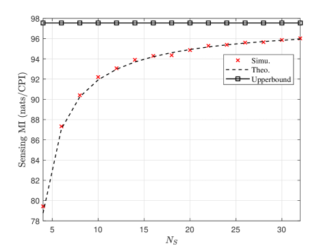
Figure 3: Sensing MI versus the number of frames $N_{S}$.

SMI: Fig. 3 validates the accuracy of the evaluation for SMI in Proposition 1 with $K=7$ targets. The legend ‘Simu.’ denotes the MI obtained by Monte-Carlo simulations, i.e.,

$$\begin{split}\bar{I}\left(\bm{\eta};\mathbf{y}_{s}|\mathbf{S}\right)=\frac{1}{N_{mc}}\sum_{i=1}^{N_{mc}}I\left(\bm{\eta};\mathbf{y}_{s}|\mathbf{S}=\mathbf{S}_{i}\right),\end{split}$$

where $\mathbf{S}_{i}$ denotes the $i$th realization of $\mathbf{S}$ and $N_{mc}=5000$ represents the number of Monte-Carlo trails. The legend ‘Theo.’ denotes the theoretical result of the SMI given in (8). The legend ‘Upperbound’ denotes the upper bound in (7) and the legend ‘Lowerbound’ represents the lower bound of SMI given in Proposition 2. Although Proposition 1 indicates that $I\left(\bm{\eta};\mathbf{y}_{s}|\mathbf{S}\right)$ will approach $\sum_{j=1}^{K}\bar{\varrho}_{j}(\mathbf{\Phi})$ as $N_{S}$ goes to infinity, it can be observed that the approximation in (7) is very accurate, even when $N_{S}$ is small. This observation validates the accuracy of Proposition 1. Meanwhile, a discrepancy consistently exists between SMI and its upper bound, which is more obvious when $N_{S}$ is small.

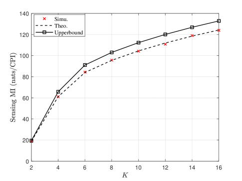
Figure 4: Sensing MI versus the number of targets $K$.

Fig. 4 compares the theoretical and simulation results with respect to the number of targets $K$, where we set $N_{S}=8$. We can observe that SMI will increase with $K$. This is because with more targets, there is more information to be estimated. However, it is important to note that as $K$ increases, the discrepancy between SMI and its upper bound becomes more pronounced. As discussed in Sec. III. D, this is due to the increase in the sensing DoF loss. Sensing DoF represents the effective number of independent measurements that can be obtained from the observed data. As $K$ increases, more targets introduce more constraints and dependencies among the measurements, resulting in a larger loss of sensing DoF. Therefore, more samples are required to approach the upper bound of SMI, potentially leading to high latency. Moreover, it is important to note that the relationship between $K$ and SMI is not linear. The increase in SMI with $K$ tends to saturate at a larger $K$, because there is a limit on the amount of information that can be extracted from a given number of samples.

Figure 5: Normalized ELMMSE versus the number of frames $N_{S}$.

ELMMSE: Fig. 5 validates the accuracy of the evaluation for ELMMSE in Proposition 3 with $K=7$ targets. The normalized ELMMSE is defined as

$$\bar{\varepsilon}_{M}=\frac{J_{\mathrm{ELMMSE}}}{\mathbb{E}\;\|\mathbf{h}_{s}\|^{2}}=\frac{J_{\mathrm{ELMMSE}}}{\mathrm{tr}(\mathbf{R})}.$$

The legend ‘Lowerbound’ denotes the lower bound in (20). It can be observed that the approximation in (21) is accurate, particularly when $N_{S}$ is large, which validates Proposition 3. With a larger number of samples, the exact value of ELMMSE converges towards its lower bound.

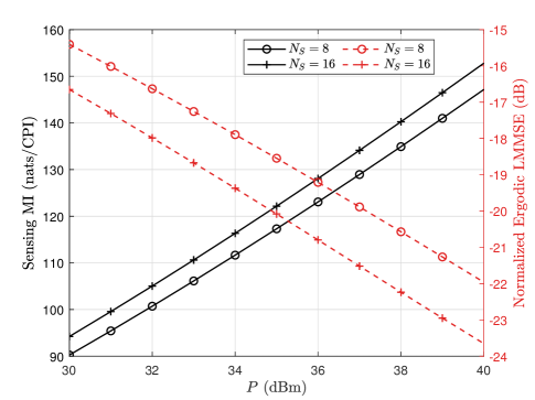
Figure 6: Sensing MI and normalized ELMMSE versus $P$.

Validation of Proposition 4: Fig. 6 compares SMI and the normalized ELMMSE with different values of $P$. From Fig. 6, we can observe that as $P$ increases, the SMI increases while the normalized ELMMSE decreases. For example, when $P=30$ dBm and $N_{S}=8$, SMI is about $90.1$ nats/CPI and the normalized ELMMSE is about $-15.3$ dB. When $P=36$ dBm and $N_{S}=8$, SMI is about $123.2$ nats/CPI and the normalized ELMMSE is about $-19.1$ dB. This observation agrees with Proposition 4.

VI-B Precoding design for sensing

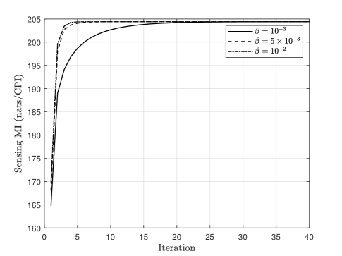
Figure 7: Convergence performance of the proposed GP-based sensing precoding design method.

Convergence: Fig. 7 demonstrates the convergence behavior of the proposed GP-based method, where the number of frames is set as $N_{S}=8$. We set the step size as $\beta_{m}=10^{-3},5\times 10^{-3}$, and $10^{-2}$, respectively. Note that the convergence speed can be affected by $\beta_{m}$. From Fig. 7, we can observe that the proposed GP-based method can converge after several iterations for different values of $\beta_{m}$. Therefore, further exploration of different $\beta_{m}$ may be necessary to improve the convergence speed and reach the desired solution. This search can be done through techniques such as grid search or adaptive methods that dynamically adjust the value of $\beta_{m}$ during the optimization process.

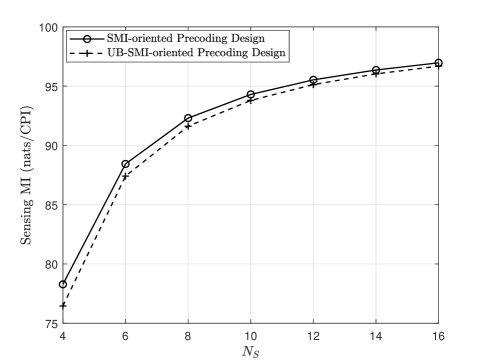
Figure 8: Sensing MI versus $N_{S}$.

Effect of $N_{S}$: Note that, as $N_{S}\to\infty$, SMI will approach its upper bound (7). This allows us to utilize the upper bound as an approximation when $N_{S}$ is large. The SMI as a function of $N_{S}$ is shown in Fig. 8, where the legend ‘SMI-oriented Precoding Design’ denotes the SMI obtained by the method that maximizes the SMI in (8) and the legend ‘UB-SMI-oriented Precoding Design’ represents the SMI obtained by the method that maximizes (7). It can be observed that the proposed method which maximizes the SMI outperforms the one maximizing its upperbound, and the performance gap between the two methods becomes smaller as $N_{S}$ increases. This can be attributed to the fact that the mismatch between the SMI and its upper bound diminishes as $N_{S}$ increases.

Effect of transmit power $P_{0}$: Next, we investigate the impact of transmit power on the optimization results. It can be observed from Fig. 9 that SMI will increase with the SNR, achieving a more reliable and accurate estimation of the POIs. This is because SMI represents the amount of information that can be extracted from the observed data regarding POIs. With a higher SNR, the observed data is less corrupted by noise, allowing for more precise estimation of the POIs.

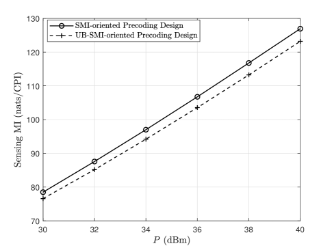
Figure 9: Sensing MI versus $P_{0}$ ($N_{S}=4$).

VI-C Precoding design for ISAC

In this section, we will evaluate the performance of the proposed ADMM-based ISAC precoding design method. We consider a communication user equipped with $4$ antennas. The distance between the ISAC transmitter and communication receiver is set as $20$ m. The communication requirement is set as $R_{0}=20$ bps/Hz, the number of targets is $K=15$, the transmit power is $P_{0}=30$ dBm, the penalty parameter is $\rho=10^{4}$, and the optimization step size is $\beta_{m}=1.5\times 10^{-4}$.

Convergence: We begin with the convergence performance of the proposed ADMM-based ISAC precoding design method. Since SMI is a function of $\mathbf{\Phi}$, we denote $\mathcal{F}_{s}(\mathbf{\Phi})=I\left(\bm{\eta};\mathbf{y}_{s}|\mathbf{S}\right)$. Fig. 10 shows the SMI with respect to the dual variables $\mathbf{\Phi}$ and $\mathbf{\Omega}$ over the ADMM iterations, i.e., $\mathcal{F}_{s}(\mathbf{\Phi})$ and $\mathcal{F}_{s}(\mathbf{\Omega})$, respectively. We can observe from Fig. 10 that the proposed algorithm can converge within about 50 iterations.

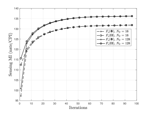
Figure 10: Convergence performance of the proposed ADMM-based ISAC precoding design method.

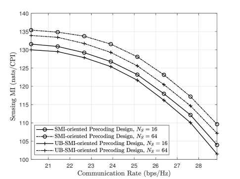
Figure 11: Sensing and Communication tradeoff under different precoding schemes.

Tradeoff between sensing and communication: Next, we will show the performance tradeoff between sensing and communication in Fig. 11. To this end, MI is utilized as a unified metric for evaluating both sensing and communication performance. Specifically, the communication MI is used as a performance metric for communication, while SMI serves as a performance metric for sensing. From Fig. 11, we can observe that as the communication rate increases, the SMI will decrease. This is because there is an inherent competition between sensing and communication in an ISAC system. Additionally, the results obtained by optimizing the SMI surpass those obtained by optimizing its upper bound in (7).

VII Conclusion

This paper contributed to the unification of sensing and communication performance metrics. For that purpose, we started by deriving an explicit expression for SMI with random signals using random matrix theory. Based on these results, we established the connections between SMI, EMMSE, ELMMSE, and EBCRB. These connections demonstrated that SMI can serve as a bridge to connect communication and sensing metrics, providing a unified framework for the analysis and design of ISAC systems. Finally, two optimization-based methods were proposed to maximize the SMI by designing the precoder for both sensing-only and ISAC scenarios. Simulation results validated the accuracy of the theoretical results and the effectiveness of the proposed optimization-based methods.

Appendix A Proof of Proposition 1

This proof is equivalent to analyze the asymptotic behavior of the following random variable

$$\begin{split}\varrho=\log\left|\mathbf{I}+\sigma_{s}^{-2}\mathbf{R}_{R}\otimes(\mathbf{R}_{T}^{\frac{1}{2}}\mathbf{F}\mathbf{S}\mathbf{S}^{\mathrm{H}}\mathbf{F}^{\mathrm{H}}\mathbf{R}_{T}^{\frac{1}{2}})\right|.\end{split}$$ (63)

In fact, Proposition 1 is an extension of [10, Theorems 1], which is summarized in the following lemma.

Lemma 2 ([10, Theorems 1])

Given two deterministic diagonal matrices $\mathbf{D}\in\mathcal{R}^{N\times N}$ and $\widetilde{\mathbf{D}}\in\mathcal{R}^{n\times n}$, we can define $\mathbf{Z}=\mathbf{D}^{\frac{1}{2}}\widetilde{\mathbf{Z}}\widetilde{\mathbf{D}}^{\frac{1}{2}}$, where $\widetilde{\mathbf{Z}}$ has i.i.d. entries following complex Gaussian distribution $\mathcal{CN}(0,\frac{1}{n})$. Then, we have

$$\begin{split}\mathbb{E}\log\left|\rho\mathbf{Z}\mathbf{Z}^{\mathrm{H}}+\mathbf{I}\right|=V_{n}(\rho)+\mathcal{O}\left(\frac{1}{n}\right),\end{split}$$ (64)

where

$$\begin{split}V_{n}(\rho)=&\log\left|\mathbf{I}+\rho\delta(\rho)\widetilde{\mathbf{D}}\right|+\log\left|\mathbf{I}+\rho\tilde{\delta}(\rho)\mathbf{D}\right|-n\rho\delta(\rho)\tilde{\delta}(\rho),\end{split}$$

and $(\delta(\rho),\tilde{\delta}(\rho))$ is the unique positive solution of the following fixed-point equations

$$\begin{split}\left\{\begin{matrix}\delta=\frac{1}{n}\mathrm{tr}\left(\mathbf{D}\left(\mathbf{I}+\rho\tilde{\delta}\mathbf{D}\right)^{-1}\right)\\ \tilde{\delta}=\frac{1}{n}\mathrm{tr}\left(\widetilde{\mathbf{D}}\left(\mathbf{I}+\rho\delta\widetilde{\mathbf{D}}\right)^{-1}\right)\end{matrix}\right..\end{split}$$ (65)

The main idea of this proof is to recast $I\left(\mathbf{h}_{s};\mathbf{y}_{s}|\mathbf{S}\right)$ into an extended model which fits into the framework of [10].

First, by utilizing the property of block diagonal matrix and the equality $\det(\mathbf{I}+\mathbf{A}\mathbf{B})=\det(\mathbf{I}+\mathbf{B}\mathbf{A})$, (63) can be rewritten as

$$\varrho=\sum_{j=1}^{K}\varrho_{j},$$ (66)

where

$$\varrho_{j}=\log\det\left(\mathbf{I}_{N_{T}}+\lambda_{R,j}\mathbf{R}_{T}^{\frac{1}{2}}\mathbf{F}\mathbf{S}\mathbf{S}^{\mathrm{H}}\mathbf{F}^{\mathrm{H}}\mathbf{R}_{T}^{\frac{1}{2}}\right).$$

By performing the eigenvalue decomposition on $\mathbf{R}_{T}^{\frac{1}{2}}\mathbf{F}$, we have $\mathbf{R}_{T}^{\frac{1}{2}}\mathbf{F}=\mathbf{U}_{T}\widetilde{\mathbf{\Lambda}}_{T,0}\mathbf{V}_{T}^{\mathrm{H}}$, where $\mathbf{U}_{T}\in\mathbb{C}^{N_{T}\times N_{T}}$ and $\mathbf{V}_{T}\in\mathbb{C}^{K\times K}$ denote the left- and right-singular vectors, respectively. Meanwhile, $\widetilde{\mathbf{\Lambda}}_{T}$ is a rectangular diagonal matrix with non-negative real numbers on the diagonal, i.e.,

$$\begin{split}\widetilde{\mathbf{\Lambda}}_{T,0}=\left[\begin{matrix}\mathbf{\Lambda}_{T}^{\frac{1}{2}}\\ \mathbf{0}\end{matrix}\right],\end{split}$$ (67)

with $\mathbf{\Lambda}_{T}\in\mathbb{C}^{K\times K}$ denotes the eigenvalue matrix of $\mathbf{T}\triangleq\mathbf{R}_{T}^{\frac{1}{2}}\mathbf{F}\mathbf{F}^{\mathrm{H}}\mathbf{R}_{T}^{\frac{1}{2}}$, i.e., $\mathbf{T}=\mathbf{U}_{T}\widetilde{\mathbf{\Lambda}}_{T}\mathbf{U}_{T}^{\mathrm{H}}$, where

$$\begin{split}\widetilde{\mathbf{\Lambda}}_{T}=\left[\begin{matrix}\mathbf{\Lambda}_{T}&\mathbf{0}\\ \mathbf{0}&\mathbf{0}\end{matrix}\right].\end{split}$$ (68)

Note that, with any unitary matrices $\mathbf{U}$ and $\mathbf{V}$, the random matrices $\mathbf{U}\mathbf{S}\mathbf{V}$ and $\mathbf{S}$ are statistically equivalent [10]. Thus, by omitting some constants independent of $\mathbf{S}$, the asymptotic behavior of $\varrho_{j}$ is equivalent to that of the RV

$$\hat{\varrho}_{j}=\log\det\left(\mathbf{I}_{K}+\lambda_{R,j}\mathbf{\Lambda}_{T}^{\frac{1}{2}}\mathbf{S}\mathbf{S}^{\mathrm{H}}\mathbf{\Lambda}_{T}^{\frac{1}{2}}\right).$$ (69)

By invoking $\mathbf{D}=\mathbf{\Lambda}_{T}$, $\widetilde{\mathbf{D}}=\mathbf{I}_{N_{S}}$, $n=N_{S}$, and $\rho=\lambda_{R,j}$ into (65), we have $\tilde{\delta}(\rho)=1/(1+\rho\delta)$ such that the fixed-point equations in (65) reduce to a linear one with respect to $\delta$, i.e.,

$$\delta(\rho)=\frac{1}{N_{S}}\mathrm{tr}\left(\mathbf{\Lambda_{T}}\left(\mathbf{I}_{K}+\frac{\rho}{1+\rho\delta(\rho)}\mathbf{\Lambda_{T}}\right)^{-1}\right).$$ (70)

Furthermore, from Lemma 1, we can obtain that, as $N_{S},N_{T}\to\infty$, one has

$$\begin{split}\mathbb{E}(\hat{\varrho}_{j})=\bar{\varrho}_{j}+\mathcal{O}\left(\frac{1}{N_{S}}\right),j=1,2,\cdots,\end{split}$$ (71)

where

$$\begin{split}&\bar{\varrho}_{j}=\log\left|\mathbf{I}_{K}+\frac{\lambda_{R,j}}{1+\lambda_{R,j}\delta(\lambda_{R,j})}\mathbf{\Lambda_{T}}\right|\\ &+N_{S}\log(1+\lambda_{R,j}\delta(\lambda_{R,j}))-\frac{N_{S}\lambda_{R,j}\delta(\lambda_{R,j})}{1+\lambda_{R,j}\delta(\lambda_{R,j})}.\end{split}$$ (72)

Then, by utilizing the property of the unitary matrix $\mathbf{U}_{T}$, (72) and (70) are equivalent to (9) and (11), respectively, which completes the proof.

Appendix B Proof of Lemma 1

From (11), we have $\delta(\rho)=\frac{1}{N_{S}}\mathrm{tr}(\mathbf{T}\mathbf{M}_{T}),$ where $\mathbf{M}_{T}(\rho)\triangleq\left(\mathbf{I}_{N_{S}}+\alpha(\rho)\mathbf{T}\right)^{-1}$ and $\alpha(\rho)=\frac{\rho}{1+\rho\delta(\rho)}$. The derivative of $\alpha(\rho)$ with respect to the $(m,n)$th entry of $\mathbf{F}$, denoted by $F_{m,n}^{*}$, is given by

$$\begin{split}\alpha_{m,n}^{\prime}(\rho)&=\frac{\partial\alpha(\rho)}{\partial\Phi_{m,n}^{*}}=-\alpha^{2}(\rho)[\mathbf{\Delta}_{\rho}^{\prime}(\mathbf{\Phi})]_{m,n}.\end{split}$$ (73)

The derivative of $\mathbf{T}$ with respect to $F_{m,n}^{*}$ can be expressed as

$$\begin{split}[{\mathbf{T}^{\prime}}]_{m,n}=\frac{\partial\mathbf{T}}{\partial\Phi_{m,n}^{*}}=\mathbf{R}_{T}^{\frac{1}{2}}\mathbf{e}_{n}\mathbf{e}_{m}^{\mathrm{T}}\mathbf{R}_{T}^{\frac{1}{2}}.\end{split}$$ (74)

Therefore, we have

$$\begin{split}&[\mathbf{\Delta}_{\rho}^{\prime}(\mathbf{\Phi})]_{m,n}=\frac{\partial\frac{1}{N_{S}}\mathrm{tr}\left(\mathbf{T}\left(\mathbf{I}_{N_{S}}+\alpha(\rho)\mathbf{T}\right)^{-1}\right)}{\partial\Phi_{m,n}^{*}}\\ &=\frac{1}{N_{S}}\mathrm{tr}\left([{\mathbf{T}^{\prime}}]_{m,n}\mathbf{M}_{T}(\rho)\right)\\ &\quad-\frac{1}{N_{S}}\mathrm{tr}\left(\mathbf{T}\mathbf{M}_{T}(\rho)\left(\alpha_{m,n}^{\prime}(\rho)\mathbf{T}+\alpha(\rho)[{\mathbf{T}^{\prime}}]_{m,n}\right)\mathbf{M}_{T}(\rho)\right)\\ &=\frac{\alpha^{2}(\rho)\mathrm{tr}\left(\mathbf{T}\mathbf{M}_{T}(\rho)\right)^{2}}{N_{S}}[\mathbf{\Delta}_{\rho}^{\prime}(\mathbf{\Phi})]_{m,n}+\frac{[\mathbf{R}_{T}^{\frac{1}{2}}\mathbf{M}_{T}^{2}(\rho)\mathbf{R}_{T}^{\frac{1}{2}}]_{m,n}}{N_{S}}.\end{split}$$

The solution to the above linear equation is given by

$$\begin{split}[\mathbf{\Delta}_{\rho}^{\prime}(\mathbf{\Phi})]_{m,n}=\frac{[\mathbf{R}_{T}^{\frac{1}{2}}\mathbf{M}_{T}^{2}(\rho)\mathbf{R}_{T}^{\frac{1}{2}}]_{m,n}}{N_{S}-\alpha^{2}(\rho)\mathrm{tr}\left(\mathbf{T}(\mathbf{\Phi})\mathbf{M}_{T}(\rho)\right)^{2}}.\end{split}$$ (75)

By consolidating all $[\mathbf{\Delta}_{\rho}^{\prime}(\mathbf{\Phi})]_{m,n}$ into one matrix, we can obtain (48).

Appendix C Proof of Proposition 2

Since $\log(1+x)-\frac{x}{1+x}\geq 0$ for $x\geq 0$, we have

$$\begin{split}&\bar{\varrho}_{j}(\mathbf{\Phi})\geq\log\left|\mathbf{I}_{N_{T}}+\frac{\lambda_{R,j}}{1+\lambda_{R,j}\delta(\lambda_{R,j})}\mathbf{T}(\mathbf{\Phi})\right|\\ &\overset{(a)}{\geq}\frac{1}{1+\lambda_{R,j}\delta(\lambda_{R,j})}\log\left|\mathbf{I}_{N_{T}}+\lambda_{R,j}\mathbf{T}(\mathbf{\Phi})\right|,\end{split}$$ (76)

where step (a) follows the Jensen’s inequality. Recalling (11), we have

$$\delta(\rho)=\frac{1}{N_{S}}\sum_{i=1}^{r_{T}}\lambda_{T,i}\left(1+\frac{\rho}{1+\rho\delta(\rho)}\lambda_{T,i}\right)^{-1},$$ (77)

where $r_{T}=\mathrm{rank}(\mathbf{T})\leq\min\{K,\mathrm{rank}(\mathbf{\Phi})\}$ and $\lambda_{T,i}$ denotes the $i$th non-zero eigenvalue of $\mathbf{T}$. Given $a>0$, $\frac{x}{1+ax}$ is monotonically increasing for $x\geq 0$. Thus, we have

$$\delta(\rho)\leq\lim_{\lambda_{T,i}\to\infty}\delta(\rho)=\frac{r_{T}(1+\rho\delta(\rho))}{\rho N_{S}}.$$ (78)

Given $N_{S}\geq K\geq r_{T}$, we have

$$\delta(\rho)\leq\frac{r_{T}}{\rho(N_{S}-r_{T})}.$$ (79)

By substituting (79) into (76), we have

$$\begin{split}&\bar{\varrho}_{j}(\mathbf{\Phi})\geq\frac{N_{S}-r_{T}}{N_{S}}\log\left|\mathbf{I}_{N_{T}}+\lambda_{R,j}\mathbf{T}(\mathbf{\Phi})\right|.\end{split}$$ (80)

By taking the summation of (80) over index $j$, (15) can obtained.

Appendix D Proof of Proposition 3

This proof is equivalent to analyze the asymptotic behavior of the following random variable

$$\begin{split}\varkappa=\mathrm{tr}\left[\mathbf{R}\left(\mathbf{I}+\sigma_{s}^{-2}\left(\mathbf{R}_{R}\otimes\mathbf{R}_{T}^{\frac{1}{2}}\mathbf{F}\mathbf{S}\mathbf{S}^{\mathrm{H}}\mathbf{F}^{\mathrm{H}}\mathbf{R}_{T}^{\frac{1}{2}}\right)\right)^{-1}\right].\end{split}$$ (81)

In fact, Proposition 3 is an extension of [10, Proposition 5] and [10, Theorems 3], which are summarized in the following lemmas.

Lemma 3 ([10, Proposition 5])

Given two diagonal matrices $\mathbf{D}\in\mathcal{R}^{N\times N}$ and $\widetilde{\mathbf{D}}\in\mathcal{R}^{n\times n}$, we can define $\mathbf{Z}=\mathbf{D}^{\frac{1}{2}}\widetilde{\mathbf{Z}}\widetilde{\mathbf{D}}^{\frac{1}{2}}$, where $\widetilde{\mathbf{Z}}$ has i.i.d. entries with distribution $\mathcal{CN}(0,\frac{1}{n})$. Further, for all $t>0$, let $\mathbf{A}$ be a uniformly bounded diagonal $N\times N$ matrix, we have

$$\mathbb{E}\;\mathrm{tr}\left(\mathbf{A}\left(\mathbf{I}+\rho\mathbf{Z}\mathbf{Z}^{\mathrm{H}}\right)^{-1}\right)=\mathrm{tr}\left(\mathbf{A}\mathbf{Q}\right)+\mathcal{O}\left(\frac{1}{N_{S}}\right),$$ (82)

where

$$\begin{split}&\widetilde{\beta}=\frac{1}{n}\mathrm{tr}\left(\widetilde{\mathbf{D}}\left(\mathbf{I}+\rho\beta\widetilde{\mathbf{D}}\right)^{-1}\right),\\ &\mathbf{Q}=\left(\mathbf{I}+\widetilde{\beta}\mathbf{D}\right)^{-1},\\ &\beta=\frac{1}{n}\mathrm{tr}\left(\mathbf{D}\mathbb{E}\left(\mathbf{I}+\rho\mathbf{Z}\mathbf{Z}^{\mathrm{H}}\right)^{-1}\right),\\ &\widetilde{\mathbf{Q}}=\left(\mathbf{I}+\beta\widetilde{\mathbf{D}}\right)^{-1}.\\ \end{split}$$ (83)

Lemma 4 ([10, Theorem 3])

With the same setting of Lemma 2, we have

$$\frac{1}{n}\mathbf{A}\mathbf{Q}=\frac{1}{n}\mathbf{A}\mathbf{M}+\mathcal{O}\left(\frac{1}{n^{2}}\right),$$ (84)

where

$$\mathbf{M}=\left(\mathbf{I}+\rho\tilde{\delta}(\rho)\mathbf{D}\right)^{-1}.$$ (85)

The main idea of this proof is to recast $J_{G}$ into an extended model which fits into the framework of [10].

First, $\varkappa$ can be reformulated by

$$\begin{split}\varkappa=\sum_{j}^{K}\varkappa_{j},\end{split}$$ (86)

where $\varkappa_{j}=\sigma_{s}^{2}\lambda_{R,j}\mathrm{tr}(\mathbf{R}_{T}(\mathbf{I}_{N_{T}}+\lambda_{R,j}\mathbf{R}_{T}^{\frac{1}{2}}\mathbf{F}\mathbf{S}\mathbf{S}^{\mathrm{H}}\mathbf{F}^{\mathrm{H}}\mathbf{R}_{T}^{\frac{1}{2}})^{-1}).$

By omitting some constants independent of $\mathbf{S}$, the asymptotic behavior of $\varrho_{j}$ is equivalent to that of the RV

$$\begin{split}\hat{\varkappa}_{j}=\sigma_{s}^{2}\lambda_{R,j}\mathrm{tr}\left(\mathbf{A}\left(\mathbf{I}_{K}+\lambda_{R,j}\mathbf{\Lambda}_{T}^{\frac{1}{2}}\mathbf{S}\mathbf{S}^{\mathrm{H}}\mathbf{\Lambda}_{T}^{\frac{1}{2}}\right)^{-1}\right),\end{split}$$ (87)

where $\mathbf{A}=\mathbf{U}_{T}^{\mathrm{H}}\mathbf{R}_{T}\mathbf{U}_{T}$. By invoking $\mathbf{D}=\mathbf{\Lambda}_{T}$, $\widetilde{\mathbf{D}}=\mathbf{I}_{N_{S}}$, $n=N_{S}$, and $\rho=\lambda_{R,j}$ into Lemma 3, we have

$$\begin{split}\mathbb{E}(\hat{\varkappa}_{j})&=\sigma_{s}^{2}\lambda_{R,j}\mathbb{E}\;\mathrm{tr}\left(\mathbf{A}\left(\mathbf{I}_{K}+\lambda_{R,j}\mathbf{\Lambda}_{T}^{\frac{1}{2}}\mathbf{S}\mathbf{S}^{\mathrm{H}}\mathbf{\Lambda}_{T}^{\frac{1}{2}}\right)^{-1}\right)\\ &=\sigma_{s}^{2}\lambda_{R,j}\mathrm{tr}\left(\mathbf{A}\mathbf{Q}_{j}\right)+\mathcal{O}\left(\frac{1}{N_{S}}\right),\end{split}$$ (88)

where

$$\begin{split}\mathbf{Q}_{j}=\left(\mathbf{I}_{K}+\frac{\lambda_{R,j}}{1+\lambda_{R,j}\beta_{j}}\mathbf{\Lambda_{T}}\right)^{-1},\end{split}$$ (89)

and

$$\begin{split}\beta_{j}=\frac{1}{N_{S}}\mathrm{tr}\left[\mathbf{\Lambda}_{T}\left(\mathbb{E}\left(\mathbf{I}_{N_{T}}+\lambda_{R,j}\mathbf{\Lambda}_{T}^{\frac{1}{2}}\mathbf{S}\mathbf{S}^{\mathrm{H}}\mathbf{\Lambda}_{T}^{\frac{1}{2}}\right)^{-1}\right)\right].\end{split}$$ (90)

Lemma 4 together with (88) implies that

$$\begin{split}&\mathrm{tr}\left(\mathbf{A}\mathbf{Q}_{j}\right)\\ &=\mathrm{tr}\left(\mathbf{A}\left(\mathbf{I}_{N_{T}}+\frac{\lambda_{R,j}}{1+\lambda_{R,j}\delta(\lambda_{R,j})}\mathbf{\Lambda}_{T}\right)^{-1}\right)+\mathcal{O}\left(\frac{1}{N_{S}}\right)\\ &=\mathrm{tr}\;\mathbf{R}_{T}\mathbf{M}_{T,j}+\mathcal{O}\left(\frac{1}{N_{S}}\right).\end{split}$$

Appendix E Proof of Proposition 5

Based on Lemma 1, $\nabla_{\mathbf{\Phi}}\bar{\varrho}_{j}(\mathbf{\Phi})$ can be obtained by

$$\nabla_{\mathbf{\Phi}}\bar{\varrho}_{j}(\mathbf{\Phi})=-\alpha_{j}^{2}\mathrm{tr}\left(\mathbf{M}_{T,j}\mathbf{T}\right)\mathbf{\Delta}_{\lambda_{R,j}}^{\prime}+\alpha_{j}\mathbf{R}_{T}^{\frac{1}{2}}\mathbf{M}_{T,j}\mathbf{R}_{T}^{\frac{1}{2}}$$

$$+N_{S}\alpha_{j}\mathbf{\Delta}_{\lambda_{R,j}}^{\prime}-\frac{N_{S}\lambda_{R,j}}{\left(1+\lambda_{R,j}\delta(\lambda_{R,j})\right)^{2}}\mathbf{\Delta}_{\lambda_{R,j}}^{\prime},$$ (91)

where $\alpha_{j}=\alpha(\lambda_{R,j})$ and

$$\begin{split}\mathbf{M}_{T,j}=\left(\mathbf{I}_{N_{S}}+\alpha_{j}\mathbf{R}_{T}^{\frac{1}{2}}\mathbf{\Phi}\mathbf{R}_{T}^{\frac{1}{2}}\right)^{-1}.\end{split}$$ (92)

According to (11), we have

$$\begin{split}-\alpha_{j}^{2}\mathrm{tr}\left(\mathbf{M}_{T,j}\mathbf{T}\right)+N_{S}\alpha_{j}-\frac{N_{S}\lambda_{R,j}}{\left(1+\lambda_{R,j}\delta(\lambda_{R,j})\right)^{2}}=0.\end{split}$$ (93)

It indicates that $\nabla_{\mathbf{\Phi}}\bar{\varrho}_{j}(\mathbf{\Phi})=\alpha_{j}\mathbf{R}_{T}^{\frac{1}{2}}\mathbf{M}_{T,j}\mathbf{R}_{T}^{\frac{1}{2}}$.

Appendix F Proof of Proposition 1

The $(m,n)$th entry of $\nabla_{\mathbf{\Phi}}\bar{\varkappa}_{j}(\mathbf{\Phi})$ is given by

$$\begin{split}&\left[\nabla_{\mathbf{\Phi}}\bar{\varkappa}_{j}(\mathbf{\Phi})\right]_{m,n}\triangleq\frac{\partial\sigma_{s}^{2}\lambda_{R,j}\mathrm{tr}\left(\mathbf{R}_{T}\left(\mathbf{I}_{N_{T}}+\alpha_{j}\mathbf{T}(\mathbf{\Phi})\right)^{-1}\right)}{\partial\Omega_{m,n}^{*}}\\ &=-\sigma_{s}^{2}\lambda_{R,j}\mathrm{tr}\left(\mathbf{R}_{T}\mathbf{M}_{T,j}\left(\alpha_{m,n}^{\prime}(\lambda_{R,j})\mathbf{T}+\alpha_{j}[{\mathbf{T}^{\prime}}]_{m,n}\right)\mathbf{M}_{T,j}\right)\\ &\overset{(a)}{=}\sigma_{s}^{2}\lambda_{R,j}\alpha_{j}^{2}\mathrm{tr}\left(\mathbf{R}_{T}\mathbf{M}_{T,j}\mathbf{T}\mathbf{M}_{T,j}\right)[\mathbf{\Delta}_{\lambda_{R,j}}^{\prime}(\mathbf{\Phi})]_{m,n}\\ &\quad-\sigma_{s}^{2}\lambda_{R,j}\alpha_{j}[\mathbf{R}_{T}^{\frac{1}{2}}\mathbf{M}_{T,j}\mathbf{R}_{T}\mathbf{M}_{T,j}\mathbf{R}_{T}^{\frac{1}{2}}]_{m,n},\\ \end{split}$$

where (a) follows from (73) and (74). Thus, the gradient of $\bar{\varkappa}_{j}(\mathbf{\Phi})$ with respect to $\mathbf{F}$ is given by

$$\begin{split}&\nabla_{\mathbf{\Phi}}\bar{\varkappa}_{j}(\mathbf{\Phi})\triangleq\frac{\partial\bar{\varkappa}_{j}(\mathbf{\Phi})}{\partial\mathbf{\Omega}^{*}}\\ &=\sigma_{s}^{2}\lambda_{R,j}\alpha_{j}^{2}\mathrm{tr}\left(\mathbf{R}_{T}\mathbf{M}_{T,j}\mathbf{T}\mathbf{M}_{T,j}\right)\mathbf{\Delta}_{\lambda_{R,j}}^{\prime}(\mathbf{\Phi})\\ &\quad-\sigma_{s}^{2}\lambda_{R,j}\alpha_{j}\mathbf{R}_{T}^{\frac{1}{2}}\mathbf{M}_{T,j}\mathbf{R}_{T}\mathbf{M}_{T,j}\mathbf{R}_{T}^{\frac{1}{2}}.\\ \end{split}$$ (94)

References

- [1] L. Xie, F. Liu, Z. Xie, Z. Jiang, and S. Song, “Sensing mutual information with random signals in Gaussian channels,” arXiv preprint arXiv:2311.07081, 2023.
- [2] F. Liu, C. Masouros, A. P. Petropulu, H. Griffiths, and L. Hanzo, “Joint radar and communication design: Applications, state-of-the-art, and the road ahead,” IEEE Trans. Commun., vol. 68, no. 6, pp. 3834–3862, 2020.
- [3] F. Liu, Y. Cui, C. Masouros, J. Xu, T. X. Han, Y. C. Eldar, and S. Buzzi, “Integrated sensing and communications: Toward dual-functional wireless networks for 6G and beyond,” IEEE J. Sel. Areas Commun., vol. 40, no. 6, pp. 1728–1767, 2022.
- [4] A. Liu, Z. Huang, M. Li, Y. Wan, W. Li, T. X. Han, C. Liu, R. Du, D. K. P. Tan, J. Lu et al., “A survey on fundamental limits of integrated sensing and communication,” IEEE Commun. Surv. Tutor., vol. 24, no. 2, pp. 994–1034, 2022.
- [5] L. Xie, S. Song, Y. C. Eldar, and K. B. Letaief, “Collaborative sensing in perceptive mobile networks: Opportunities and challenges,” IEEE Wirel. Commun., vol. 30, no. 1, pp. 16–23, 2023.
- [6] L. Xie, S. Song, and K. B. Letaief, “Networked sensing with ai-empowered interference management: Exploiting macro-diversity and array gain in perceptive mobile networks,” IEEE J. Sel. Areas Commun., vol. 41, no. 12, pp. 3863–3877, 2023.
- [7] F. Liu, Y.-F. Liu, A. Li, C. Masouros, and Y. C. Eldar, “Cramér-Rao bound optimization for joint radar-communication beamforming,” IEEE Trans. Signal Process., vol. 70, pp. 240–253, 2021.
- [8] L. Xie, P. Wang, S. Song, and K. B. Letaief, “Perceptive mobile network with distributed target monitoring terminals: Leaking communication energy for sensing,” IEEE Trans. Wirel. Commun., vol. 21, no. 12, pp. 10 193–10 207, 2022.
- [9] S. Herbert, J. R. Hopgood, and B. Mulgrew, “MMSE adaptive waveform design for active sensing with applications to MIMO radar,” IEEE Trans. Signal Process., vol. 66, no. 5, pp. 1361–1373, 2017.
- [10] W. Hachem, O. Khorunzhiy, P. Loubaton, J. Najim, and L. Pastur, “A new approach for mutual information analysis of large dimensional multi-antenna channels,” IEEE Trans. Inf. Theory, vol. 54, no. 9, pp. 3987–4004, 2008.
- [11] M. Jeruchim, “Techniques for estimating the bit error rate in the simulation of digital communication systems,” IEEE J. Sel. Areas Commun., vol. 2, no. 1, pp. 153–170, 1984.
- [12] Y.-C. Ko, M.-S. Alouini, and M. K. Simon, “Outage probability of diversity systems over generalized fading channels,” IEEE Trans. commun., vol. 48, no. 11, pp. 1783–1787, 2000.
- [13] M. R. Bell, “Information theory and radar waveform design,” IEEE Trans. Inf. Theory, vol. 39, no. 5, pp. 1578–1597, 1993.
- [14] B. Tang and J. Li, “Spectrally constrained MIMO radar waveform design based on mutual information,” IEEE Trans. Signal Process., vol. 67, no. 3, pp. 821–834, 2018.
- [15] Y. Yang and R. S. Blum, “MIMO radar waveform design based on mutual information and minimum mean-square error estimation,” IEEE Trans. Aerosp. electro. syst., vol. 43, no. 1, pp. 330–343, 2007.
- [16] Z. Li and K. Wu, “24-GHz frequency-modulation continuous-wave radar front-end system-on-substrate,” IEEE Trans. Microw. Theory Tech., vol. 56, no. 2, pp. 278–285, 2008.
- [17] G. Wang, J.-M. Munoz-Ferreras, C. Gu, C. Li, and R. Gomez-Garcia, “Application of linear-frequency-modulated continuous-wave (LFMCW) radars for tracking of vital signs,” IEEE Trans. Microw. Theory Tech., vol. 62, no. 6, pp. 1387–1399, 2014.
- [18] P. Huang, X.-G. Xia, G. Liao, Z. Yang, and Y. Zhang, “Long-time coherent integration algorithm for radar maneuvering weak target with acceleration rate,” IEEE Trans. Geosci. Remote Sens., vol. 57, no. 6, pp. 3528–3542, 2019.
- [19] L. Xie, Z. He, J. Tong, and W. Zhang, “A recursive angle-doppler channel selection method for reduced-dimension space-time adaptive processing,” IEEE Trans. Aerosp. Electron. Syst., vol. 56, no. 5, pp. 3985–4000, 2020.
- [20] F. Liu, Y. Xiong, K. Wan, T. X. Han, and G. Caire, “Deterministic-random tradeoff of integrated sensing and communications in gaussian channels: A rate-distortion perspective,” in 2023 IEEE International Symposium on Information Theory (ISIT). IEEE, 2023, pp. 2326–2331.
- [21] F. Dong, F. Liu, S. Lu, and Y. Xiong, “Rethinking estimation rate for wireless sensing: A rate-distortion perspective,” IEEE Trans. Veh. Technol., vol. 72, no. 12, pp. 16 876–16 881, 2023.
- [22] Y. Xiong, F. Liu, Y. Cui, W. Yuan, T. X. Han, and G. Caire, “On the fundamental tradeoff of integrated sensing and communications under Gaussian channels,” IEEE Trans. Inf. Theory, 2023.
- [23] Y. Xiong, F. Liu, and M. Lops, “Generalized deterministic-random tradeoff in integrated sensing and communications: The sensing-optimal operating point,” IEEE International Conference on Acoustics, Speech and Signal Processing, Accepted, 2024.
- [24] S. Lu, F. Liu, F. Dong, Y. Xiong, J. Xu, and Y.-F. Liu, “Sensing with random signals,” IEEE International Conference on Acoustics, Speech and Signal Processing, Accepted, 2024.
- [25] S. Lu, F. Liu, F. Dong, Y. Xiong, J. Xu, Y.-F. Liu, and S. Jin, “Random ISAC signals deserve dedicated precoding,” arXiv preprint arXiv:2311.01822, 2023.
- [26] J. Kermoal, L. Schumacher, K. Pedersen, P. Mogensen, and F. Frederiksen, “A stochastic MIMO radio channel model with experimental validation,” IEEE J. Sel. Areas Commun., vol. 20, no. 6, pp. 1211–1226, 2002.
- [27] K. Yu, M. Bengtsson, B. Ottersten, D. McNamara, P. Karlsson, and M. Beach, “Modeling of wide-band MIMO radio channels based on NLoS indoor measurements,” IEEE Trans. Veh. Technol., vol. 53, no. 3, pp. 655–665, 2004.
- [28] Y. I. Abramovich, G. J. Frazer, and B. A. Johnson, “Iterative adaptive kronecker mimo radar beamformer: Description and convergence analysis,” IEEE Trans. Signal Process., vol. 58, no. 7, pp. 3681–3691, 2010.
- [29] Z. Ren, Y. Peng, X. Song, Y. Fang, L. Qiu, L. Liu, D. W. K. Ng, and J. Xu, “Fundamental CRB-rate tradeoff in multi-antenna ISAC systems with information multicasting and multi-target sensing,” IEEE Trans. Wirel. Commun., 2023.
- [30] J. Helferty and D. Mudgett, “Optimal observer trajectories for bearings only tracking by minimizing the trace of the Cramer-Rao lower bound,” in Proc. 32th IEEE Conf. Decis. Control, 1993, pp. 936–939 vol.1.
- [31] J. Yan, H. Liu, B. Jiu, B. Chen, Z. Liu, and Z. Bao, “Simultaneous multibeam resource allocation scheme for multiple target tracking,” IEEE Trans. Signal Process., vol. 63, no. 12, pp. 3110–3122, 2015.
- [32] Q. Shi, M. Razaviyayn, Z.-Q. Luo, and C. He, “An iteratively weighted mmse approach to distributed sum-utility maximization for a MIMO interfering broadcast channel,” IEEE Trans. Signal Process., vol. 59, no. 9, pp. 4331–4340, 2011.
- [33] G. Reeves, H. D. Pfister, and A. Dytso, “Mutual information as a function of matrix SNR for linear gaussian channels,” in 2018 IEEE International Symposium on Information Theory (ISIT). IEEE, 2018, pp. 1754–1758.
- [34] P.-A. Absil, R. Mahony, and R. Sepulchre, Optimization algorithms on matrix manifolds. Princeton University Press, 2008.
- [35] S. P. Boyd and L. Vandenberghe, Convex optimization. Cambridge university press, 2004.
- [36] M. Grant and S. Boyd, “CVX: Matlab software for disciplined convex programming, version 2.1,” 2014.
- [37] J. Bibby, “Axiomatisations of the average and a further generalisation of monotonic sequences,” Glasgow Mathematical Journal, vol. 15, no. 1, pp. 63–65, 1974.
- [38] M. R. Akdeniz, Y. Liu, M. K. Samimi, S. Sun, S. Rangan, T. S. Rappaport, and E. Erkip, “Millimeter wave channel modeling and cellular capacity evaluation,” IEEE J. Sel. Areas Commun., vol. 32, no. 6, pp. 1164–1179, 2014.