Charge correlator expansion for free fermion negativity

Abstract

Logarithmic negativity is a widely used entanglement measure in quantum information theories, which can also be efficiently computed in quantum many-body systems by replica trick or by relating to correlation matrices. In this paper, we demonstrate that in free-fermion systems with conserved charge, Rényi and logarithmic negativity can be expanded by connected charge correlators, analogous to the case for entanglement entropy in the context of full counting statistics (FCS). We confirm the rapid convergence of this expansion in random all-connected Hamiltonian through numerical verification, especially for systems with only local hopping. We find that the replica trick that get logarithmic negativity from the limit of Rényi negativity is valid in this method only for translational invariant systems. Using this expansion, we analyze the scaling behavior of negativity in extensive free-fermion systems. In particular, in 1+1 dimensional free-fermion systems, we observe that the scaling behavior of negativity from our expansion is consistent with known results from the method with Toeplitz matrix. These findings provide insights into the entanglement properties of free-fermion systems, and demonstrate the efficacy of the expansion approach in studying entanglement measures.

I Introduction

Entanglement, which refers to the non-separability of multipartite quantum states [1], is widely regarded as the most non-classical phenomenon in quantum mechanics [2]. Due to the significant utility of entangled states in quantum information theories and experiments, various entanglement detections and measures have been proposed to detect and quantify the entanglement of quantum states [3, 4]. For pure states, the well-known von Neumann entropy uniquely captures their entanglement [4]. However, for mixed states, the condition is complicated, as entanglement entropy contains both classical and quantum correlations. It is widely believed that there is no unique entanglement measure for mixed states, and therefore various entanglement measures are defined for different purposes [4].

Among the various entanglement measures, the (logarithmic) negativity, also known as partial transpose (PT) negativity [5], is the most commonly employed one in the study of quantum many-body systems. This measure is particularly useful as it can be computed efficiently compared to other measures that rely on variational expressions [4]. The negativity measure is inspired by the positive partial transpose (PPT) criterion [6, 7], which claims that for separable (non-entangled) states $\rho$, the partial transposition of the density matrix $\rho^{T_{1}}$ have no negative eigenvalues. Negativity quantifies how negative the eigenvalues of $\rho^{T_{1}}$ are, and has been shown to bound the utility of the state $\rho$ in quantum teleportation [5]. Moreover, the logarithmic negativity is additive for product states and thus is extensively used in quantum many-body systems [8, 9]. It has also been proven to bound the entanglement that can be asymptotically distilled from $\rho$ [5].

Fermionic systems possess an alternative definition for negativity, known as partial time-reversal (TR) negativity, which exhibits superior properties compared to the fermionic PT negativity based on the corresponding bosonic density matrix [10, 11]. The key advantage of partial TR negativity is that the partial TR of a fermionic Gaussian state remains Gaussian. This feature is particularly useful for free-fermion systems, as the partial TR negativity for the ground state or thermal equilibrium state at finite temperature can then be efficiently computed in terms of two-point correlator matrices [10, 12]. Therefore, partial TR negativity offers a more efficient and accurate method for studying negativity in fermionic systems.

Negativity can also be computed by replica trick, where the logarithmic negativity $\mathcal{E}$ is the replica limit $n_{e}\rightarrow 1$ of Rényi negativity $\mathcal{E}_{n_{e}}$ [8, 9, 10, 12], analogous to the case for von Neumann entropy and Rényi entropy. For certain geometry and dimension, both bosonic [8, 9] and fermionic [10, 12] negativity $\mathcal{E}_{n_{e}}$ can be computed by CFT methods, and therefore the scaling behavior of logarithmic negativity $\mathcal{E}$ can also be analyzed.

Alternatively, in free-fermion system with conserved charge, we can expand these computable entanglement measures into connected charge correlators by cumulant expansion. It can be proved that $n$-Rényi entropy can be expanded by the charge (partial number) fluctuation as

$$S_{A}^{(n)}=-\frac{1}{1-n}\sum_{\begin{subarray}{c}M=2\\ \mathrm{even}\ M\end{subarray}}^{\infty} 2\zeta\left(-M,\frac{n+1}{2}\right)$$ (1)

$$\times\frac{1}{M!}\left(\frac{2\pi i}{n}\right)^{M}\braket{Q_{A}^{M}}_{c}$$

(see Sec. II.1 for derivation), where $\zeta(s,a)$ is the generalization of the Riemann zeta function known as the Hurwitz zeta function, and $\braket{Q_{A}^{M}}_{c}$ is the $M$-th order connected charge correlator in region $A$. Taking the replica limit $n\rightarrow 1$ we get the cumulant expansion for von Neumann entropy [13]

$$S_{A}=\sum_{\begin{subarray}{c}M=2\\ \mathrm{even}\ M\end{subarray}}^{\infty}2\zeta(M)\braket{Q_{A}^{M}}_{c},$$ (2)

where $\zeta(s)=\zeta(s,1)$ is the Riemann zeta function. This result was equivalently expressed in the context of full counting statistics (FCS) [14, 15, 16] as

$$S_{A}=\sum_{\begin{subarray}{c}M=2\\ \mathrm{even}\ M\end{subarray}}^{\infty}(2\pi)^{M}\frac{|B_{M}|}{M!}\braket{Q_{A}^{M}}_{c},$$ (3)

where $B_{M}$ are Bernoulli numbers.

Recently, it has been demonstrated [13, 17] that in $D$-dimensional free-fermion systems with Fermi sea, which requires conserved $U(1)$ charge, translational symmetry and zero temperature, the $(D+1)$-th order density correlator in momentum space is proportional to the Euler characteristic $\chi_{F}$ of the Fermi sea for small $\bm{q}$

$$\int\frac{\mathrm{d}^{D}\bm{q}_{D+1}}{(2\pi)^{D}}\braket{\rho_{\bm{q}_{1}}\cdots\rho_{\bm{q}_{D+1}}}_{c}=\frac{\chi_{F}}{(2\pi)^{D}}|\det\mathbb{Q}|,$$ (4)

where $\rho_{\bm{q}}=\int{dx}\rho(\bm{x})e^{-i\bm{q}\cdot\bm{x}}$ is the charge density operator in momentum space, and $\mathbb{Q}$ is the matrix composed of the momenta $\bm{q}_{1},\cdots,\bm{q}_{D}$. $\chi_{F}$ is a topological invariant only change at Lifshitz transition. Combining (2) and (4), it is proved [13] that the multipartite mutual information $\mathcal{I}_{D+1}$ (topological entanglement entropy [18, 19]) is proportional to $\chi_{F}$ of Fermi sea. This proposes a way to probe the topology of Fermi sea both theoretically [13, 17] and experimentally [20, 21, 22], and further expands our understanding of the entanglement patterns related to topology and phase transitions in quantum many-body systems [23, 24, 25, 26].

Inspired by this, we derive the charge correlator expansion for partial TR negativity [10]

$$\mathcal{E}=\log\mathrm{Tr}\sqrt{\rho^{R_{A}}\rho^{R_{A}\dagger}}.$$ (5)

in this paper. We briefly summarize the results here and leave the definition and derivation in Sec. II.2. For free-fermion systems with conserved $U(1)$ charge, the cumulant expansion for Rényi partial TR negativity [10] with even $n_{e}$ defined as

$$\mathcal{E}_{n_{e}}=\log\mathrm{Tr}(\rho^{R_{A}}\rho^{R_{A}\dagger})^{n_{e}/2}$$ (6)

is

$$\mathcal{E}_{n_{e}}= \sum_{\begin{subarray}{c}M=2\\ \mathrm{even}\ M\end{subarray}}^{\infty}\frac{1}{M!}(\pi i)^{M}$$ (7)

$$\times\left[\sum_{p=-\frac{n_{e}-1}{2}}^{-1/2}\left<{\left(-\frac{2p}{n_{e}}Q_{A}+\left(\frac{2p}{n_{e}}+1\right)Q_{B}\right)^{M}}\right>_{c}\right.$$

$$\left.+\sum_{p=\frac{1}{2}}^{\frac{n_{e}-1}{2}}\left<{\left(-\frac{2p}{n_{e}}Q_{A}+\left(\frac{2p}{n_{e}}-1\right)Q_{B}\right)^{M}}\right>_{c}\right].$$

Written the expansion by orders of $M$ as

$$\mathcal{E}_{n_{e}}=\sum_{\begin{subarray}{c}M=2\\ \mathrm{even}\ M\end{subarray}}^{\infty}\mathcal{E}_{n_{e}}^{(M)},$$ (8)

by direct calculation we get the first few terms

$$\mathcal{E}_{n_{e}}^{(2)}=-\pi^{2} \left[\frac{n_{e}^{2}-1}{6n_{e}}(\braket{Q_{A}^{2}}_{c}+\braket{Q_{B}^{2}}_{c})\right.$$ (9)

$$\left.+\frac{n_{e}^{2}+2}{6n_{e}}\braket{Q_{A}Q_{B}}_{c}\right],$$

$$\mathcal{E}_{n_{e}}^{(4)}=\pi^{4} \left[\frac{3n_{e}^{4}-10n_{e}^{2}+7}{360n_{e}^{3}}(\braket{Q_{A}^{4}}_{c}+\braket{Q_{B}^{4}}_{c})\right.$$ (10)

$$+\frac{3n_{e}^{4}+10n_{e}^{2}-28}{360n_{e}^{3}}(\braket{Q_{A}^{3}Q_{B}}_{c}+\braket{Q_{A}Q_{B}^{3}}_{c})$$

$$\left.+\frac{n_{e}^{4}+14}{120n_{e}^{3}}\braket{Q_{A}^{2}Q_{B}^{2}}_{c}\right]$$

and similarly for higher orders. We find that the convergence of the expansion depends significantly on the choice of the range of the replica momentum $p$ in cumulant expansion (see Sec. II.1 and II.2 for details). There is a unique choice for fermionic entropy or negativity to ensure the best convergence of the expansion, while for bosonic systems there seems to be no natural way to achieve this. Therefore we suppose that the connected correlator expansion for computable entanglement measures is limited to fermionic systems.

In Sec. III, we numerically check the validity of this expansion and the quality of convergence on thermal equilibrium states of a 100-fermion system with random free Hamiltonian and conserved charge. The fermionic negativity and charge correlators are both calculated by the relation with the two-point correlator matrices for Gaussian states. We check both Hamiltonian with all-connected hopping and local hopping to study the effect of locality on the convergence. The convergence for Rényi negativity is generally rapid even for all-connected free-fermion Hamiltonian, and is especially accurate when there is only local hopping terms, which is the normal case for extensive systems. Therefore this expansion can be used to analyze the scaling behavior of Rényi negativity in high-dimensional free-fermion systems, especially with local Hamiltonian.

In the researches about negativity [8, 9], it is usually assumed that by taking the replica limit $n_{e}\rightarrow 1$ while keeping $n_{e}$ even we would get the logarithmic negativity. Taking this limit in (9) and (10) we get

$$\mathcal{E}_{n_{e}\rightarrow 1}^{(2)}=-\frac{\pi^{2}}{2}\braket{Q_{A}Q_{B}}_{c}$$ (11)

and

$$\mathcal{E}_{n_{e}\rightarrow 1}^{(4)}=\pi^{4} \left[-\frac{1}{24}(\braket{Q_{A}^{3}Q_{B}}_{c}+\braket{Q_{A}Q_{B}^{3}}_{c})\right.$$ (12)

$$\left.+\frac{1}{8}\braket{Q_{A}^{2}Q_{B}^{2}}_{c}\right].$$

However, taking the limit $n_{e}\rightarrow 1$ is mathematically ambiguous, as arbitrary periodic functions can be included while doing analytic continuation from integers to real numbers. Therefore it is questionable whether $\mathcal{E}_{n_{e}\rightarrow 1}=\mathcal{E}$ in a specified method using replica trick. In Sec. III we also check the validity of the expansion for logarithmic negativity. We find that the quality of the expansion is good only for systems with translational invariant local Hamiltonian. Fortunately translational invariance is common for quantum many-body systems we study. Therefore the expansion for $\mathcal{E}_{n_{e}\rightarrow 1}$ converges to $\mathcal{E}$ and captures its scaling behavior in translational invariant free-fermion systems with local Hamiltonian, as also confirmed by numerical results in [10]. We leave this as an open question for further discussion and exploration.

In Sec. IV we give some applications of (8) in free-fermion systems of various dimensions. By applying (4) we see in (1+1)-d fermion gas (which is also a (1+1)-d CFT system) it corresponds with the result in [10] from the method with Toeplitz matrix.

II Correlator expansion for fermion negativity

II.1 Review: Charge cumulant expansion for fermion entropy

Charge cumulant expansion for entropy was first derived in the context of FCS [14]. Here we briefly review the alternative derivation by replica method [13]. The von Neumann entropy and $n$-th Rényi entropy of region $A$ in a bipartite system $A\cup B$ is defined as

$$S_{A}=-\mathrm{Tr}(\rho_{A}\log\rho_{A})$$ (13)

and

$$S_{A}^{(n)}=\frac{1}{1-n}\log\mathrm{Tr}(\rho_{A}^{n}),$$ (14)

where $\rho_{A}=\mathrm{Tr}_{B}(\rho_{AB})$ is the reduced density matrix on subsystem $A$. In replica methods we calculate $\mathrm{Tr}(\rho_{A}^{n})$, and to get von Neumann entropy we take the limit

$$S_{A}=\lim_{n\rightarrow 1}S_{A}^{(n)}=\lim_{n\rightarrow 1}\frac{1}{1-n}\log\mathrm{Tr}(\rho_{A}^{n})$$ (15)

or

$$S_{A}=-\left.\frac{\partial\mathrm{Tr}(\rho_{A}^{n})}{\partial n}\right|_{n=1}=-\left.\frac{\partial\log\mathrm{Tr}(\rho_{A}^{n})}{\partial n}\right|_{n=1}.$$ (16)

$\mathrm{Tr}(\rho_{A}^{n})$ can be written in the form of the expectation value of a twist operator by inserting the overcomplete bases of coherent states. For a single-fermion system,

$$\mathrm{Tr}(\rho)=\sum_{n}\braket{n}{\rho}{n}=\int d\bar{\eta}d\eta e^{-\bar{\eta}\eta}\braket{-\bar{\eta}}{\rho}{\eta}$$ (17)

and

$$\mathrm{Tr}(\rho^{n})= \sum_{n_{i}}\braket{n_{1}}{\rho}{n_{2}}\cdots\braket{n_{n}}{\rho}{n_{1}}$$ (18)

$$= \int d\bar{\eta}_{1}d\eta_{1}\cdots d\bar{\eta}_{n}d\eta_{n}e^{-\sum_{i}\bar{\eta}_{i}\eta_{i}}$$

$$\times\braket{-\bar{\eta}_{1}}{\rho}{\eta_{2}}\braket{\bar{\eta}_{2}}{\rho}{\eta_{3}}\cdots\braket{\bar{\eta}_{n}}{\rho}{\eta_{1}}$$

$$= \int d\bar{\eta}_{1}d\eta_{1}\cdots d\bar{\eta}_{n}d\eta_{n}e^{-\sum_{i}\bar{\eta}_{i}\eta_{i}}$$

$$\times\braket{-\bar{\eta}_{1}}{\rho}{-\eta_{2}}\braket{-\bar{\eta}_{2}}{\rho}{-\eta_{3}}\cdots\braket{-\bar{\eta}_{n}}{\rho}{\eta_{1}},$$

where $\ket{\eta}$ and $\bra{\bar{\eta}}$ are independent coherent states of fermion satisfying $\psi\ket{\eta}=\eta\ket{\eta}$ and $\bra{\bar{\eta}}\psi=\bra{\bar{\eta}}\bar{\eta}$, with $\eta,\bar{\eta}$ being independent grassmann numbers. The minus sign comes from the anticommutation relation of fermion operator $\psi$. Therefore for a bipartite system, we can view $\mathrm{Tr}(\rho_{A}^{n})$ as the expectation value of a twist operator $T_{n}$ on $n$ replicas of the original Hilbert space as

$$\mathrm{Tr}(\rho_{A}^{n})=\braket{T_{n}},$$ (19)

where the operation of $T_{n}$ on the $n$-fold Hilbert space in region $A$ is

$$T_{n}(A)\ket{\eta_{1},\cdots,\eta_{n-1},\eta_{n}}=\ket{-\eta_{2},\cdots,-\eta_{n},\eta_{1}}$$ (20)

or equivalently for the fermion operators

$$\begin{aligned} T_{n}(A)^{\dagger}\psi_{a}T_{n}(A)=\begin{cases}-\psi_{a+1}\ &a<n\\ \psi_{1}\ &a=n\end{cases}\end{aligned}.$$ (21)

We can also write $T_{n}$ in the matrix form as

$$\begin{aligned} T_{n}(A)=\begin{pmatrix}0&-1\\ \ &0&-1\\ \ &\ &\ddots&\ddots\\ \ &\ &\ &0&-1\\ 1&\ &\ &\ &0\end{pmatrix}\end{aligned}.$$ (22)

In region $B=\bar{A}$ the operation is the identity matrix

$$\begin{aligned} T_{n}(B)=\begin{pmatrix}1\\ \ &1\\ \ &\ &\ddots\\ \ &\ &\ &1\\ \ &\ &\ &\ &1\end{pmatrix}\end{aligned}.$$ (23)

To calculate $\braket{T_{n}}$, we diagonalize $T_{n}(A)$ by introducing Fourier transformation in replica space

$$\tilde{\psi}_{p}(\bm{r})=\frac{1}{\sqrt{n}}\sum_{a=1}^{n}e^{-\frac{2\pi ip}{n}a}\psi_{a}(\bm{r}),$$ (24)

where

$$p=-\frac{n-1}{2},-\frac{n-3}{2},\cdots,\frac{n-1}{2}\ (\mathrm{mod}\ n).$$ (25)

Here we have the freedom to adjust the choice of the range of $p$ by adding integer multiplies of $n$ to any $p$ (e.g. change $-(n-1)/2$ to $(n+1)/2$). In the ”momentum” replica space $p$, the operation of $T_{n}$ is

$$T_{n}^{\dagger}\tilde{\psi}_{p}(\bm{r})T_{n}=\tilde{\psi}_{p}(\bm{r})\begin{cases}-e^{\frac{2\pi ip}{n}}&\bm{r}\in A\\ 1&\bm{r}\in B.\end{cases}$$ (26)

and through the anticommutation relation of fermion operators we can get

$$T_{n}=\prod_{p=-\frac{n-1}{2}}^{\frac{n-1}{2}}e^{(\frac{2\pi ip}{n}+\pi i)Q_{A,p}},$$ (27)

where

$$Q_{A,p}=\int_{\bm{r}\in A}d^{D}\bm{r}\tilde{\psi}_{p}^{\dagger}(\bm{r})\tilde{\psi}_{p}(\bm{r})$$ (28)

is the total charge operator in $A$ region of the replica $p$.

In some texts there is another form of $T_{n}(A)$

$$\begin{aligned} T_{n}(A)=\begin{pmatrix}0&1\\ \ &0&1\\ \ &\ &\ddots&\ddots\\ \ &\ &\ &0&1\\ (-1)^{n+1}&\ &\ &\ &0\end{pmatrix}\end{aligned},$$ (29)

which will result in

$$T_{n}=\prod_{p=-\frac{n-1}{2}}^{\frac{n-1}{2}}e^{\frac{2\pi ip}{n}Q_{A,p}}.$$ (30)

For free-fermion systems with conserved $U(1)$ charge (i.e. with Hamiltonian in the form $H=\sum_{i,j}t_{ij}c_{i}^{\dagger}c_{j}$), (27) and (30) are equivalent, as the Hamiltonian for all momentum replica space $p$ are independent and equals to the original Hamiltonian. Thus all $Q_{A,p}=Q_{A}$, and to get (30) from (27) we just switch the range of $p$. But for interactive systems they may differ and possibly have some effects.

As mentioned above, for free-fermion systems with conserved charge, the momentum replica spaces with different $p$ are independent, therefore the expectation value of $T_{n}$ decouples into each momentum replica space

$$\braket{T_{n}}=\prod_{p}\braket{e^{\frac{2\pi ip}{n}Q_{A,p}}}.$$ (31)

Then we use the cumulant expansion

$$\log\braket{e^{ikx}}=\exp\left[\sum_{n=1}^{\infty}\frac{(ik)^{n}}{n!}\braket{x^{n}}_{c}\right]$$ (32)

to expand the expectation value and get

$$\log\braket{T_{n}} =\sum_{p}\sum_{M=1}^{\infty}\frac{1}{M!}\left(\frac{2\pi ip}{n}\right)^{M}\braket{Q_{A}^{M}}_{c}$$ (33)

$$=\sum_{M=1}^{\infty}\left(\sum_{p}p^{M}\right)\frac{1}{M!}\left(\frac{2\pi i}{n}\right)^{M}\braket{Q_{A}^{M}}_{c}.$$

For the range of $p$ in summation $\sum_{p}p^{M}$, we choose

$$p=-\frac{n-1}{2},-\frac{n-3}{2},\cdots,\frac{n-1}{2}.$$ (34)

Note that this is the only natural choice to make $\sum_{p}p^{M}$ smallest for even $M$ and 0 for odd $M$. Although the choice of range have no effect for (31) as the eigenvalues of charge operator $Q_{A,p}$ are all integers, it matters for (33). A different choice from (34) will lead to nonzero imaginary odd-$M$ terms in (33), and the convergence for even-$M$ terms will also become bad. After truncation to a finite order of $M$, it will fail to give the correct coefficient, especially when we use the expansion to analyze the scaling behavior of entropy in extensive systems. This comes from the multivaluedness of log function, analogous to the expansion for 1 as

$$1=e^{2\pi iN}=\sum_{M=1}^{\infty}\frac{1}{M!}(2\pi iN)^{M}$$ (35)

where $N$ is an integer, which is also bad for $N\neq 0$.

(33) and (34) gives the cumulant expansion for Rényi entropy

$$S_{A}^{(n)}=-\frac{1}{1-n}\sum_{\begin{subarray}{c}M=2\\ \mathrm{even}\ M\end{subarray}}^{\infty} 2\zeta\left(-M,\frac{n+1}{2}\right)$$ (36)

$$\times\frac{1}{M!}\left(\frac{2\pi i}{n}\right)^{M}\braket{Q_{A}^{M}}_{c}$$

(see Appendix A for derivation). By taking limit $n\rightarrow 1$ we get the cumulant expansion for von Neumann entropy

$$S_{A}=\sum_{\begin{subarray}{c}M=2\\ \mathrm{even}\ M\end{subarray}}^{\infty}2\zeta(M)\braket{Q_{A}^{M}}_{c}$$ (37)

(see Appendix A or [13] for derivation), where $\zeta(M)$ is the Riemann zeta function.

II.2 Charge correlator expansion for fermion negativity

For a bipartite bosonic system $A\cup B$, (logarithmic) PT negativity is defined as

$$\mathcal{E}=\log||\rho^{T_{A}}||_{1}=\log\mathrm{Tr}\sqrt{(\rho^{T_{A}})^{2}}.$$ (38)

where $\rho^{T_{A}}$ is the partial transposition of the density matrix $\rho$ on the subsystem $A$, defined in the occupation number basis as

$$(\ket{n_{A}} \otimes\ket{n_{B}}\bra{m_{A}}\otimes\bra{m_{B}})^{T_{A}}$$ (39)

$$=\ket{m_{A}}\otimes\ket{n_{B}}\bra{n_{A}}\otimes\bra{m_{B}}.$$

For fermionic systems, we use the alternative definition [10] called partial TR negativity

$$\mathcal{E}=\log||\rho^{R_{A}}||_{1}=\log\mathrm{Tr}\sqrt{\rho^{R_{A}}\rho^{R_{A}\dagger}},$$ (40)

where $\rho^{R_{A}}$ is the partial time-reversal of $\rho_{AB}$ on subsystem $A$, defined in the coherent basis as

$$U(\ket{\eta}\bra{\bar{\eta}})^{R}U^{\dagger}=\ket{i\bar{\eta}}\bra{i\eta},$$ (41)

where $U$ is the unitary operator in time-reversal operator and have no effect in the trace. In the occupation number basis it is

$$U(\ket{n_{A}} \otimes\ket{n_{B}}\bra{m_{A}}\otimes\bra{m_{B}})^{R_{A}}U^{\dagger}$$ (42)

$$=(-1)^{\phi(\{n\},\{m\})}\ket{m_{A}}\otimes\ket{n_{B}}\bra{n_{A}}\otimes\bra{m_{B}},$$

where the phase factor is

$$\phi(\{n\},\{m\})= \frac{\tau_{1}(\tau_{1}+2)}{2}+\frac{\bar{\tau}_{1}(\bar{\tau}_{1}+2)}{2}+\tau_{2}\bar{\tau}_{2}$$ (43)

$$+\tau_{1}\tau_{2}+\bar{\tau}_{1}\bar{\tau}_{2}+(\bar{\tau}_{1}+\bar{\tau}_{2})(\tau_{1}+\tau_{2}),$$

and $\tau_{1(2)}=\sum_{i\in A(B)}n_{i}$, $\bar{\tau}_{1(2)}=\sum_{i\in A(B)}m_{i}$.

In the following we consider a fermionic field system devided into three parts $A$, $B$ and $C$, and still use (40) to define the negativity of $A$ and $B$ by $\rho_{AB}=\mathrm{Tr}_{C}\rho_{ABC}$ in order to measure the entanglement between region $A$ and $B$. We can also use replica method [8, 9, 10] to calculate negativity. The $n$-th Rényi negativity is defined as [10]

$$\mathcal{E}_{n}=\begin{cases}\log\mathrm{Tr}\left(\rho^{R_{A}}\rho^{R_{A}\dagger}\cdots\rho^{R_{A}}\rho^{R_{A}\dagger}\right)\ &n\ \mathrm{even}\\ \log\mathrm{Tr}\left(\rho^{R_{A}}\rho^{R_{A}\dagger}\cdots\rho^{R_{A}}\right)\ &n\ \mathrm{odd}\end{cases}$$ (44)

and it is usually assumed that by taking limit $n_{e}\rightarrow 1$ while keeping $n_{e}$ even we would get the negativity $\mathcal{E}$. In [10] it is proved that Rényi negativity can also be written as the expectation value of a twist operator

$$\mathcal{E}_{n}=\braket{T_{n}},$$ (45)

where the operation of the twist operator on the three regions is

$$\begin{aligned} T_{n}(A)=\begin{pmatrix}0&\ &\ &\ &(-1)^{n-1}\\ 1&0\\ \ &1&0\\ \ &\ &\ddots&\ddots\\ &\ &\ &1&0\end{pmatrix}\end{aligned},$$ (46)

$$\begin{aligned} T_{n}(B)=\begin{pmatrix}0&-1\\ \ &0&-1\\ \ &\ &\ddots&\ddots\\ \ &\ &\ &0&-1\\ 1&\ &\ &\ &0\end{pmatrix}\end{aligned},$$ (47)

and

$$\begin{aligned} T_{n}(C)=\begin{pmatrix}1\\ \ &1\\ \ &\ &\ddots\\ \ &\ &\ &1\\ \ &\ &\ &\ &1\end{pmatrix}\end{aligned}.$$ (48)

The matrices (46) and (47) can be simultaneously diagonalized only when $n$ is even. Similarly with (27), for even $n_{e}$ it is direct to get

$$T_{n_{e}}=\prod_{p=-\frac{n_{e}-1}{2}}^{\frac{n_{e}-1}{2}}e^{-\frac{2\pi ip}{n_{e}}Q_{A,p}+(\frac{2\pi ip}{n_{e}}+\pi i)Q_{B,p}},$$ (49)

which is equivalent to (57) of [10] for free-fermion systems with conserved $U(1)$ charge, since they differ with only a shift of the range of $p$. Similarly with the case for Rényi entropy, for free-fermion systems with conserved charge the expectation value of $T_{n}$ decouples into each momentum replica space

$$\braket{T_{n_{e}}}=\prod_{p=-\frac{n_{e}-1}{2}}^{\frac{n_{e}-1}{2}}\braket{e^{-\frac{2\pi ip}{n_{e}}Q_{A,p}+(\frac{2\pi ip}{n_{e}}+\pi i)Q_{B,p}}}.$$ (50)

Now in order to get the cumulant expansion, we shift the phase before $Q_{B,p}$ by $2\pi i$ for the positive half of $p$, so

$$\braket{T_{n_{e}}}= \prod_{p=-\frac{n_{e}-1}{2}}^{-\frac{1}{2}}\braket{e^{-\frac{2\pi ip}{n_{e}}Q_{A,p}+(\frac{2\pi ip}{n_{e}}+\pi i)Q_{B,p}}}$$ (51)

$$\times\prod_{p=\frac{1}{2}}^{\frac{n_{e}-1}{2}}\braket{e^{-\frac{2\pi ip}{n_{e}}Q_{A,p}+(\frac{2\pi ip}{n_{e}}-\pi i)Q_{B,p}}}.$$

Then we apply the cumulant expansion and get

$$\mathcal{E}_{n_{e}}= \sum_{M=1}^{\infty}\frac{1}{M!}(\pi i)^{M}$$ (52)

$$\times\left[\sum_{p=-\frac{n_{e}-1}{2}}^{-1/2}\left<{\left(-\frac{2p}{n_{e}}Q_{A}+\left(\frac{2p}{n_{e}}+1\right)Q_{B}\right)^{M}}\right>_{c}\right.$$

$$\left.+\sum_{p=\frac{1}{2}}^{\frac{n_{e}-1}{2}}\left<{\left(-\frac{2p}{n_{e}}Q_{A}+\left(\frac{2p}{n_{e}}-1\right)Q_{B}\right)^{M}}\right>_{c}\right].$$

Here the range of $p$ is chosen for a similar reason as (33). This is also the only way to make the coefficient smallest for even $M$ and 0 for odd $M$, which is the key point for the convergence of the expansion. Written the expansion by orders of $M$ as

$$\mathcal{E}_{n_{e}}=\sum_{\begin{subarray}{c}M=2\\ \mathrm{even}\ M\end{subarray}}^{\infty}\mathcal{E}_{n_{e}}^{(M)},$$ (53)

Summing over $p$ we get the first two terms

$$\mathcal{E}_{n_{e}}^{(2)}=-\pi^{2} \left[\frac{n_{e}^{2}-1}{6n_{e}}(\braket{Q_{A}^{2}}_{c}+\braket{Q_{B}^{2}}_{c})\right.$$ (54)

$$\left.+\frac{n_{e}^{2}+2}{6n_{e}}\braket{Q_{A}Q_{B}}_{c}\right],$$

and

$$\mathcal{E}_{n_{e}}^{(4)}=\pi^{4} \left[\frac{3n_{e}^{4}-10n_{e}^{2}+7}{360n_{e}^{3}}(\braket{Q_{A}^{4}}_{c}+\braket{Q_{B}^{4}}_{c})\right.$$ (55)

$$+\frac{3n_{e}^{4}+10n_{e}^{2}-28}{360n_{e}^{3}}(\braket{Q_{A}^{3}Q_{B}}_{c}+\braket{Q_{A}Q_{B}^{3}}_{c})$$

$$\left.+\frac{n_{e}^{4}+14}{120n_{e}^{3}}\braket{Q_{A}^{2}Q_{B}^{2}}_{c}\right].$$

It is also direct for higher orders. We have numerically checked that this expansion converges rapidly for thermal equilibrium states of randomly generated all-connected free Hamiltonian, see Sec. III. For Hamiltonian with local random hopping, the expansion is extremely accurate at low temperature.

Taking the limit $n_{e}\rightarrow 1$ we get

$$\mathcal{E}_{n_{e}\rightarrow 1}^{(2)}=-\frac{\pi^{2}}{2}\braket{Q_{A}Q_{B}}_{c}$$ (56)

and

$$\mathcal{E}_{n_{e}\rightarrow 1}^{(4)}=\pi^{4} \left[-\frac{1}{24}(\braket{Q_{A}^{3}Q_{B}}_{c}+\braket{Q_{A}Q_{B}^{3}}_{c})\right.$$ (57)

$$\left.+\frac{1}{8}\braket{Q_{A}^{2}Q_{B}^{2}}_{c}\right].$$

The analytic continuation is ambiguous mathematically, and it is questionable whether $\mathcal{E}_{n_{e}\rightarrow 1}=\mathcal{E}$. In Sec. III we find that the correspondence of the expansion for $\mathcal{E}_{n_{e}\rightarrow 1}$ with $\mathcal{E}$ requires translational invariance in the Hamiltonian.

III Numerical verification

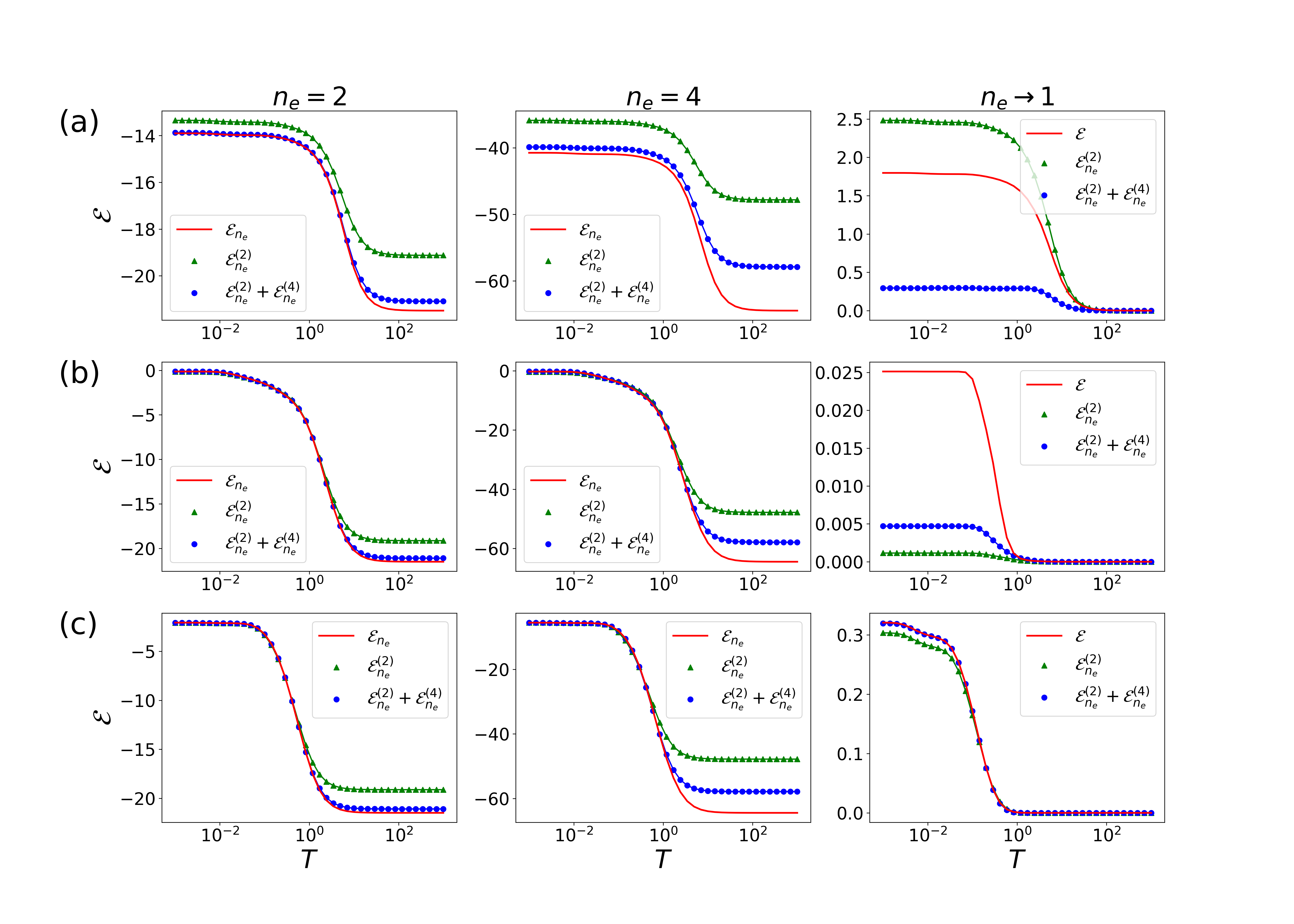
Figure 1: Numerical verification for the validity of charge correlator expansion (52) for $n_{e}=2,4$ and $n_{e}\rightarrow 1$ on thermal equilibrium states of 100-fermion system with conserved charge, i.e. $\rho=e^{-\beta H}/Z$, $\beta=1/T$ and $H=\sum_{i,j}t_{ij}c_{i}^{\dagger}c_{j}$. The amplitude of each $t_{ij}$ is randomly generated from a normal distribution, and the phase is generated from an even distribution in $[0,2\pi)$. The first two terms of the expansion (54) and (55) is calculated by (59) to (66), and the exact values of negativity are calculated by (70) and (71). The regions $A$ and $B$ are chosen to be the 21 to 30-th and 34 to 54-th fermions respectively. The quality of convergence depends on the pattern of the random Hamiltonian generated. (a) With random all-connected hopping $t_{ij}$, generated from the same distribution between all sites. (b) With random local hopping $t_{ij}$ for 1+1-d system. The amplitude of $t_{ij}$ exponentially decays with the distance $|i-j|$. (c) With random translational invariant local hopping $t_{ij}=t_{i-j,0}$ for 1+1-d system, within the distance of 3 atoms $|i-j|\leq 3$.

To check the validity of (52), we numerically calculate the expansion (54), (55), (56) and (57) in thermal equilibrium states of a 100-fermion system with randomly generated free Hamiltonian and conserved charge. It is well known that Rényi and von Neumann entropy of Gaussian states can be computed efficiently by relating to the two-point correlator matrices [27, 28, 29]. Both Rényi and logarithmic negativity of Gaussian states can also be related to correlator matrices, and so do the connected charge correlators. The correlator matrix of a bipartite system $A\cup B$ can be partitioned to block matrices as

$$C=\begin{pmatrix}C^{11}&C^{12}\\ C^{21}&C^{22}\end{pmatrix},$$ (58)

where the matrix elements are $C_{ij}=\braket{c_{i}^{\dagger}c_{j}}$. $C^{11}$ and $C^{22}$ are the reduced correlator matrices on the subsystems $A$ and $B$, and $C^{12}$ and $C^{21}$ contain correlation between two regions. Using Wick’s theorem, the connected charge correlators in the expansion can be reduced to the trace of the product of the block matrices as

$$\braket{Q_{A}^{2}}_{c}=\mathrm{Tr}C^{11}-\mathrm{Tr}(C^{11})^{2},$$ (59)

$$\braket{Q_{A}Q_{B}}_{c}=-\mathrm{Tr}(C^{12}C^{21}),$$ (60)

$$\braket{Q_{B}^{2}}_{c}=\mathrm{Tr}C^{22}-\mathrm{Tr}(C^{22})^{2},$$ (61)

$$\braket{Q_{A}^{4}}_{c}=\mathrm{Tr}C^{11}-7\mathrm{Tr}(C^{11})^{2}+12\mathrm{Tr}(C^{11})^{3}-6\mathrm{Tr}(C^{11})^{4},$$ (62)

$$\braket{Q_{A}^{3}Q_{B}}_{c}= -\mathrm{Tr}(C^{12}C^{21})+6\mathrm{Tr}(C^{11}C^{12}C^{21})$$ (63)

$$-6\mathrm{Tr}(C^{11}C^{11}C^{12}C^{21}),$$

$$\braket{Q_{A}^{2}Q_{B}^{2}}_{c}= -\mathrm{Tr}(C^{12}C^{21})+2\mathrm{Tr}(C^{11}C^{12}C^{21})$$ (64)

$$+2\mathrm{Tr}(C^{22}C^{21}C^{12})-4\mathrm{Tr}(C^{11}C^{12}C^{21}C^{12})$$

$$-2\mathrm{Tr}(C^{12}C^{21})^{2},$$

$$\braket{Q_{A}Q_{B}^{3}}_{c}= -\mathrm{Tr}(C^{12}C^{21})+6\mathrm{Tr}(C^{22}C^{21}C^{12})$$ (65)

$$-6\mathrm{Tr}(C^{22}C^{22}C^{21}C^{12}),$$

$$\braket{Q_{B}^{4}}_{c}=\mathrm{Tr}C^{22}-7\mathrm{Tr}(C^{22})^{2}+12\mathrm{Tr}(C^{22})^{3}-6\mathrm{Tr}(C^{22})^{4}.$$ (66)

To calculate the negativity of Gaussian states, we follow the method developed in [10] and [12]. Define the covariance matrices

$$\Gamma=\mathbb{I}-2C=\begin{pmatrix}\Gamma^{11}&\Gamma^{12}\\ \Gamma^{21}&\Gamma^{22}\end{pmatrix}$$ (67)

(where $\mathbb{I}$ is the identity matrix), the corresponding transformed matrices

$$\Gamma_{\pm}=\begin{pmatrix}-\Gamma^{11}&\pm i\Gamma^{12}\\ \pm i\Gamma^{21}&\Gamma^{22}\end{pmatrix},$$ (68)

and a new single particle correlation function

$$C_{\Xi}=\frac{1}{2}[\mathbb{I}-(\mathbb{I}+\Gamma_{+}\Gamma_{-})^{-1}(\Gamma_{+}+\Gamma_{-})].$$ (69)

Denoting $\zeta_{i}$ and $\xi_{i}$ as the eigenvalues of $C$ and $C_{\Xi}$ respectively, the logarithmic and Rényi negativity for free system with conserved charge is

$$\mathcal{E}=\sum_{j}\log[\xi_{j}^{1/2}+(1-\xi_{j})^{1/2}]+\frac{1}{2}\sum_{j}\log[\zeta_{j}^{2}+(1-\zeta_{j})^{2}]$$ (70)

and

$$\mathcal{E}_{n_{e}}= \sum_{j}\log[\xi_{j}^{n_{e}/2}+(1-\xi_{j})^{n_{e}/2}]$$ (71)

$$+\frac{n_{e}}{2}\sum_{j}\log[\zeta_{j}^{2}+(1-\zeta_{j})^{2}].$$

Using (59) to (66), we calculate the first two orders of the charge correlator expansion (54) and (55) and compare it with the exact $\mathcal{E}$ and $\mathcal{E}_{n_{e}}$ calculated by (70) and (71), see Fig. 1. From Fig. 1 (a)(b) we see that the convergence of Rényi negativity is generally fast even for all-connected Hamiltonian. When there are only local hopping terms that decays exponentially with the distance, which is the normal case for extensive systems, the convergence is extremely accurate at low temperature. For high temperature the convergence becomes slow, particularly for higher $n_{e}$. Note that these phenomena are all similar to the case of the expansion for Rényi and von Neumann entropy (36) and (37), where the convergence is better for systems with low temperature and local hopping terms.

However, the correspondence of the expansion at replica limit $n_{e}\rightarrow 1$ with logarithmic negativity requires more constraint. Fig.1 (b) shows the bad convergence even for local random Hamiltonian, from Fig.1 (c) we see that the convergence is valid for translational invariant systems. With translational symmetry, the convergence is also better in systems with local hopping terms.

Therefore, from numerical verification we conclude that the charge correlator expansion can be used to analyze the scaling behavior of Rényi negativity for local free Hamiltonian with conserved charge, while for logarithmic negativity it further requires translational invariance. In [10] it is numerically verified that the scaling behavior of negativity in Kitaev chain and SSH model (both with translational invariant Hamiltonian) is consistent with the CFT result from replica trick.

IV Applications

IV.1 (1+1)-d free fermion

(1+1)-d free-fermion systems with translational symmetry at zero temperature, with the Euler characteristic of the Fermi sea being $\chi_{F}$ (equals the number of segments of the Fermi sea), is also a CFT with central charge $c=\chi_{F}$ [13]. For (1+1)-d free-fermion systems, the $M=2$ term is related to $\chi_{F}$ and (4) becomes the universal second-order density correlator

$$\int\frac{dq^{\prime}}{2\pi}\braket{\rho_{q}\rho_{q^{\prime}}}_{c}=\chi_{F}|q|,$$ (72)

for small $q$. where $\rho_{q}$ is the charge density in momentum space

$$\rho_{q}=\int{dx}\rho(x)e^{-iqx}=\int\frac{dk}{2\pi}c_{k}^{\dagger}c_{k+q}.$$ (73)

After Fourier transformation we get density correlator $\braket{\rho(x_{1})\rho(x_{2})}_{c}$ in real space. Here we have to apply the invariance of correlator under translation in systems with translational symmetry by

$$\braket{\rho(x_{1})\rho(x_{2})}_{c} =\braket{\rho(x_{1}-x_{2})\rho(0)}_{c}$$ (74)

$$=\int\frac{dq}{2\pi}\frac{dq^{\prime}}{2\pi}\braket{\rho_{q}\rho_{q^{\prime}}}_{c}e^{iq(x_{1}-x_{2})}$$

$$=-\frac{\chi_{F}}{2\pi^{2}}\frac{1}{(x_{1}-x_{2})^{2}}.$$

(74) applies for large $x_{1}-x_{2}\gg\varepsilon$, where the short-distance cutoff $\varepsilon$ is about the inverse of the curvature of Fermi surface [13] (in 1d the length of the shortest segment or interval of Fermi sea).

To get charge correlator of regions we integrate (74) in real space. Now suppose we take the region $A:\ -l_{1}\leq x\leq 0$, $B:\ d\leq x\leq d+l_{2}$ and $C$ being the rest parts. For $\braket{Q_{A}^{2}}_{c}$ we encounter the case for short distance with small $x_{1}-x_{2}$. To solve this problem we consider a simplified model, where for $|x_{1}-x_{2}|>\varepsilon$

$$\braket{\rho(x_{1})\rho(x_{2})}_{c}=-\frac{\chi_{F}}{2\pi^{2}}\frac{1}{(x_{1}-x_{2})^{2}},$$ (75)

and for $|x_{1}-x_{2}|\leq\varepsilon$ it is a constant

$$\braket{\rho(x_{1})\rho(x_{2})}_{c}=-\frac{\chi_{F}}{2\pi^{2}}\frac{1}{\varepsilon^{2}}.$$ (76)

We consider the case that the regions $A,B$ are much larger than the short-distance cutoff, i.e. $l_{1},l_{2}\gg\varepsilon$. Therefore

$$\braket{Q_{A}^{2}}_{c} =\int_{-l_{1}}^{0}dx_{1}\int_{-l_{1}}^{0}dx_{2}\braket{\rho(x_{1})\rho(x_{2})}_{c}$$ (77)

$$=\frac{\chi_{F}}{2\pi^{2}}\left[2\log\frac{l_{1}}{\varepsilon}+O\left(\frac{l_{1}}{\varepsilon}\right)\right].$$

Similarly for $\braket{Q_{B}^{2}}_{c}$ we have

$$\braket{Q_{B}^{2}}_{c} =\frac{\chi_{F}}{2\pi^{2}}\left[2\log\frac{l_{2}}{\varepsilon}+O\left(\frac{l_{2}}{\varepsilon}\right)\right].$$ (78)

For $\braket{Q_{A}Q_{B}}_{c}$, at $d\geq\varepsilon$ the integration get

$$\braket{Q_{A}Q_{B}}_{c} =\int_{-l_{1}}^{0}dx_{1}\int_{d}^{d+l_{2}}dx_{2}\braket{\rho(x_{1})\rho(x_{2})}_{c}$$ (79)

$$=-\frac{\chi_{F}}{2\pi^{2}}\log\frac{(l_{1}+d)(l_{2}+d)}{d(l_{1}+l_{2}+d)}$$

and for $d<\varepsilon\ll l_{1},l_{2}$,

$$\braket{Q_{A}Q_{B}}_{c} =\int_{-l_{1}}^{0}dx_{1}\int_{d}^{d+l_{2}}dx_{2}\braket{\rho(x_{1})\rho(x_{2})}_{c}$$ (80)

$$=-\frac{\chi_{F}}{2\pi^{2}}\left[\log\frac{(l_{1}+d)(l_{2}+d)}{\varepsilon(l_{1}+l_{2}+d)}+O\left(\frac{d}{\varepsilon}\right)\right]$$

$$=-\frac{\chi_{F}}{2\pi^{2}}\log\frac{l_{1}l_{2}}{\varepsilon(l_{1}+l_{2})}.$$

In the last step we ignore the small $O(d/\varepsilon)$ terms. With the above results for charge correlators, for $d\gg\varepsilon$ (54) becomes

$$\mathcal{E}_{n_{e}}^{(2)}= \chi_{F}\left[-\frac{n_{e}^{2}-1}{6n_{e}}\left(\log\frac{l_{1}l_{2}}{\varepsilon^{2}}+O\left(\frac{l}{\varepsilon}\right)\right)\right.$$ (81)

$$+\left.\frac{n_{e}^{2}+2}{12n_{e}}\log\frac{(l_{1}+d)(l_{2}+d)}{d(l_{1}+l_{2}+d)}\right].$$

And for $d\rightarrow 0$ it becomes

$$\mathcal{E}_{n_{e}}^{(2)}= \chi_{F}\left[-\frac{n_{e}^{2}-1}{6n_{e}}\left(\log\frac{l_{1}l_{2}}{\varepsilon^{2}}+O\left(\frac{l}{\varepsilon}\right)\right)\right.$$ (82)

$$+\left.\frac{n_{e}^{2}+2}{12n_{e}}\log\frac{l_{1}l_{2}}{\varepsilon(l_{1}+l_{2})}\right].$$

First we consider the case $d\rightarrow 0$, i.e. regions $A$ and $B$ are adjacent, (82) can also be written as

$$\mathcal{E}_{n_{e}}^{(2)}=\chi_{F} \left[-\frac{n_{e}^{2}-4}{12n_{e}}\log\frac{l_{1}l_{2}}{\varepsilon^{2}}-\frac{n_{e}^{2}+2}{12n_{e}}\log\frac{l_{1}+l_{2}}{\varepsilon^{2}}\right.$$ (83)

$$\left.-\frac{n_{e}^{2}-1}{6n_{e}}O\left(\frac{l}{\varepsilon}\right)\right],$$

which is identical to (85) in [10] at even $n_{e}$ except for the short distance cutoff (note that the term for short distance cutoff $O\left(l/{\varepsilon}\right)$ is generally large and cannot be neglected). Taking the limit $n_{e}\rightarrow 1$ we get

$$\mathcal{E}_{n_{e}\rightarrow 1}^{(2)}=\frac{\chi_{F}}{4}\log\frac{l_{1}l_{2}}{\varepsilon(l_{1}+l_{2})}.$$ (84)

Then the first term related to divergent short-distance cutoff is eliminated, which is consistent with what we expect for negativity. Numerical checks in Sec. III have confirmed that for system with translational symmetry, the expansion of $\mathcal{E}_{n_{e}\rightarrow 1}$ converges to $\mathcal{E}$, so (84) captures the scaling property of $\mathcal{E}$.

We can also consider the cases that region $A$ and $B$ are far apart, i.e. $d\gg l_{1},l_{2}$. Then (81) can be expanded to the second order of $l_{i}/d$ as

$$\mathcal{E}_{n_{e}}^{(2)}=\chi_{F} \left[-\frac{n_{e}^{2}-1}{6n_{e}}\left(\log\frac{l_{1}l_{2}}{\varepsilon^{2}}+O\left(\frac{l}{\varepsilon}\right)\right)\right.$$ (85)

$$+\left.\frac{n_{e}^{2}+2}{12n_{e}}\frac{l_{1}l_{2}}{d^{2}}\right].$$

Taking the limit $n_{e}\rightarrow 1$ the first term vanishes and we also get rid of the short-distance cutoff

$$\mathcal{E}_{n_{e}\rightarrow 1}^{(2)}=\frac{\chi_{F}}{4}\frac{l_{1}l_{2}}{d^{2}}.$$ (86)

Therefore it is proportional to the length of the two regions and decays with the distance by a power law.

IV.2 free fermion in higher dimension

Similar to the 1+1-dimensional case, we consider free-fermion system with conserved charge in $(D+1)$-dimension. Here we consider region $A$ and $B$ to be two balls with radius $R_{1},R_{2}$ and the distance between their centers $d\gg R_{1},R_{2}$. In higher dimensions the $M$-th order connected charge correlator satisfies

$$\int\frac{d\bm{q}_{M}}{2\pi}\braket{\rho_{\bm{q}_{1}}\cdots\rho_{\bm{q}_{M}}}_{c}\sim k_{F}^{D+1-M}q^{M-1}$$ (87)

for small $\bm{q}$ [13], where $q$ is the typical length of $\bm{q}_{i}$, $i=1,\cdots M-1$. In (54) the second order correlator is

$$\int\frac{d\bm{q}^{\prime}}{2\pi}\braket{\rho_{\bm{q}}\rho_{\bm{q}^{\prime}}}_{c}\sim k_{F}^{D-1}|\bm{q}|.$$ (88)

by Fourier transformation it gives the real space correlator

$$\braket{\rho(\bm{r}_{1})\rho(\bm{r}_{2})}_{c}\sim\frac{k_{F}^{D-1}}{|\bm{r}_{1}-\bm{r}_{2}|^{D+1}},$$ (89)

for $|\bm{r}_{1}-\bm{r}_{2}|\gg\varepsilon$. Taking the similar model for short distance cutoff as the 1+1-d case, the integral in real space gives

$$\braket{Q_{A}^{2}}_{c} \sim(k_{F}R_{1})^{D-1}\left(1+O\left(\frac{R_{1}}{\varepsilon}\right)\right),$$ (90)

$$\braket{Q_{B}^{2}}_{c} \sim(k_{F}R_{2})^{D-1}\left(1+O\left(\frac{R_{2}}{\varepsilon}\right)\right),$$ (91)

and

$$\braket{Q_{A}Q_{B}}_{c} \sim k_{F}^{D-1}\frac{R_{1}^{D}R_{2}^{D}}{d^{D+1}}.$$ (92)

Therefore (54) becomes

$$\mathcal{E}_{n_{e}}^{(2)}\sim k_{F}^{D-1}\left[c_{1}\frac{n_{e}^{2}-1}{6n_{e}}\left(R_{1}^{D-1}+R_{2}^{D-1}+O\left(\frac{R}{\varepsilon}\right)\right)\right.$$ (93)

$$\left.+c_{2}\frac{n_{e}^{2}+2}{6n_{e}}\frac{R_{1}^{D}R_{2}^{D}}{d^{D+1}}\right],$$

where $c_{1},c_{2}$ are some finite coefficient. We see that when regions $A$ and $B$ are far apart, the terms from $\braket{Q_{A}^{2}}_{c}$ and $\braket{Q_{B}^{2}}_{c}$ contain a constant term with short-distance cutoff that do not depend on the distance between $A$ and $B$, and is much larger than the terms from $\braket{Q_{A}Q_{B}}_{c}$. This incidates that Rényi negativity is not a good entanglement measure. However, at replica limit $n_{e}\rightarrow 1$, the first term with short distance cutoff is also eliminated, and we get

$$\mathcal{E}_{n_{e}\rightarrow 1}^{(2)}\sim k_{F}^{D-1}\frac{R_{1}^{D}R_{2}^{D}}{d^{D+1}}.$$ (94)

This is consistent with our expectation for logarithmic negativity as an entanglement measure. The negativity is proportional to the area of two regions and decays also by a power law with the distance between them.

V Conclusion and discussion

In this paper, we derive the connected charge correlator expansion for Rényi and logarithmic negativity in free-fermion systems with conserved $U(1)$ charge. We numerically check the validity of the expansion, and find that the convergence at replica limit requires translational symmetry. Using this expansion, we analyze the scaling behavior of negativity in extensive free-fermion systems. From the expansion, it is direct to note that there are terms that diverge for short distance cutoff in the expansion for Rényi negativity, but they vanish at the limit $n_{e}\rightarrow 1$. This is consistent with our expectation for logarithmic negativity rather than Rényi negativity as an entanglement measure.

Our research in charge correlator expansion is generally limited to free-fermion systems. One can also consider canonical bosonic systems where the charge operator is similarly defined, but will encounter difficulty in the range of $p$ (34). For bosonic systems, the range of $p$ is given by $p=0,1,\cdots,n-1\ (\mathrm{mod}\ n)$. There seems to be no natural choice of the range to make the summation $\sum_{p}p^{M}$ smallest for even $M$ and 0 for odd $M$, as required for the convergence in fermionic systems. As a consequence, we cannot obtain the correct coefficient in the expansion after the terms with higher $M$ are truncated. Spin systems may also be considered, but the charge operator is hard to define, and free-spin systems (without spin-spin interaction) may not be intriguing for research.

The charge expansion may also be applied to other computable entanglement measures besides PT negativity, e.g. the computable cross norm or realignment (CCNR) negativity [30, 31, 32]. Recently, it has been shown that Rényi and logarithmic CCNR negativity of two intervals that are not adjacent has a universal expression [33] in (1+1)-d CFT. The twist operators for CCNR negativity cannot be simultaneously diagonalized, but they can be simultaneously block diagonalized in the form of $2\times 2$ matrices. Therefore CCNR negativity can be in free systems can be related to the expectation value of $2\times 2$ operators instead of $U(1)$ charge operators. We suppose that the charge expansion for these computable entanglement measures can provide a deeper understanding of the entanglement properties of quantum systems.

Formula (4) shows that the universal $(D+1)$-th order charge correlator in $D$-dimensional free-fermion systems is proportional to the Euler characteristic of the Fermi sea. The leading term in the expansion for Rényi and logarithmic negativity (54) and (56) contains second-order charge correlators, and therefore in (1+1)-d system, it extracts the Euler characteristic, as shown in Sec. IV.1. However, for higher dimensions, the divergent terms always exist in the leading term. It is an interesting question whether there are ways to subtract the divergent terms and extract topological terms in the expansion for negativity, like the case for topological entanglement entropy [13].

Appendix A Cumulant expansion for Rényi and von Neumann entropy

From (33)

$$\log\braket{T_{n}} =\sum_{M=1}^{\infty}\left(\sum_{p}p^{M}\right)\frac{1}{M!}\left(\frac{2\pi i}{n}\right)^{M}\braket{Q_{A}^{M}}_{c},$$ (95)

the summation of $p$ is

$$C_{n,M}=\sum_{p=-\frac{n-1}{2}}^{\frac{n-1}{2}}p^{M}$$ (96)

It can be written in the form of generalized harmonic number [34]

$$H_{n}^{(s)}(z)=\sum_{j=1}^{n}\frac{1}{(j+z)^{s}}\ \ \ \ (n\in\mathbb{Z}^{+},s\in\mathbb{C},z\in\mathbb{C}\backslash\mathbb{Z}^{-}).$$ (97)

First consider the case of even $n$, the result is

$$\sum_{p=-\frac{n-1}{2}}^{\frac{n-1}{2}}p^{M} =\left[1+(-1)^{M}\right]\times\left[\left(\frac{1}{2}\right)^{M}+\left(\frac{3}{2}\right)^{M}+\cdots+\left(\frac{n-1}{2}\right)^{M}\right]$$ (98)

$$=\begin{cases}2H_{n/2}^{(-M)}\left(-\frac{1}{2}\right)\ &\mathrm{even}\ M\\ 0\ &\mathrm{odd}\ M.\end{cases}$$

For the range of arguments we consider here, the generalized harmonic number is related to the generalized Riemann zeta function (this is generally not correct).

$$\zeta(n,a)=\sum_{k=0}^{\infty}\frac{1}{(k+a)^{n}}$$ (99)

by

$$H_{n}^{(s)}(z)=\zeta(s,z+1)-\zeta(s,z+n+1)$$ (100)

and $\zeta(n)=\zeta(n,1)$. Thus

$$\log\braket{T_{n}} =\sum_{\begin{subarray}{c}M=2\\ \mathrm{even}\ M\end{subarray}}^{\infty}2H_{n/2}^{(-M)}\left(-\frac{1}{2}\right)\frac{1}{M!}\left(\frac{2\pi i}{n}\right)^{M}\braket{Q_{A}^{M}}_{c}$$ (101)

$$=\sum_{\begin{subarray}{c}M=2\\ \mathrm{even}\ M\end{subarray}}^{\infty}2\left[\zeta\left(-M,\frac{1}{2}\right)-\zeta\left(-M,\frac{n+1}{2}\right)\right]\frac{1}{M!}\left(\frac{2\pi i}{n}\right)^{M}\braket{Q_{A}^{M}}_{c}.$$

For even $M\geq 0$, $\zeta\left(-M,1/2\right)=0$, we get

$$\log\braket{T_{n}} =-\sum_{\begin{subarray}{c}M=2\\ \mathrm{even}\ M\end{subarray}}^{\infty}2\zeta\left(-M,\frac{n+1}{2}\right)\frac{1}{M!}\left(\frac{2\pi i}{n}\right)^{M}\braket{Q_{A}^{M}}_{c}.$$ (102)

For odd $n$, it is easy to check that we get

$$\log\braket{T_{n}} =\sum_{\begin{subarray}{c}M=2\\ \mathrm{even}\ M\end{subarray}}^{\infty}2H_{(n-1)/2}^{(-M)}\left(0\right)\frac{1}{M!}\left(\frac{2\pi i}{n}\right)^{M}\braket{Q_{A}^{M}}_{c}$$ (103)

$$=\sum_{\begin{subarray}{c}M=2\\ \mathrm{even}\ M\end{subarray}}^{\infty}2\left[\zeta\left(-M,1\right)-\zeta\left(-M,\frac{n+1}{2}\right)\right]\frac{1}{M!}\left(\frac{2\pi i}{n}\right)^{M}\braket{Q_{A}^{M}}_{c}.$$

For even $M\geq 0$, $\zeta\left(-M,1\right)=0$, thus we get the same result

$$\log\braket{T_{n}} =-\sum_{\begin{subarray}{c}M=2\\ \mathrm{even}\ M\end{subarray}}^{\infty}2\zeta\left(-M,\frac{n+1}{2}\right)\frac{1}{M!}\left(\frac{2\pi i}{n}\right)^{M}\braket{Q_{A}^{M}}_{c}.$$ (104)

This gives the cumulant expansion for Rényi entropy (36).

Since the right hand side of (104) is real for all positive integer $n$, we now extend it from $n\in\mathbb{Z}^{+}$ to $n\in\mathbb{R}^{+}$ and calculate the von Neumann entropy by taking the $n\rightarrow 1$ limit. The analytic continuation can differ with periodic functions and affect the result, but we assume it is correct here. By using

$$\frac{d}{dn}\zeta(k,n)=-k\zeta(k+1,n),$$ (105)

we get

$$S_{A} =\lim_{n\rightarrow 1}\frac{\log\braket{T_{n}}}{1-n}=\sum_{\begin{subarray}{c}M=2\\ \mathrm{even}\ M\end{subarray}}^{\infty}2\left.\frac{d}{dn}\zeta\left(-M,\frac{n+1}{2}\right)\right|_{n=1}\frac{1}{M!}({2\pi i})^{M}\braket{Q_{A}^{M}}_{c}$$ (106)

$$=\sum_{\begin{subarray}{c}M=2\\ \mathrm{even}\ M\end{subarray}}^{\infty}M\left.\zeta\left(1-M,\frac{n+1}{2}\right)\right|_{n=1}\frac{1}{M!}({2\pi i})^{M}\braket{Q_{A}^{M}}_{c}.$$

And by using the relation

$$\zeta(1-M)=2(2\pi)^{-M}\cos(\pi M/2)(M-1)!\zeta(M),$$ (107)

we get

$$S_{A} =\sum_{\begin{subarray}{c}M=2\\ \mathrm{even}\ M\end{subarray}}^{\infty}M\zeta\left(1-M,1\right)\frac{1}{M!}({2\pi i})^{M}\braket{Q_{A}^{M}}_{c}$$ (108)

$$=\sum_{\begin{subarray}{c}M=2\\ \mathrm{even}\ M\end{subarray}}^{\infty}2\zeta(M)\braket{Q_{A}^{M}}_{c}.$$

This is the cumulant expansion for von Neumann entropy (37).