Statistical Test for Anomaly Detections by Variational Auto-Encoders

Abstract

In this study, we consider the reliability assessment of anomaly detection (AD) using Variational Autoencoder (VAE). Over the last decade, VAE-based AD has been actively studied in various perspective, from method development to applied research. However, when the results of ADs are used in high-stakes decision-making, such as in medical diagnosis, it is necessary to ensure the reliability of the detected anomalies. In this study, we propose the VAE-AD Test as a method for quantifying the statistical reliability of VAE-based AD within the framework of statistical testing. Using the VAE-AD Test, the reliability of the anomaly regions detected by a VAE can be quantified in the form of $p$-values. This means that if an anomaly is declared when the $p$-value is below a certain threshold, it is possible to control the probability of false detection to a desired level. Since the VAE-AD Test is constructed based on a new statistical inference framework called selective inference, its validity is theoretically guaranteed in finite samples. To demonstrate the validity and effectiveness of the proposed VAE-AD Test, numerical experiments on artificial data and applications to brain image analysis are conducted.

1 Introduction

Anomaly detection (AD) is the process of identifying unusual deviations in data that do not conform to expected behavior. AD is crucial across various domains because it provides early warnings of potential issues, thereby enabling timely interventions to prevent critical events. Traditional AD techniques, while effective in straightforward scenarios, frequently fall short when dealing with complex data, thus motivating the use of deep learning-based AD approaches to better handle such complexities. In this study, among various deep learning-based AD approaches, we focus on AD using the Variational Auto-Encoder (VAE), and its application to medical images.

A VAE serves as an effective tool for AD task. In the training phase, the VAE learns the distribution of normal images by training exclusively on images that do not contain abnormal regions. It encodes the input image into a latent space and then reconstructs it back to its original form. The parameters of a VAE are optimized to minimize the reconstruction error, thereby learning a compressed representation of the normal data. In the test phase, when a test image is fed into the trained VAE, the model attempts to reconstruct the image based on its learned representation. The reconstruction error is then calculated, typically as the difference between the input image and its reconstructed version. Since the VAE is trained on normal data, it would successfully reconstruct the normal regions of the image, while it would fail to properly reconstruct the abnormal regions that were not included in the normal data. Therefore, regions with large reconstruction errors are detected as abnormal regions. Figure 1 shows an example of VAE-based AD for brain tumor images.

When VAE-based AD is employed for high-stakes decision-making tasks, such as medical diagnosis, there is a significant risk that model inaccuracies might lead to critical errors, potentially resulting in false detections. To address this issue, in this study, we develop a statistical test for VAE-based AD, which we call VAE-AD Test. The proposed VAE-AD test enables us to obtain a quantifiable and interpretable measure for the detected anomaly region in the form of $p$-value. The obtained $p$-value represents the probability that the detected anomaly regions are obtained by chance due to the randomness contained in the data. For example, if we adopt a rule that classifies detected anomaly regions with a $p$-value less than 0.05 as anomalies, we can keep the false detection probability below 5% rigorously.

It is important to note that the statistical test for detected abnormal regions is performed on data-driven hypothesis, as the abnormal region is selected based on the test image itself. In other words, since both of the selection of the hypothesis (selection of abnormal regions) and the evaluation of the hypothesis (evaluation of abnormal regions) are performed on the same data, applying traditional statistical test to the selected hypothesis (abnormal regions) leads to selection bias. Therefore, in this study, we introduce the framework of Conditional Selective Inference (CSI), which has been recognized as a new statistical testing framework for data-driven hypotheses. CSI has primarily been studied in the context of feature selection for linear models, but in recent years, it has been extended to various problems in various models (see the related works section for more details).

The main contributions in this study are the following three points. Our first contribution is the formulation of an approach that provides a quantifiable and interpretable measure for the reliability of anomalies detected by VAE in the form of a $p$-value based on a statistical test. With this approach, we can properly control the probability of false detection probability to the desired significance level in finite samples. The second contribution is the development of an SI method for VAEs. SI is formulated as a conditional test based on the conditions under which hypotheses are selected (see §3 for details), requiring computations concerning the hypothesis selection event by a VAE. Our main technical contribution is to establish a method to compute the hypothesis selection event for a wide class of VAEs. Finally, the third contribution is to demonstrate the effectiveness of the proposed VAE-AD Test by conducting numerical experiments with synthetic data and brain tumor images. The code is available at https://github.com/DaikiMiwa/VAE-AD-Test.

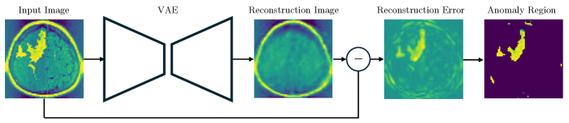
(a) Image without tumor region. $p_{\rm naive}=0.000$ (false detection) and $p_{\rm selective}=0.668$  (true negative).

(b) Image with tumor region. $p_{\rm naive}=0.000$ (true detection) and $p_{\rm selective}=0.000$ (true detection).

Figure 1: An illustration of the proposed VAE-AD Test in brain image analysis. When an anomaly region is detected based on the difference between the original image and the reconstructed image by a VAE, the VAE-AD Test provides a $p$-value to quantify its statistical reliability. The upper plot shows the results of applying the VAE-AD Test and the conventional method, which does not consider the fact that the anomaly region is detected by VAE, to a case without anomaly regions. The lower plot shows the results for a case with anomaly regions. With the proposed method ($p_{\rm selective}$), correct judgments are made in both cases; the former has a large $p$-value and the latter has a small $p$-value. In contrast, with the conventional method ($p_{\rm naive}$), both $p$-values are small, indicating false detection in the former case.

1.1 Related Work

Over the last decade, there has been a significant pursuit in applying deep learning techniques to AD problems (Chalapathy and Chawla, 2019; Pang et al., 2021; Tao et al., 2022). A large number of studies have been conducted for unsupervised AD using VAEs (Baur et al., 2021; Chen and Konukoglu, 2018; Chow et al., 2020; Jana et al., 2022). VAE-based AD for images is broadly divided into two tasks. The first task is to determine whether the entire input image is normal or abnormal. The second task is to detect abnormal regions within the input image, which is sometimes referred to as anomaly localization (Zimmerer et al., 2019; Lu and Xu, 2018; Baur et al., 2019). In this study, we focus on the second task. There are mainly two research directions for improving VAEs for AD. The first direction is on improving the indicators of the degree of anomaly (Zimmerer et al., 2019; Dehaene et al., 2020). The second direction is on modifying the VAE itself to make it suitable for AD (Baur et al., 2019; Chen and Konukoglu, 2018; Wang et al., 2020). However, to our knowledge, there has been no existing studies for quantifying the statistical reliability of detected abnormal regions with theoretical validity.

In traditional statistical tests, the hypothesis needs to be predetermined and must remain independent of the data. However, in data-driven approaches, it is necessary to select hypotheses based on the data and then assess the reliability of the hypotheses using the same data. This issue, known as double dipping, arises because the same data is used for both the selection and evaluation of hypotheses, leading to selection bias (Breiman, 1992). Because anomalies are detected based on data (a test image) in AD, when evaluating the reliability of the detected anomalies using the same data, the issue of selection bias arises. CSI has recently gained attention as a framework for statistical hypothesis testing of data-driven hypotheses Lee et al. (2016); Taylor and Tibshirani (2015). The key idea of CSI is to address the selection bias issue by considering a conditional test. CSI was initially developed for the statistical inference of feature selection in linear models (Fithian et al., 2015; Tibshirani et al., 2016; Loftus and Taylor, 2014; Suzumura et al., 2017; Le Duy and Takeuchi, 2021; Sugiyama et al., 2021), and then extended to various problems (Lee et al., 2015; Choi et al., 2017; Chen and Bien, 2020; Tanizaki et al., 2020; Duy et al., 2020; Gao et al., 2022). CSI was first introduced to deep learning context in Duy et al. (2022) and Miwa et al. (2023), with the former focusing on evaluating the reliability of segmentation and the latter aiming to assess the reliability of the saliency map. In this paper, we develop CSI for VAEs based on these studies and establish a framework for quantitatively evaluating the reliability of VAE-based AD.

2 Anomaly Detection (AD) by VAE

In this section, we present how VAEs are used for AD.

2.1 Variational Autoencoder (VAE)

VAEs are generative models originally proposed by Kingma and Welling (2013). A VAE consists of an encoder network and a decoder network. Given an input image (denoted by $\bm{x}\in\mathbb{R}^{n}$), it is encoded as a latent vector (denoted by $\bm{z}\in\mathbb{R}^{m}$), and the latent vector is decoded back to the input image, where $n$ is the number of pixels of an image and $m$ is the dimension of a latent vector. In the generative process, it is assumed that a latent vector $\bm{z}$ is sampled from a prior distribution $p_{\bm{\theta^{*}}}(\bm{z})$ and then, image $\bm{x}$ is sampled from a conditional distribution $p_{\bm{\theta}^{*}}(\bm{x}|\bm{z})$. The prior distribution $p_{\bm{\theta}^{*}}(\bm{z})$ and the conditional distribution $p_{\bm{\theta}^{*}}(\bm{x}|\bm{z})$ belongs to family of distributions parametrized by $\bm{\theta}$ and $\bm{\theta^{*}}$ denotes the true value of the parameter.

Since the posterior distribution $p_{\bm{\theta}}(\bm{z}|\bm{x})$ is assumed to be intractable, the encoder network approximates it by the parametric distribution $q_{\bm{\phi}}(\bm{z}|\bm{x})$, where $\bm{\phi}$ represents the set of parameters. The decoder network estimate the conditional distribution by $p_{\bm{\theta}}(\bm{x}|\bm{z})$. The encoder and the decoder networks of a VAE are trained by maximizing so-called evidence lower bound (ELBO):

$$L_{\bm{\theta},\bm{\phi}}=\mathbb{E}_{q_{\bm{\theta}}(\bm{z}|\bm{x})}\left[\log p_{\bm{\phi}}(\bm{x}|\bm{z})\right]-\mathrm{KL}\left[q_{\bm{\theta}}(\bm{z}|\bm{x})||p(\bm{z})\right],$$

where $\mathrm{KL}\left[\cdot||\cdot\right]$ is the Kullback-Leibler divergence between two distributions.

In this study, we model the approximated posterior distribution $q_{\bm{\phi}}(\bm{z}|\bm{x})$ as a normal distribution, represented by $N(\bm{\mu}_{\bm{\phi}}(\bm{x}),I_{n}\bm{\sigma}_{\bm{\phi}}^{2}(\bm{x}))$, where $\bm{\mu}_{\bm{\phi}}(\bm{x})$ and $\bm{\sigma}^{2}_{\bm{\phi}}(\bm{x})$ are the outputs of the encoder network, and the condiional distribution $p_{\bm{\theta}}(\bm{x}|\bm{z})$ as a normal distribution, represented by $N(\bm{\mu}_{\bm{\theta}}(\bm{z}),I_{n})$, where $\bm{\mu}_{\bm{\theta}}(\bm{z})$ is the outputs of the decoder network. The prior distribution $p_{\bm{\theta}^{*}}(\bm{z})$ is modeld as a standard normal distribution $N(0,I_{m})$. The structure of the VAE used in this study is shown in Appendix A.

2.2 Anomaly Detection Using VAEs

VAEs can be effectively used for AD task. As outlined in §1, AD tasks can be categorized into two types: anomaly detection (in a narrow sense) and anomaly localization. This paper concentrates on anomaly localization whose goal is to identify the abnormal region within a given test image.

In the training phase, we assume that only normal images (e.g., brain images without tumors) are available. A VAE is trained on normal images to learn a compact representation of the normal image distribution in the latent space.

In the test phase, a test image $\bm{x}$ is fed into the trained VAE, and a reconstructed image is obtained by using the encoder and the decoder as $\hat{\bm{x}}=\bm{\mu}_{\bm{\theta}}\left(\bm{\mu}_{\bm{\phi}}(\bm{x})\right)$. Since the VAE is trained only on normal images, normal region in the test image would be reconstructed well, whereas the reconstruction error of abnormal regions would be high. Therefore, it is reasonable to define the degree of anomaly of each pixel as

$$E_{i}(\bm{x})=|x_{i}-\hat{x}_{i}|,i\in[n],$$ (1)

where $x_{i}$ and $\hat{x}_{i}$ is the $i^{\rm th}$ pixel value of $\bm{x}$ and $\hat{\bm{x}}$, respectively. Using a user-specified threshold $\lambda>0$, the anomaly region of a test image $\bm{x}$ is defined as

$$A_{\bm{x}}=\{i\in|n|\mid E_{i}(\bm{x})\geq\lambda\}.$$ (2)

As for the definition of the anomaly region, there are possibilities other than those given by Eqs. (1) and (2). In this paper, we proceed with these choices, but the proposed VAE-AD Test is generally applicable to other choices.

3 Statistical Test for Abnormal Regions

In this section, we formulate a statistical test for abnormal region $A$ in Eq. (2).

Statistical model of an image.

To formulate the reliability assessment of the abnormal region as a statistical testing problem, it is necessary to introduce a statistical model of an image. In this study, an image is considered as a sum of true signal component $\bm{s}\in\mathbb{R}^{n}$ and noise component $\bm{\epsilon}\in\mathbb{R}^{n}$. Regarding the true signal component, each pixel can have an arbitrary true signal value without any particular assumption or constraint. On the other hand, regarding the noise component, it is assumed to follow a normal distribution, and their covariance matrix is estimated using normal data different from that used for the training of the VAE. Namely, an image with $n$ pixels can be represented as an $n$-dimensional random vector

$$\bm{X}=(X_{1},\ldots,X_{n})=\bm{s}+\bm{\epsilon},\;\bm{\epsilon}\sim N(\bm{0},\Sigma),$$ (3)

where $\bm{\bm{s}}\in\mathbb{R}^{n}$ is the true signal vectors, and $\bm{\epsilon}\in\mathbb{R}^{n}$ is the noise vector with covariance matrix $\Sigma$. In the following, the capital $\bm{X}$ denotes an image as a random vector, while the lowercase $\bm{x}$ represents an observed image. To formulate the statistical test, we consider the AD using VAEs defined in Eq. (2) as a function ${\mathcal{A}}$ that maps a random input image $\bm{X}$ to the abnormal region $A_{\bm{X}}$, i.e.,

$${\mathcal{A}}:\mathbb{R}^{n}\ni\bm{X}\mapsto A_{\bm{X}}\in 2^{[n]},$$ (4)

where $2^{[n]}$ is the power set of $[n]:=\{1,2,\ldots,n\}$.

Formulation of statistical test.

Our goal is to make a judgment whether the abnormal region $A_{\bm{X}}$ merely appears abnormal due to the influence of random noise, or if there is a true anomaly in the true signal in the abnormal region. In order to quantify the reliability of the detected abnormal region, the statistical test is performed for the difference between the true signal in the abnormal region $\{s_{i}\}_{i\in A_{\bm{X}}}$ and the true signal in the normal region $\{s_{i}\}_{i\in A^{c}_{\bm{X}}}$ where $A^{c}_{\bm{X}}$ is the complement of the abnormal region. In this study, as an example, we consider the hypothesis for the difference in true mean signals between $A_{\bm{X}}$ and $A^{c}_{\bm{X}}$ by considering the following null and alternative hypotheses:

$$\begin{split}{\rm H}_{0}:\frac{1}{|A_{\bm{X}}|}\sum_{i\in A_{\bm{X}}}s_{i}&=\frac{1}{|A_{\bm{X}}^{c}|}\sum_{i\in A^{c}_{\bm{X}}}s_{i},\\ &{\rm v.s.}\\ {\rm H}_{1}:\frac{1}{|A_{\bm{X}}|}\sum_{i\in A_{\bm{X}}}s_{i}&\neq\frac{1}{|A_{\bm{X}}^{c}|}\sum_{i\in A_{\bm{X}}^{c}}s_{i}.\end{split}$$ (5)

For clarity, we mainly consider a test for the mean difference as a specific example — however, the proposed VAE-AD Test is applicable to a more general class of statistical tests. Specifically, let $\bm{\eta}\in\mathbb{R}^{n}$ be an arbitrary $n$-dimensional vector depending on the abnormal region $A_{\bm{X}}$. Then, the proposed method can cover a statistical test represented as

$$\begin{split}{\rm H}_{0}:\bm{\eta}^{\top}\bm{s}=c~{}~{}~{}{\rm v.s.}~{}~{}~{}{\rm H}_{1}:\bm{\eta}^{\top}\bm{s}\neq c,\end{split}$$ (6)

where $c$ is an arbitrary constant. The formulation in Eq. (6) covers a wide range of practically useful statistical tests. In fact, Eq. (5) is a special case of Eq. (6). It can cover differences not only in means but also in other measures such as maximum difference, and differences after applying some image filters (e.g., Gaussian filter).

Test statistic.

To evaluate the hypothesis defined in Eq. (5), we define the test statistic $T(\bm{X})$ as follows:

$$T(\bm{X})=\frac{1}{|A_{\bm{X}}|}\sum_{i\in A_{\bm{X}}}X_{i}-\frac{1}{|A_{\bm{X}}^{c}|}\sum_{i\in A_{\bm{X}}^{c}}X_{i}=\bm{\eta}^{\top}\bm{X},$$ (7)

where $\bm{\eta}=\frac{1}{|A_{\bm{X}}|}\bm{1}_{A_{\bm{X}}}-\frac{1}{|A_{\bm{X}}^{c}|}\bm{1}_{A_{\bm{X}}^{c}}$ and $\bm{1}_{A}\in\mathbb{R}^{n}$ is a vector whose $i$-th element is $1$ if $i\in A_{\bm{X}}$ and 0 otherwise.

Naive $p$-values.

When the test statistic in Eq. (7) is used for the statistical test in Eq. (5), the $p$-value can be easily calculated if $\bm{\eta}$ does not depend on the image $\bm{X}$, i.e., if the abnormal region $A_{\bm{X}}$ is detected without looking at the $\bm{X}$. In this unrealistic situation, the $p$-value, which we call naive $p$-value can be computed as

$$p_{\rm naive}=\mathbb{P}_{\rm H_{0}}(|T(\bm{X})|\geq|T(\bm{x})|),$$

where $\bm{X}$ is a random vector and $\bm{x}$ is the observed image. Under the unrealistic assumption, the $p_{\rm naive}$ can be easily computed because the null distribution of $T(\bm{X})=\bm{\eta}^{\top}\bm{X}$ is normally distributed with $N(0,\bm{\eta}^{\top}\Sigma\bm{\eta})$. Unfortunately, however, in the actual situation where $\bm{\eta}$ depends on $\bm{X}$, a statistical test using $p_{\rm naive}$ is invalid in the sense that

$${P}_{{\rm H}_{0}}(p_{\rm naive}\leq\alpha)>\alpha,\;\exists\alpha\in[0,1].$$

Namely, the probability of Type I error (an error that a normal region is mistakenly detected as anomaly) cannot be controlled at the desired significance level $\alpha$.

4 CSI for VAE-based AD

To obtain a valid $p$-value, we employ CSI framework.

4.1 Condtional Selective Inference (CSI)

In CSI, $p$-values are computed based on the null distribution conditional on a event that a certain hypothesis is selected. The goal of CSI is to compute a $p$-value that satisfies

$$P_{{\rm H}_{0}}(p\leq\alpha\mid A_{\bm{X}}=A)\leq\alpha,$$ (8)

where the condition part $A_{\bm{X}}=A$ in Eq. (8) indicates that we only consider images $\bm{X}$ for which a certain hypothesis (abnormal region) $A$ is detected. If the conditional type I error can be controlled as in Eq. (8) for all possible hypotheses $A\in 2^{[n]}$, then, by the law of total probability, the marginal type I error can also be controlled for all $\alpha\in(0,1)$ because

$$P_{{\rm H}_{0}}(p\leq\alpha)=\sum_{A\in 2^{[n]}}P_{{\rm H}_{0}}(A)(p\leq\alpha\mid A_{\bm{X}}=A)\leq\alpha.$$

Therefore, in order to perform valid statistical test, we can employ $p$-values conditional on the hypothesis selection event. To compute a $p$-value that satisfies Eq. (8), we need to derive the sampling distribution of the test-statistic

$$T(\bm{X})|\{A_{\bm{X}}=A_{\bm{x}}\}.$$ (9)

As stated in §1, CSI has gained attention as a method of statistical inference for feature selection in linear models (Lee et al., 2016). Most of the existing SI studies exploit the fact that a hypothesis selection event (e.g., the event that a certain set of features is selected by a feature selection algorithm for linear models) can be characterized as the intersection of linear inequalities in the data space, thus allowing the calculation of the sampling distribution of a conditional test statistic such as Eq. (9). On the other hand, the selection event of the VAE-based AD is difficult to characterize in a simple form because it involves a complex computation of VAEs. Our main technical contribution in this study is to generalize the methods in Duy et al. (2022) and Miwa et al. (2023) to establish a method for calculating the sampling distribution in Eq. (9).

4.2 CSI for Piecewise-Assignment Functions

We derive the CSI for algorithms expressed in the form of a piecewise-assignment function. Later on, we show that the mapping ${\mathcal{A}}:\bm{X}\mapsto A_{\bm{X}}$ in Eq. (4) is a piecewise-assignment function, and this will result in the proposed VAE-AD Test.

Definition 1 (Piecewise-Assignment Function).

Let us consider a function $M:\mathbb{R}^{n}\ni\bm{X}\mapsto M_{\bm{X}}\in\mathcal{M}$ which assigns an image $\bm{X}$ to a hypothesis among a finite set of hypotheses ${\mathcal{M}}$. We call the function $M$ a piecewise-assignment function if it is written as

$$M_{\bm{X}}=\begin{cases}M_{1},&\text{if}\quad\bm{X}\in\mathcal{P}_{1}^{M},\\ ~{}~{}\vdots\\ M_{k},&\text{if}\quad\bm{X}\in{\mathcal{P}}_{k}^{M},\\ ~{}~{}\vdots\\ M_{K^{M}},&\text{if}\quad\bm{X}\in{\mathcal{P}}_{{K^{M}}}^{M},\end{cases}$$ (10)

where $\mathcal{P}_{k}^{M}$, $k\in[{K^{M}}]$, represents a polytope in $\mathbb{R}^{n}$ which can be written as ${\mathcal{P}}_{k}^{M}=\{\bm{X}\in\mathbb{R}^{n}\mid\bm{\Delta}_{k}^{M}\bm{X}^{\prime}\leq\bm{\delta}^{M}_{k}\}$ using a certain matrix $\bm{\Delta}^{M}_{k}$ and a vector $\bm{\delta}^{M}_{k}$ with appropriate sizes, and ${K^{M}}$ is the number of polytopes. Here, we note that the same hypothesis may be assigned to different polytopes.

When a hypothesis is selected by a piecewise-assignment function in the form of Eq. (10), the following theorem tells that the conditional $p$-value that satisfies Eq. (8) can be derived by using truncated normal distribution.

Theorem 4.1.

Consider a random image $\bm{X}$ and an observed image $\bm{x}$. Let $M_{\bm{X}}$ and $M_{\bm{x}}$ be the hypotheses obtained by applying a piecewise-assignment function in the form of Eq. (10) to $\bm{X}$ and $\bm{x}$, respectively. Let $\bm{\eta}\in\mathbb{R}^{n}$ be a vector depending on $M_{\bm{x}}$, and consider a test statistic in the form of $T(\bm{X})=\bm{\eta}^{\top}\bm{X}$. Furthermore, define

$$\mathcal{Q}_{\bm{X}}=\left(I_{n}-\frac{\Sigma\bm{\eta}\bm{\eta}^{\top}}{\bm{\eta}^{\top}\Sigma\bm{\eta}}\right)\bm{X}\text{ and }\mathcal{Q}_{\bm{x}}=\left(I_{n}-\frac{\Sigma\bm{\eta}\bm{\eta}^{\top}}{\bm{\eta}^{\top}\Sigma\bm{\eta}}\right)\bm{x}.$$

Then, the conditional distribution

$$T(\bm{X})\mid\{M_{\bm{X}}=M_{\bm{x}},\mathcal{Q}_{\bm{X}}=\mathcal{Q}_{\bm{x}}\}$$

is a truncated normal distribution $TN(\bm{\eta}^{\top}\bm{\mu},\bm{\eta}^{\top}\Sigma\bm{\eta};\mathcal{Z})$ with the mean $\bm{\eta}^{\top}\bm{\mu}$, the variance $\bm{\eta}^{\top}\Sigma\bm{\eta}$, and the truncation intervals $\mathcal{Z}$. The truncation intervals $\mathcal{Z}$ is represented as

$$\mathcal{Z}=\bigcup_{k:M_{k}=M_{\bm{x}}}[L_{k}^{M},U_{k}^{M}],$$

where, for $k\in[{K^{M}}]$, $L_{k}^{M}$ and $U_{k}^{M}$ are defined as follows:

$$L_{k}^{M}=\max_{j:({\bm{\beta}^{M}_{k}})_{j}>0}\frac{({\bm{\alpha}^{M}_{k}})_{j}}{({\bm{\beta}^{M}_{k}})_{j}},\;U_{k}^{M}=\min_{j:({\bm{\beta}^{M}_{k}})_{j}<0}\frac{({\bm{\alpha}^{M}_{k}})_{j}}{({\bm{\beta}^{M}_{k}})_{j}},$$

$$\bm{\alpha}_{k}^{M}=\bm{\delta}_{k}^{M}-\bm{\Delta}_{k}^{M}\mathcal{Q}_{\bm{x}},~{}\bm{\beta}_{k}^{M}=\bm{\Delta}_{k}^{M}\Sigma\bm{\eta}(\Sigma\bm{\eta}^{\top}\Sigma\bm{\eta})^{-1}.$$

The proof of Theorem 4.1 is deferred to Appendix B. Using the sampling distribution of the test statistic $T(\bm{X})$ conditional on $\{M_{\bm{X}}=M_{\bm{x}},Q_{\bm{X}}=Q_{\bm{x}}\}$ in Theorem 4.1, we can define the $p$-value for CSI as

$$p_{\rm selective}$$ (11)

$$=\mathbb{P}_{\rm H_{0}}(|T(\bm{X})|\geq|T(\bm{x})|\mid M_{\bm{X}}=M_{\bm{x}},\mathcal{Q}_{\bm{X}}=\mathcal{Q}_{\bm{x}}).$$

The selective $p$-value $p_{\rm selective}$ defined in Eq. (11) satisfies

$$\mathbb{P}_{\rm H_{0}}(p_{\rm selective}\leq\alpha\mid M_{\bm{X}}=M_{\bm{x}})=\alpha,\;\forall\alpha\in[0,1]$$

because $Q_{\bm{X}}$ is independent of the test statistic $T(\bm{X})=\bm{\eta}^{\top}\bm{X}$. From the discussion in §4.1, a valid statistical test can be conducted by using $p_{\rm selective}$ in Eq. (11).

4.3 Piecewise-Linear Functions

We showed that, if the hypothesis selection algorithm is represented in the form of piecewise-assignment function, we can formulate valid selective $p$-values. The purpose of this subsection is to set the stage for demonstrating in the next subsection how the entire process of a trained VAE can be depicted as a piecewise-linear function, and how VAE-based AD algorithm in Eq. (4) is represented as a piecewise-assignment function.

Definition 2 (Piecewise-Linear Function).

A piecewise-linear function $f:\mathbb{R}^{n}\rightarrow\mathbb{R}^{m}$ is written as:

$$f(\bm{X})=\begin{cases}\Psi^{f}_{1}\bm{X}+\bm{\psi}_{1}^{f},&if\;\bm{X}\in{\mathcal{P}}_{1}^{f},\\ ~{}~{}~{}~{}\vdots\\ \Psi^{f}_{k}\bm{X}+\bm{\psi}_{k}^{f},&if\;\bm{X}\in{\mathcal{P}}_{k}^{f},\\ ~{}~{}~{}~{}\vdots\\ \Psi^{f}_{K^{f}}\bm{X}+\bm{\psi}_{K^{f}}^{f},&if\;\bm{X}\in{\mathcal{P}}_{K^{f}}^{f},\end{cases}$$ (12)

where $\mathcal{P}_{k}^{f}$ represents a polytope in $\mathbb{R}^{n}$ written as ${\mathcal{P}}_{k}^{f}=\{\bm{X}\in\mathbb{R}^{n}\mid\bm{\Delta}_{k}^{f}\bm{X}^{\prime}\leq\bm{\delta}^{f}_{k}\}$ for $k\in K^{f}$ with a certain matrix $\bm{\Delta}^{f}_{k}$ and a vector $\bm{\delta}^{f}_{k}$ with appropriate sizes. Furthermore, $\Psi^{f}_{k}$ and $\bm{\psi}_{k}^{f}$ for $k\in K^{f}$ are the $k$-th linear transformation matrix and the bias vector, respectively, and $K^{f}$ denotes the number of polytopes of a piecewise-linear function $f$.

Considering piecewise-assignment and piecewise-linear functions, the following properties straightforwardly hold:

$\bullet$ The concatenation of two or more piecewise-linear functions results in a piecewise-linear function.

$\bullet$ The composition of two or more piecewise-linear functions results in a piecewise-linear function.

$\bullet$ The composition of a piecewise-linear function and a piecewise-assignment function results in a piecewise-assignment function.

4.4 VAE-based AD as Piecewise-Assignment Function

In this subsection, we show that the VAE-based AD algorithm in Eq. (4) is a piecewise-assignment function by verifying that i) the reconstruction error in Eq. (1) is a piecewise-linear function, and ii) the thresholding in Eq. (2) is a piecewise-assignment function.

Most of basic operations and common activation functions used in the encoder and decoder networks can be represented as piecewise-linear functions in the form of Eq. (12). For example, the ReLU function is a piecewise-linear function. Operations like matrix-vector multiplication, convolution, and upsampling are linear, which categorizes them as special cases of piecewise-linear functions Furthermore, operations like max-pooling and mean-pooling can be represented in the form of Eq. (12). For instance, max-pooling of two variables can be expressed as $\max\{u,v\}=u\cdot I(u\geq v)+v\cdot I(v>u)$, which is a piecewise-linear function with $K^{f}=2$. Consequently, the encoder and decoder networks of the VAE, composed or concatenated from piecewise-linear functions, form a piecewise-linear function. We note that this characteristic is not exclusive to our VAE; instead, it applies to the majority of CNN-type deep learning models.

Furthermore, the reconstruction error in Eq. (1) is also a piecewise-linear function. Specifically, let $f_{\rm abs}$ be the absolute value function, which is clearly piecewise-linear function, $f_{\rm mm1}$ be a function for multiplying the matrix $\left(\begin{matrix}I_{n},-I_{n}\end{matrix}\right)$ from the left, and $f_{\rm mm2}$ be a function for multiplying the matrix $\left(\begin{matrix}I_{n},I_{n}\end{matrix}\right)^{\top}$ from the left. Then, the reconstruction error $E_{i}(\bm{X})=|\bm{\mu}_{\bm{\theta}}(\bm{\mu}_{\bm{\phi}}(\bm{X}))-\bm{X}|_{i}$ is given as the $i^{\rm th}$ element of the following compositions of multiple piecewise-linear functions:

$$f_{\rm abs}\circ f_{\rm mm1}\circ\left[\begin{array}[]{cc}\bm{\mu}_{\bm{\theta}}\circ\bm{\mu}_{\bm{\phi}}&I_{n}\end{array}\right]\circ f_{\rm mm2}(\bm{X}).$$

The thresholding operation in Eq. (2) is clearly piecewise-assignment function. It means that the operation of detecting abnormal region $A_{\bm{X}}$ in Eq. (4) is composition of piecewise-linear function and piecewise-assignment function, which results in a piecewise-assignment function. We summarize the aforementioned discussion into the following lemma.

Lemma 1.

The anomaly detection using VAE defined in Eq. (4), which uses piecewise-linear functions in the encoder and decoder network, is a piecewise-assignment function.

Consequently, we can conduct the statistical test in (5) based on the selective $p$-value in (11) along with Theorem 4.1.

5 Computational Tricks

In this section, we demonstrate the procedure for efficiently computing the truncated intervals $\mathcal{Z}$ derived from Eq. (4). The identification of $\mathcal{Z}$ is challenging because the VAE-based AD is comprised of a substantial number of known piecewise-linear functions and a piecewise-assignment function. There are two difficulties: i) which indices of $k$ whose anomaly region is the same as the observed one, and ii) how to compute each truncated interval $[L_{k}^{\mathcal{A}},U_{k}^{\mathcal{A}}]$. Our idea is to leverage parametric programming in conjunction with auto-conditioning to efficiently compute $\mathcal{Z}$. Specifically, we can identify only the necessary indices of $k$ and determining their respective intervals $[L_{k}^{\mathcal{A}},U_{k}^{\mathcal{A}}]$. This enables us to bypass the unneeded computation of unnecessary components, thus saving computational time.

5.1 Parametric Programming

In the Theorem 4.1, the truncated intervals $\mathcal{Z}$ can be regarded as the intersections of the polytopes $\{P^{\mathcal{A}}_{k}\}_{k:A_{k}=A_{\bm{x}}}$ with the line $\bm{X}=\mathcal{Q}_{\bm{x}}+\Sigma\bm{\eta}(\bm{\eta}^{\top}\Sigma\bm{\eta})^{-1}Z$. This implies that determining the truncated intervals $\mathcal{Z}$ is accomplished by examining this specific line rather than the entire space.

Alogorithm 1 outlines the procedure to identify $\mathcal{Z}$. The algorithm starts at $z_{\rm min}$ and search for the truncated intervals along the line until $z_{\rm max}$. For each step, given $z$, the algorithm computes the lower bound $L_{k}^{\mathcal{A}}$ and upper bound $U_{k}^{\mathcal{A}}$ of the interval to which $z$ belongs to, as well as corresponding anomaly region $A_{k}=A_{\bm{X}(z)}$. The $L_{k}^{\mathcal{A}}$ and $U_{k}^{\mathcal{A}}$ are computed by the technique described in the next subsection. This procedure is commonly referred to as parametric programming (e.g., lasso regularization path).

5.2 Auto-Conditioning

In line 4 of Algorithm 1, we utilize a technique referred to as auto-conditioning. Similar to auto-differentiation, this method leverages the fact that the entire computations of $L_{k}^{\mathcal{A}}$ and $U_{k}^{\mathcal{A}}$ executes a sequence of piece-wise linear operations. By applying the recursive rule repeatedly to these operations, $L_{k}^{\mathcal{A}}$ and $U_{k}^{\mathcal{A}}$ can be automatically computed. The details are deferred to Appendix C.

This implies that by implementing the computational techniques for known piecewise-linear/assignment functions, we can automatically compute the truncation intervals and the anomaly region. This adaptability proves particularly advantageous when dealing with complex systems like Deep Neural Networks (DNNs), where frequent and detailed structural adjustments are often required.

We note that the auto-conditioning technique is originally proposed in Miwa et al. (2023). However, the authors concentrate on a specific application of the saliency region, and no existing studies recognize its crucial application in VAE literature. In this paper, we prove that a VAE can be represented as a piecewise-assignment function, thus highlighting the crucial application of auto-conditioning in efficiently conducting the proposed VAE-AD Test.

0:  $\bm{x},z_{\rm min},z_{\rm max}$

1:  Obtaine $A_{\bm{x}}$ and compute $\bm{\eta}$.

2:  $z\leftarrow z_{\rm min}$ and $\mathcal{Z}\leftarrow\emptyset$

3:  while  $z\leq z_{\rm max}$  do

4:     Compute $L^{\mathcal{A}}_{k}$, $U^{\mathcal{A}}_{k}$, and $A_{k}$ respect to $z$ by auto-conditioning (see Appendix C).

5:     if $A_{k}=A_{\bm{x}}$ then

6:        $\mathcal{Z}\leftarrow\mathcal{Z}\cup[L^{\mathcal{A}}_{k},U^{\mathcal{A}}_{k}]$

7:     end if

8:     $z\leftarrow U^{\mathcal{A}}_{k}+\delta$, where $\delta$ is a small positive number.

9:  end while

10:  $p_{\rm selective}\leftarrow$ (11) with Threorem 4.1 $p_{\rm selective}$ and $A_{\bm{x}}$

Algorithm 1 Parametric Programming-Based SI

6 Experiment

We demonstrate the performance of the proposed method.

Experimental Setup. We compared the proposed method (VAE-AD Test) with OC (simple extension of SI literature to our setting), Bonferroni correction (Bonf) and naive method. More details can be found in Appendix D. We considered two covariance matrix structures:

$\bullet$ $\Sigma=I_{n}$ (Independence)

$\bullet$ $\Sigma={\rm AR}(1)\otimes{\rm AR}(1)$ (Correlation) where ${\rm AR}(1)$ is the first-order autoregressive matrix $\{{\rm AR}(1)\}_{ij}\in\mathbb{R}^{\sqrt{n}\times\sqrt{n}}=0.25^{|i-j|}$ and $\otimes$ is kronecker dot.

To examine the type I error rate, we generated 1000 null images $\bm{X}=(X_{1},\ldots,X_{n})$, where $\bm{s}=\bm{0}$ and $\bm{\epsilon}\sim N(\bm{0},\Sigma)$, for each $n\in\{64,256,1024,4096\}$. To examine the power, we set $n=256$ and generated 1000 images in which $\bm{\epsilon}\sim N(\bm{0},\Sigma)$, the signals $s_{i}=\Delta$ for any $i\notin\mathcal{S}$ where $\mathcal{S}$ is the ”true” anomaly region whose location is randomly determined, and $s_{i}=0$ for any $i\notin\mathcal{S}$. We set $\Delta\in\{1,2,3,4\}$. In all experiments, we set the threshold $\lambda=1.2$ for the anomaly detection, and the significance level $\alpha=0.05$. We also apply mean filtering to the reconstruction error to enhance the anomaly detection performance.

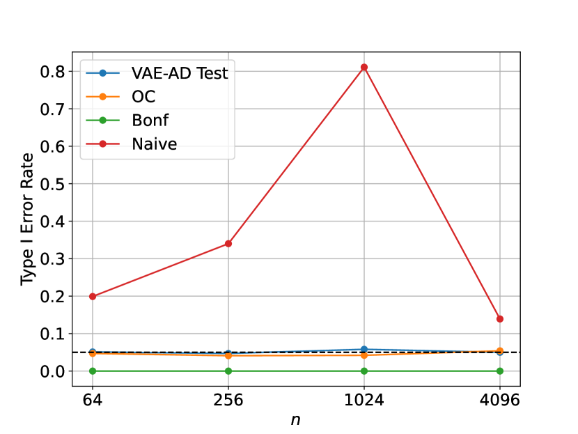
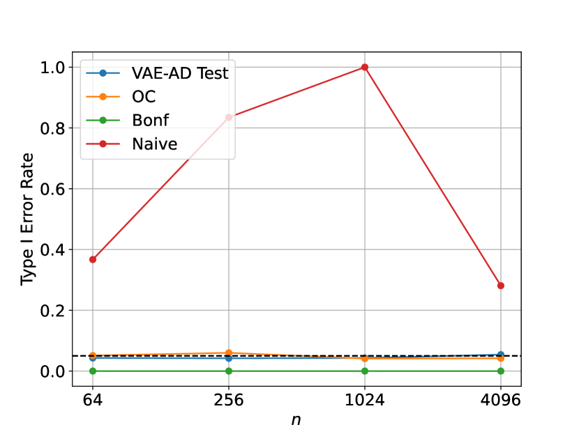
(a) Independence (b) Correlation

Figure 2: Type I error rate comparison

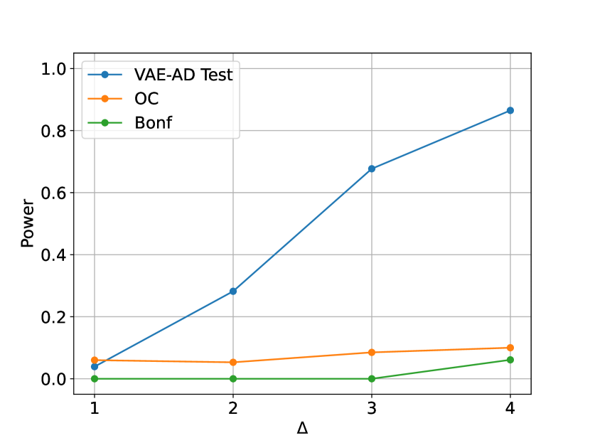
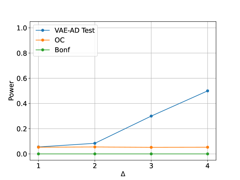
(a) Independence (b) Correlation

Figure 3: Power comparison

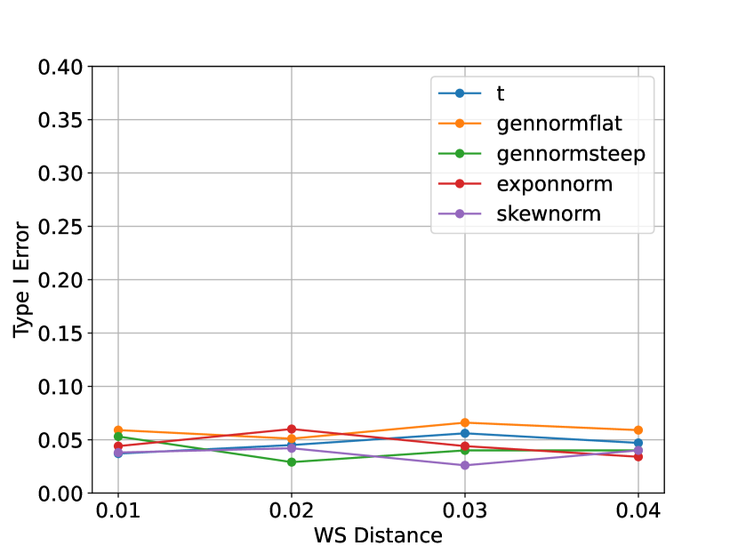
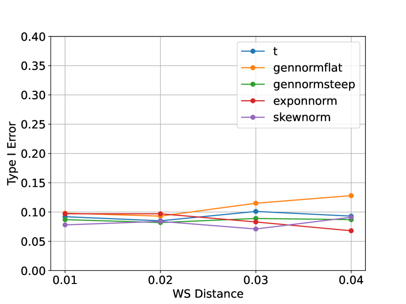
(a) $\alpha=0.05$. (b) $\alpha=0.10$.

Figure 4: Robustness of the proposed method.

Numerical results. The results of type I error rate and power are shown in Figs. 2 and 3, respectively. The VAE-AD Test, OC, and Bonf successfully controlled the type I error rate in the both cases of independence and correlation, whereas the naive method could not. Since the naive method failed to control the type I error, we no longer considered its power. The power of the VAE-AD Test was the highest among the methods that controlled the type I error. The Bonferroni method has the lowest power because it is conservative due to considering the huge number of all possible hypotheses. OC also has low power because it considers extra conditioning, which causes the loss of power.

Additionally, we confirm the robustness of the VAE-AD Test in terms of type I error control when the noise follows skew normal distribution, exponential normal distribution, generalized normal distribution with flat tails, and $t$ distribution. More details can be found in Appendix D. The results are shown in Fig. 4. Our method still maintains good performance in type I error rate control.

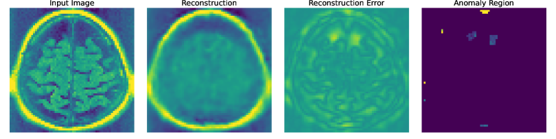
(a) $p_{\rm naive}=0.000,\;p_{\rm selective}=0.431$

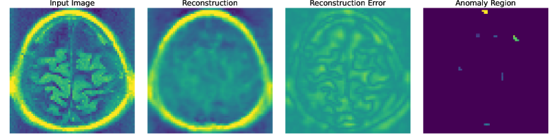
(b) $p_{\rm naive}=0.000,\;p_{\rm selective}=0.849$

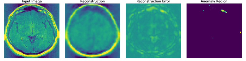
(c) $p_{\rm naive}=0.000,\;p_{\rm selective}=0.196$

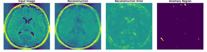
(d) $p_{\rm naive}=0.000,\;p_{\rm selective}=0.797$

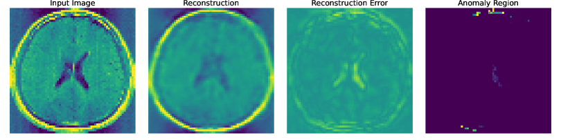
(e) $p_{\rm naive}=0.000,\;p_{\rm selective}=0.299$

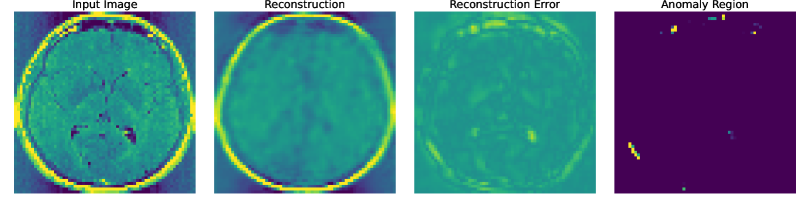
(f) $p_{\rm naive}=0.000,\;p_{\rm selective}=0.598$

Figure 5: Anomaly detection for images without tumor.

Real data experiments. We examined the brain image dataset extracted from Buda et al. (2019), which includes 939 and 941 images with and without tumors, respectively. The results of statistical testing for images without tumor and with tumor are presented in Figs. 5 and 6. The naive $p$-value is small even in cases where no tumor region exists in the image. This indicates that the naive $p$-value cannot be used to quantify the reliability of the result of anomaly detection using VAE. With the proposed selective $p$-values, we successfully identified false and true positive detections.

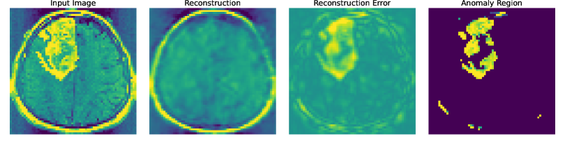
(a) $p_{\rm naive}=0.000,\;p_{\rm selective}=0.048$

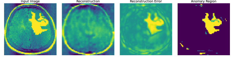
(b) $p_{\rm naive}=0.000,\;p_{\rm selective}=0.000$

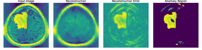
(c) $p_{\rm naive}=0.000,\;p_{\rm selective}=0.017$

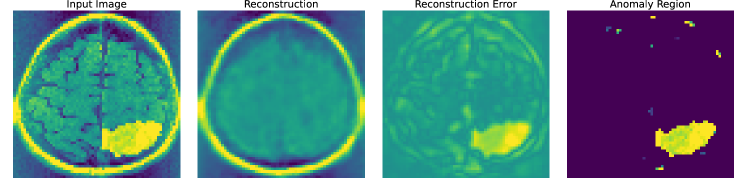
(d) $p_{\rm naive}=0.000,\;p_{\rm selective}=0.000$

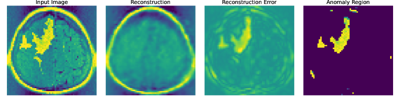
(e) $p_{\rm naive}=0.000,\;p_{\rm selective}=0.000$

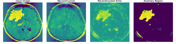
(f) $p_{\rm naive}=0.000,\;p_{\rm selective}=0.000$

Figure 6: Anormaly detection for images with tumor.

7 Conclusion

We proposed a novel setup of testing the results of VAE-AD and introduced a method to compute a valid $p$-value for conducting the statistical test. The experiments were conducted on both synthetic and real-world datasets to showcase the superior performance of the proposed method. We believe that this study stands as a significant step toward reliability of VAE-driven hypotheses.

Acknowledgements

This work was partially supported by MEXT KAKENHI (20H00601), JST CREST (JPMJCR21D3), JST Moonshot R&D (JPMJMS2033-05), JST AIP Acceleration Research (JPMJCR21U2), NEDO (JPNP18002, JPNP20006), and RIKEN Center for Advanced Intelligence Project.

Appendix A The details of VAE

We used the architecture of the VAE as shown in Figure 7 and set $m=10$ as a dimensionality of the latent space. We used ReLU as an activation function for the encoder and decoder. We generated 1000 images from $N(\bm{0},I_{n})$ as normal images and trained the VAE with these images, and used Adam [Kingma and Ba, 2017] as an optimizer.

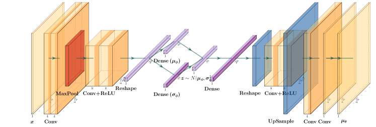
Figure 7: Architecture of the VAE.

Appendix B Proof of Theorem 4.1

Proof.

The theorem is based on the Lemma 3.1 in Chen and Bien [2019]. By the definition of the piecewise-assignment function, the conditional part, $\{M_{\bm{X}}=M_{\bm{x}}\}$ can be characterized as the union of polytopes,

$$\{M_{\bm{X}}=M_{\bm{x}}\}=\bigcup_{k:M_{k}=M_{\bm{x}}}P_{k}^{\mathcal{M}}.$$

By substituting $\bm{X}(Z)=\mathcal{Q}_{\bm{x}}+\Sigma\bm{\eta}(\bm{\eta}^{\top}\Sigma\bm{\eta})^{-1}Z$ into the polytopes $P_{k}^{M}$, we obtain the truncated intervals $\mathcal{Z}$ in the lemma. For the set $k$ such that $M_{k}=M_{\bm{x}}$, we have $\mathcal{Q}_{\bm{X}}\perp Z$ by orhtogonality of $\mathcal{Q}_{\bm{X}}$ and $\bm{\eta}$ and by the properties of the normal distribution. Hence, we obtain

$$Z\mid\{M_{\bm{X}}=M_{\bm{x}},\mathcal{Q}_{\bm{X}}=\mathcal{Q}_{\bm{x}}\} \stackrel{{\scriptstyle d}}{{=}}Z\mid\{Z\in\mathcal{Z},\mathcal{Q}_{\bm{X}}=\mathcal{Q}_{\bm{x}}\}$$

$$\stackrel{{\scriptstyle d}}{{=}}Z\mid\{Z\in\mathcal{Z}\}\;(\because\mathcal{Q}_{\bm{X}}\perp Z)$$

There is no randomness in $\mathcal{Z}$,

$$Z\mid\{M_{\bm{X}}=M_{\bm{x}},\mathcal{Q}_{\bm{X}}=\mathcal{Q}_{\bm{x}}\}\sim TN(\bm{\eta}^{\top}\bm{\mu},\bm{\eta}^{\top}\Sigma\bm{\eta};\mathcal{Z}).$$

∎

Appendix C The Details of auto-conditioning

This section demonstrates the auto-conditioning algorithm, utilized to compute the truncated intervals $[L_{k}^{\mathcal{A}},U_{k}^{\mathcal{A}}]$ and the corresponding anomaly region $A_{k}$ respect to the $z$ in Algorithm 1. The algorithm is introduced for the piecewise-assignment function, which is composed of piecewise-linear functions and a piecewise-assignment function.

It is conceptualized as a directed acyclic graph (DAG) that delineates the processing of input data, similar to a computational graph in auto-differentiation. In this graph, the nodes symbolize the piecewise-linear and piecewise-assignment functions, each with an input and output edge to represent the function compositions. It should be noted that the node such as $\bm{\mu}_{\bm{\phi}}$ and $\bm{\mu}_{\bm{\theta}}$, may replace the other DAG express the piecewise-linear/assignment function of the node since it can be represented as the composition and concatenation of array of simpler piecewise-linear/assignment functions. The level of simplicity for a function of a node can be determined based on what is most convenient for the implementation. A special node, representing the concatenation of two piecewise-linear functions, features two input edges and one output edge. Figure 8 shows the directed acyclic graph of the anomaly detection using VAE in Eq. (4).

Figure 8: The directed acyclic graph of the anomaly detection using VAE $\mathcal{A}:\mathbb{R}^{n}\rightarrow 2^{|n|}$ defined in Eq. (4). Circles represent the piecewise-linear functions and the piecewise-assignment function. The rectangle represents the concatenation of piecewise-linear functions. The edges represent the composition of piecewise-linear functions.

C.1 Update rules for the nodes of the piecewise-assignment functions

The computation of the interval $[L_{k}^{\mathcal{A}},L_{k}^{\mathcal{A}}]$ is defined in a recursive way. The output of the node $f:\mathbb{R}^{l}\rightarrow\mathbb{R}^{m}$ in the DAG are denoted as $\bm{a}_{f},\bm{b}_{f}\in\mathbb{R}^{m}$ and $L_{f},U_{f}\in\mathbb{R}$.

Update rule for the initial node.

At first, the output of the initial node $\bm{X}(z)$ of the directional graph denoted as $f_{0}$ for notational convention, are defined as $\bm{a}_{f_{0}}=\mathcal{Q}_{\bm{x}}$, $\bm{b}_{f_{0}}=\Sigma\bm{\eta}(\bm{\eta}^{\top}\Sigma\bm{\eta})^{-1}$, $L_{f_{0}}=-\infty$, and $U_{f_{0}}=\infty$. It should be noted here that $\bm{X}(z)=\bm{a}_{f_{0}}+\bm{b}_{f_{0}}z$ is the line appeared in the proof of Theorem 4.1 in Section B.

Update rule for the node of the piecewise-linear functions.

Let us consider the output for the node $g$ whose input is the output of the node $f$ in the DAG. The inputs of the $g$’s node  (i.e. output of node $f$) are denoted as $\bm{a}_{f},\bm{b}_{f},L_{f}$ and $U_{f}$. $\bm{a}_{f}$ is the summed point vector added in the piecewise-linear functions until reaching $f$, $\bm{b}_{f}$ is the direction vector corresponding to $z$, multiplied in the piecewise-linear functions until reaching to $f$. Then, the output of the piecewise-linear function $f$ is represented as $\bm{a}_{f}+\bm{b}_{f}z$. $L_{f}$ and $U_{f}$ are the lower and upper bounds of the interval obtained at the piecewise-linear function $f$. The output of the node $g$ is defined as follows: 1) Check the index $j$ such that the output of $f$ within the polytope of: $P_{j}^{g}\ni\bm{a}_{f}+\bm{b}_{f}z$. 2) Compute the point vector $\bm{a}_{g}$ and the direction vector $\bm{b}_{g}$ of the piecewise-linear function $g$ with the index $j$,

$$\bm{a}_{g}=\bm{\Psi}_{j}^{g}\bm{a}_{f}+\bm{\psi}_{j}^{g},\;\bm{b}_{g}=\bm{\Psi}_{j}^{g}\bm{b}_{f}.$$ (13)

3) Compute the lower and upper bounds of the interval $L_{g}$ and $U_{g}$ with the index $j$,

$$L=\max_{k:({\bm{\beta}^{g}_{j}})_{k}>0}\frac{({\bm{\alpha}^{g}_{j}})_{k}}{({\bm{\beta}^{g}_{j}})_{k}},\;U=\min_{k:({\bm{\beta}^{g}_{j}})_{k}<0}\frac{({\bm{\alpha}^{g}_{j}})_{k}}{({\bm{\beta}^{g}_{j}})_{k}},$$

where $\bm{\alpha}^{g}_{j}=\bm{\delta}^{g}_{j}-\bm{\Delta}^{g}_{j}\bm{a}_{f}$ and $\bm{\beta}^{f}_{j}=\bm{\Delta}^{g}_{j}\bm{b}_{f}$. 4) Take the intersection of the interval $[L_{f},U_{f}]\cap[L,U]$ as the interval $[L_{g},U_{g}]$ of the piecewise-assignment function $g$ as

$$L_{g}=\max(L_{f},L),\;U_{g}=\min(U_{f},U).$$

This update rule is obtained from the Lemma 2 in Miwa et al. [2023].

Update rule for the nodes of concatenation of two piecewise-linear functions.

Let us consider the concatenation node of two piecewise-linear functions $f$ and $g$ denoted as concat. Let the inputs of the node be $\bm{a}_{f},\bm{b}_{f},L_{f}$ and $U_{f}$ from the node $f$ and $\bm{a}_{g},\bm{b}_{g},L_{g}$ and $U_{g}$ from the node $g$. The output of the concatenation node, $\bm{a}_{\rm concat}$, $\bm{b}_{\rm concat}$, $L_{\rm concat}$ and $U_{\rm concat}$ are defined as follows: 1) Concatenate the vector outputs of nodes $f$ and $g$

$$\bm{a}_{\rm concat}=\begin{bmatrix}\bm{a}_{f}\\ \bm{a}_{g}\end{bmatrix},\;\bm{b}_{\rm concat}=\begin{bmatrix}\bm{b}_{f}\\ \bm{b}_{g}\end{bmatrix}.$$

2) Take intersection of the interval $[L_{f},U_{f}]\cap[L_{g},U_{g}]$ as

$$L_{\rm concat}=\max(L_{f},L_{g}),\;U_{\rm concat}=\min(U_{f},U_{g}).$$

Update rule for the final node.

At the final node $\Theta$ which is the piecewise-assignment function, it takes the same input as the node of piecewise-linear functions and outputs are the same except for the $\bm{a}_{\Theta}$ and $\bm{b}_{\Theta}$. 1) It computes the index $j$ such that the input falls into the polypotopes of $P_{j}^{\Theta}$. 2) Then, the anomaly region $A_{j}$ is obtained instead of Eq. (13) in the update rule for the node of piecewise-linear functions. 3) The computation of lower bounds $L_{\Theta}$ and the upper bounds $U_{\Theta}$ are the same as the update rule for the node of piecewise-linear functions. The output of the final node are the anomaly region $A_{j}$, the lower bounds $L_{\Theta}$ and the upper bounds $U_{\Theta}$.

Then, apply the above update rule to the directional graph of the piecewise-assignment function from the initial node $f_{0}$ to the final node $\Theta$. Consequently, the auto-conditioning algorithm computes the lower and upper bounds of the interval as the outputs of final node $L_{k}^{\mathcal{A}}=L_{\Theta},L_{k}^{\mathcal{A}}=L_{\Theta}$ and $A_{k}=A_{j}$.

C.2 Implementation

We implemented the auto-conditioning algorithm described above in Python using the tensorflow library. The codes construct the DAG of the piecewise-assignment function automatically from the trained Keras/tensorflow model. Then, we do not need further implementation to conduct CSI for each specific DNN model. This indicates that even if we change the architecture or adjust the hyper-parameters and retrain the DNN models, we can conduct the CSI without additional implementation.

Appendix D Experimental Details

Methods for comparison.

We compared our proposed method with the following methods:

$\bullet$ VAE-AD Test: our proposed method.

$\bullet$ OC: our proposed method conditioning on the only one polytope to which the observed image belongs $\bm{x}\in P_{k}^{\mathcal{A}}$. This method is computationally efficient; however, its power is low due to over-conditioning.

$\bullet$ Bonf: the number of all possible hypotheses are considered to account for the selection bias. The $p$-value is computed by $p_{\rm bonf}=\min(1,p_{naive}\times 2^{n})$

$\bullet$ Naive: the conventional method is used to compute the $p$-value.

Experiment for robustness.

We evaluate the robustness of our proposed methodology in terms of Type I error control, specifically under conditions where the noise distribution deviates from the Gaussian assumption. We investigate this robustness by applying our method across a range of non-Gaussian noise distributions, including:

$\bullet$ Skew normal distribution (skewnorm)

$\bullet$ Exponential normal distribution (exponorm)

$\bullet$ Generalized normal distribution with steep tails (gennormsteep)

$\bullet$ Generalized normal distribution with flat tails (gennomflat)

$\bullet$ Student’s $t$ distribution (t)

We commence our analysis by identifying noise distributions from the aforementioned list that have a 1-Wasserstein distance of $\{0.01,0.02,0.03,0.04\}$ relative to the standard normal distribution $N(0,1)$. Subsequently, we standardize these noise distributions to ensure a mean of 0 and a variance of 1. Setting the sample size to $n=256$, we generate 1000 samples from the selected distributions and apply hypothesis testing to each sample to obtain the Type I error rate. This process is conducted at significance levels $\alpha=\{0.05,0.10\}$. The results are shown in Figure 4. Our method still maintains good performance even when the assumption of Gaussian noise is violated.

More results on brain image dataset.

Additional results are shown in Figs. 9 and 10.

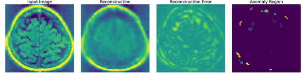
(a) $p_{\rm naive}=0.000,\;p_{\rm selective}=0.668$

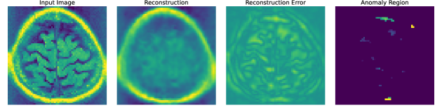
(b) $p_{\rm naive}=0.000,\;p_{\rm selective}=0.849$

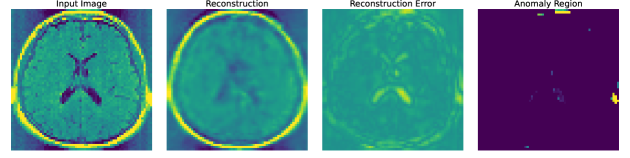
(c) $p_{\rm naive}=0.011,\;p_{\rm selective}=0.500$

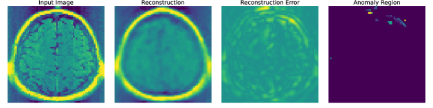
(d) $p_{\rm naive}=0.012,\;p_{\rm selective}=0.137$

Figure 9: Anomaly detection for image without tumor.

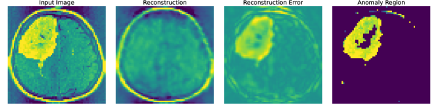
(a) $p_{\rm naive}=0.000,\;p_{\rm selective}=0.001$

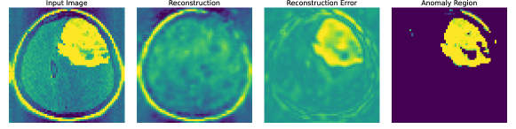
(b) $p_{\rm naive}=0.000,\;p_{\rm selective}=0.000$

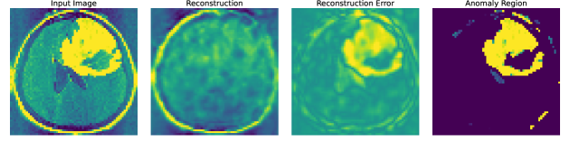
(c) $p_{\rm naive}=0.000,\;p_{\rm selective}=0.000$

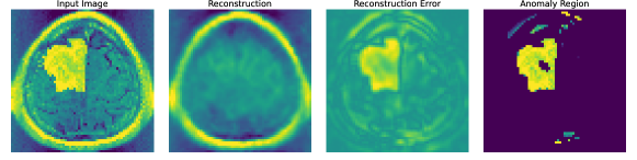
(d) $p_{\rm naive}=0.000,\;p_{\rm selective}=0.017$

Figure 10: Anormaly detection for image with tumor.

References

- Anonymous [2024a] Anonymous. Statistical test for generated hypotheses by diffusion models. Unpublished, 2024a.
- Anonymous [2024b] Anonymous. Statistical test for attention maps in vision transformers. Unpublished, 2024b.
- Baur et al. [2019] C. Baur, B. Wiestler, S. Albarqouni, and N. Navab. Deep Autoencoding Models for Unsupervised Anomaly Segmentation in Brain MR Images, page 161–169. Springer International Publishing, 2019. ISBN 9783030117238. doi: 10.1007/978-3-030-11723-8˙16. URL http://dx.doi.org/10.1007/978-3-030-11723-8_16.
- Baur et al. [2021] C. Baur, S. Denner, B. Wiestler, N. Navab, and S. Albarqouni. Autoencoders for unsupervised anomaly segmentation in brain mr images: A comparative study. Medical Image Analysis, 69:101952, 2021. ISSN 1361-8415. doi: https://doi.org/10.1016/j.media.2020.101952. URL https://www.sciencedirect.com/science/article/pii/S1361841520303169.
- Breiman [1992] L. Breiman. The little bootstrap and other methods for dimensionality selection in regression: X-fixed prediction error. Journal of the American Statistical Association, 87(419):738–754, 1992.
- Buda et al. [2019] M. Buda, A. Saha, and M. A. Mazurowski. Association of genomic subtypes of lower-grade gliomas with shape features automatically extracted by a deep learning algorithm. Computers in Biology and Medicine, 109:218–225, 2019. ISSN 0010-4825. doi: https://doi.org/10.1016/j.compbiomed.2019.05.002. URL https://www.sciencedirect.com/science/article/pii/S0010482519301520.
- Chalapathy and Chawla [2019] R. Chalapathy and S. Chawla. Deep learning for anomaly detection: A survey. arXiv preprint arXiv:1901.03407, 2019.
- Chen and Bien [2019] S. Chen and J. Bien. Valid inference corrected for outlier removal. Journal of Computational and Graphical Statistics, pages 1–12, 2019.
- Chen and Bien [2020] S. Chen and J. Bien. Valid inference corrected for outlier removal. Journal of Computational and Graphical Statistics, 29(2):323–334, 2020.
- Chen and Konukoglu [2018] X. Chen and E. Konukoglu. Unsupervised detection of lesions in brain MRI using constrained adversarial auto-encoders. In Medical Imaging with Deep Learning, 2018. URL https://openreview.net/forum?id=H1nGLZ2oG.
- Choi et al. [2017] Y. Choi, J. Taylor, and R. Tibshirani. Selecting the number of principal components: Estimation of the true rank of a noisy matrix. The Annals of Statistics, 45(6):2590–2617, 2017.
- Chow et al. [2020] J. K. Chow, Z. Su, J. Wu, P. S. Tan, X. Mao, and Y.-H. Wang. Anomaly detection of defects on concrete structures with the convolutional autoencoder. Advanced Engineering Informatics, 45:101105, 2020.
- Dehaene et al. [2020] D. Dehaene, O. Frigo, S. Combrexelle, and P. Eline. Iterative energy-based projection on a normal data manifold for anomaly localization, 2020.
- Duy et al. [2020] V. N. L. Duy, H. Toda, R. Sugiyama, and I. Takeuchi. Computing valid p-value for optimal changepoint by selective inference using dynamic programming. In Advances in Neural Information Processing Systems, 2020.
- Duy et al. [2022] V. N. L. Duy, S. Iwazaki, and I. Takeuchi. Quantifying statistical significance of neural network-based image segmentation by selective inference. Advances in Neural Information Processing Systems, 35:31627–31639, 2022.
- Fithian et al. [2015] W. Fithian, J. Taylor, R. Tibshirani, and R. Tibshirani. Selective sequential model selection. arXiv preprint arXiv:1512.02565, 2015.
- Gao et al. [2022] L. L. Gao, J. Bien, and D. Witten. Selective inference for hierarchical clustering. Journal of the American Statistical Association, pages 1–11, 2022.
- Jana et al. [2022] D. Jana, J. Patil, S. Herkal, S. Nagarajaiah, and L. Duenas-Osorio. Cnn and convolutional autoencoder (cae) based real-time sensor fault detection, localization, and correction. Mechanical Systems and Signal Processing, 169:108723, 2022.
- Kingma and Ba [2017] D. P. Kingma and J. Ba. Adam: A method for stochastic optimization, 2017.
- Kingma and Welling [2013] D. P. Kingma and M. Welling. Auto-encoding variational bayes. arXiv preprint arXiv:1312.6114, 2013.
- Le Duy and Takeuchi [2021] V. N. Le Duy and I. Takeuchi. Parametric programming approach for more powerful and general lasso selective inference. In International conference on artificial intelligence and statistics, pages 901–909. PMLR, 2021.
- Lee et al. [2015] J. D. Lee, Y. Sun, and J. E. Taylor. Evaluating the statistical significance of biclusters. Advances in neural information processing systems, 28, 2015.
- Lee et al. [2016] J. D. Lee, D. L. Sun, Y. Sun, and J. E. Taylor. Exact post-selection inference, with application to the lasso. The Annals of Statistics, 44(3):907–927, 2016.
- Loftus and Taylor [2014] J. R. Loftus and J. E. Taylor. A significance test for forward stepwise model selection. arXiv preprint arXiv:1405.3920, 2014.
- Lu and Xu [2018] Y. Lu and P. Xu. Anomaly detection for skin disease images using variational autoencoder. arXiv preprint arXiv:1807.01349, 2018.
- Miwa et al. [2023] D. Miwa, D. V. N. Le, and I. Takeuchi. Valid p-value for deep learning-driven salient region. In Proceedings of the 11th International Conference on Learning Representation, 2023.
- Pang et al. [2021] G. Pang, C. Shen, L. Cao, and A. V. D. Hengel. Deep learning for anomaly detection: A review. ACM computing surveys (CSUR), 54(2):1–38, 2021.
- Sugiyama et al. [2021] K. Sugiyama, V. N. Le Duy, and I. Takeuchi. More powerful and general selective inference for stepwise feature selection using homotopy method. In International Conference on Machine Learning, pages 9891–9901. PMLR, 2021.
- Suzumura et al. [2017] S. Suzumura, K. Nakagawa, Y. Umezu, K. Tsuda, and I. Takeuchi. Selective inference for sparse high-order interaction models. In Proceedings of the 34th International Conference on Machine Learning-Volume 70, pages 3338–3347. JMLR. org, 2017.
- Tanizaki et al. [2020] K. Tanizaki, N. Hashimoto, Y. Inatsu, H. Hontani, and I. Takeuchi. Computing valid p-values for image segmentation by selective inference. In Proceedings of the IEEE/CVF Conference on Computer Vision and Pattern Recognition, pages 9553–9562, 2020.
- Tao et al. [2022] X. Tao, X. Gong, X. Zhang, S. Yan, and C. Adak. Deep learning for unsupervised anomaly localization in industrial images: A survey. IEEE Transactions on Instrumentation and Measurement, 71:1–21, 2022. ISSN 1557-9662. doi: 10.1109/tim.2022.3196436. URL http://dx.doi.org/10.1109/TIM.2022.3196436.
- Taylor and Tibshirani [2015] J. Taylor and R. J. Tibshirani. Statistical learning and selective inference. Proceedings of the National Academy of Sciences, 112(25):7629–7634, 2015.
- Tibshirani et al. [2016] R. J. Tibshirani, J. Taylor, R. Lockhart, and R. Tibshirani. Exact post-selection inference for sequential regression procedures. Journal of the American Statistical Association, 111(514):600–620, 2016.
- Wang et al. [2020] X. Wang, Y. Du, S. Lin, P. Cui, Y. Shen, and Y. Yang. advae: A self-adversarial variational autoencoder with gaussian anomaly prior knowledge for anomaly detection. Knowledge-Based Systems, 190:105187, 2020. ISSN 0950-7051. doi: https://doi.org/10.1016/j.knosys.2019.105187. URL https://www.sciencedirect.com/science/article/pii/S0950705119305283.
- Zimmerer et al. [2019] D. Zimmerer, F. Isensee, J. Petersen, S. Kohl, and K. Maier-Hein. Unsupervised anomaly localization using variational auto-encoders, 2019.