Dynamical complex networks for understanding motility induced phase separation in Active Brownian Particles

Abstract

We investigate the dynamics of active Brownian particles (ABP) through a temporal complex network framework, focusing on degree probability distribution, average path length, and clusterization across Motility-Induced Phase Separation (MIPS) regions. In the single MIPS phase, particle encounters resemble a random graph. Transitioning toward the MIPS frontier introduces a non-power-law distribution, while the phase-separated region exhibits a double power-law distribution. Numerical analysis indicates a shift from random to power-law complex networks based on the system’s MIPS-phase position. In summary, our numerical and theoretical analysis reveals the phase transition of the system between two states and how this transition manifests itself in the complex network, showing an evident change between a random network and a network that tends to have scale-free behavior.

1 Introduction

Active Brownian Particles (ABP) serve as a valuable framework for investigating the non-equilibrium dynamics and statistical properties of self-propelled agents, whether they are living organisms or artificial entities [1, 2]. In contrast to passive Brownian particles studied in random diffusive systems, ABP offers a new dimension of complexity due to the inherent particle self-propulsion mechanisms. In particular, these active particles undergo a distinctive phase transition known as Motility-Induced Phase Separation (MIPS) [3, 4, 5, 6, 7]. This phase transition is related to the spontaneous separation between dilute (free-particles) and dense phases (cluster formation) [5, 8, 9]. This phase separation is a fascinating emergent phenomenon where particles collapse into clusters although natural repulsion forces are present. The exploration of ABP not only deepens our understanding of self-organization and emergent phenomena but also opens up promising avenues for harnessing their unique properties in various applications and technological advancements [10] and building a bridge between physical models and biological systems.

The complexity of ABP dynamics and its statistical properties offer novel opportunities for deeper complex network analysis to better understand the role of particle connections during the dynamics. The particle interaction or contact dynamic between particles within this system is still a significant topic of interest, where the effects of particle shape [6], inertia [11], hydrodynamic interactions [12, 6, 13, 14] and quorum sensing [15] among others has been studied numerically and analytically in the context of motility-induced clustering and motility-induced separation. In recent years agent-based-models such as ABP have been used to construct from particle direct physical contact the contagion dynamics on the top of compartmental ecological models [16, 8, 17], or from more complicated pathways where temporal networks has been used to track burstiness or clusterization in the system [18, 19, 20, 21]. In recent work, McDermott et al. unveil the time evolution hidden in the clustering effect during MIPS using machine learning [22], where they demonstrate different regimes close the phase separation.

In the last years, studies conducted by complex networks have been applied to many natural systems such as social interactions [23, 24, 25], seismology [26, 27, 28, 29], space plasmas [30, 31], or biological interactions[32, 33, 34, 35, 36], among others. The formalism of complex networks can show a non-trivial behavior in systems due to their geometrical and topological foundations [37, 38]. Throughout a complex network analysis, we can characterize and describe a physical system based on its topological properties. Thus, we can classify a complex network based on its structural organization of connections between nodes such as a random network [39], a scale-free network [40], or a small-world network [41], for example. Due to the random encounters between ABP, one can construct a temporally averaged network that allows us to analyze the dynamics in terms of the topology of such connections. This new approach may motivate new questions or characterize the phase transition (MIPS) using the language of complex networks.

In this work, we carry out a new manner of analyzing ABP using complex networks: we build a time-averaged network with the time evolution of a system of ABP, and we follow the changes in the topological features of the complex network through the degree distribution ($P(k)$), the clustering coefficient ($\bar{C}$) and the average path length ($l_{G}$). Our approach suggests that a random graph can characterize the dilute phase while a double power law distribution describes the MIPS region.

2 Active Brownian Particles (ABP) and motility-phase-separation

We consider $N$ self-propelled disk-like particles with position vectors $\mathbf{r}_{i}(t)=[x_{i}(t),y_{i}(t)]$ (center of the disk) and orientation vectors $\hat{\mathbf{u}}_{i}(t)=[\cos\theta_{i}(t),\sin\theta_{i}(t)]$ that obey overdamped Langevin dynamics in a flat 2D surface,

$$\dot{\mathbf{r}}_{i} = u_{0}\hat{\mathbf{u}}_{i}(t)+\bm{\xi}_{i,T}(t)/\gamma_{T}-(1/\gamma_{T})\nabla_{\mathbf{r}_{i}}U,$$ (1)

$$\dot{\hat{\mathbf{u}}}_{i} = (1/\gamma_{R})\bm{\xi}_{i,R}(t)\times\hat{\mathbf{u}}_{i}$$ (2)

where $\gamma_{T},\gamma_{R}$ are the Stokes friction coefficients associated with translation (T) and rotation (R) in the $x-y$ plane, respectively, $u_{0}$ represents the self-propelled velocity with constant magnitude see Figure 1. Also, in Eqs.(1) and (2), $\bm{\xi}_{T}(t)$ and $\bm{\xi}_{R}(t)$ are, respectively, the translational and rotational, Gaussian, white noises with zero mean, $\langle\bm{\xi}_{T}(t)\rangle=\langle\bm{\xi}_{R}(t)\rangle=\mathbf{0}$, and time correlation $\langle\bm{\xi}_{T}(t_{1})\bm{\xi}_{T}(t_{2})\rangle=D_{T}\delta(t_{1}-t_{2})$ and $\langle\bm{\xi}_{R}(t_{1})\bm{\xi}_{R}(t_{2})\rangle=D_{R}\delta(t_{1}-t_{2})$, where we can define $D_{T}$ and $D_{R}$ as the translation and rotation diffusion parameters. Finally, in Eq.(1), $U$ corresponds to the summation over steric interactions between particles at time $t$,

$$U=\sum_{i\neq j}U_{\text{WCA}}(\mathbf{r}_{i},\mathbf{r}_{j})$$ (3)

with $\mathbf{r}_{j}$ is the position of the $j-$th particle, and $U_{\text{WCA}}$ is the Weeks-Chandler-Andersen (WCA) pair potential

$$U_{\text{WCA}}(\mathbf{r}_{i},\mathbf{r}_{j})=\left\{\begin{array}[]{cc}\displaystyle{4\varepsilon\left[\left(\frac{\sigma}{r_{ij}}\right)^{12}-\left(\frac{\sigma}{r_{ij}}\right)^{6}\right]}&r_{ij}\leq C_{r}\\ 0&\mbox{otherwise}\end{array}\right.$$ (4)

with $r_{ij}=|\mathbf{r}_{i}-\mathbf{r}_{j}|$ is the distance between particles, $\sigma$ the particle diameter, $C_{r}=2^{1/6}\sigma\approx 1.1225\sigma$ is defined here as the contact radius, and $\varepsilon$ is the energy interaction strength between particles. We set $\varepsilon=3$ during our simulations unless we stated otherwise.

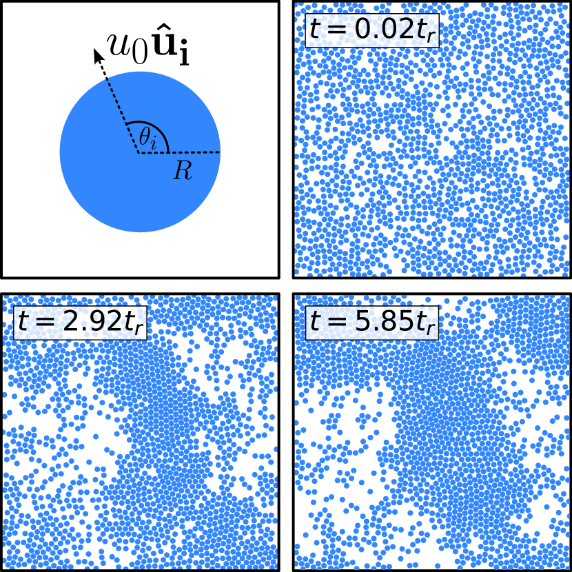
Figure 1: Time evolution for a system of active Brownian particles exhibiting Motility-induced phase separation: In the top-left, a single ABP is shown with orientation vector $\hat{u}_{i}$ and radius $R$. The time evolution is shown at three different times, showing a transition from a single phase in $t=0.02t_{r}$ and two coexisting phases in $t=5.85t_{r}$, at $\text{Pe}=140$ and $\phi=0.5$, with $L=100$ and $t_{r}=1/D_{R}$.

In this study, we conducted numerical simulations involving a collection of ABP moving within a square of area $L\times L$. Here, it is important to introduce the two dimensionless numbers to characterize different regimes. First, we introduce the packing fraction as $\phi=N\pi(\sigma/2)^{2}/L^{2}$, which relates the ratio between the area covered by the $N$ Active Brownian Particles with radius $\sigma/2$ with respect to the total available area. When the packing fraction increases, the high density allows clusters to be formed. In addition, these ABP systems exhibit a characteristic persistent motion reminiscent of a run-and-tumble state observed in self-phoretic systems and bacterial suspensions [42, 43, 14, 7]. The persistence time is defined as $t_{p}=\sigma/u_{0}$, while the memory kernel associated with tumble states is characterized by $t_{r}=1/D_{R}$. Since ABP can explore the available space through diffusion, it is natural to define $t_{r}$ as the relevant time scale of the problem. Second, we introduce the Péclet number $\text{Pe}=t_{r}/t_{p}=u_{0}t_{r}/\sigma$, which relates the ratio between diffusion and persistent times in transport phenomena. When the Péclet number is large, we have that ABP are persistent compared to diffusion. The latter is relevant for cluster formation since the minimal cluster for disk-shaped particles is formed with three persistent disks forming an equilateral triangle.

The interplay between steric interactions causing the blocking of persistent motion and an increased probability of collision due to elevated concentrations $\phi$ and particle activities $u_{0}$ leads to a fascinating phenomenon known as motility-induced phase separation (MIPS) [6, 5]. The system starts with a homogeneous particle distribution and orientations at $t=0$ exhibiting a single-phase behavior (or fluid-like state [44]), which physically describes ABP randomly moving without particle agglomeration. However, if the packing fraction and Péclet number are larger than some critical values, the system evolves into a two-phase state represented by a solid and gas phase, as illustrated in Figure 1. In this phase, particles agglomerate, and cluster formation becomes an emergent phenomenon.

An analytical alternative to represent this phase separation is using the separation kinetic function $f_{c}$, which reproduces the phase separation map in terms of the packing fraction, the Péclet number, and the average total number of particles lost per escape event $\kappa$ [4]

$$f_{c}=\frac{4\phi\text{Pe}-3\pi^{2}\kappa}{4\phi\text{Pe}-6\sqrt{3}\pi\kappa\phi}$$ (5)

In Fig. 2, we analytically reproduced the phase diagram in terms of the packing fraction and the Péclet number using $\kappa=4.7$ as a fit parameter [4]. The pairs $(\text{Pe},\phi)$ studied in this work are represented by the white dots of Fig. 2. For $f_{c}=0$, we can say that the system is in the single-phase, while for $f_{c}\neq 0$, the system undergoes a phase transition to the two-phase state. The system is considered steady when the phase separation shows a bimodal probability distribution for different local packing fractions [4, 5]. Despite extensive studies on phase separation in various contexts, machine learning has recently investigated the time evolution during phase separation, revealing different transition regimes [22]. In this work, we aim to study the time evolution by generating a temporal averaged network during the phase transition.

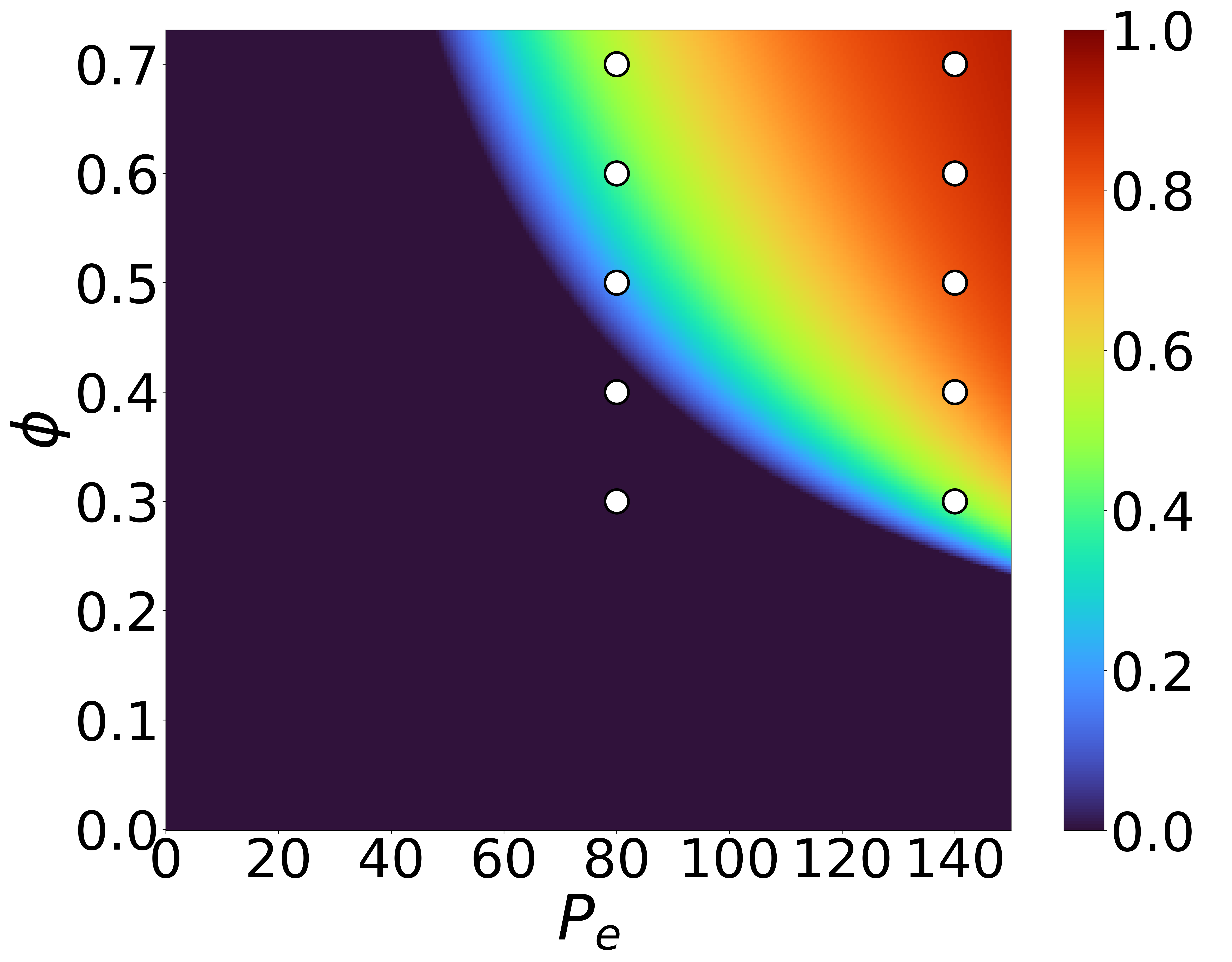
Figure 2: An analytical representation for the phase diagram in the $\text{Pe}-\phi$ plane plotted from the analytical model using Eq. 5, with $\kappa=4.7$. The white dots represent the pairs $(\text{Pe},\phi)$ parameters studied across this work.

2.1 Simulation methods and parameters

We employed standard Brownian dynamics methods to numerically solve the governing Eqs.(1) and (2) for $N\in[955,1274,1592,1910,2229]$ particles within a simulation box with a length of $L=100$ and periodic boundary conditions. We ran $20$ ensembles for each set of parameters, initiating simulations with random initial particle positions and orientations.

The relevant length scale in the system is the particle radius $R$, serving as the unit of length. Additionally, we adopted $t_{r}$ as the unit of time. The equations of motion, Eqs.(1) and (2), were integrated with a time step of $\Delta t=3\times 10^{-5}t_{r}$, and simulation times were set to $T=12t_{r}$. Two dimensionless values parameterize the system: the packing fraction $\phi$ and the Péclet number, which are varied in the intervals $\phi\in[0.3-0.7]$ and $\text{Pe}\in[80,140]$, respectively (see Fig. 2). We maintain a constant rotational diffusion coefficient $D_{R}=0.15$, translation diffusion coefficient $D_{T}=0.2$, and diameter $\sigma=2R$ with $R=1$.

3 Complex Networks for ABP

A network is defined as a group of nodes connected between them by edges. The connections between nodes could be directed or undirected. In this case, the nodes are determined by each ABP, and the interaction between particles defines the connections: two nodes (particles) are connected when their centers are inside the interaction region defined by the contact radius $C_{r}$ (see WCA potential in Eq. (4)). We build a time network by following the dynamics of the particle connections in a specific time window.

To have enough statistics, we define a window with sixty data points, and we count the connections between nodes each time; if two nodes are connected only once in a one-time step or if two nodes are connected along the sixty steps, the value of the connections in the adjacency matrix is one in that time window. We move the window to the next time window’s center and repeat the same procedure, as shown schematically in Fig. 3.

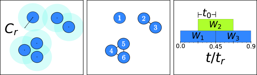
Figure 3: From left to right: A scheme for particle encounters when a pair interaction occurs. The blurred area represents the interaction region with radius $C_{r}$. Particles (nodes) generate a link if their centers enter each other’s interaction region, as shown in the middle panel. A representation of the time evolution for the network formation, with time windows of length $W=0.45t_{r}$ and overlap $t_{0}=0.225t_{r}$ between two consecutive windows.

3.1 Adjacency matrix

In order to analyze the system, we first create the adjacency matrix $A$, which is used to represent the network. Using the distance $r_{ij}=|\mathbf{r}_{i}-\mathbf{r}_{j}|$ between the centers of two particles, we can establish the value of $A_{ij}$ which represents the connections between these particles. If $r_{ij}\leq C_{r}$, we set $A_{ij}=A_{ji}=1$; otherwise, $A_{ij}=0$. If $A_{ij}=A_{ji}=1$ it means that two nodes (particles) are connected between them, and the complex network built is undirected. Within time windows of length $W=0.45t_{r}$ and using an overlapping time $t_{0}=0.225t_{r}$, a link is established only upon the first interaction between two particles. The latter means that each network accounts for unique particle encounters within the time window. From the adjacency matrix, we can compute all the necessary properties of the network. We will focus on calculating the degree distribution, network average clustering coefficient, and average path length.

3.2 Degree distribution

The degree $deg(p_{i})$ of each particle $p_{i}$ is the number of connections of a node, and it can be computed by summing over the corresponding column or row of the adjacency matrix:

$$deg(p_{i})=\sum_{j=1}^{N}A_{ij}=\sum_{j=1}^{N}A_{ji},$$ (6)

and the degree distribution is defined by

$$P(k)=\frac{n_{k}}{N},$$ (7)

which is directly obtained from simulations. Here $n_{k}$ is the total number of particles with degree $k$, and $N$ is the number of particles in the system. Depending on the topology of the complex network, the degree distribution could be binomial (random graphs), power-law (scale-free), among others. In this work, we shall discuss the role of the Gaussian distribution and double power law models in the context of MIPS.

3.3 Network average clustering coefficient

The clustering coefficient $C_{i}$ of each particle is a measure of the tendency to form clusters of this node, and it is defined by

$$C_{i}=\frac{1}{k_{i}(k_{i}-1)}\sum_{j,k}A_{ij}A_{jk}A_{ki},$$ (8)

where $A$ is the adjacency matrix, and $k_{i}$ is the degree of the particle. From this, we can calculate the network average clustering coefficient $\bar{C}$, which is the trend of the network to form clusters, and it is defined by

$$\bar{C}=\frac{1}{N}\sum_{i=1}^{N}C_{i},\quad\quad 0\leq\bar{C}\leq 1.$$ (9)

3.4 Average path length

The average path length is the rate between the shortest number of steps between two nodes and the shortest paths between all the pairs of nodes, and it is defined by [45],

$$l_{G}=\frac{1}{N(N-1)}\sum_{i\neq j}d(v_{i},v_{j}).$$ (10)

Here, $d(v_{i},v_{j})$ is the shortest distance between two vertices $v_{i}$ and $v_{j}$, where $v_{i,j}$ are nodes of the graph.

4 Results and Discussion

We studied three different regimes of the ABP according to the phase diagram of Fig. 2: (i) one-phase (violet), (ii) transient phase (blue-green), and (iii) two-phase (orange-red). As discussed in the following sections, these three regions will exhibit different topological properties, which are not reported in the literature to the best of our knowledge.

4.1 One-phase region: Random Graph

In the one-phase region (violet in Fig. 2), we found that the random motion of ABP can be characterized by a Gaussian function for the degree distribution

$$P^{\rm G}(k)={\frac{1}{\sigma_{\rm st}\sqrt{2\pi}}}\mbox{exp}\left[-\frac{1}{2}\left(\frac{k-\mu}{\sigma_{\rm st}}\right)^{2}\right],$$ (11)

where $\sigma_{\rm st}$ is the standard deviation, and $\mu$ is the average number of unique encounters of particles in a time window $W$. We have a dilute system for packing fraction numbers $\phi<0.4$, which allows us to analyze the average behavior of the ABP system using the kinetic theory of gases. As explained in Ref. [16], in an active media with $N$ moving particles in a dilute system, the mean free path is $\lambda=\sqrt{2}u_{0}\tau_{c}$, where $\tau_{c}$ is the mean time between encounters. During a time interval $\tau_{c}$, we can establish the probability constraint $p_{c}=A_{\rm sw}/L^{2}\approx 1$, where $A_{\rm sw}=N(2\lambda a+\pi a^{2})$ is the total area swept area of the $N$ particles, and $L^{2}$ is the available area. From this argument, it follows that $\lambda=(\pi/4)\phi^{-1}(1-\phi)\sigma=\sqrt{2}u_{0}\tau_{c}$. Then, the average number of encounters can be estimated as $\mu=W/\tau_{c}$, since, on average (by definition), particles have one encounter in the time interval $\tau_{c}$. We found:

$$\mu(\phi,\text{Pe})={4\sqrt{2}\over\pi}\left({\phi\over 1-\phi}\right)WD_{R}\text{Pe},$$ (12)

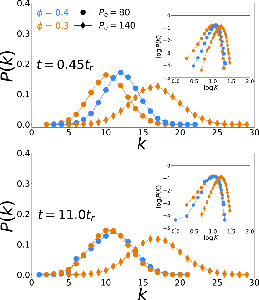
Figure 4: Degree distribution $P(k)$ for systems in the one-phase region at $\text{Pe}=80$ (circles) and $\text{Pe}=140$ (diamonds) at time $t=0.45t_{r}$ (top) and at $t=11.0t_{r}$ (bottom). The distributions show a Gaussian tendency; each system exhibits distinct mean and standard deviation values. Note that all systems maintain a Gaussian distribution, and only the system at $\phi=0.4$ shows a change over time. Both insets (top and bottom) show the $\log-\log$ plot of the systems at the respective time.

where $W=0.45t_{r}$ is fixed for $D_{R}=0.15$. In Fig. 4, we illustrate the evolution of the degree distribution $P(k)$ measured from Eqs. 6 and 7 for a system at two time lapses, $t=0.45t_{r}$ and $t=11.0t_{r}$. Two Péclet numbers are considered: $\text{Pe}=80$ represented by circles and $\text{Pe}=140$ represented by diamonds. Different packing fractions are depicted with orange and blue colors, corresponding to $\phi=0.3$ and $\phi=0.4$, respectively. Most importantly, using our model given in Eq. 12, we obtain $\mu(\phi=0.3,\text{Pe}=80)\approx 10.3$ and $\mu(\phi=0.3,\text{Pe}=140)\approx 16.2$, whose numerical values are close to those obtained by simulations ($10.51$ and $16.75$), see Fig. 5. This simple model can give good estimations of the central value of the Gaussian distribution $P^{\rm G}(k)$ given in equation 11, which is valid for the one-phase region.

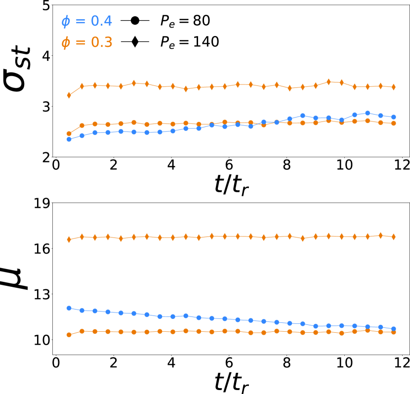
Figure 5: Standard deviation $\sigma_{st}$ (top) and mean $\mu$ (bottom) values over time of Gaussian fits for the degree distribution of systems in the one-phase region (Fig. 4). Both $\sigma_{st}$ and $\mu$ remain virtually constant over time and only the mean for the system at $\phi=0.4$ shows an appreciable decrease.

4.2 Transient Region: Hybrid phase

We define the transient region as the intermediate phase between the one-phase and two-phase regions (blue-green in Fig. 2). Since it is an intermediate phase, it is expected to have a degree of distribution with a hybrid behavior. Physically and analyzing our numerical simulations, we note that in this regime, small clusters composed of three disks (triangular arrangement) appear and eventually break because of the persistent ABP motion. In Fig. 6, we observe the degree distribution, average path length ($l_{G}$), and average clustering coefficient ($\bar{C}$) at times $t=0.45t_{r}$ and $t=11t_{r}$. Interestingly, the initially random graph (Gaussian distribution) evolves to a hybrid distribution with two components (Gaussian and power law). This hybrid behavior tells us that the system is trying to evolve from a random to a scale-free graph, but the values for the packing fraction and Péclet are not large enough. Moreover, at $t=11t_{r}$, the system does not reach the steady state, which is not the case for the one-phase and two-phase regions. The latter tells us that this hybrid phase is more complex to analyze regarding its geometrical and topological properties since the system remains out of equilibrium.

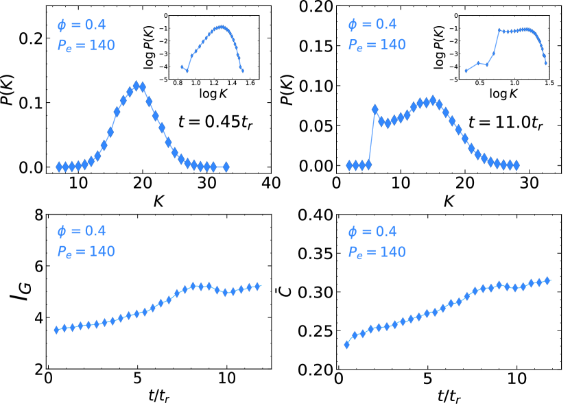
Figure 6: Top: Degree distribution for the case at $\text{Pe},\phi=80,0.4$ at the initial time $t=0.45t_{r}$ (right) and time $t=11.0t_{r}$ (left). The inset shows the same data plotted in $\log{}-\log{}$. Bottom: Average path length (left ) and average clustering coefficient (left) over time of the system. Both show an increasing behavior over time until $\approx 8t_{r}$.

4.3 Two-phase region: Phase separation

At more significant packing fractions and Péclet numbers, i.e., $\phi\geq 0.5$ and $\mbox{Pe}\geq 80$, the system enters the inner region of Fig. 2, where MIPS is manifested. From the point of view of the ABP, as time evolves, the initially random distribution (liquid-like state) evolves to a state where a gas-like and a solid-like phase cohabit in the system (green-red regions in Fig. 2). In terms of the complex network, the degree distribution of the system evolves from a Gaussian distribution at short times ($t=0.45t_{r}$) towards a double power law distribution for larger times ($t\geq 11t_{r}$); see Fig. 7(a)(b). Notably, when the degree distribution is plotted in the log-log scale, two slopes adequately describe the distribution $P(k)$, see Fig. 7(c)(d). This double power law distribution has the form

$$P(k>K)\sim\left\{\begin{array}[]{cr}k^{-\gamma_{1}},&k<k_{c}\\ k^{-\gamma_{2}},&k\geq k_{c}\end{array}\right.,$$ (13)

where $K=6$, $k_{c}\in[13-17]$ is the critical degree and $(\gamma_{1},\gamma_{2})$ are the critical exponents. The value $K=6$ is connected with the 2D disk packing problem, where each disk has exactly six nearest neighbors in an ideal cluster and corresponds to the peak of $P(k)$, see Fig. 7(b). Moreover, the critical values for $k_{c}$ depend on the clustering coefficient and Péclet number. The first slope $\gamma_{1}$ (red dashed line of Fig. 7) changes from values close to $1.5$ at $\phi=0.5$ towards values close to $3.7$ at $\phi=0.7$. The second slope $\gamma_{2}$ (black dashed lines) varies from values close to $12$ to $17$. In summary, we obtain $\gamma_{1}\approx(1.5-3.7)$ and $\gamma_{2}\approx(12-17)$, and therefore $\gamma_{1}<\gamma_{2}$ in our ABP model. In Table 1, we compare our results with different systems that exhibit a double power law distribution.

Physically, the $\gamma_{1}$ exponent is related to the solid cluster appearance where the degree number has a peak at $k=K$ ($\mbox{log}_{10}(6)\approx 0.78$). To better understand this, we plot the time evolution in Fig. 8, where it is clear that the slope value and, therefore, the cluster solid-like region is determined strongly by the system packing fraction $\phi$. On the contrary, the $\gamma_{2}$ exponent is related to less probable encounters related to the gas region, and we will not delve into that aspect.

The temporal behavior of both curves is shown in Fig. 8 ($\gamma_{1}$) and ($\gamma_{2}$). We note that $\gamma_{1}$ is more stable over time, and the packing fraction dominates its steady value in some inverse relation. On the contrary, $\gamma_{2}$ shows more oscillations, which can be explained because the clustering formation is unstable for the values of $(\phi,\mbox{Pe})$.

Table 1: Comparison between critical exponents for the double power law distribution in different models. Here, we are using the acronyms CAN = Chinese Airline Network, ABP = Active Brownian Particles, and MIPS = Motolity-Induced Phase Separation.

System	Network	$\gamma_{1}$	$\gamma_{2}$
or Data	(nodes, edges)	approx.	approx.
CAN Data [46]	(airports,flights)	$0.41-0.45$	$4.16-4.54$
US Flight Network Data [47]	(airports,flights)	$0.56-0.57$	$3.27-3.41$
Evolution of CAN [48]	(airports,flights)	$0.46-0.52$	$2.1-2.7$
Evolution of CAN [49]	(airports,flights)	$0.49$	$2.63$
Language model [50]	(words, connected words)	$3/2$	$2$
Homer’s Odyssey Data [51]	(words, connected words)	$0.76$	$1.19$
ABP (our work)	(particles, interacting particles)	$1.5-3.7$	$12-17$

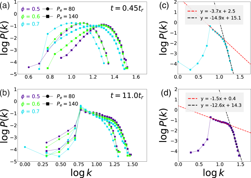
Figure 7: Degree distribution for phase-separated systems. (a) $\log{}-\log{}$ plot shows a clear Gaussian distributions at time $t=0.45t_{r}$. (b) degree distribution at $t=11.0t_{r}$ shows an evolution in the distribution where the degree $k=6$ for each curve is the one with the highest probability. Figures (c) and (d) show two distributions of the figure (b) zoomed in at $\text{Pe},\phi=(80,0.7)$ and $\text{Pe},\phi=(140,0.5)$ respectively, where the red and black dashed lines are the best linear fit for the first and second power law decay respectively for each distribution.

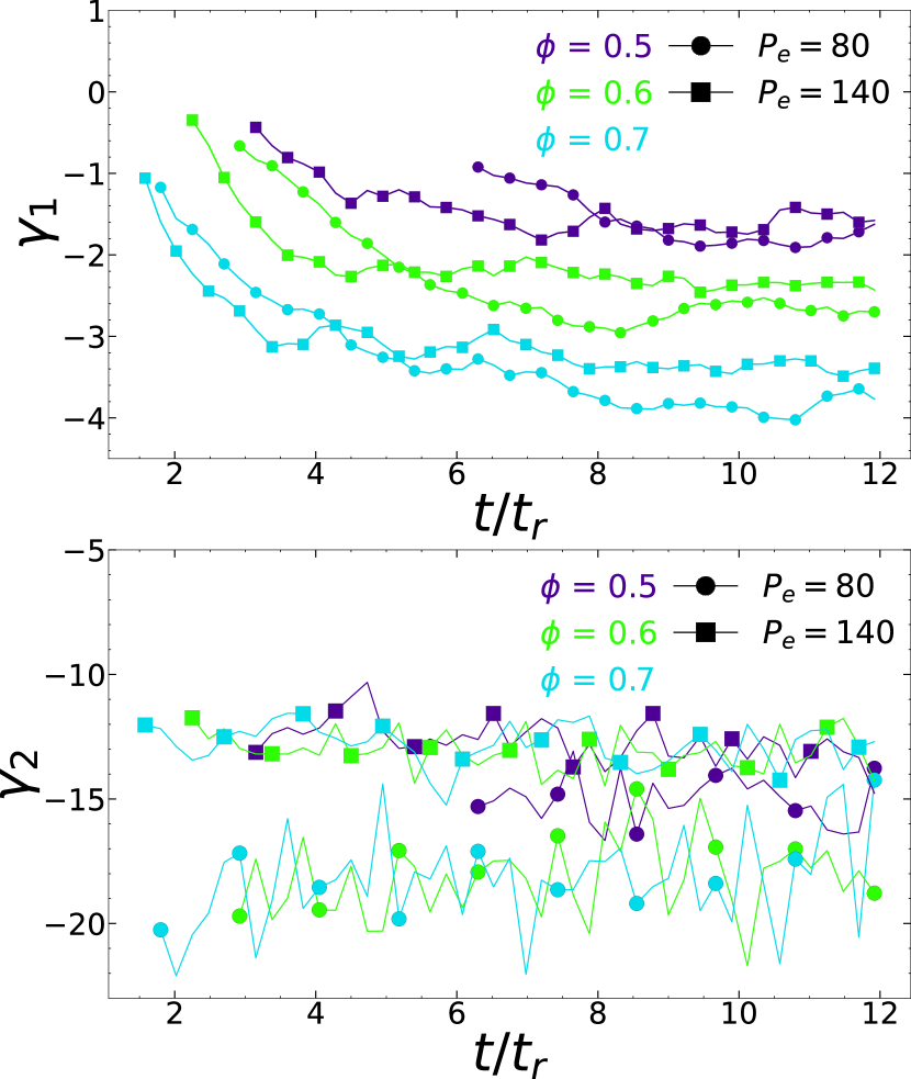
Figure 8: Slopes of the power law decay in the degree distribution for phase-separated systems. The initial data point occurs when the degree $k=6$ has the highest probability, indicating distinct curves for each system. Consequently, we observe different transition times. Notably, around $t\approx 8t_{r}$, the value of $\gamma_{1}$ (top) stabilizes consistently across all systems. In contrast, the values for the second slope, $\gamma_{2}$ (bottom), appear noisy and do not seem to stabilize.

4.3.1 Role of the average clustering coefficient

We can characterize this phase separation using the network average clustering coefficient $\bar{C}$ given in Eq. 9. In Fig. 9, we plot $\bar{C}$ as a function of time for different values of the packing fraction and Péclet number for the frontier and inner regions of the phase diagram illustrated in Fig. 2. To better understand the observed values of $\bar{C}$, we can elaborate a simple theoretical analysis. The clustering coefficient can be computed as $C=\lambda_{G}(v)/\tau_{G}(v)$, where $\lambda_{G}(v)$ is the number of triangles with one vertex on $v$ and $\tau_{G}(v)$ is the number of triples with one vertex on $v$ ($v$ is a vertex of the graph $G$). For a simple hexagonal cluster composed of seven particles (see inset of Fig. 10 (left)), we can calculate the clustering coefficient for one particle inside the cluster ($C_{i}$) and one particle in the border ($C_{b}$). Using this reasoning, we obtain $C_{i}=6/15=0.4$ and $C_{b}=2/3\approx 0.6667$. Let be $\bar{C}_{hex,N_{r}}$ the average clustering coefficient for a hexagonal arrangement with $N_{r}$ concentric hexagonal rings. For $N_{r}$ hexagonal rings, we have $6N_{r}$ particles in the border and $1+3N_{r}(N_{r}+1)$ particles in total. Therefore, the fraction of particles in the border and inside the cluster are $f_{b}(N_{r})=6N_{r}/(1+3N_{r}(N_{r}+1))$ and $f_{i}=(1+3N_{r}(N_{r}-1))/(1+3N_{r}(N_{r}+1))$, respectively. Thus, we can define the average clustering coefficient as,

$$\bar{C}_{hex,N_{r}}=f_{b}(N_{r})C_{b}+f_{i}(N_{r})C_{i}={2\over 15}\left[5-2f_{i}(N_{r})\right],$$ (14)

where we have used $f_{b}+f_{i}=1$. For instance, for $N_{r}=1$ (seven particles) we get $\bar{C}_{hex,7}=(1/7)C_{m}+(6/7)C_{b}\approx 0.6286$ (first value of Fig. 10 (left)). However, as one increases the fractions of particles inside the cluster ($f_{i}\rightarrow 1$), we get $\bar{C}_{hex,N_{r}}\rightarrow C_{i}=0.4$ (asymptotic value of Fig. 10 (left)). Also, it is important to mention that three disks forming a minimal cluster have an average cluster coefficient $\bar{C}=1$ (maximum value).

In Fig. 9, we note that in the frontier region of the MIPS phase diagram ($\phi=\{0.3,0.4\}$ and Pe $=\{80,140\}$), where small triangular clusters randomly appear, we observe $0.2\lesssim\bar{C}\lesssim 0.35$, and we associate these values for very low probability events (probabilities $\sim(0.2-0.35)$) of forming small triangular clusters. However, as we enter the inner region of the MIPS phase diagram ($\phi=\{0.5,0.6,0.7\}$ and Pe $=\{80.140\}$), finite hexagonal clusters are dominant, explaining the observed values $0.35\lesssim\bar{C}\lesssim 0.42$ at large times oscillates around $0.4$. A steady state value $\bar{C}\approx 0.35$ can be explained by the fact that a perfect hexagonal cluster with a clustering coefficient of 0.4 can be penalized by the fraction of particles with respect to the total number of particles. A value $\bar{C}\approx 0.42$ can be understood as the reference value 0.4 with a small contribution of small triangular clusters.

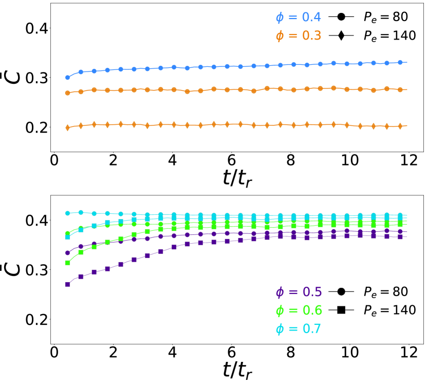
Figure 9: Top: Network average clustering coefficient for systems in the frontier region (top) and the inner region (bottom). The values for $\bar{C}$ for one-phased systems(top) at $\phi=0.3$ have virtually no change over time and slowly increase at $\phi=0.4$. In contrast, $\bar{C}$ for the two-phased systems increases rapidly at first and then stabilizes around $t=8t_{r}$, showing a tendency to $\bar{C}=0.4$.

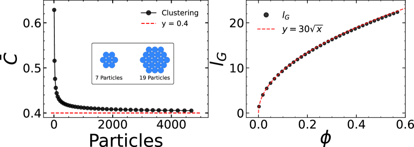
Figure 10: Left: Network average clustering coefficient of identical circles in a hexagonal packing arrangement, using $C_{r}=2^{1/6}\sigma$ ( black circles). $\bar{C}$ approaches asymptotically to $0.4$ (dashed red line), which is the value of the clustering coefficient of the center particle in the seven-particle arrangement (inset). Right: Average path length for the same hexagonal packing arrangement as a function of the packing fraction $\phi$ (black circles). We see that $l_{G}$ grows as $30\sqrt{\phi}$ (red dashed line) and could represent an upper bound with respect to $\phi$ for clustered ABP systems.

4.3.2 Role of the average path length

The average path length defined in Eq. 10 was measured for both regions, the frontier and inner region. In Fig. 11, we observe the time evolution for the network average path length in the case of a system with a single phase characterized by a Gaussian degree distribution $l_{G}$ has a constant value for different Pe numbers, meanwhile on the transient region for $\phi=0.4$ and Pe=$80$ the value increases slowly not reaching a constant value see blue dots in Figure 11.

In Fig. 10, we can observe a particular scaling for the average path length. In the ideal case (perfect hexagonal clusters with $N$ particles), we note that $l_{G}=30\phi^{0.5}$ matches our numerical calculations shown in Figure 10. However, our simulations shown in Fig. 11 suggest a different scaling for the steady state value of $l_{G}$, where $\phi\geq 0.5$ and $\mbox{Pe}\geq 80$. We propose the following phenomenological expression

$$l_{G}(\mbox{Pe},\phi)=\zeta(\mbox{Pe})\times\phi^{1.3},$$ (15)

where $\zeta(\mbox{Pe}=80)=21$ and $\zeta(\mbox{Pe}=140)=8.5$ are values obtained to fit our data. Using this simple model, we found the following estimations $l_{G}(\mbox{Pe}=80,\phi=0.5)\approx 8.53$, $l_{G}(\mbox{Pe}=140,\phi=0.5)\approx 7.51$, $l_{G}(\mbox{Pe}=80,\phi=0.6)\approx 10.81$, $l_{G}(\mbox{Pe}=140,\phi=0.5)\approx 9.53$, $l_{G}(\mbox{Pe}=80,\phi=0.7)\approx 13.21$, $l_{G}(\mbox{Pe}=140,\phi=0.7)\approx 11.64$, which are in very good agreement with our numerical calculations. For the inner region, we observe a time evolution in the $l_{G}$ value where the average path length increases with particle concentration $\phi$ and reaches a constant value after $t\geq 8t_{r}$ which corresponds to the cluster growth characteristic time reported by Stenhammar et al.[5].

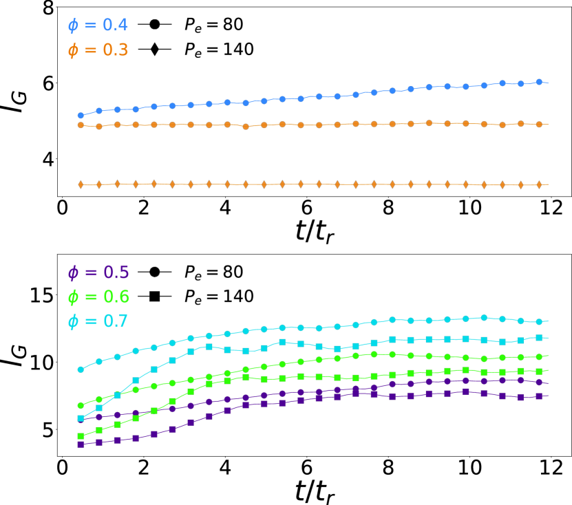
Figure 11: Average path length for systems in the frontier region (top) and in the inner region (bottom). The values for $l_{G}$ for single-phase systems(top) at $\phi=0.3$ have virtually no change over time and at $\phi=0.4$ increases slowly. In contrast, $l_{G}$ for the separated phase increases rapidly at first and then stabilizes around $t=8t_{r}$.

5 Conclusions

In this work, we have studied the dynamics of ABP using complex networks. We build a time-averaged network and concentrate on the evolution of the topology of the complex network across the MIPS region. We follow the time evolution of the degree distribution, the clustering coefficient, and the average path length, finding different structures of the complex network along the time evolution of the ABP. In the one-phase region, we developed a numerical and theoretical analysis to explain the Gaussian distribution for random graphs. Using a mean free path analysis, we found an analytical expression for the average number of unique encounters of particles in a time window $W$, showing the role of the packing fraction and Péclet number. We reported a transient region, where the degree distribution is hybrid in the sense that it is represented by two components, Gaussian and power laws, namely. Also, in the hybrid region, the average path length and average clustering coefficient do not reach a steady state at times $t=11t_{r}$.

For the two-phase region, we found that the degree distribution follows a double power law distribution with two critical exponents $\gamma_{1}\approx(1.5-3.7)$ and $\gamma_{2}\approx(12-17)$ for $k>6$. We noted that $\gamma_{1}<\gamma_{2}$, being $\gamma_{1}$ more stable over time. Moreover, we analyzed the average clustering coefficient when clustered particles are present. Because of the disk geometry, we analytically showed that this system tries to reach values around $\bar{C}=0.4$ for large packing fractions. The unexpected scaling for the average path length $l_{G}=C(\mbox{Pe})\phi^{1.2}$ is discussed, providing a simple tool to explain our results in the inner region. Our work opens exciting avenues for future research, using complex networks to characterize phase transitions in living organisms, from bacteria and ants to humans. We anticipate our study’s appeal to ecological systems, transport phenomena, multi-agent-based models, and dynamic complex networks. Furthermore, our findings introduce new possibilities for controlling and tracking clusterization in living and artificial active matter. The analytical predictions presented here can serve as a foundation for studying systems with complex interactions, including polarization, alignment, and taxis.

References

- [1] Pawel Romanczuk, Markus Bär, Werner Ebeling, Benjamin Lindner, and Lutz Schimansky-Geier. Active brownian particles: From individual to collective stochastic dynamics. The European Physical Journal Special Topics, 202:1–162, 2012.
- [2] Clemens Bechinger, Roberto Di Leonardo, Hartmut Löwen, Charles Reichhardt, Giorgio Volpe, and Giovanni Volpe. Active particles in complex and crowded environments. Reviews of Modern Physics, 88(4):045006, 2016.
- [3] Yaouen Fily and M Cristina Marchetti. Athermal phase separation of self-propelled particles with no alignment. Physical Review Letters, 108(23):235702, 2012.
- [4] Gabriel S Redner, Michael F Hagan, and Aparna Baskaran. Structure and dynamics of a phase-separating active colloidal fluid. Biophysical Journal, 104(2):640a, 2013.
- [5] Joakim Stenhammar, Davide Marenduzzo, Rosalind J Allen, and Michael E Cates. Phase behaviour of active brownian particles: the role of dimensionality. Soft Matter, 10(10):1489–1499, 2014.
- [6] Mario Theers, Elmar Westphal, Kai Qi, Roland G Winkler, and Gerhard Gompper. Clustering of microswimmers: interplay of shape and hydrodynamics. Soft Matter, 14(42):8590–8603, 2018.
- [7] Marjolein N Van Der Linden, Lachlan C Alexander, Dirk GAL Aarts, and Olivier Dauchot. Interrupted motility induced phase separation in aligning active colloids. Physical Review Letters, 123(9):098001, 2019.
- [8] Pablo de Castro, Felipe Urbina, Ariel Norambuena, and Francisca Guzmán-Lastra. Sequential epidemic-like spread between agglomerates of self-propelled agents in one dimension. Physical Review E, 108(4):044104, 2023.
- [9] Pablo de Castro, Saulo Diles, Rodrigo Soto, and Peter Sollich. Active mixtures in a narrow channel: motility diversity changes cluster sizes. Soft Matter, 17(8):2050–2061, 2021.
- [10] Gerhard Gompper, Roland G Winkler, Thomas Speck, Alexandre Solon, Cesare Nardini, Fernando Peruani, Hartmut Löwen, Ramin Golestanian, U Benjamin Kaupp, Luis Alvarez, et al. The 2020 motile active matter roadmap. Journal of Physics: Condensed Matter, 32(19):193001, 2020.
- [11] Lorenzo Caprini, Rahul Kumar Gupta, and Hartmut Löwen. Role of rotational inertia for collective phenomena in active matter. Physical Chemistry Chemical Physics, 24(40):24910–24916, 2022.
- [12] Andreas Zöttl and Holger Stark. Modeling active colloids: From active brownian particles to hydrodynamic and chemical fields. Annual Review of Condensed Matter Physics, 14:109–127, 2023.
- [13] Tzer Han Tan, Alexander Mietke, Junang Li, Yuchao Chen, Hugh Higinbotham, Peter J Foster, Shreyas Gokhale, Jörn Dunkel, and Nikta Fakhri. Odd dynamics of living chiral crystals. Nature, 607(7918):287–293, 2022.
- [14] Alexander P Petroff, Xiao-Lun Wu, and Albert Libchaber. Fast-moving bacteria self-organize into active two-dimensional crystals of rotating cells. Physical Review Letters, 114(15):158102, 2015.
- [15] Wesley JM Ridgway, Mohit P Dalwadi, Philip Pearce, and S Jonathan Chapman. Motility-induced phase separation mediated by bacterial quorum sensing. bioRxiv, pages 2023–04, 2023.
- [16] Ariel Norambuena, Felipe J Valencia, and Francisca Guzmán-Lastra. Understanding contagion dynamics through microscopic processes in active brownian particles. Scientific Reports, 10(1):20845, 2020.
- [17] P Forgács, A Libál, C Reichhardt, N Hengartner, and CJO Reichhardt. Using active matter to introduce spatial heterogeneity to the susceptible infected recovered model of epidemic spreading. Scientific Reports, 12(1):11229, 2022.
- [18] Thomas O Richardson and Thomas E Gorochowski. Beyond contact-based transmission networks: the role of spatial coincidence. Journal of The Royal Society Interface, 12(111):20150705, 2015.
- [19] Thomas E Gorochowski and Thomas O Richardson. How behaviour and the environment influence transmission in mobile groups. Temporal Network Epidemiology, pages 17–42, 2017.
- [20] Wei Zhong, Youjin Deng, and Daxing Xiong. Burstiness and information spreading in active particle systems. Soft Matter, 19(16):2962–2969, 2023.
- [21] Dhananjay Bhaskar, William Y Zhang, and Ian Y Wong. Topological data analysis of collective and individual epithelial cells using persistent homology of loops. Soft Matter, 17(17):4653–4664, 2021.
- [22] D McDermott, C Reichhardt, and CJO Reichhardt. Characterizing different motility-induced regimes in active matter with machine learning and noise. Physical Review E, 108(6):064613, 2023.
- [23] M. E. J. Newman. Scientific collaboration networks. II. Shortest paths, weighted networks, and centrality. Physical Review Journals., 64, 2001.
- [24] J. Kertész, J. Török, Y. Murase, and K. Jo, HH.and Kaski. Modeling the Complex Network of Social Interactions. In: Rudas, T., Péli, G. (eds) Pathways Between Social Science and Computational Social Science. Computational Social Sciences.Springer, Cham., https://doi.org/10.1007/978-3-030-54936-7-1, 2021.
- [25] Marta C Gonzalez, Cesar A Hidalgo, and Albert-Laszlo Barabasi. Understanding individual human mobility patterns. Nature, 453(7196):779–782, 2008.
- [26] S. Abe and N. Suzuki. Complex-network description of seismicity. Nonlinear Proc. Geophys, 13:145–150, 2006.
- [27] L. Telesca and M. Lovallo. Analysis of seismic sequences by using the method of visibility graph. . Europhysics Letters., 97, 2012.
- [28] D.Pastén, F. Torres, B. Toledo, V. Mu noz, J. Rogan, and J. A. Valdivia. Time-Based Network Analysis Before and After the M w 8.3 Illapel Earthquake 2015 Chile. Pure and Applied Geophysics., 173:2267–2275, 2016.
- [29] D. Pastén, Z. Czechowski, and B. Toledo. Time series analysis in earthquake complex networks. Chaos: An Interdisciplinary Journal of Nonlinear Science., 28, 2018.
- [30] Vinita Suyal, Awadhesh Prasad, and Harinder P Singh. Visibility-graph analysis of the solar wind velocity. Solar Physics, 289(1):379–389, 2014.
- [31] Z Mohammadi, N Alipour, H Safari, and Farhad Zamani. Complex network for solar protons and correlations with flares. Journal of Geophysical Research: Space Physics, 126(7):e2020JA028868, 2021.
- [32] J. Thiery and J. Sleeman. Complex networks orchestrate epithelial–mesenchymal transitions. Nat. Rev. Mol. Cell. Biol., 7:131–142, 2006.
- [33] A.L. Barabási, N. Gulbahce, and J. Loscalzo. Network medicine: A network-based approach to human disease. Nat. Rev. Genet., 12:56–68, 2011.
- [34] L.F.S Scabini, L.C. Ribas, M.B. Neiva, A.G.B Junior, A.J.F Farfán, and O.M. Bruno. Social interaction layers in complex networks for the dynamical epidemic modeling of covid-19 in brazil. Physica A, 564(125498):ISSN 0378–4371, 2021.
- [35] Steven Riley. Large-scale spatial-transmission models of infectious disease. Science, 316(5829):1298–1301, 2007.
- [36] Sebastian Stockmaier, Nathalie Stroeymeyt, Eric C Shattuck, Dana M Hawley, Lauren Ancel Meyers, and Daniel I Bolnick. Infectious diseases and social distancing in nature. Science, 371(6533):eabc8881, 2021.
- [37] M. E. J. Newman. The Structure and Function of Complex Networks. Society for Industrial and Applied Mathematics., 45:167–256, 2003.
- [38] Réka Albert and Albert-László Barabási. Statistical mechanics of complex networks. Rev. Mod. Phys., 74:47–97, Jan 2002.
- [39] Erdös P. and A. Rényi. On the evolution of random graphs. Publ. math. inst. hung. acad. sci, 5(1):17–60, 1960.
- [40] Albert-László Barabási and Réka Albert. Emergence of scaling in random networks. Science, 286(5439):509–512, 1999.
- [41] D. J. Watts and S. H. Strogatz. Collective dynamics of ’small-world’ networks. Nature, 393(6684):440–442, 1998.
- [42] Michael E Cates and Julien Tailleur. Motility-induced phase separation. Annu. Rev. Condens. Matter Phys., 6(1):219–244, 2015.
- [43] Ivo Buttinoni, Julian Bialké, Felix Kümmel, Hartmut Löwen, Clemens Bechinger, and Thomas Speck. Dynamical clustering and phase separation in suspensions of self-propelled colloidal particles. Physical Review Letters, 110(23):238301, 2013.
- [44] Jie Su, Mengkai Feng, Yunfei Du, Huijun Jiang, and Zhonghuai Hou. Motility-induced phase separation is reentrant. Communications Physics, 6(1):58, 2023.
- [45] M. E. J. Newman, C. Moore, and D. J. Watts. Mean-field solution of the small-world network model. Phys. Rev. Lett., 84:3201–3204, Apr 2000.
- [46] W. Li and X. Cai. Statistical analysis of airport network of china. Phys. Rev. E, 69:046106, Apr 2004.
- [47] CHI Li-Ping, WANG Ru, SU Hang, XU Xin-Ping, ZHAO Jin-Song, LI Wei, and CAI Xu. Structural properties of us flight network. Chinese Physics Letters, 20(8):1393–1396, 2003.
- [48] D. D. Han, J. H. Qian, and Y. G. Ma. Emergence of double scaling law in complex systems. Europhysics Letters, 94(2):28006, apr 2011.
- [49] Jun Zhang, Xian-Bin Cao, Wen-Bo Du, and Kai-Quan Cai. Evolution of chinese airport network. Physica A: Statistical Mechanics and its Applications, 389(18):3922–3931, 2010.
- [50] S. N. Dorogovtsev and J. F. F. Mendes. Language as an evolving word web. Proc. R. Soc. Lond. B., 268:2603–2606, 2001.
- [51] Carla M.A. Pinto, A. Mendes Lopes, and J.A. Tenreiro Machado. Double power laws, fractals and self-similarity. Applied Mathematical Modelling, 38(15):4019–4026, 2014.
Acknowledgments
The authors are grateful for the helpful feedback given Pablo de Castro. I.S and F.G.-L. have received support from the ANID – Millennium Science Initiative Program – NCN19 170, Chile. F.G.-L. was supported by Fondecyt Iniciación No. 11220683. A.N. acknowledges the financial support from the project Fondecyt Iniciación No. 11220266.