FuseMoE: Mixture-of-Experts Transformers for Fleximodal Fusion

Abstract

As machine learning models in critical fields increasingly grapple with multimodal data, they face the dual challenges of handling a wide array of modalities, often incomplete due to missing elements, and the temporal irregularity and sparsity of collected samples. Successfully leveraging this complex data, while overcoming the scarcity of high-quality training samples, is key to improving these models’ predictive performance. We introduce “FuseMoE”, a mixture-of-experts framework incorporated with an innovative gating function. Designed to integrate a diverse number of modalities, FuseMoE is effective in managing scenarios with missing modalities and irregularly sampled data trajectories. Theoretically, our unique gating function contributes to enhanced convergence rates, leading to better performance in multiple downstream tasks. The practical utility of FuseMoE in real world is validated by a challenging set of clinical risk prediction tasks.

1 Introduction

Multimodal fusion is a critical and extensively studied problem in many significant domains (Shaik et al., 2023; Yang et al., 2007; Tsai et al., 2019; Cao et al., 2023), such as sentiment analysis (Han et al., 2021b; Majumder et al., 2018), image and video captioning (Karpathy & Fei-Fei, 2015; Johnson et al., 2016b), and medical prediction (Huang et al., 2020b; Soenksen et al., 2022). Previous research has shown that embracing multimodality can improve predictive performance by capturing complementary information across modalities, outperforming single-modality approaches in similar tasks (Potamianos et al., 2003; Huang et al., 2020a). However, an ongoing challenge is the creation of scalable frameworks for fusing multimodal data, and in creating reliable models that consistently surpass their single-modal counterparts.

Table 1: We evaluated the characteristics of FuseMoE against various established benchmarks. The pipeline approach by Soenksen et al. (2022) relies on a simple feature extraction scheme for each modality, followed by concatenation and classification. The approach doesn’t incorporate irregularities or missing data in its process, but its use of concatenation and zero-imputation for missing modalities allows it to be adapted to FlexiModal settings. Both Zhang et al. (2023) and Zadeh et al. (2017) tackle multi-modality fusion issues, but as modalities increase, their method demands exponentially more cross-modal computations and significant model architecture modifications. Finally, Mustafa et al. (2022) presents MoE for language-image alignment in multimodal learning, yet it also requires substantial adjustments for the more intricate and universal FlexiModal context we explore.

Method	Type	Irregularity	Missingness	Num of Mods	Theory	Can Adapt to FlexiModal?
Soenksen et al. (2022)	Data Pipeline	✗	✗	$\geq$4	✗	✓
Zhang et al. (2023)	Modality Fusion	✓	✗	2	✗	✗
Zadeh et al. (2017)	Modality Fusion	✗	✗	3	✗	✗
Mustafa et al. (2022)	Multimodal MoE	✗	✗	2	✗	✗
FuseMoE	This Paper	✓	✓	$\geq$4	✓	Adapted

Handling a variable number of input modalities remains an open challenge in multimodal fusion, due to challenges with scalability and lack of a unified approaches for addressing missing modalities. Many existing multimodal fusion methods are designed for only two modalities (Han et al., 2021a; Zhou et al., 2019; Zhang et al., 2023), rely on costly pairwise comparisons between modalities (Tsai et al., 2019), or employ simple concatenation approaches (Soenksen et al., 2022), rendering them unable to scale to settings with a large number of input modalities or adequately capture inter-modal interactions. Similarly, existing works are either unable to handle missing modalities entirely (Zhang et al., 2023; Zhan et al., 2021) or use imputation approaches (Tran et al., 2017; Liu et al., 2023; Soenksen et al., 2022) of varying sophistication. The former methods restrict usage to cases where all modalities are completely observed, significantly diminishing their utility in settings where this is often not the case (such as in clinical applications); the latter can lead to suboptimal performance due to the inherent limitations of imputed data. In addition, the complex and irregular temporal dynamics present in multimodal data have often been overlooked (Zhang et al., 2023; Tipirneni & Reddy, 2022), with existing methods often ignoring irregularity entirely (Soenksen et al., 2022) or relying on positional embedding schemes (Tsai et al., 2019) that may not be appropriate when modalities display a varying degree of temporal irregularity. Consequently, there is a pressing need for more advanced and scalable multimodal fusion techniques that can efficiently handle a broader set of modalities, effectively manage missing and irregular data, and capture the nuanced inter-modal relationships necessary for robust and accurate prediction. We use the term FlexiModal Data to capture several of these key aspects, which haven’t been well-addressed by prior works:

“Flexi” suggests flexibility, indicating the possibility of having any combination of modalities, even with arbitrary missingness or irregularity.

A practical example of FlexiModal data can be seen in clinical applications, where extensive monitoring results in the accumulation of comprehensive electronic health records (EHRs) for each patient. A typical EHR encompasses diverse data types, including tabular data (e.g., age, demographics, gender), image data (such as X-rays, magnetic resonance imaging, and photographs), clinical notes, physiological time series (e.g., ECG and EEG) and vital signs (blood chemistry, heart rate, etc.). In this setting, we observe variety of modalities, sampled with varying irregularity and a high degree of missingness. These challenges, coupled with the relevance of predictive models to clinical settings, render ICU predictions an ideal use case to demonstrate our approach for handling FlexiModal data.

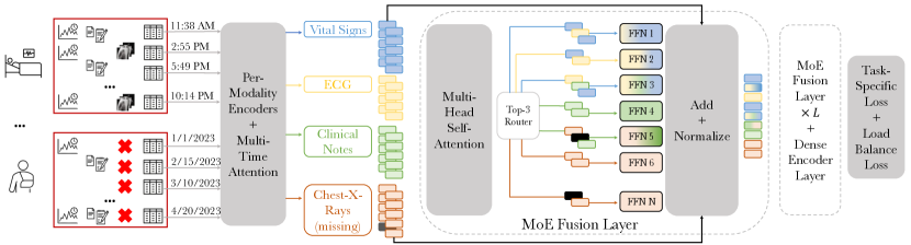
Figure 1: Addressing the challenge of FlexiModal Data in clinical scenarios: patients in ICUs often have extensive and highly irregular health status measurements over time; patients with milder conditions only require monitoring across fewer categories. FuseMoE is adept at handling EHRs featuring any combination of modalities, including those with missing elements. It starts by encoding EHRs using modality-specific feature extractors, followed by employing a multi-time attention mechanism (Shukla & Marlin, 2021) to address temporal irregularities. The core of FuseMoE lies the MoE Fusion Layer, where a routing mechanism is trained to categorize multimodal inputs and direct them to the appropriate combinations of MLPs, each tailored to process specific types of input. The outputs from these MLPs are weighted through a gating function, resulting in fused embeddings, which are subsequently utilized for further processing.

Contributions

In this paper, we introduce a novel mixture-of-experts (MoE) framework, which we call FuseMoE, specifically designed to enhance the multimodal fusion of FlexiModal Data. FuseMoE incorporates sparsely gated MoE layers in its fusion component, which are adept at managing distinct tasks and learning optimal modality partitioning. In addition, FuseMoE surpasses previous transformer-based methods in scalability, accommodating an unlimited array of input modalities. Furthermore, FuseMoE routes each modality to designated experts that specialize in those specific data types. This allows FuseMoE to adeptly handle scenarios with missing modalities by dynamically adjusting the influence of experts primarily responsible for the absent data, while still utilizing the available modalities. Lastly, another key innovation in FuseMoE is the integration of a novel Laplace gating function, which not only theoretically ensures better convergence rates compared to Softmax functions, but also demonstrates better predictive performance. We demonstrate that our approach shows superior ability, as compared to existing methods, to integrate diverse input modality types with varying missingness and irregular sampling on three challenging ICU prediction tasks.

2 Related Works

Multimodal Fusion

Initial approaches to multimodal fusion incorporated techniques such as kernel-based methods (Bucak et al., 2013; Chen et al., 2014; Poria et al., 2015), graphical models (Nefian et al., 2002; Garg et al., 2003; Reiter et al., 2007), and neural networks (Ngiam et al., 2011; Gao et al., 2015; Nojavanasghari et al., 2016). With the diverse evolution of deep learning models, numerous advanced methods have now been employed in the fusion of multimodal data. In the realm of sentiment analysis, Zadeh et al. (2017); Liu et al. (2018) employ a low-rank Tensor Fusion method that leverages both language and video content. Attention-gating mechanisms are used by Rahman et al. (2020); Yang & Wu (2021) to generate displacement vectors through cross-modal self-attention, which are then added to the input vectors from the primary modality. Tsai et al. (2019) takes an alternative approach by integrating multiple layers of cross-modal attention blocks in a word-level vision/language/audio alignment task.

In the context of clinical prediction, Khadanga et al. (2019); Deznabi et al. (2021) adopt a late fusion approach to combining vital sign and text data by concatenating embeddings from pre-trained feature extractors. Soenksen et al. (2022) developed a generalizable data preprocessing and modeling pipeline for EHR encompassing four data modalities, albeit through a direct concatenation of existing feature embeddings for each modality followed by an XGBoost classifier (Chen & Guestrin, 2016). Recently, Zhang et al. (2023) expanded on the work of Tsai et al. (2019) by introducing a discretized multi-time attention (mTAND) module (Shukla & Marlin, 2021) to encode temporal irregularities in time series and text data. Their fusion approach involves layering sets of self- and cross-modal attention blocks. However, this approach is limited to just two modalities and is not easily extendable to include additional modal components or handle missing modalities. To the best of our knowledge, existing works are tailored to application-specific settings that necessitate the computation of pairwise cross-modal relationships, which are not scalable to more general settings with arbitrary modalities. Moreover, these studies typically do not account for scenarios where modalities are missing, or rely on imputation approaches based on observed data.

Mixture-of-Experts

MoE (Jacobs et al., 1991; Xu et al., 1994) has gained significant popularity for managing complex tasks since its introduction three decades ago. Unlike traditional models that reuse the same parameters for all inputs, MoE selects distinct parameters for each specific input. This results in a sparsely activated layer, enabling a substantial scaling of model capacity without a corresponding increase in computational cost. Recent studies have demonstrated the effectiveness of integrating MoE with cutting-edge models across a diverse range of tasks (Shazeer et al., 2017; Fedus et al., 2022; Zhou et al., 2023). These works have also tackled key challenges such as accuracy and training instability (Nie et al., 2021; Zhou et al., 2022; Puigcerver et al., 2023). Given its ability to assign input partitions to specialized experts, MoE naturally lends itself to multimodal applications. This approach has been explored in fields such as vision-language modeling (Mustafa et al., 2022; Shen et al., 2023) and dynamic image fusion (Cao et al., 2023). However, the application of MoE in complex real-world settings, such as those involving FlexiModal Data, remains largely unexplored. This gap presents an opportunity to leverage MoE’s potential in handling its intricate and multifaceted nature such as multimodal EHR, where reliable multimodal integration is crucial.

MoE Theory

While MoE has been widely employed to scale up large models, its theoretical foundations have remained nascent. Recently, Nguyen et al. (2023b) provided convergence rates for both density and parameter estimation of Softmax gating Gaussian MoE. They connected these rates to the solvability of systems of polynomial equations under Voronoi-based loss functions. Later, Nguyen et al. (2024b) extended these theories to top-K sparse softmax gating MoE. Their theories further characterize the effect of the sparsity of gating functions on the behaviors of parameter estimation and verify the benefits of using top-1 sparse softmax gating MoE in practice. Other theoretical results include estimation rates of parameters and experts for multinomial logistic MoE (Nguyen et al., 2023a), for dense-to-sparse gating MoE (Nguyen et al., 2024a), and for input-independent gating MoE (Ho et al., 2022).

3 FuseMoE: Enhance Predictive Performance for FlexiModal Data

In this section, we delve into the fundamental components of FuseMoE, illustrated in Figure 1. We focus on two critical elements: the modality and irregularity encoder, and the MoE fusion layer. These components are pivotal in handling the unique characteristics of FlexiModal data.

3.1 Sparse MoE Backbone

The main components of a sparse MoE layer are a network $G$ as a sparse gate and an expert network $E$. Shazeer et al. (2017) proposed a Top-$K$ gating function that takes as an input a token representation $x\in\mathbb{R}^{D}$ and then routes it to the Top-$K$ experts out of the set $\{E_{i}\}_{i=1}^{S}$. The gating network variable $W\in\mathbb{R}^{D\times N}$ produces logits $h_{s}(x)=\mathrm{Top~{}K}(W\cdot x)$, which are normalized via Softmax:

$$G(x)_{i}=\frac{\exp(h_{s}(x)_{i})}{\sum_{j}^{K}\exp(h_{s}(x)_{j})}$$ (1)

Each expert network ($E_{i}:\mathbb{R}^{D}\rightarrow\mathbb{R}^{D}$) contains a feed-forward layer (FFN) and its parameters are independent of other models. The final output of the expert network $y$ is the linearly weighted combination of each expert’s output on the token by the gate’s output: $y=\sum_{i=1}^{S}G(x)_{i}E_{i}(x)$.

Gating Function Softmax gating, commonly used as a gating function in various tasks, is contrasted with Gaussian gated MoE, a popular alternative noted for its distinct advantages. Initially introduced by Xu et al. (1994), Gaussian gating is recognized for its superior qualities in certain scenarios, as compared to Softmax gating. The nonlinearity of the Softmax function complicates the application of the expectation-maximization (EM) algorithm. In contrast, Gaussian gating overcomes this difficulty with an analytical solution during the $M$-step. Additionally, it offers enhanced localization properties, crucial for minimizing interference among experts, a benefit that becomes increasingly significant as the number of experts in the model grows (Ramamurti & Ghosh, 1998). The logits of the Gaussian gating function are formulated as follows:

$$h_{g}(x)=\mathrm{Top~{}K}(-\|W-x\|_{2}^{2}).$$ (2)

The incorporation of Gaussian gating facilitates the convergence of the EM algorithm. Building upon this, our paper introduces an innovative Laplace gating function. This new function’s logit is formulated as follows:

$$h_{l}(x)=\mathrm{Top~{}K}(-\|W-x\|_{2}).$$ (3)

The Laplace gating function, characterized by its Euclidean term $\exp(-\|W-x\|_{2})$, is less prone to converge towards extreme weight distributions due to the bounded nature of this term. In subsequent sections, we will illustrate how this gating function facilitates faster parameter estimation rates compared to Gaussian and Softmax gating. Moreover, our empirical findings indicate that the Laplace gating exhibits enhanced performance in managing multimodal data.

3.2 Modality and Irregularity Encoder

To encode the irregularity of sampling in each modality, we utilize a discretized multi-time attention (mTAND) module (Shukla & Marlin, 2021), which leverages a time attention mechanism (Kazemi et al., 2019; Vaswani et al., 2017) to discretize irregularly sampled observations into discrete intervals. Specifically, given a set of $l_{k}$ continuous time points, $t\in\mathbb{R}^{l_{k}}$, corresponding to the $k^{\mathrm{th}}$ dimensionality of a given modality, we employ $H$ embedding functions $\phi_{h}(\tau)$ to embed each $\tau_{k}\in t_{k}$ in a $d_{h}$ dimensional space. The $i^{\mathrm{th}}$ dimension of the $h^{\mathrm{th}}$ embedding is defined as

$$\phi_{h}(\tau)[i]=\begin{cases}w_{i}\tau_{k},&\text{if }i=1\\ \sin(w_{i}\tau_{k}+\phi_{i}),&\text{if }1<i\leq d_{h},\end{cases}$$

where $\{w_{i},\phi_{i}\}_{i=1}^{d_{h}}$ are learnable parameters. By performing this for each continuous time point in $t_{k}$, we create a $d_{h}$ dimensional representation of each time point in $H$ different embedding spaces. We then leverage these embeddings to discretize the irregularly sampled observations into discretized bins. Specifically, we seek to discretize $x_{k}$ (with $l_{k}$ corresponding observation times $t_{k}$) into $\gamma$ regularly sampled intervals $\bm{\gamma}$. We do this via an attention mechanism, which, for each embedding function $\phi_{h}(\tau)$, takes $\bm{\gamma}$ as queries, $t_{k}$ as keys, and $x_{k}$ as values and produces $\hat{x}_{k,h}\in\mathbb{R}^{\gamma}$ embeddings for each sequence. Formally,

$$\hat{x}_{k,h}=\text{softmax}\left(\frac{\phi_{h}(\bm{\gamma})\mathbf{Q}_{h}\mathbf{K}_{h}^{\top}\phi_{h}(t_{k})^{\top}}{\sqrt{l_{k}}}\right)x_{k},$$

where $\mathbf{Q}_{h}$ and $\mathbf{K}_{h}$ are learnable parameters. This formulation allows us to discretize univariate observations $x_{k}$ into $\gamma$ regularly-sampled bins. To model irregularity across a multivariate set of observations for a given modality with $d_{m}$ dimensions, we repeat this process for each dimension of the input. This allows us to obtain an interpolation matrix $\hat{X}_{h}=[\hat{x}_{1,h},\hat{x}_{2,h},...,\hat{x}_{d_{m},h}]\in\mathbb{R}^{\gamma\times d_{m}}$ for each of the $h$ embedding functions. We then concatenate the interpolation matrices across all $H$ embedding functions (i.e., $I=[\hat{X}_{1},\hat{X}_{2},...,\hat{X}_{h}]\in\mathbb{R}^{\gamma\times(H\cdot d_{m})}$) and employ a linear projection to achieve a final, discretized embedding for each modality, $Z\in\mathbb{R}^{\gamma\times d_{e}}$, where $d_{e}$ denotes the desired dimensionality of each modality’s representation. Appendix C discusses further details of the embedding.

Figure 2: We present three exemplary designs of the Tok-$K$ router for effective multimodal fusion, considering an input scenario with three modalities: Time-Series (TS), Text (TXT), and Chest X-Rays (CXR). (a) The joint router design utilizes a concatenated embedding of all modalities, directing this combined input to selected experts. (b) In the modality-specific router design, each modality’s embedding is independently assigned to a shared pool of experts. (c) The third design variant also uses modality-specific routers but assigns each modality’s embedding to separate pools of experts, each pool uniquely tailored to process a specific modality type.

Encoding Multiple Modalities The process described above allows us to discretize an arbitrarily long irregular, multivariate sequence into a regularly sampled, discretized embedding with length $\gamma$ and dimensionality $d_{e}$. We repeat this for each of the $M$ modalities, to create $M$ embeddings, $\{Z_{j}\}_{j=1}^{M}$, which are then combined to generate predictions.

3.3 MoE Fusion Layer

Router Design Study

Upon obtaining embeddings from each of the $j$ modalities, we propose multiple complementary approaches for processing multimodal inputs. Figure 2 illustrates a range of router design options. The most straightforward strategy involves employing a common router that handles the concatenated embeddings of all $j$ modalities, without imposing any gating constraints. As the complexity increases with additional modalities, we consider more sophisticated alternatives: deploying separate routers for each modality’s embedding and assigning these embeddings to a shared pool of experts. This allows for distinct processing while maintaining a unified expert framework. Additionally, we further segregate these common expert pools, allowing each router to direct its respective embedding to dedicated experts skilled in handling such specific inputs. These varied router design choices offer users enhanced flexibility, enabling more fine-grained control of both inter-modal and intra-modal relationships.

We implement an entropy regularization loss to ensure balanced and stable expert utilization, a concept supported by various previous studies (Mustafa et al., 2022; Meister et al., 2020; Genevay, 2019). It maximizes the mutual information between modalities and experts and serves as an auxiliary loss function in addition to task-specific loss. Given a total of $M$ modalities, and denoting $\mathcal{H}$ as the entropy, we define the loss function $\mathcal{E}$ as follows:

$$\mathcal{E}(x)=\frac{1}{M}\sum_{j=1}^{M}\mathcal{H}(\hat{p}_{m_{j}}(E))-\mathcal{H}(\frac{1}{M}\sum_{j=1}^{M}\hat{p}_{m_{j}}(E)),$$ (4)

where $\hat{p}_{m_{j}}(E)$ is the probability distribution over the experts $\{E_{i}\}_{i=1}^{S}$ for the $j^{\mathrm{th}}$ modality. This distribution can be approximated by $\hat{p}_{m_{j}}(E)=\frac{1}{l^{j}}\sum_{i=1}^{l^{j}}p_{m_{j}}(E~{}|~{}x_{i}^{m_{j}})$, where $l^{j}$ is the number of observations of the $j^{\mathrm{th}}$ modality. Intuitively, we actively encourage the input embeddings to diminish the uncertainty in selecting experts. By incorporating the loss $\mathcal{E}$, we aim to stabilize the experts’ preferences within each modality, while concurrently promoting a diverse range of expert selections across modalities.

Missing Modalities

In scenarios where certain modalities are missing throughout the data trajectories, we substitute the original embedding $Z_{\mathrm{missing}}$ with a learnable embedding $\mathcal{Z}$, acting as a “missing indicator”. This strategy is facilitated by employing per-modality routers, which, in conjunction with entropy regularization, guide $\mathcal{Z}$ predominantly toward a specific group of less-utilized experts. The new embeddings $\mathcal{Z}$ are dynamically adjusted throughout the model training process to simultaneously minimize the task-specific loss and the entropy regularization loss. As a result, the router will assign lower weights to the experts responsible for processing these embeddings.

4 Theoretical Justification

In this section, we provide a theoretical guarantee of the benefits of the Laplace gating function over the standard softmax gating function in MoE. In particular, we conduct a convergence analysis for maximum likelihood estimation (MLE) under the Laplace gating Gaussian MoE and prove that the MLE in Laplace gating MoE has better convergence behaviors than that in softmax gating MoE.

Notations We denote $[n]:=\{1,2,\ldots,n\}$ for any $n\in\mathbb{N}$. Additionally, the notation $|S|$ indicates the cardinality of a given set $S$. For any vector $v\in\mathbb{R}^{d}$, $\|v\|$ stands for its $2$-norm value. Finally, for any two probability densities $p,q$ dominated by the Lebesgue measure $\mu$, we denote $V(p,q)=\frac{1}{2}\int|p-q|d\mu$ as their Total Variation distance.

Table 2: Summary of parameter estimation rates under the softmax and Laplace gating Gaussian MoE models. In this table, the function $\widetilde{r}(\cdot)$ represents for the solvability of a system of polynomial equations considered in (Nguyen et al., 2023b) with a note that $\widetilde{r}(\cdot)\leq\bar{r}(\cdot)$ and $\widetilde{r}(2)=4$, $\widetilde{r}(3)=6$. Additionally, $\mathcal{A}^{n}_{j}:=\mathcal{A}_{j}(\widehat{G}_{n})$ denotes a Voronoi cell defined in equation 7.

Gates	$\exp(\beta_{j}^{*})$	$W_{j}^{*}$	$a_{j}^{*}$	$b^{*}_{j}$	$\nu_{j}^{*}$
Softmax (Nguyen et al., 2023b)	$\mathcal{O}(n^{-1/2})$	$\mathcal{O}(n^{-1/2\widetilde{r}(|\mathcal{A}^{n}_{j}|)})$	$\mathcal{O}(n^{-1/\widetilde{r}(|\mathcal{A}^{n}_{j}|)})$	$\mathcal{O}(n^{-1/2\widetilde{r}(|\mathcal{A}^{n}_{j}|)})$	$\mathcal{O}(n^{-1/\widetilde{r}(|\mathcal{A}^{n}_{j}|)})$
Laplace (Ours)	$\mathcal{O}(n^{-1/2})$	$\mathcal{O}(n^{-1/4})$	$\mathcal{O}(n^{-1/4})$	$\mathcal{O}(n^{-1/2\bar{r}(|\mathcal{A}^{n}_{j}|)})$	$\mathcal{O}(n^{-1/\bar{r}(|\mathcal{A}^{n}_{j}|)})$

Problem Setup Assume that $(X_{1},Y_{1}),\ldots,(X_{n},Y_{n})\in\mathbb{R}^{d}\times\mathbb{R}$ are i.i.d. samples drawn from the Laplace gating Gaussian MoE of order $k_{*}$ whose conditional density function $p_{G_{*}}(Y|X)$ is given by:

$$p_{G_{*}}(Y|X)=\sum_{i=1}^{k_{*}} \mathrm{softmax}(\mathrm{TopK}(-\|W_{i}^{*}-X\|,K;\beta_{i}^{*}))$$

$$\hskip 20.00003pt\times f(Y|(a_{i}^{*})^{\top}X+b_{i}^{*},\nu_{i}^{*}),$$ (5)

where $f(\cdot|\mu,\sigma)$ denotes a univariate Gaussian density function with mean $\mu$ and variance $\sigma$. For the simplicity of the presentation, we denote $G_{*}:=\sum_{i=1}^{k_{*}}\exp(\beta_{i}^{*})\delta_{(W_{i}^{*},a_{i}^{*},b_{i}^{*},\nu_{i}^{*})}$ as a true but unknown mixing measure associated with true parameters $(\beta_{i}^{*},W_{i}^{*},a_{i}^{*},b_{i}^{*},\nu_{i}^{*})$ for $i\in\{1,2,\ldots,k_{*}\}$. Here, $\delta$ denotes the Dirac delta measure. In the paper, we specifically consider two settings of the true number of experts $k_{*}$: (i) Exact-specified setting: when $k_{*}$ is known; (ii) Over-specified setting: when $k_{*}$ is unknown, and we over-specify the model in equation 4 by a Laplace gating MoE model with $k>k_{*}$ experts. However, due to the space limit, we present only the latter setting, and defer the former setting to Appendix G.

Maximum Likelihood Estimation We use the maximum likelihood method to estimate the unknown mixing measure $G_{*}$. Notably, under the over-specified setting, as the true density $p_{G_{*}}(Y|X)$ is associated with top $K$ experts which are possibly approximated by more than $K$ fitted experts, we need to select $\overline{K}>K$ experts in the formulation of density estimation to guarantee its convergence to $p_{G_{*}}(Y|X)$. In particular, the MLE is given by

$$\widehat{G}_{n}\in\operatorname*{arg\,max}_{G\in\mathcal{G}_{k}(\Theta)}\frac{1}{n}\sum_{i=1}^{n}\log(\overline{p}_{G}(Y_{i}|X_{i})),$$ (6)

where $\mathcal{G}_{k}(\Theta):=\{G=\sum_{i=1}^{k}\exp(\beta_{i})\delta_{(W_{i},a_{i},b_{i},\nu_{i})}:(W_{i},a_{i},b_{i},\nu_{i})\in\Theta\}$ denotes the set of all mixing measures with at most $k$ components and

$$\overline{p}_{G}(Y|X)=\sum_{i=1}^{k_{*}}\mathrm{softmax}( \mathrm{TopK}(-\|W_{i}-X\|,\overline{K};\beta_{0i}))$$

$$\times f(Y|(a_{i})^{\top}X+b_{i},\nu_{i}).$$

Given the MLE defined in equation 6, we first demonstrate that the conditional density function $p_{\widehat{G}_{n}}$ also converges to its true counterpart $p_{G_{*}}$ at the parametric rate.

Theorem 4.1.

The density estimation $\overline{p}_{\widehat{G}_{n}}(Y|X)$ converges to the true density $p_{G_{*}}(Y|X)$ under the Total Variation distance $V$ at the following rate:

$$\mathbb{E}_{X}[V(\overline{p}_{\widehat{G}_{n}}(\cdot|X),p_{G_{*}}(\cdot|X))]=\mathcal{O}(\sqrt{\log(n)/n}).$$

Proof of Theorem 4.1 is in Appendix H.3. The parametric rate of the conditional density function $p_{\widehat{G}_{n}}$ indicates that we only need to determine a loss function between the MLE and the true mixing measure to lower bound the total variation distance between $p_{\widehat{G}_{n}}$ and $p_{G_{*}}$.

Table 3: Comparison of FuseMoE-based methods (gray) and baselines, utilizing vital signs and clinical notes of MIMIC-IV. The best results are highlighted in bold font, and the second-best results are underlined. All results are averaged across 3 random experiments.

Task $\backslash$ Method				MISTS	MulT	MAG	TF	HAIM	Softmax	Gaussian	Laplace
48-IHM	AUROC	75.06 $\pm$ 1.03	75.95 $\pm$ 0.84	75.82 $\pm$ 0.73	78.76 $\pm$ 0.79	79.65 $\pm$ 0.00	79.49 $\pm$ 0.83	80.76 $\pm$ 0.56	81.03 $\pm$ 0.25
	F1	45.61 $\pm$ 0.34	38.81 $\pm$ 0.22	42.55 $\pm$ 0.82	40.61 $\pm$ 0.41	39.79 $\pm$ 0.00	42.86 $\pm$ 0.44	46.86 $\pm$ 0.24	46.53 $\pm$ 0.57
LOS	AUROC	80.56 $\pm$ 0.33	81.36 $\pm$ 1.32	81.13 $\pm$ 0.66	80.71 $\pm$ 0.45	82.58 $\pm$ 0.00	82.11 $\pm$ 0.39	81.92 $\pm$ 0.73	82.91 $\pm$ 1.02
	F1	73.01 $\pm$ 0.52	73.45 $\pm$ 0.59	72.51 $\pm$ 0.27	73.84 $\pm$ 0.61	73.18 $\pm$ 0.00	74.43 $\pm$ 0.88	74.46 $\pm$ 0.52	74.58 $\pm$ 0.63
25-PHE	AUROC	69.45 $\pm$ 0.72	66.58 $\pm$ 0.41	69.55 $\pm$ 0.67	69.18 $\pm$ 0.32	63.39 $\pm$ 0.00	70.54 $\pm$ 0.47	70.42 $\pm$ 0.26	71.23 $\pm$ 0.53
	F1	28.59 $\pm$ 0.46	28.55 $\pm$ 0.31	27.86 $\pm$ 0.29	28.52 $\pm$ 0.22	42.13 $\pm$ 0.00	31.25 $\pm$ 0.18	30.44 $\pm$ 0.27	31.33 $\pm$ 0.19

Table 4: Incorporating CXR and ECG into FuseMoE leads to a noticeable enhancement as compared to their two-modality counterparts.

Task $\backslash$ Method				Vital & Notes & CXR				Vital & Notes & CXR & ECG
		HAIM	Softmax	Gaussian	Laplace	HAIM	Softmax	Gaussian	Laplace
48-IHM	AUROC	78.87 $\pm$ 0.00	83.13 $\pm$ 0.36	83.64 $\pm$ 0.47	83.87 $\pm$ 0.33	78.87 $\pm$ 0.00	82.92 $\pm$ 0.22	83.03 $\pm$ 0.85	83.55 $\pm$ 0.49
	F1	39.78 $\pm$ 0.00	46.82 $\pm$ 0.28	38.87 $\pm$ 0.26	45.36 $\pm$ 0.46	39.78 $\pm$ 0.00	46.87 $\pm$ 0.17	44.04 $\pm$ 0.26	46.88 $\pm$ 0.42
LOS	AUROC	82.46 $\pm$ 0.00	83.76 $\pm$ 0.59	83.64 $\pm$ 0.52	83.51 $\pm$ 0.51	82.46 $\pm$ 0.00	83.53 $\pm$ 0.34	83.47 $\pm$ 0.37	83.58 $\pm$ 0.78
	F1	72.75 $\pm$ 0.00	74.32 $\pm$ 0.44	76.59 $\pm$ 0.74	75.18 $\pm$ 0.77	72.75 $\pm$ 0.00	75.01 $\pm$ 0.63	74.43 $\pm$ 0.64	75.11 $\pm$ 0.65
25-PHE	AUROC	63.57 $\pm$ 0.00	73.87 $\pm$ 0.71	72.68 $\pm$ 0.61	73.65 $\pm$ 0.39	63.82 $\pm$ 0.00	73.64 $\pm$ 0.89	73.74 $\pm$ 0.41	73.67 $\pm$ 0.71
	F1	42.80 $\pm$ 0.00	35.96 $\pm$ 0.23	35.09 $\pm$ 0.15	36.01 $\pm$ 0.42	43.20 $\pm$ 0.00	36.06 $\pm$ 0.17	36.46 $\pm$ 0.55	35.81 $\pm$ 0.34

Voronoi Loss We now define a loss function between the MLE and the true mixing measure. Given some mixing measure $G:=\sum_{i=1}^{k}\exp(\beta_{i})\delta_{(W_{i},a_{i},b_{i},\nu_{i})}$, we distribute its components to the following Voronoi cells $\mathcal{A}_{j}\equiv\mathcal{A}_{j}(G)$ which are generated by the support of the true mixing measure $G_{*}:=\sum_{j=1}^{k_{*}}\exp(\beta_{j}^{*})\delta_{(W_{j}^{*},a_{j}^{*},b_{j}^{*},\nu_{j}^{*})}$:

$$\mathcal{A}_{j}:=\{i\in[k]:\|\theta_{i}-\theta^{*}_{j}\|\leq\|\theta_{i}-\theta^{*}_{\ell}\|,\ \forall\ell\neq j\},$$ (7)

where $\theta_{i}:=(W_{i},a_{i},b_{i},\nu_{i})$ and $\theta^{*}_{j}:=(W_{j}^{*},a_{j}^{*},b_{j}^{*},\nu_{j}^{*})$ for any $1\leq i\leq k$ and $1\leq j\leq k_{*}$. Based on these Voronoi cells, we propose the following Voronoi loss function for the over-specified setting:

$$\mathcal{D}_{2}(G,G_{*}):=\max\Bigg{[}\Big{|}\sum_{i\in\mathcal{A}_{\tau_{j}}}\exp(\beta_{i})-\exp(\beta^{*}_{\tau_{j}})\Big{|}$$

$$+\sum_{j\in[K]:|\mathcal{A}_{\tau_{j}}|>1}\sum_{i\in\mathcal{A}_{\tau_{j}}}\exp(\beta_{i})\Phi_{i\tau_{j}}\Big{(}2,2,\bar{r}(|\mathcal{A}_{\tau_{j}}|),\frac{\bar{r}(|\mathcal{A}_{\tau_{j}}|)}{2}\Big{)}$$

$$+\sum_{j\in[K]:|\mathcal{A}_{\tau_{j}}|=1}\sum_{i\in\mathcal{A}_{\tau_{j}}}\exp(\beta_{i})\Phi_{i\tau_{j}}(1,1,1,1)\Bigg{]},$$ (8)

where the maximum in the definition of Voronoi loss function $\mathcal{D}_{2}$ is for $\{\tau_{1},\tau_{2},\ldots,\tau_{K}\}\subseteq[k_{*}]$. Furthermore, for any $(\rho_{1},\rho_{2},\rho_{3},\rho_{4})\in\mathbb{R}^{4}$, we define $\Phi_{i\tau_{j}}(\rho_{1},\rho_{2},\rho_{3},\rho_{4})=\|W_{i}-W_{\tau_{j}}^{*}\|^{\rho_{1}}+\|a_{i}-a_{\tau_{j}}^{*}\|^{\rho_{2}}+|b_{i}-b_{\tau_{j}}^{*}|^{\rho_{3}}+|\nu_{i}-\nu_{\tau_{j}}^{*}|^{\rho_{4}}$ for any $i\in\mathcal{A}_{\tau_{j}}$ and $j\in[K]$. Additionally, the notation $\bar{r}(|\mathcal{A}_{\tau_{j}}|)$ stands for the minimum value of $r\in\mathbb{N}$ such that the following system of polynomial equations:

$$\sum_{i=1}^{|\mathcal{A}_{\tau_{j}}|}\sum_{\begin{subarray}{c}m_{1}+2m_{2}=s,\\ 1\leq m_{1}+m_{2}\leq r\end{subarray}}\frac{q_{3i}^{2}q_{1i}^{m_{1}}q_{2i}^{m_{2}}}{m_{1}!m_{2}!}=0,~{}\text{for each }s=1,2,\ldots,r,$$ (9)

does not have any non-trivial solutions for the unknown variables $\{(q_{1i},q_{2i},q_{3i})\}_{i=1}^{|\mathcal{A}_{\tau_{j}}|}$. A solution to the above system is regarded as non-trivial if at least among variables $q_{1i}$ is different from zero, whereas all the variables $q_{3i}$ are non-zero. It is worth noting that the function $\bar{r}(\cdot)$ was previously studied in Ho & Nguyen (2016) to characterize the convergence behavior of parameter estimation under the location-scale Gaussian mixture models. Ho & Nguyen (2016) also gave some specific values of that function, namely $\bar{r}(2)=4$ and $\bar{r}(3)=6$. Meanwhile, they claimed that it was non-trivial to determine the value of $\bar{r}(m)$ when $m\geq 4$, and further techniques should be developed for that purpose. Since Gaussian MoE models are generalization of the Gaussian mixture models, we also involve the function $\bar{r}(\cdot)$ in our convergence analysis.

Theorem 4.2.

When $k>k_{*}$ becomes unknown, the following Total Variation bound holds true for any $G\in\mathcal{G}_{k}(\Theta)$:

$$\mathbb{E}_{X}[V(\overline{p}_{G}(\cdot|X),p_{G_{*}}(\cdot|X))]\gtrsim\mathcal{D}_{2}(G,G_{*}).$$

Consequently, we obtain $\mathcal{D}_{2}(\widehat{G}_{n},G_{*})=\mathcal{O}(\sqrt{\log(n)/n})$.

Proof of Theorem 4.2 is in Appendix H.4. The results of Theorem 4.2 together with the formulation of the loss function $\mathcal{D}_{2}$ in equation 4 reveal that (see also Table 2):

(i) Parameters $W^{*}_{i},a^{*}_{i},b^{*}_{i},\nu^{*}_{i}$ which are fitted by exactly one component, i.e. $|\mathcal{A}^{n}_{i}|:=|\mathcal{A}_{i}(\widehat{G}_{n})|=1$, enjoy the same estimation rate of order $\mathcal{O}(n^{-1/2})$ (up to some logarithmic factor), which match those in Nguyen et al. (2023b).

(ii) The rates for estimating parameters $W^{*}_{i},a^{*}_{i},b^{*}_{i},\nu^{*}_{i}$ which are fitted by more than one component, i.e. $|\mathcal{A}^{n}_{i}|>1$, are no longer homogeneous. On the one hand, the estimation rates for parameters $b^{*}_{i}$ and $\nu^{*}_{i}$ are of orders $\mathcal{O}(n^{-1/2\bar{r}(|\mathcal{A}^{n}_{i}|)})$ and $\mathcal{O}(n^{-1/\bar{r}(|\mathcal{A}^{n}_{i}|)})$, respectively, both of which are determined by the function $\bar{r}(\cdot)$ and vary with the number of fitted components $|\mathcal{A}^{n}_{i}|$. Those rates are comparable to their counterparts in Nguyen et al. (2023b). On the other hand, gating parameters $W^{*}_{i}$ and expert parameters $a^{*}_{i}$ share the same estimation rate of order $\mathcal{O}(n^{-1/4})$, which remains constant with respect to the number of fitted components. Meanwhile, those rates in Nguyen et al. (2023b) depend on the solvability of a different system of polynomial equations from that in equation 9, which are significantly slower.

5 Experiments

In this section, we demonstrate empirically that FuseMoE is capable of providing accurate and efficient predictions when applied to FlexiModal datasets. The broad applicability of FlexiModal data means that real-world applications are plentiful. We note that ICU data are particularly rich in this context, featuring a diverse range of measurements across multiple modalities, motivating our focus on three tasks highly relevant to critical care settings (Keuning et al., 2020). The urgency of care in the ICU necessitates swift and accurate assessments of patient conditions to guide decisions, but current methods fail to incorporate information beyond acute physiology (Awad et al., 2017a).

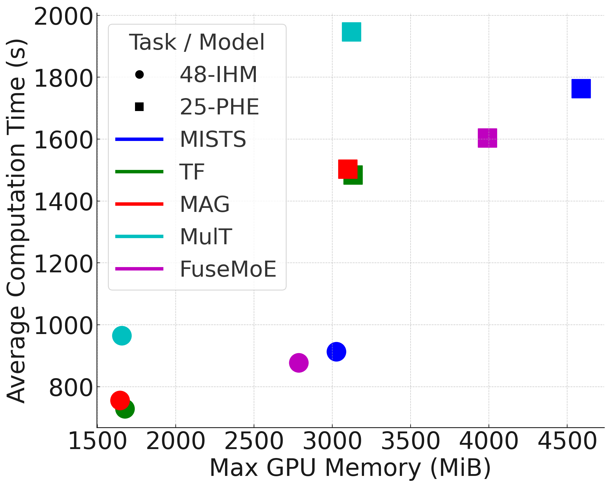
(a)

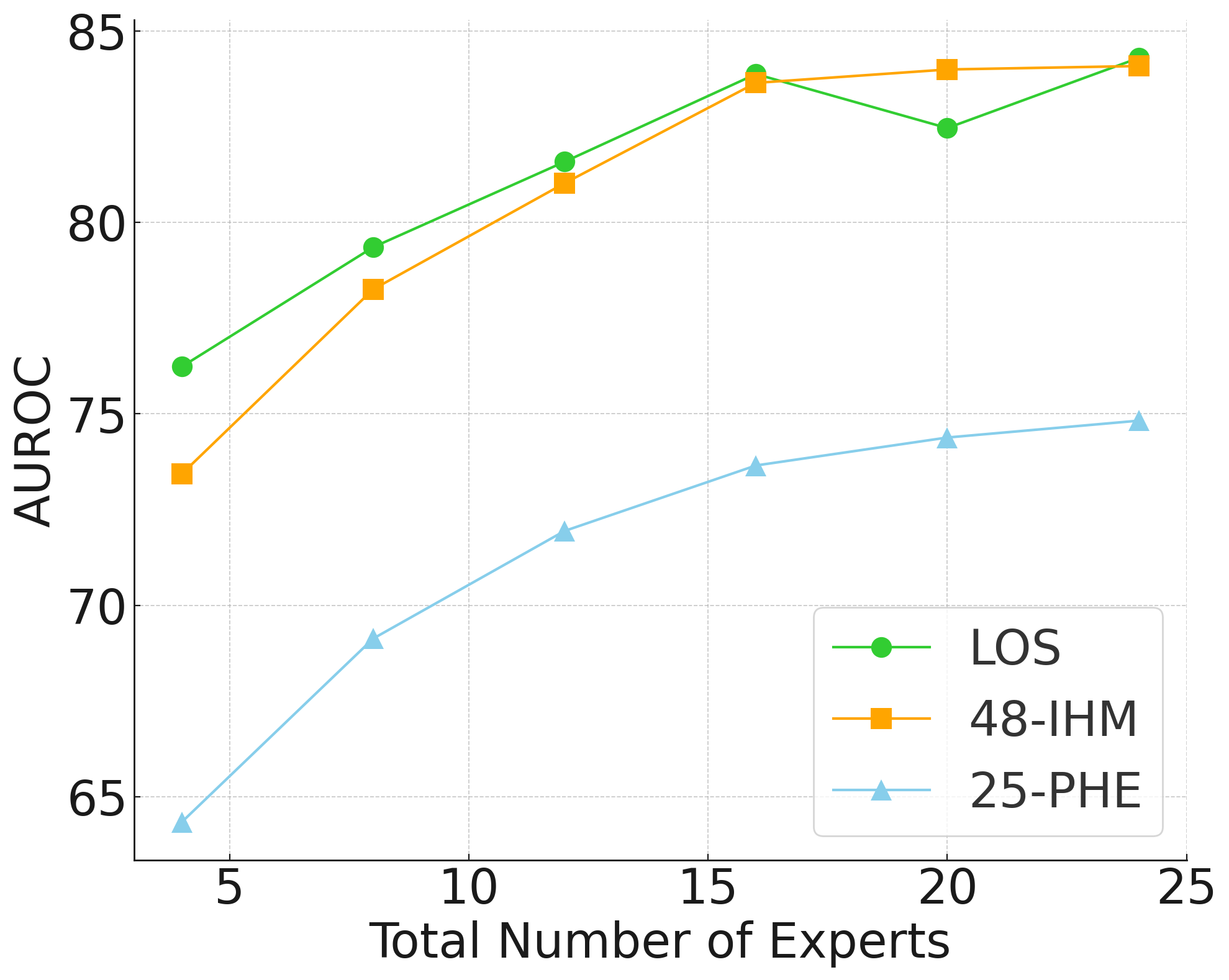
(b)

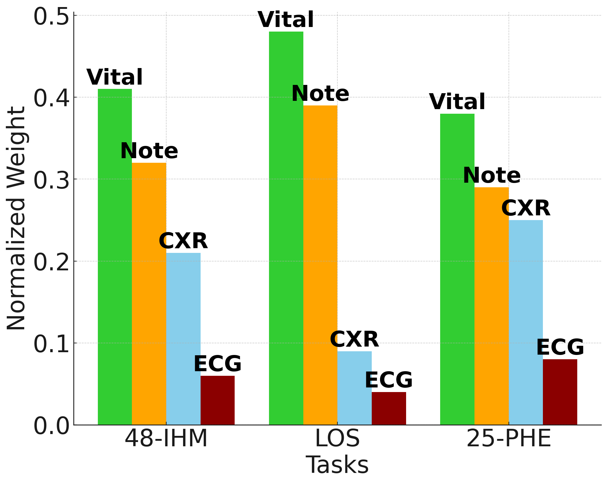
(c)

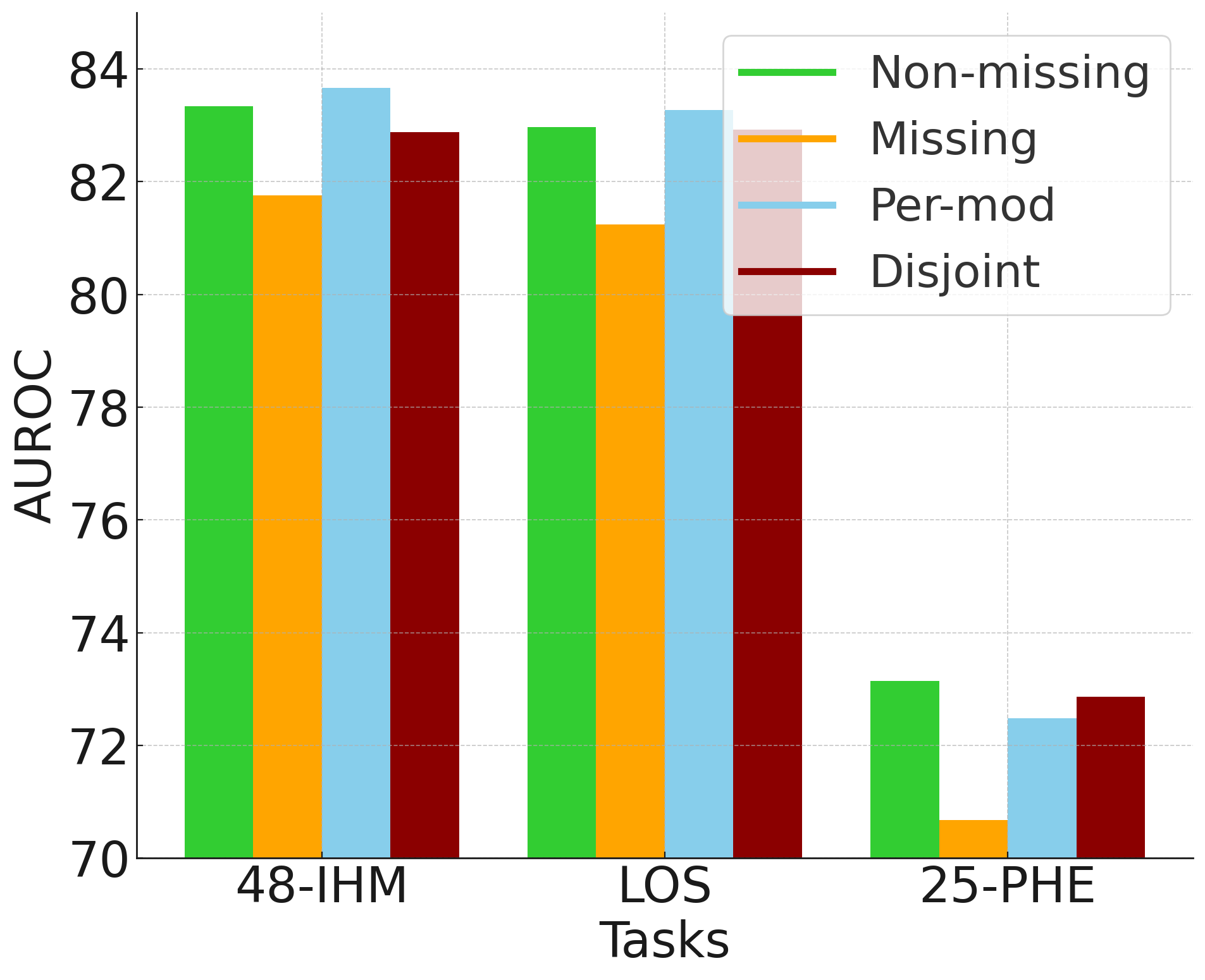
(d)

Figure 3: Results of ablation studies: (a) The computational efficiency and resource utilization of each method when applied to vital signs and clinical notes from the MIMIC-IV dataset; (b) The relationship between the number of experts and task performance across different modalities, including vital signs, clinical notes, and CXR; (c) The impact of each modality on the top-$k$ experts within a disjoint router structure; (d) The role of per-modality routers and the entropy loss $\mathcal{E}$ in mitigating the impact of missing modalities.

Experimental Setup

We leveraged data from MIMIC-IV (Johnson et al., 2020) and its predecessor, MIMIC-III (Johnson et al., 2016a). Our tasks of interest include the 48-hour in-hospital mortality prediction (48-IHM), 25-type phenotype classification (25-PHE), and length-of-stay (LOS) prediction. The baselines include HAIM (Soenksen et al., 2022), multimodal fusion via cross-attention (MulT) (Tsai et al., 2019), cross-attention combined with irregular sequences (MISTS) (Zhang et al., 2023), tensor fusion (TF) (Zadeh et al., 2017), and multimodal adaptation gate (MAG) (Rahman et al., 2020). All details of the experimental setup can be found in Appendices A - E.

5.1 Primary Results

Table 3 shows the outcomes of combining irregular vital signs and clinical notes from the MIMIC-IV dataset. The FuseMoE-based methods surpass baselines in most scenarios, often by a non-trivial margin. The Laplace gating function also outperforms its counterparts, aligning with our theoretical claims. Furthermore, we observe that HAIM shows considerable efficacy in extracting features from time series, resulting in a strong performance in the 48-IHM and LOS tasks, which are heavily reliant on such data. However, its performance appears more moderate on the 25-PHE task. Note that, the results derive from the MIMIC-IV dataset without missing modalities. We used the “joint experts and router” configuration, given that alterations to the router design did not significantly impact performance in this context. Overall, the results have shown the efficacy of integrating the irregularity encoder with the MoE fusion layer. Additional results on (1) the MIMIC-III data and (2) combining vital signs with CXR can be found in Appendix F.

Additional Modalities

We then expand the FuseMoE framework to incorporate additional modalities. Note that, except for HAIM, the baselines were not designed to be agnostic to the quantity and variety of input modalities. Therefore, adapting them to manage extra and missing modalities requires considerable model changes, which might compromise their performance. Table 4 presents the revised outcomes after integrating extra modalities, employing the per-modality router and the entropy loss $\mathcal{E}$ within FuseMoE. This setup was chosen as it slightly outperformed the joint router with an increase in modalities. Relative to their two-modality versions, FuseMoE has effectively harnessed additional information (notably from CXR), resulting in a significant enhancement in performance. Conversely, the addition of new modalities did not benefit the HAIM method, possibly due to its reliance on vital signs and clinical notes without adequately addressing the dynamics between different modalities. Furthermore, HAIM’s notably high F1 scores on the 25-PHE task can be attributed to XGBoost’s proficiency in managing missing minority classes.

5.2 Ablation Studies

We then conducted ablation studies to explore the various attributes of FuseMoE and baselines. Figure 3(a) examines the computational efficiency and resource utilization, positioning FuseMoE approximately in the middle of the comparison. Despite the increase in model parameters due to the incorporation of the MoE layer, its sparse nature does not significantly escalate the computational load. Figure 3(b) illustrates the correlation between the number of experts and task performance across different modalities. Generally, performance improves with the addition of more experts, plateauing once the count exceeds 16. To achieve a compromise between performance and computational expense, we opted to utilize the top 4 experts out of 16 in our experiments. Figure 3(c) studies the influence of each modality on the top-$k$ chosen experts. For every expert selected, we calculate the number of samples that include a specific modality, weighted by corresponding weight factors from the gating functions. The outcomes are subsequently normalized across modalities. The analysis reveals that predictions across all tasks heavily depend on vital signs and clinical notes. This reliance is attributed to the abundant samples in these two modalities. Despite the notably smaller quantity of CXR, they play more significant roles in the 25-PHE and 48-IHM tasks, which aligns with our findings in Table 4. Lastly, Figure 3(d) illustrates the effectiveness of utilizing per-modality routers and the entropy loss $\mathcal{E}$ in addressing missing modalities. Initially, we compare the performance of FuseMoE on patients with fully available modalities against those with missing components, employing a joint router mechanism with the importance loss function (Shazeer et al., 2017), to ensure load balancing. The inclusion of datasets with missing modalities, while expanding the sample size, resulted in a decrease in overall performance due to the compromised data quality. However, an enhancement in performance was observed upon integrating per-modality or disjoint routers with $\mathcal{E}$. Notably, the outcomes for the 48-IHM and LOS tasks with missing modalities surpassed those obtained from datasets without any missing data. This is because the per-modality structure can better separate the present and missing modalities, reducing the influence of experts responsible for processing the absent inputs. Therefore, this leads to a more efficient exploitation of a broader array of samples.

6 Conclusion and Future Works

In this paper, we introduced FuseMoE, a model adept at managing multimodal data characterized by random missingness or irregularity—a crucial yet relatively unexplored challenge. FuseMoE integrates MoE fusion layers with modal embeddings and offers multiple router configurations to adeptly handle multimodal inputs across different complexity levels. FuseMoE also employs an innovative Laplace gating function, which provides better theoretical results. Through empirical evaluation, FuseMoE has demonstrated superior performance across diverse scenarios. We will focus on identifying more effective modality encoders that seamlessly integrate with the MoE fusion layer and extend the application of FuseMoE to other critical domains.

Impact Statements

This paper presents research aimed at propelling advancements in the broad domain of machine learning. The implications of our findings are wide-ranging, with potential applications in sectors including healthcare, autonomous driving, and recommendation systems. Based on our current understanding, this research does not warrant an ethics review, and a detailed discussion of the potential societal impacts is not required at the current stage.

In this appendix, we provide additional details on the datasets and tasks of interest (in Appendix A), data preprocessing pipelines (in Appendix B), irregularity encoder (in Appendix C), baseline methods (in Appendix D), computational resources and hyperparameters (in Appendix E), additional experimental results (in Appendix F), exact-specified setting of Laplace gating (in Appendix G), and proofs for all theoretical results (in Appendix H).

Appendix A Tasks of Interest

In the ICU, where rapid and informed decisions are crucial, accurate mortality prediction is essential to provide clinicians with advanced warnings of patient deterioration, aiding in critical decision-making processes (Awad et al., 2017b). Similarly, the prediction of patient length-of-stay is indispensable for optimizing treatment plans, resource allocation, and discharge processes (Bertsimas et al., 2022). Further, phenotyping of critical care conditions is highly relevant to comorbidity detection and risk adjustment and presents a more challenging task than binary classification, due to the heterogeneous presentation of conditions and the larger number of prediction tasks (Zhang et al., 2023).

• 48-IHM  In this binary classification task, we predict in-hospital mortality based on the first 48 of the ICU stay for patients who stayed in the ICU for at least 48 hours.

• LOS  We formulate our length-of-stay task similar to that of 48-IHM: for patients who spent at least 48 hours in the ICU, we predict ICU discharge without expiration within the following 48 hours.

• 25-PHE  In this multilabel classification problem, we attempt to predict one of 25 acute care conditions (Elixhauser, 2009; Lovaasen & Schwerdtfeger, 2012) (e.g., congestive heart failure, pneumonia, shock, etc.) at the end each each patient’s ICU stay. Because the original task was designed for diagnoses based on ICD-9 codes, but MIMIC-IV includes both ICD-9 and ICD-10 codes, we map patients with diagnoses coded using ICD-10 using the conversion database provided by Butler (2007).

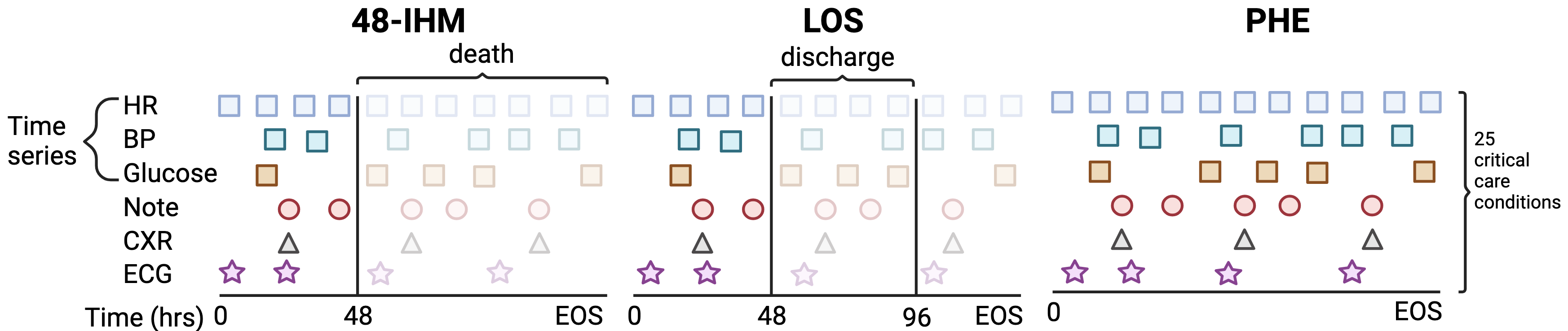
Figure 4: Schematic of tasks of interest. Plotted are example vitals/labs, radiological notes, X-rays, and ECGs sampled over the course of a patient’s ICU stay. The first three rows represent example observations from a single modality consisting of three irregularly sampled vital signs (HR, BP), and lab values (Glucose). The following three rows represent irregularly sampled radiological notes, X-rays, and ECGs. Opaque shapes denote observations falling within the observation window (i.e., observations that are used to generate predictions), while translucent shapes are not used to generate predictions. For the 48-IHM task, we use the first 48 hours of observations to predict death at any time during the ICU stay. For the LOS task, we use the first 48 hours of observations to predict whether the patient will be discharged (alive) during the following 48 hours. And in the phenotyping task (PHE), we use all observations to predict one of 25 critical care conditions.

We implement an in-hospital mortality prediction (48-IHM) task to evaluate our method’s ability to predict short-term patient deterioration. Similarly, an accurate determination of patient discharge times is crucial for optimizing patient outcomes and hospital resource allocation (Bertsimas et al., 2022), which motivates our length-of-stay (LOS) task. We frame 48-IHM and LOS as binary classification problems and use a 48-hour observation window (for patients who spent at least 48 hours in the ICU) to predict in-hospital mortality (48-IHM) and discharge (without expiration) within the 48 hours following the observation window (LOS). Lastly, identifying the presence of specific acute care conditions in patient records is essential for various clinical objectives, including the construction of cohorts for clinical studies and the detection of comorbidities (Agarwal et al., 2016). Traditional methods, often reliant on manual chart reviews or simple billing code-based definitions, are increasingly being supplemented by machine learning techniques (Harutyunyan et al., 2019); automating this process requires high-fidelity classifications, motivating our 25-type phenotype classification (25-PHE) task. In this multilabel classification problem, we attempt to predict one of 25 acute care conditions using data from the entire ICU stay.

Evaluation

In our initial analysis, we focused on patients with no missing modalities, resulting in a dataset comprised of 8,770 ICU stays for the 48-IHM and LOS tasks, and 14,541 stays for the 25-PHE task. For our analyses with missing observations, we include a total of 35,129 stays for 48-IHM and LOS, and 71.173 for 25-PHE. To evaluate the single-label tasks, 48-IHM and LOS, we employ the F1-score and AUROC as our primary metrics. In line with previous studies (Zhang et al., 2023; Lin et al., 2019; Arbabi et al., 2019), we use macro-averaged F1-score and AUROC to assess the 25-PHE task.

A.1 Dataset

We leveraged data from MIMIC-IV (Johnson et al., 2020), a comprehensive database with records from nearly $300k$ patients admitted to a medical center from 2008 to 2019, focusing on the subset of 73,181 ICU stays. We were able to link core ICU records (containing lab results and vital signs) to corresponding chest X-rays (Johnson et al., 2019b), radiological notes (Johnson et al., 2023), and electrocardiogram (ECG) data (Gow et al., 2022) taking place during a given ICU stay. We allocated 70 percent of the data for model training, with the remaining 30 percent evenly split between validation and testing.

A.2 Missingness rates

The total number of samples for each of our three tasks (i.e., those in which at least one vital sign was recorded in the specified observation window), along with the total number of observations per-modality, are shown in Table 5.

Table 5: We present the total number of ICU stays in each task, taking into account observations with missing modalities. The total number of stays with at least one observation of the corresponding modality are shown in the three right-most columns.

Task(s)	Total	Text	CXR	ECG
48-IHM & LOS	35,129	32,038	8,781	18,271
25-PHE	73,173	56,824	14,568	35,925

Appendix B Data Preprocessing

In the preprocessing stage, we focused on 30 pertinent lab and chart events from each patient’s ICU record for vital sign measurements. For chest X-rays, we utilized a pre-trained DenseNet-121 model (Cohen et al., 2022), which was fine-tuned on the CheXpert dataset (Irvin et al., 2019), to extract 1024-dimensional image embeddings. For radiological notes, we obtained 768-dimensional embeddings using the BioClinicalBERT model (Alsentzer et al., 2019). ECG signals were processed using a convolutional autoencoder, adapted from Attia et al. (2019), to generate a 256-dimensional embedding for each ECG.

Time series

We selected 30 time series events for inclusion, following Soenksen et al. (2022). Nine of these were vital signs: heart rate, mean/systolic/diastolic blood pressure, respiratory rate, oxygen saturation, and Glascow Coma Scale (GCS) verbal, eye, and motor response. We also included 21 lab values: potassium, sodium, chloride, creatinine, urea nitrogram, bicarbonate, anion gap, hemoglobin, hematocrit, magnesium, platlet count, phosphate, white blood cell count, total calcium, MCH, red blood cell count, MCHC, MCV, RDW, platlet count, neutrophil count, and vancomycin. We standard scale each time series value to have mean $0$ and standard deviation $1$, based on the values in the training set.

Chest X-rays

To incorporate a medical imaging modality into our analyses, we use the MIMIC-CXR-JPG (Johnson et al., 2019a) module available from Physionet (Goldberger et al., 2000), which includes 377,110 JPG format images derived from the DICOM-based MIMIC-CXR database (Johnson et al., 2019b). Following Soenksen et al. (2022), for each image, we resize each JPG image to 224 $\times$ 224 pixels and then extract embeddings from the last layer of the Densenet121 model. We identify X-rays taken while the patient was in the ICU by first matching subject IDs in MIMIC-CXR-JPG with the core MIMIC-IV database, then limiting these matched X-rays to those with a chart time occuring between an ICU admission and discharge.

Radiological notes

To incorporate text data, we use the MIMIC-IV-Note module (Johnson et al., 2023), which contains 2,321,355 deidentified radiology reports for 237,427 patients that can be matched with patients in the main MIMIC-IV dataset via a similar approach to chest X-rays. We note that we were unable to obtain intermediate clinical notes (i.e., notes made by clinicians throughout a patient stay), as those have not yet been publicly released. We extract note embeddings using Bio-Clinical BERT (Alsentzer et al., 2019).

Electrocardiograms (ECGs)

To include ECGs as an additional modality in our models, we utilize the MIMIC-IV-ECG (Gow et al., 2022) module, which includes approximately 800,000 ECGs (10 seconds, sampled at 500 Hz) collected from nearly 160,000 unique patients. To transform the ECGs so that they are suitable for input to our model, we adopt a convolutional autoencoder approach, adapted from Attia et al. (2019), that compresses each ECG into a 256-dimensional vector. Specifically, each diagnostic ECG contains a $5000\times 12$ dimensional vector (5000 time points $\times$ 12 ECG leads). To prepare the ECG for input to the autoencoder, we only include the first $4096$ time points. We then train the autoencoder to compress the ECG into a 256-dimensional latent vector, and then reconstruct the original ECG using upsampling layers, using mean squared error as our loss function. The architecture is shown in Figure 5.

We train the autoencoder with 90% of the ECGs available in the MIMIC-IV-ECG projection and use the rest for validation. We selected a batch size of 2048, and reduced the learning rate by a factor of $0.5$ is the validation loss had plateaued for $3$ epochs. Training stopped if the validation loss had not decreased for $6$ epochs. For our encoder, we use filter numbers of $[16,16,32,32,64,64]$, kernel widths of $[5,5,5,3,3,3]$ and a dropout rate of $0.1$. For the decoder, we use the same filter numbers and kernel widths in reverse, and maintain a dropout rate of $0.1$.

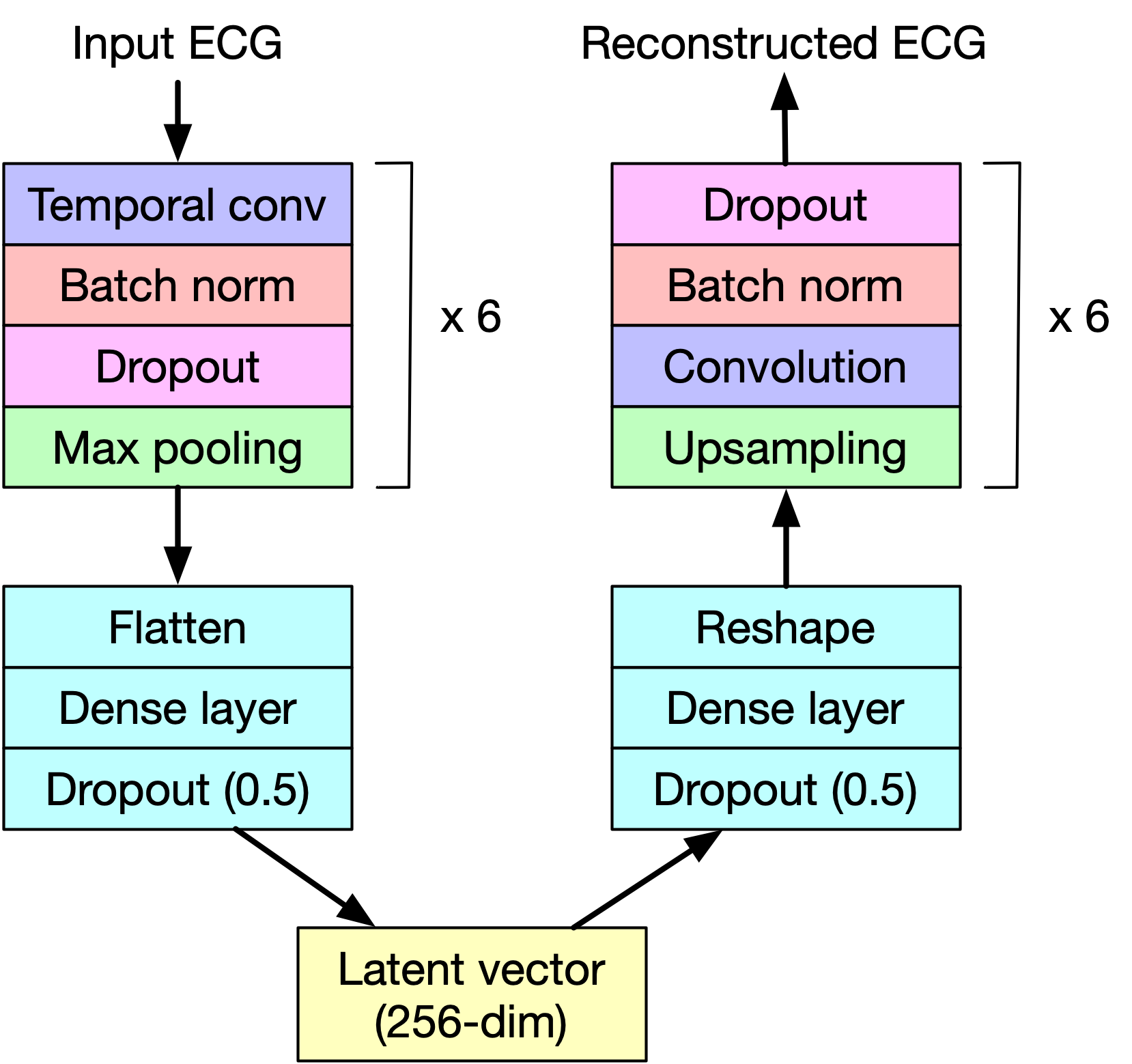
Figure 5: CNN autoencoder architecture. The encoder consists of six convolutional blocks (temporal convolution, batch normalization, dropout, and max pooling layers), followed by a dense layer that reduces the dimensionality of the representation of 256. The decoder then reconstructs the input ECG (dimensionality $4096\times 12$) from this latent vector via a dense layer, followed by six upsampling convolutional blocks (upsampling, convolutional, batch normalization, and dropout layers).

Appendix C Modeling Irregularity

C.1 Unified Temporal Discretization Embeddings

Unlike the embeddings in chest X-rays, clinical notes, and ECGs, vitals/lab values present temporal irregularity across dimensions. That is, for the former three modalities, each dimension of the corresponding is observed at each irregular time point $\bm{\tau}$. By contrast, the sampling for vitals/labs is irregular both within and across dimensions. For example, we might observe heart rate values sampled at times $\bm{\tau}_{\text{HR}}=\{0,0.2,0.8,1.2,2.8\}$ and glucose values sampled at time $\bm{\tau}_{\text{Glu}}=\{0.1,0.7,3.4\}$. Given this unique challenge present in vitals/labs, we adapt the Unified Temporal Discretization Embedding (UTDE) approach described in Zhang et al. (2023), which combines the mTAND approach described in Section 3.2 with a simpler imputation-based discretization scheme. Specifically, given a set of $t$ observations $\mathbf{x}\in\mathbb{R}^{t}$ observed at irregular times $\bm{\tau}\in\mathbb{R}^{t}$, we a simple imputation scheme to discretize $\mathbf{x}$ into target bins $\bm{\gamma}$ (e.g., $\bm{\gamma}=\{0,1,2,...,\gamma\}$. Specifically, given bin value $\gamma_{i}\in\bm{\gamma}$, we apply the following rules:

• If there exists a previously observed value of $\mathbf{x}$ (i.e., $\exists\tau\in\bm{\tau}\,st.\,\tau\leq\gamma_{i}$), we set the imputed value of $\mathbf{x}$ at time $\gamma$, $\hat{x}_{\gamma_{i}}$, to the closest previously observed value.

• If no previously observed value exists, we set the value of $\hat{x}_{\gamma_{i}}$ to the global mean of $\mathbf{x}$.

We do this for each possible vitals/lab, to generate a matrix of imputation embeddings $\mathbf{I}\in\mathbb{R}^{\gamma\times d_{\text{vitals}}}$, were $d_{\text{vitals}}$ is the number of vitals/labs. We then input this embedding into a 1D causal convolutional layer with stride 1 to obtain our final imputation embeddings with hidden dimension $d_{h}$, $\mathbf{E}_{\text{Imp}}\in\mathbb{R}^{\gamma\times d_{h}}$.

C.2 Unifying imputation and mTAND embeddings

We combined simple imputation and mTAND embeddings via a gating function $\mathbf{g}$. Following Zhang et al. (2023), we let $\mathbf{E}_{\text{mTAND}}\in\mathbb{R}^{\gamma\times d_{h}}$ denote the mTAND embeddings for vitals/labs derived from the process described in Section 3.2 and let $\mathbf{E}_{\text{Imp}}\in\mathbb{R}^{\gamma\times d_{h}}$ denote the simple imputations from the process described above. We use each of these discretization embeddings to derive a final set of embeddings for vitals/labs $\mathbf{E}_{\text{vitals}}$ via a one-layer MLP gating function $f$. Specifically, we let $\mathbf{g}=f(\mathbf{E}_{\text{Imp}}\oplus\mathbf{E}_{\text{mTAND}})$, where $\oplus$ denotes the concatenation operator. We then calculate $\mathbf{E}_{\text{vitals}}$ as

$$\mathbf{E}_{\text{vitals}}=\mathbf{g}\odot\mathbf{E}_{\text{Imp}}+(1-\mathbf{g})\odot\mathbf{E}_{\text{mTAND}}\in\mathbb{R}^{\gamma\times d_{h}},$$

where $\odot$ denotes point-wise multiplication.

Appendix D Baseline Comparison

Considering the relatively recent release of MIMIC-IV, there have been limited applications to this dataset. In our study, we evaluated both FuseMoE and various baselines using the earlier MIMIC-III version, as well as on our processed data from MIMIC-IV. To our knowledge, the HAIM approach described in Soenksen et al. (2022) represents the only comprehensive attempt at multimodal modeling on the MIMIC-IV dataset to date.

D.1 MISTS

This approach, from Zhang et al. (2023), casts time series and clinical notes as multivariate, irregularly-sampled time series (MISTS) and uses layers of self- and cross-attention to fuse modalities. The method uses a Time2Vec (Kazemi et al., 2019) encoding scheme to represent the irregularity of observation times. We use the same hyperparameters as in the original paper (e.g., $3$ self- and cross-attention blocks, $128$-dimensional time embedding, etc.).

D.2 MultT

This model from Tsai et al. (2019) relies on multiple stacks of pairwise and bidirectional cross-modal attention blocks (without a self-attention mechanism) to attend to low-level features. The results of cross-modal attention are then sent to modality-specific transformers, concatenated, and used to make predictions.

D.3 MAG

This method introduces the Multimodal Adaptation Gate (MAG) as an extension to BERT and XLNet, allowing these pre-trained models to incorporate visual and acoustic data during fine-tuning. By generating a modality-conditioned shift in their internal representations, MAG enables enhanced sentiment analysis performance on multimodal datasets, achieving human-level accuracy in the field (Rahman et al., 2020).

D.4 TF

The proposed Tensor Fusion approach (TF) integrates three core components: Modality Embedding Subnetworks for generating rich embeddings from unimodal inputs, a Tensor Fusion Layer for capturing all levels of modality interactions through a 3-fold Cartesian product, and a Sentiment Inference Subnetwork tailored to perform sentiment analysis based on the fusion layer’s output (Zadeh et al., 2017).

D.5 HAIM

The multimodal fusion approach detailed by Soenksen et al. (2022) extracts a single set of features for each ICU stay, and uses this to predict the outcome of interest (in-hospital mortality, etc.). For vitals/lab values, the authors extract a set of 11 generic time series features: signal length, maximum, minimum, mean, median, SD, variance, number of peaks, and average time-series slope and piece-wise change over time of these metrics. This is done independently for each of the 30 events, leading to $30\times 11=330$ vital/lab features per ICU stay. To provide a fair comparison with our method, we only include the most recent five notes and $128$ vitals measurements in calculating embeddings. We only include entries for which all modalities are observed. For note/X-ray/ECG embeddings, we compute the mean embedding across all observations occurring during the specified time frame (i.e., first 48 hours of 48-IHM and LOS, the entire stay for PHE). As with our method, we standard scale values based on the training set.

Soenksen et al. (2022) uses an XGBoost (Chen & Guestrin, 2016) classifier to predict the outcomes of interest. We follow the hyperparameter optimization approach described in the paper. Specifically, we conduct a grid search across the following sets of hyperparameters: max depth $=\{5,6,7,8\}$, number of estimators $=\{200,300\}$, learning rate $=\{0.3,0.1,0.05\}$. Hyperparameters are selected based on the maximum AU-ROC from five-fold cross-validation

D.6 Implementation

We integrate D.1 through D.4 into our workflow using the implementation provided by (Zhang et al., 2023). For D.5, we adapt the time series (e.g., series variance, mean, etc.) feature extraction and model fitting code from the repository released by the corresponding paper. The original paper doesn’t use ECG waveforms, so we adopt a similar approach to ECG embeddings as with image and note embeddings, and take the mean value of the latent vector across all included observations.

Table 6: Hyperparameters used for MoE framework and general architecture.

Hyper-Parameter Type	Parameter Name	Value
MoE	Number of experts	16
	FFN hidden size	512
	Top k	4
	Disjoint top k	2
	Hidden activation function	GeLU
	Number of MoE layers	3
Other Parameters	Random seed	[32, 42, 52]
	Training epochs	8
	Training batch size	2
	Eval batch size	8
	CNN kernel size	1
	Gradient accumulation steps	16
	BERT update epochs	2
	BERT learning rate	2.00E-05
	Time series encoder learning rate	4.00E-04
	Number of notes to include for a patient	5
	Get notes from beginning or last	Last
	Attention embedding dimension	128
	Number of attention heads	8
	Maximum time for irregular time series	48
	Time embedding dimension	64

Appendix E Computational Resources and Hyper-Parameters

E.1 Computational resources

We train models using a Lambda Workstation with four A550 GPUs with 24 GB of memory. We are able to train models using a single GPU. An analysis of computation time and memory requirements is shown in Figure 3.

E.2 Hyper-Parameters

All parameters can be found in Table 6 and the codebase submitted in the zip file.

Appendix F Additional Results

Below are additional results on comparing FuseMoE with baselines on the MIMIC-III data (Table 7) that only has vital signs and clinical notes, and the vital signs and CXR of the MIMIC-IV data (Table 8). All experiments are based on the “joint experts and router” configuration. FuseMoE also shows noticeable advantages in these settings.

Table 7: Comparison of FuseMoE-based methods (gray) and baselines, utilizing vital signs and clinical notes of MIMIC-III. The best results are highlighted in bold font, and the second-best results are underlined. All results are averaged across 3 random experiments. Since HAIM is not designed for the MIMIC-III dataset, we use the concatenation method from e.g. Khadanga et al. (2019) as a replacement.

Task $\backslash$ Method				MISTS	MulT	MAG	TF	Concat	Softmax	Gaussian	Laplace
48-IHM	AUROC	89.14 $\pm$ 0.57	87.26 $\pm$ 0.35	86.53 $\pm$ 1.21	87.22 $\pm$ 0.89	86.72 $\pm$ 0.76	90.25 $\pm$ 0.74	90.77 $\pm$ 0.18	91.19 $\pm$ 0.52
	F1	56.45 $\pm$ 1.30	54.13 $\pm$ 1.20	53.20 $\pm$ 2.13	51.44 $\pm$ 0.66	52.77 $\pm$ 0.70	56.41 $\pm$ 0.98	56.21 $\pm$ 0.17	57.36 $\pm$ 0.73
25-PHE	AUROC	86.06 $\pm$ 0.06	85.96 $\pm$ 0.07	85.94 $\pm$ 0.07	84.74 $\pm$ 0.16	85.94 $\pm$ 0.21	86.41 $\pm$ 0.75	85.96 $\pm$ 0.64	86.72 $\pm$ 0.27
	F1	54.84 $\pm$ 0.31	54.20 $\pm$ 0.33	53.73 $\pm$ 0.37	49.84 $\pm$ 0.83	53.30 $\pm$ 0.35	55.02 $\pm$ 0.23	55.29 $\pm$ 0.45	55.38 $\pm$ 0.69

Table 8: Comparison of FuseMoE-based methods (gray) and baselines, utilizing vital signs and CXR of MIMIC-IV. The best results are highlighted in bold font, and the second-best results are underlined. All results are averaged across 3 random experiments.

Task $\backslash$ Method				MISTS	MulT	MAG	TF	HAIM	Softmax	Gaussian	Laplace
48-IHM	AUROC	81.36 $\pm$ 0.24	77.70 $\pm$ 0.44	81.19 $\pm$ 1.25	76.92 $\pm$ 0.65	80.87 $\pm$ 0.00	82.08 $\pm$ 0.26	81.26 $\pm$ 0.18	82.97 $\pm$ 0.49
	F1	43.35 $\pm$ 0.39	28.40 $\pm$ 0.75	39.59 $\pm$ 0.43	46.59 $\pm$ 0.33	40.88 $\pm$ 0.00	38.14 $\pm$ 0.31	44.59 $\pm$ 0.24	47.48 $\pm$ 0.23
LOS	AUROC	82.07 $\pm$ 0.82	81.94 $\pm$ 0.26	81.86 $\pm$ 0.76	81.47 $\pm$ 0.89	81.69 $\pm$ 0.00	82.96 $\pm$ 0.47	82.74 $\pm$ 0.85	83.22 $\pm$ 0.68
	F1	74.07 $\pm$ 0.18	74.46 $\pm$ 0.17	73.89 $\pm$ 0.93	73.39 $\pm$ 0.14	72.93 $\pm$ 0.00	75.67 $\pm$ 0.59	75.16 $\pm$ 0.42	75.43 $\pm$ 0.19
25-PHE	AUROC	71.50 $\pm$ 0.22	71.20 $\pm$ 0.76	70.89 $\pm$ 0.47	70.55 $\pm$ 0.29	63.43 $\pm$ 0.00	71.38 $\pm$ 0.31	70.87 $\pm$ 0.67	71.44 $\pm$ 0.24
	F1	33.52 $\pm$ 0.39	32.80 $\pm$ 0.18	33.14 $\pm$ 0.61	33.56 $\pm$ 0.74	42.45 $\pm$ 0.00	33.49 $\pm$ 0.15	31.94 $\pm$ 0.09	34.13 $\pm$ 0.56

Appendix G Exact-Specified Setting

In this appendix, we study the theoretical behaviors of the MLE under the exact-specified setting, i.e., $k=k_{*}$, of the Laplace gating Gaussian MoE. We demonstrate that under the exact-specified setting, the rate of estimated conditional density function $p_{\widehat{G}_{n}}$ to $p_{G_{*}}$ is parametric $O(n^{-1/2})$ (up to some logarithmic factor).

Theorem G.1.

The density estimation $p_{\widehat{G}_{n}}(Y|X)$ converges to the true density $p_{G_{*}}(Y|X)$ under the Total Variation distance $V$ at the following rate:

$$\mathbb{E}_{X}[V(p_{\widehat{G}_{n}}(\cdot|X),p_{G_{*}}(\cdot|X))]=\mathcal{O}(\sqrt{\log(n)/n}).$$

Proof of Theorem G.1 is in Appendix H.1. The result of Theorem G.1 indicates that as long as we can establish the lower bound of the total variation distance between $p_{\widehat{G}_{n}}$ and $p_{G_{*}}$ based on certain loss function between the MLE $\widehat{G}_{n}$ and the true mixing measure $G_{*}$, we directly achieve the rate of the MLE under that loss function.

Voronoi Loss We now define that loss function between the MLE and the true mixing measure. Given some mixing measure $G:=\sum_{i=1}^{k}\exp(\beta_{i})\delta_{(W_{i},a_{i},b_{i},\nu_{i})}$, we distribute its components to the following Voronoi cells which are generated by the support of the true mixing measure $G_{*}:=\sum_{j=1}^{k_{*}}\exp(\beta_{j}^{*})\delta_{(W_{j}^{*},a_{j}^{*},b_{j}^{*},\nu_{j}^{*})}$:

$$\mathcal{A}_{j}\equiv\mathcal{A}_{j}(G):=\{i\in[k]:\|\theta_{i}-\theta^{*}_{j}\|\leq\|\theta_{i}-\theta^{*}_{\ell}\|,\ \forall\ell\neq j\},$$

where $\theta_{i}:=(W_{i},a_{i},b_{i},\nu_{i})$ and $\theta^{*}_{j}:=(W_{j}^{*},a_{j}^{*},b_{j}^{*},\nu_{j}^{*})$ for any $1\leq i\leq k$ and $1\leq j\leq k_{*}$. Based on these Voronoi cells, we propose the following Voronoi loss function for the exact-specified setting:

$$\mathcal{D}_{1}(G,G_{*}):=\max\Bigg{[}\Big{|}\sum_{i\in\mathcal{A}_{\tau_{j}}}\exp(\beta_{i})-\exp(\beta^{*}_{\tau_{j}})\Big{|}+\sum_{j\in[K]:|\mathcal{A}_{j}|=1}\sum_{i\in\mathcal{A}_{\tau_{j}}}\exp(\beta_{i})\Phi_{i\tau_{j}}(1,1,1,1)\Bigg{]},$$ (10)

where the maximum in the definition of Voronoi loss function $\mathcal{D}_{1}$ is for $\{\tau_{1},\tau_{2},\ldots,\tau_{K}\}\subseteq[k_{*}]$. Furthermore, for any $(\rho_{1},\rho_{2},\rho_{3},\rho_{4})\in\mathbb{R}^{4}$, we define $\Phi_{i\tau_{j}}(\rho_{1},\rho_{2},\rho_{3},\rho_{4})=\|W_{i}-W_{\tau_{j}}^{*}\|^{\rho_{1}}+\|a_{i}-a_{\tau_{j}}^{*}\|^{\rho_{2}}+|b_{i}-b_{\tau_{j}}^{*}|^{\rho_{3}}+|\nu_{i}-\nu_{\tau_{j}}^{*}|^{\rho_{4}}$ for any $i\in\mathcal{A}_{\tau_{j}}$ and $j\in[K]$. We demonstrate in the following theorem that the rate of MLE to the true mixing measure under the Voronoi loss function $\mathcal{D}_{1}$ is $\mathcal{O}(n^{-1/2})$ (up to some logarithmic factor).

Theorem G.2 (Exact-specified setting).

When $k=k_{*}$ is known, the following Total Variation bound holds guarantetrue for any $G\in\mathcal{G}_{k}(\Theta)$:

$$\mathbb{E}_{X}[V(p_{G}(\cdot|X),p_{G_{*}}(\cdot|X))]\gtrsim\mathcal{D}_{1}(G,G_{*}).$$

Therefore, we have $\mathcal{D}_{1}(\widehat{G}_{n},G_{*})=\mathcal{O}(\sqrt{\log(n)/n})$.

Proof of Theorem G.2 is in Appendix H.2. The convergence rate of MLE under the Voronoi loss function $\mathcal{D}_{1}$ implies that the rates of estimating the true parameters $W_{i}^{*},a_{i}^{*},b_{i}^{*},\nu_{i}^{*}$ are also $\mathcal{O}(n^{-1/2})$ (up to logarithmic factors). These rates are comparable to those under the exact-specified setting of softmax gating Gaussian MoE (cf. Theorem 1 in  (Nguyen et al., 2023b)).

Appendix H Proof of Theoretical Results

In this appendix, we provide proofs for all theoretical results in the paper. Throughout this appendix, for any vector $v\in\mathbb{R}^{d}$ and $\alpha:=(\alpha_{1},\alpha_{2},\ldots,\alpha_{d})\in\mathbb{N}^{d}$, we denote $v^{\alpha}=v_{1}^{\alpha_{1}}v_{2}^{\alpha_{2}}\ldots v_{d}^{\alpha_{d}}$, $|v|:=v_{1}+v_{2}+\ldots+v_{d}$ and $\alpha!:=\alpha_{1}!\alpha_{2}!\ldots\alpha_{d}!$.

H.1 Proof of Theorem G.1

In this appendix, we employ results for M-estimators in (van de Geer, 2000) to establish the density estimation rate under the top-K sparse Laplace gating Gaussian mixture of experts (MoE).

Firstly, we introduce some necessary notations and fundamental results. In particular, let $\mathcal{P}_{k_{*}}(\Theta):=\{p_{G}(Y|X):G\in\mathcal{G}_{k_{*}}(\Omega)\}$ be the set of all conditional density functions w.r.t mixing measures in $\mathcal{G}_{k_{*}}(\Omega)$. Next, we denote by $N(\varepsilon,\mathcal{P}_{k_{*}}(\Omega),\|\cdot\|_{1})$ the covering number of metric space $(\mathcal{P}_{k_{*}}(\Omega),\|\cdot\|_{1})$. Meanwhile, $H_{B}(\varepsilon,\mathcal{P}_{k_{*}}(\Omega),h)$ stands for the bracketing entropy of $\mathcal{P}_{k_{*}}(\Omega)$ under the Hellinger distance $h$ where $h(p,q):=\Big{(}\frac{1}{2}\int(\sqrt{p}-\sqrt{q})^{2}d\mu\Big{)}^{1/2}$ for any probability densities $p,q$ dominated by the Lebesgue measure $\mu$. Then, we provide in the following lemma the upper bounds of those terms.

Lemma H.1.

If $\Omega$ is a bounded set, then the following inequalities hold for any $0<\eta<1/2$:

• $\log N(\eta,\mathcal{P}_{k_{*}}(\Omega),\|\cdot\|_{1})\lesssim\log(1/\eta)$;

• $H_{B}(\eta,\mathcal{P}_{k_{*}}(\Omega),h)\lesssim\log(1/\eta)$.

Proof of Lemma H.1 is in Appendix H.1.2. Subsequently, we denote

$$\widetilde{\mathcal{P}}_{k_{*}}(\Omega) :=\{p_{(G+G_{*})/2}(Y|X):G\in\mathcal{G}_{k_{*}}(\Omega)\};$$

$$\widetilde{\mathcal{P}}^{1/2}_{k_{*}}(\Omega) :=\{p^{1/2}_{(G+G_{*})/2}(Y|X):G\in\mathcal{G}_{k_{*}}(\Omega)\}.$$

In addition, for each $\delta>0$, we define a Hellinger ball centered around the conditional density function $p_{G_{*}}(Y|X)$ and intersected with the set $\widetilde{\mathcal{P}}^{1/2}_{k_{*}}(\Omega)$ as

$$\widetilde{\mathcal{P}}^{1/2}_{k_{*}}(\Omega,\delta):=\{p^{1/2}\in\widetilde{\mathcal{P}}^{1/2}_{k_{*}}(\Omega):h(p,p_{G_{*}})\leq\delta\}.$$

To capture the size of the above Hellinger ball, (van de Geer, 2000) suggest using the following quantity:

$$\mathcal{J}_{B}(\delta,\widetilde{\mathcal{P}}^{1/2}_{k_{*}}(\Omega,\delta)):=\int_{\delta^{2}/2^{13}}^{\delta}H^{1/2}_{B}(t,\widetilde{\mathcal{P}}^{1/2}_{k_{*}}(\Omega,t),\|\cdot\|)\mathrm{d}t\vee\delta,$$ (11)

where $t\vee\delta:=\max\{t,\delta\}$. Given those notations, let us recall a standard result for density estimation in (van de Geer, 2000).

Lemma H.2 (Theorem 7.4, (van de Geer, 2000)).

Take $\Psi(\delta)\geq\mathcal{J}_{B}(\delta,\widetilde{\mathcal{P}}^{1/2}_{k_{*}}(\Omega,\delta))$ such that $\Psi(\delta)/\delta^{2}$ is a non-increasing function of $\delta$. Then, for some sequence $(\delta_{n})$ and universal constant $c$ which satisfy $\sqrt{n}\delta^{2}_{n}\geq c\Psi(\delta)$, we obtain that

$$\mathbb{P}\left(\mathbb{E}_{X}\Big{[}h(p_{\widehat{G}_{n}}(\cdot|X),p_{G_{*}}(\cdot|X))\Big{]}>\delta\right)\leq c\exp(-n\delta^{2}/c^{2}),$$

for any $\delta\geq\delta_{n}$

Proof of Lemma H.2 can be found in (van de Geer, 2000). Now, we are ready to provide the proof for convergence rate of density estimation in Theorem G.1 in Appendix H.1.1.

H.1.1 Main Proof

It is worth noting that for any $t>0$, we have

$$H_{B}(t,\widetilde{\mathcal{P}}^{1/2}_{k_{*}}(\Omega,t),\|\cdot\|)\leq H_{B}(t,\mathcal{P}_{k_{*}}(\Omega,t),h).$$

Then, the integral in equation 11 is upper bounded as follows:

$$\mathcal{J}_{B}(\delta,\widetilde{\mathcal{P}}^{1/2}_{k_{*}}(\Omega,\delta))\leq\int_{\delta^{2}/2^{13}}^{\delta}H^{1/2}_{B}(t,\mathcal{P}_{k_{*}}(\Omega,t),h)\mathrm{d}t\vee\delta\lesssim\int_{\delta^{2}/2^{13}}^{\delta}\log(1/t)\mathrm{d}t\vee\delta,$$ (12)

where the second inequality follows from part (ii) of Lemma H.1.

As a result, by choosing $\Psi(\delta)=\delta\cdot\sqrt{\log(1/\delta)}$, we can verify that $\Psi(\delta)/\delta^{2}$ is a non-increasing function of $\delta$. Furthermore, the inequality in equation 12 indicates that $\Psi(\delta)\geq\mathcal{J}_{B}(\delta,\widetilde{\mathcal{P}}^{1/2}_{k_{*}}(\Omega,\delta))$. Next, let us consider a sequence $(\delta_{n})$ defined as $\delta_{n}:=\sqrt{\log(n)/n}$. This sequence can be validated to satisfy the condition $\sqrt{n}\delta_{n}^{2}\geq c\Psi(\delta)$ for some universal constant $c$. Therefore, by Lemma H.2, we reach the conclusion of Theorem G.1:

$$\mathbb{P}\Big{(}\mathbb{E}_{X}[h(p_{\widehat{G}_{n}}(\cdot|X),p_{G_{*}}(\cdot|X))]>C\sqrt{\log(n)/n}\Big{)}\lesssim n^{-c},$$

for some universal constant $C$ depending only on $\Omega$.

H.1.2 Proof of Lemma H.1

Part (i). In this part, we will derive the following upper bound for the covering number of metric space $(\mathcal{P}_{k_{*}}(\Omega),\|\cdot\|_{1})$ for any $0<\eta<1/2$ given the bounded set $\Omega$:

$$\log N(\eta,\mathcal{P}_{k_{*}}(\Omega),\|\cdot\|_{1})\lesssim\log(1/\eta).$$

To start with, we denote $\Theta:=\{(a,b,\nu)\in\mathbb{R}^{d}\times\mathbb{R}\times\mathbb{R}_{+}:(\beta,W,a,b,\nu)\in\Omega\}$. As $\Omega$ is a bounded set, the set $\Theta$ is also bounded. Therefore, we can find an $\eta$-cover of $\Theta$, denoted by $\overline{\Theta}_{\eta}$. Additionally, we also define $\Delta:=\{(\beta,W)\in\mathbb{R}\times\mathbb{R}^{d}:(\beta,W,a,b,\nu)\in\Omega\}$, and $\overline{\Delta}_{\eta}$ be an $\eta$-cover of $\Delta$. Then, it can be validated that

$$|\overline{\Theta}_{\eta}|\leq\mathcal{O}(\eta^{-(d+2)k_{*}}),\quad|\overline{\Delta}_{\eta}|\leq\mathcal{O}(\eta^{-(d+1)k_{*}}).$$

Next, for each mixing measure $G=\sum_{i=1}^{k_{*}}\exp(\beta_{i})\delta_{(W_{i},a_{i},b_{i},\nu_{i})}\in\mathcal{G}_{k_{*}}(\Omega)$, we take into account two other mixing measures. The first measure is $G^{\prime}=\sum_{i=1}^{k_{*}}\exp(\beta_{i})\delta_{(W_{i},\overline{a}_{i},\overline{b}_{i},\overline{\nu}_{i})}$, where $(\overline{a}_{i},\overline{b}_{i},\overline{\nu}_{i})\in\overline{\Theta}_{\eta}$ is the closest points to $(a_{i},b_{i},\nu_{i})$ in this set for all $i\in[k_{*}]$. The second one is $\overline{G}:=\sum_{i=1}^{k_{*}}\exp(\overline{\beta}_{i})\delta_{(\overline{W}_{i},\overline{a}_{i},\overline{b}_{i},\overline{\nu}_{i})}$ in which $(\overline{\beta}_{i},\overline{W}_{i})\in\overline{\Delta}_{\eta}$ for any $i\in[k_{*}]$. Next, let us define

$$\mathcal{T}:=\{p_{\overline{G}}\in\mathcal{P}_{k_{*}}(\Omega):(\overline{\beta}_{i},\overline{W}_{i})\in\overline{\Delta}_{\eta},\ (\overline{a}_{i},\overline{b}_{i},\overline{\nu}_{i})\in\overline{\Theta}_{\eta},\forall i\in[k_{*}]\},$$

then it is obvious that $p_{\overline{G}}\in\mathcal{T}$. Now, we will show that $\mathcal{T}$ is an $\eta$-cover of metric space $(\mathcal{P}_{k_{*}}(\Omega),\|\cdot\|_{1})$ with a note that it is not necessarily the smallest cover. Indeed, according to the triangle inequality,

$$\|p_{G}-p_{\overline{G}}\|_{1}\leq\|p_{G}-p_{G^{\prime}}\|_{1}+\|p_{G^{\prime}}-p_{\overline{G}}\|_{1}.$$ (13)

Since the softmax function is no greater than one, the first term in the right hand side can be upper bounded as follows:

$$\|p_{G}-p_{G^{\prime}}\|_{1} \leq\sum_{i=1}^{k_{*}}\int\Big{|}f(Y|a_{i}^{\top}X+b_{i},\nu_{i})-f(Y|\overline{a}_{i}^{\top}X+\overline{b}_{i},\overline{\nu}_{i})\Big{|}\mathrm{d}(X,Y)$$

$$\lesssim\sum_{i=1}^{k_{*}}\int\Big{(}\|a_{i}-\overline{a}_{i}\|+\|b_{i}-\overline{b}_{i}\|+\|\nu_{i}-\overline{\nu}_{i}\|\Big{)}\mathrm{d}(X,Y)$$

$$=\sum_{i=1}^{k_{*}}\Big{(}\|a_{i}-\overline{a}_{i}\|+\|b_{i}-\overline{b}_{i}\|+\|\nu_{i}-\overline{\nu}_{i}\|\Big{)}$$

$$\lesssim\eta.$$ (14)

Subsequently, we show that $\|p_{G^{\prime}}-p_{\overline{G}}\|_{1}\lesssim\eta$. For that purpose, we consider $q:=\binom{k_{*}}{K}$ $K$-element subsets of $\{1,\ldots,k_{*}\}$, which are assumed to take the form $\{\tau_{1},\tau_{2},\ldots,\tau_{K}\}$ for any $\tau\in[q]$. Additionally, we also denote $\{\tau_{K+1},\ldots,\tau_{k_{*}}\}:=\{1,\ldots,k_{*}\}\setminus\{\tau_{1},\ldots,\tau_{K}\}$ for any $\tau\in[q]$. Then, we define

$$\mathcal{X}_{\tau} :=\{x\in\mathcal{X}:-\|W_{i}-x\|\geq-\|W_{i^{\prime}}-x\|:i\in\{\tau_{1},\ldots,\tau_{K}\},i^{\prime}\in\{\tau_{K+1},\ldots,\tau_{k_{*}}\}\},$$

$$\widetilde{\mathcal{X}}_{\tau} :=\{x\in\mathcal{X}:-\|\overline{W}_{i}-x\|\geq-\|\overline{W}_{i^{\prime}}-x\|:i\in\{\tau_{1},\ldots,\tau_{K}\},i^{\prime}\in\{\tau_{K+1},\ldots,\tau_{k_{*}}\}\}.$$

By using the same arguments as in the proof of Lemma I.1 in Appendix I, we achieve that either $\mathcal{X}_{\tau}=\widetilde{\mathcal{X}}_{\tau}$ or $\mathcal{X}_{\tau}$ has measure zero for any $\tau\in[q]$. As the $\mathrm{softmax}$ function is differentiable, it is a Lipschitz function with some Lipschitz constant $L\geq 0$. Next, we denote

$$\pi_{{\tau}}(X):=\Big{(}-\|W_{\tau_{i}}-X\|+\beta_{{\tau}_{i}}\Big{)}_{i=1}^{{K}};\qquad\overline{\pi}_{{\tau}}(X):=\Big{(}-\|\overline{W}_{{\tau}_{i}}-X\|+\overline{\beta}_{{\tau}_{i}}\Big{)}_{i=1}^{{K}},$$

for any ${K}$-element subset $\{{\tau}_{1},\ldots{\tau}_{K}\}$ of $\{1,\ldots,k_{*}\}$. Then, we get

$$\|\mathrm{softmax}(\pi_{{\tau}}(X))-\mathrm{softmax}(\overline{\pi}_{{\tau}}(X))\| \leq L\cdot\|\pi_{{\tau}}(X)-\overline{\pi}_{{\tau}}(X)\|$$

$$\leq L\cdot\sum_{i=1}^{{K}}\Big{(}\Big{|}\|W_{{\tau}_{i}}-X\|-\|\overline{W}_{{\tau}_{i}}-X\|\Big{|}+|\beta_{{\tau}_{i}}-\overline{\beta}_{{\tau}_{i}}|\Big{)}$$

$$\leq L\cdot\sum_{i=1}^{{K}}\Big{(}\|W_{{\tau}_{i}}-\overline{W}_{{\tau}_{i}}\|+|\beta_{{\tau}_{i}}-\overline{\beta}_{{\tau}_{i}}|\Big{)}$$

$$\leq L\cdot\sum_{i=1}^{{K}}\Big{(}\eta+\eta\Big{)}$$

$$\lesssim\eta.$$

Back to the proof for $\|p_{G^{\prime}}-p_{\overline{G}}\|_{1}\lesssim\eta$, it follows from the above results that

$$\|p_{G^{\prime}}-p_{\overline{G}}\|_{1} =\int|p_{G^{\prime}}(Y|X)-p_{\overline{G}}(Y|X)|~{}\mathrm{d}(X,Y)$$

$$\leq\sum_{\tau=1}^{q}\int_{\mathcal{X}_{\tau}\times\mathcal{Y}}|p_{G^{\prime}}(Y|X)-p_{\overline{G}}(Y|X)|~{}\mathrm{d}(X,Y)$$

$$\leq\sum_{\tau=1}^{q}\int_{\mathcal{X}_{\tau}\times\mathcal{Y}}\sum_{i=1}^{K}\Big{|}\mathrm{softmax}(\pi_{\tau}(X)_{i})-\mathrm{softmax}(\overline{\pi}_{\tau}(X)_{i})\Big{|}\cdot\Big{|}f(Y|\overline{a}_{\tau_{i}}^{\top}X+\overline{b}_{\tau_{i}},\overline{\nu}_{\tau_{i}})\Big{|}~{}\mathrm{d}(X,Y)$$

$$\lesssim\eta,$$ (15)

It follows from the results in equation 13, equation 14 and equation 15 that $\|p_{G}-p_{\overline{G}}\|_{1}\lesssim\eta$. This result indicates that $\mathcal{T}$ is an $\eta$-cover of the metric space $(\mathcal{P}_{k_{*}}(\Omega),\|\cdot\|_{1})$. As a consequence, we obtain that

$$N(\eta,\mathcal{P}_{k_{*}}(\Omega),\|\cdot\|_{1})\lesssim|\overline{\Delta}_{\eta}|\times|\overline{\Theta}_{\eta}|\leq\mathcal{O}(1/\eta^{(2d+3)k}),$$

which leads to the conclusion of this part: $\log N(\eta,\mathcal{P}_{k_{*}}(\Omega),\|\cdot\|_{1})\lesssim\log(1/\eta)$.

Part (ii). In this part, we provide an upper bound for the bracketing entropy of $\mathcal{P}_{k_{*}}(\Omega)$ under the Hellinger distance $h$:

$$H_{B}(\eta,\mathcal{P}_{k_{*}}(\Omega),h)\lesssim\log(1/\eta).$$

Since $\Omega$ and $\mathcal{X}$ are bounded sets, there exist positive constants $\gamma,\ell,u$ such that $-\gamma\leq a^{\top}X+b\leq\gamma$ and $\ell\leq\nu\leq u$. Let us define

$$B(Y|X):=\begin{cases}\frac{1}{\sqrt{2\pi\ell}}\exp\Big{(}-\frac{Y^{2}}{8u}\Big{)},\quad\text{for }|Y|\geq 2\gamma\\ \frac{1}{\sqrt{2\pi\ell}},\hskip 68.28644pt\text{for }|Y|<2\gamma\end{cases}$$

Then, it can be validated that $f(Y|a^{\top}X+b,\nu)\leq B(Y|X)$ for any $(X,Y)\in\mathcal{X}\times\mathcal{Y}$.

Next, let $\zeta\leq\eta$ which will be chosen later and $\{p_{1},\ldots,p_{N}\}$ be an $\zeta$-cover of metric space $(\mathcal{P}_{k_{*}}(\Omega),\|\cdot\|_{1})$ with the covering number $N:=N(\tau,\mathcal{P}_{k_{*}}(\Omega),\|\cdot\|_{1})$. Additionally, we also consider brackets of the form $[\Psi_{i}^{L}(Y|X),\Psi_{i}^{U}(Y|X)]$ where

$$\Psi_{i}^{L}(Y|X) :=\max\{p_{i}(Y|X)-\tau,0\}$$

$$\Psi_{i}^{U}(Y|X) :=\max\{p_{i}(Y|X)+\tau,B(Y|X)\}.$$

Then, we can check that $\mathcal{P}_{k_{*}}(\Omega)\subseteq\bigcup_{i=1}^{N}[\Psi_{i}^{L}(Y|X),\Psi_{i}^{U}(Y|X)]$ and $\Psi_{i}^{U}(Y|X)-\Psi_{i}^{L}(Y|X)\leq\min\{2\eta,B(Y|X)\}$.

Let $S:=\max\{2\gamma,\sqrt{8u}\}\log(1/\zeta)$, we have for any $i\in[N]$ that

$$\|\Psi_{i}^{U}-\Psi_{i}^{L}\|_{1} =\int_{|Y|<2\gamma}[\Psi_{i}^{U}(Y|X)-\Psi_{i}^{L}(Y|X)]~{}\mathrm{d}X\mathrm{d}Y+\int_{|Y|\geq 2\gamma}[\Psi_{i}^{U}(Y|X)-\Psi_{i}^{L}(Y|X)]~{}\mathrm{d}X\mathrm{d}Y$$

$$\leq S\zeta+\exp\Big{(}-\frac{S^{2}}{2u}\Big{)}\leq S^{\prime}\zeta,$$

where $S^{\prime}$ is some positive constant. This inequality indicates that

$$H_{B}(S^{\prime}\zeta,\mathcal{P}_{k_{*}}(\Omega),\|\cdot\|_{1})\leq\log N(\zeta,\mathcal{P}_{k_{*}}(\Omega),\|\cdot\|_{1})\leq\log(1/\tau).$$

By setting $\zeta=\eta/S^{\prime}$, we obtain that $H_{B}(\eta,\mathcal{P}_{k_{*}}(\Omega),\|\cdot\|_{1})\lesssim\log(1/\eta)$. Finally, since the norm $\|\cdot\|_{1}$ is upper bounded by the Hellinger distance, we reach the conclusion of this part:

$$H_{B}(\eta,\mathcal{P}_{k_{*}}(\Omega),h)\lesssim\log(1/\eta).$$

Hence, the proof is completed.

H.2 Proof of Theorem G.2

First of all, we need to establish the following bound:

$$\mathbb{E}_{X}[V(p_{G}(\cdot|X),p_{G_{*}}(\cdot|X))]\gtrsim\mathcal{D}_{1}(G,G_{*}).$$

For that sake, it is sufficient to demonstrate two following inequalities:

• Inequality A. $\inf_{G\in\mathcal{G}_{k_{*}}(\Omega):\mathcal{D}_{1}(G,G_{*})\leq\varepsilon^{\prime}}\dfrac{\mathbb{E}_{X}[V(p_{G}(\cdot|X),p_{G_{*}}(\cdot|X))]}{\mathcal{D}_{1}(G,G_{*})}>0$;

• Inequality B. $\inf_{G\in\mathcal{G}_{k_{*}}(\Omega):\mathcal{D}_{1}(G,G_{*})>\varepsilon^{\prime}}\dfrac{\mathbb{E}_{X}[V(p_{G}(\cdot|X),p_{G_{*}}(\cdot|X))]}{\mathcal{D}_{1}(G,G_{*})}>0$,

for some constant $\varepsilon^{\prime}>0$.

Proof of inequality A: The inequality A is equivalent to

$$\lim_{\varepsilon\to 0}\inf_{G\in\mathcal{G}_{k_{*}}(\Omega):\mathcal{D}_{1}(G,G_{*})\leq\varepsilon}\frac{\mathbb{E}_{X}[V(p_{G}(\cdot|X),p_{G_{*}}(\cdot|X))]}{\mathcal{D}_{1}(G,G_{*})}>0.$$

Assume that the above inequality is not true, then, there exists a sequence of mixing measure $G_{n}:=\sum_{i=1}^{k_{*}}\exp(\beta^{n}_{i})\delta_{(W_{i}^{n},a_{i}^{n},b_{i}^{n},\nu_{i}^{n})}\in\mathcal{G}_{k_{*}}(\Omega)$ such that both $\mathcal{D}_{1}(G_{n},G_{*})$ and $\mathbb{E}_{X}[V(p_{G_{n}}(\cdot|X),p_{G_{*}}(\cdot|X))]/\mathcal{D}_{1}(G_{n},G_{*})$ go to zero as $n\to\infty$. Now, we define

$$\mathcal{A}^{n}_{j}=\mathcal{A}_{j}(G_{n}):=\{i\in[k_{*}]:\|\theta^{n}_{i}-\theta^{*}_{j}\|\leq\|\theta^{n}_{i}-\theta^{*}_{\tau}\|,\ \forall\tau\neq j\},$$

for any $j\in[k_{*}]$ as Voronoi cells with respect to the mixing measure $G_{n}$, where we denote $\theta^{n}_{i}:=(W_{i}^{n},a_{i}^{n},b_{i}^{n},\nu_{i}^{n})$ and $\theta^{*}_{j}:=(W_{j}^{*},a_{j}^{*},b_{j}^{*},\nu_{j}^{*})$. In this proof, since our arguments are assymptotic, we can assume without loss of generality (WLOG) that these Voronoi cells does not depend on $n$, that is, $\mathcal{A}_{j}=\mathcal{A}^{n}_{j}$. Next, it follows from the hypothesis $\mathcal{D}_{1n}:=\mathcal{D}_{1}(G_{n},G_{*})\to 0$ as $n\to\infty$ that each Voronoi cell contains only one element. Therefore, we may assume WLOG that $\mathcal{A}_{j}=\{j\}$ for any $j\in[k_{*}]$, which implies that $(W_{j}^{n},a_{j}^{n},b_{j}^{n},\nu_{j}^{n})\to(W_{j}^{*},a_{j}^{*},b_{j}^{*},\nu_{j}^{*})$ and $\exp(\beta^{n}_{j})\to\exp(\beta_{j}^{*})$ as $n\to\infty$.

Subsequently, to specify the top $K$ selection in the formulations of $p_{G_{n}}(Y|X)$ and $p_{G_{*}}(Y|X)$, we divide the covariate space $\mathcal{X}$ into some subsets in two ways. In particular, we first consider $q:=\binom{k_{*}}{K}$ different $K$-element subsets of $[k_{*}]$, which are assumed to take the form $\{\tau_{1},\ldots,\tau_{K}\}$, for $\tau\in[q]$. Additionally, we denote $\{\tau_{K+1},\ldots,\tau_{k_{*}}\}:=[k_{*}]\setminus\{\tau_{1},\ldots,\tau_{K}\}$. Then, we define for each $\tau\in[q]$ two following subsets of $\mathcal{X}$:

$$\mathcal{X}^{n}_{\tau}:=\Big{\{}x\in\mathcal{X}:-\|W_{j}-x\|\geq-\|W_{j^{\prime}}-x\|:\forall j\in\{\tau_{1},\ldots,\tau_{K}\},j^{\prime}\in\{\tau_{K+1},\ldots,\tau_{k_{*}}\}\Big{\}},$$

$$\mathcal{X}^{*}_{\tau}:=\Big{\{}x\in\mathcal{X}:-\|W^{*}_{j}-x\|\geq-\|W^{*}_{j^{\prime}}-x\|:\forall j\in\{\tau_{1},\ldots,\tau_{K}\},j^{\prime}\in\{\tau_{K+1},\ldots,\tau_{k_{*}}\}\Big{\}}.$$

Since $(W_{j}^{n},\beta^{n}_{j})\to(W_{j}^{*},\beta_{j}^{*})$ as $n\to\infty$ for any $j\in[k_{*}]$, we have for any arbitrarily small $\eta_{j}>0$ that $\|W_{j}^{n}-W_{j}^{*}\|\leq\eta_{j}$ and $|\beta^{n}_{j}-\beta_{j}^{*}|\leq\eta_{j}$ for sufficiently large $n$. By applying Lemma I.1, we obtain that $\mathcal{X}^{n}_{\tau}=\mathcal{X}^{*}_{\tau}$ for any $\tau\in[q]$ for sufficiently large $n$.

WLOG, we assume that

$$\mathcal{D}_{1}(G_{n},G_{*})=\sum_{i=1}^{K}\Big{[}\exp(\beta_{i}^{n})\Big{(}\|\Delta W_{i}^{n}\|+\|\Delta a_{i}^{n}\|+\|\Delta b_{i}^{n}\|+\|\Delta\nu_{i}^{n}\|\Big{)}+\Big{|}\exp(\beta_{i}^{n})-\exp(\beta_{i}^{*})\Big{|}\Big{]},$$

where we denote $\Delta\beta^{n}_{1i}:=\beta^{n}_{1i}-\beta^{*}_{1i}$, $\Delta a^{n}_{i}:=a^{n}_{i}-a^{*}_{i}$, $\Delta b^{n}_{i}:=b^{n}_{i}-b^{*}_{i}$ and $\Delta\nu^{n}_{i}:=\nu^{n}_{i}-\nu^{*}_{i}$.

Let $\tau\in[q]$ such that $\{\tau_{1},\ldots,\tau_{K}\}=\{1,\ldots,K\}$. Then, for almost surely $(X,Y)\in\mathcal{X}^{*}_{\tau}\times\mathcal{Y}$, we can rewrite the conditional densities $p_{G_{n}}(Y|X)$ and $p_{G_{*}}(Y|X)$ as

$$p_{G_{n}}(Y|X) =\sum_{i=1}^{K}\frac{\exp(-\|W_{i}^{n}-X\|+\beta_{i}^{n})}{\sum_{j=1}^{K}\exp(-\|W_{j}^{n}-X\|+\beta^{n}_{j})}\cdot f(Y|(a_{i}^{n})^{\top}X+b_{i}^{n},\nu_{i}^{n}),$$

$$p_{G_{*}}(Y|X) =\sum_{i=1}^{K}\frac{\exp(-\|W_{i}^{*}-X\|+\beta_{i}^{*})}{\sum_{j=1}^{K}\exp(-\|W_{j}^{*}-X\|+\beta_{j}^{*})}\cdot f(Y|(a_{i}^{*})^{\top}X+b_{i}^{*},\nu_{i}^{*}).$$

Now, we break the rest of our arguments into three steps:

Stage 1 - Density decomposition:

In this step, we aim to decompose the term $Q_{n}:=\Big{[}\sum_{i=1}^{K}\exp(-\|W_{i}^{*}-X\|+\beta_{i}^{*})\Big{]}\cdot[p_{G_{n}}(Y|X)-p_{G_{*}}(Y|X)]$, which can be represented as follows:

$$Q_{n} =\sum_{i=1}^{K}\exp(\beta_{i}^{n})\Big{[}F(Y|X;W_{i}^{n},a_{i}^{n},b_{i}^{n},\nu_{i}^{n})-F(Y|X;W_{i}^{*},a_{i}^{*},b_{i}^{*},\nu_{i}^{*})\Big{]}$$

$$-\sum_{i=1}^{K}\exp(\beta_{i}^{n})\Big{[}H(Y|X;W_{i}^{n})-H(Y|X;W_{i}^{*})\Big{]}$$

$$+\sum_{i=1}^{K}\Big{[}\exp(\beta_{i}^{n})-\exp(\beta_{i}^{*})\Big{]}\Big{[}F(Y|X;W_{i}^{*},a_{i}^{*},b_{i}^{*},\nu_{i}^{*})-H(Y|X,W_{i}^{*})\Big{]}$$

$$: =A_{n}-B_{n}+E_{n},$$ (16)

where we denote $F(Y|X;W,a,b,\nu):=\exp(-\|W-X\|)f(Y|a^{\top}X+b,\nu)$ and $H(Y|X;W)=\exp(-\|W-X\|)p_{G_{n}}(Y|X)$. By applying the first-order Taylor expansion, we can rewrite $A_{n}$ as

$$A_{n} =\sum_{i=1}^{K}\sum_{|\alpha|=1}\frac{\exp(\beta_{i}^{n})}{\alpha!}\cdot(\Delta W_{i}^{n})^{\alpha_{1}}(\Delta a_{i}^{n})^{\alpha_{2}}(\Delta b_{i}^{n})^{\alpha_{3}}(\Delta\nu_{i}^{n})^{\alpha_{4}}\cdot\dfrac{\partial^{|\alpha_{1}|+|\alpha_{2}|+\alpha_{3}+\alpha_{4}}F}{\partial W^{\alpha_{1}}\partial a^{\alpha_{2}}\partial b^{\alpha_{3}}\partial\nu^{\alpha_{4}}}(Y|X;W_{i}^{*},a_{i}^{*},b_{i}^{*},\nu_{i}^{*})+R_{1}(X,Y)$$

$$=\sum_{i=1}^{K}\sum_{|\alpha|=1}\frac{\exp(\beta_{i}^{n})}{\alpha!}\cdot(\Delta W_{i}^{n})^{\alpha_{1}}(\Delta a_{i}^{n})^{\alpha_{2}}(\Delta b_{i}^{n})^{\alpha_{3}}(\Delta\nu_{i}^{n})^{\alpha_{4}}\cdot\dfrac{\partial^{|\alpha_{1}|}g}{\partial W^{\alpha_{1}}}(X;W_{i}^{*})\cdot\dfrac{\partial^{|\alpha_{2}|+\alpha_{3}+\alpha_{4}}f}{\partial a^{\alpha_{2}}\partial b^{\alpha_{3}}\partial\nu^{\alpha_{4}}}(Y|(a_{i}^{*})^{\top}X+b_{i}^{*},\nu_{i}^{*})$$

$$\hskip 398.33858pt+R_{1}(X,Y),$$

where $R_{1}(X,Y)$ is a Taylor remainder that satisfies $R_{1}(X,Y)/\mathcal{D}_{1}(X,Y)\to 0$ as $n\to\infty$ and $g(X,W):=\exp(\|W-X\|)$. Recall that $f$ is the univariate Gaussian density, then by denoting $h_{1}(X;a,b):=a^{\top}X+b$, we can verify that

$$\frac{\partial^{\alpha_{4}}f}{\partial\nu^{\alpha_{4}}}(Y|(a_{i}^{*})^{\top}X+b_{i}^{*},\nu_{i}^{*})=\frac{1}{2^{\alpha_{4}}}\cdot\frac{\partial^{2\alpha_{4}}f}{\partial h_{1}^{2\alpha_{4}}}(Y|(a_{i}^{*})^{\top}X+b_{i}^{*},\nu_{i}^{*}).$$

Consequently, we get

$$A_{n} =\sum_{i=1}^{K}\sum_{|\alpha|=1}\frac{\exp(\beta_{i}^{n})}{2^{\alpha_{4}}\alpha!}\cdot(\Delta W_{i}^{n})^{\alpha_{1}}(\Delta a_{i}^{n})^{\alpha_{2}}(\Delta b_{i}^{n})^{\alpha_{3}}(\Delta\nu_{i}^{n})^{\alpha_{4}}$$

$$\hskip 113.81102pt\times X^{\alpha_{2}}\cdot\dfrac{\partial^{|\alpha_{1}|}g}{\partial W^{\alpha_{1}}}(X;W_{i}^{*})\cdot\frac{\partial^{|\alpha_{2}|+\alpha_{3}+2\alpha_{4}}f}{\partial h_{1}^{|\alpha_{2}|+\alpha_{3}+2\alpha_{4}}}(Y|(a_{i}^{*})^{\top}X+b_{i}^{*},\nu_{i}^{*})+R_{1}(X,Y)$$

$$=\sum_{i=1}^{K}\sum_{|\alpha_{1}|=0}^{1}\sum_{|\alpha_{2}|=0}^{1-|\alpha_{1}|}\sum_{\eta=0}^{2(1-|\alpha_{1}|-|\alpha_{2}|)}\sum_{\begin{subarray}{c}\alpha_{3}+2\alpha_{4}=\eta,\\ 0\leq\alpha_{3}+\alpha_{4}\leq 1-|\alpha_{1}|-|\alpha_{2}|\end{subarray}}\frac{\exp(\beta_{i}^{n})}{2^{\alpha_{4}}\alpha!}\cdot(\Delta W_{i}^{n})^{\alpha_{1}}(\Delta a_{i}^{n})^{\alpha_{2}}(\Delta b_{i}^{n})^{\alpha_{3}}(\Delta\nu_{i}^{n})^{\alpha_{4}}$$

$$\hskip 113.81102pt\times X^{\alpha_{2}}\cdot\dfrac{\partial^{|\alpha_{1}|}g}{\partial W^{\alpha_{1}}}(X;W_{i}^{*})\cdot\frac{\partial^{|\alpha_{2}|+\eta}f}{\partial h_{1}^{|\alpha_{2}|+\eta}}(Y|(a_{i}^{*})^{\top}X+b_{i}^{*},\nu_{i}^{*})+R_{1}(X,Y),$$ (17)

where we denote $\eta=\alpha_{3}+2\alpha_{4}\in\mathbb{N}$.

Subsequently, we also apply the first-order Taylor expansion to the term $B_{n}$ defined in equation H.2 and get that

$$B_{n} =\sum_{i=1}^{K}\sum_{|\gamma|=1}\frac{\exp(\beta_{i}^{n})}{\gamma!}(\Delta W_{i}^{n})^{\gamma}\cdot\dfrac{\partial^{|\gamma|}H}{\partial W^{\gamma}}(Y|X;W_{i}^{*})+R_{2}(X,Y)$$

$$=\sum_{i=1}^{K}\sum_{|\gamma|=1}\frac{\exp(\beta_{i}^{n})}{\gamma!}(\Delta W_{i}^{n})^{\gamma}\cdot\dfrac{\partial^{|\gamma|}g}{\partial W^{\gamma}}(X;W_{i}^{*})p_{G_{n}}(Y|X)+R_{2}(X,Y),$$ (18)

where $R_{2}(X,Y)$ is a Taylor remainder such that $R_{2}(X,Y)/\mathcal{D}_{1}(G_{n},G_{*})\to 0$ as $n\to\infty$.

From the above results, the term $Q_{n}$ can be rewritten as

$$Q_{n} =\sum_{i=1}^{K}\sum_{|\alpha_{1}|=0}^{1}\sum_{|\alpha_{2}|=0}^{1-|\alpha_{1}|}\sum_{\eta=0}^{2(1-|\alpha_{1}|-|\alpha_{2}|)}S^{n}_{i,\alpha_{1},\alpha_{2},\eta}\cdot X^{\alpha_{2}}\cdot\dfrac{\partial^{|\alpha_{1}|}g}{\partial W^{\alpha_{1}}}(X;W_{i}^{*})\cdot\frac{\partial^{|\alpha_{2}|+\eta}f}{\partial h_{1}^{|\alpha_{2}|+\eta}}(Y|(a_{i}^{*})^{\top}X+b_{i}^{*},\nu_{i}^{*})$$

$$+\sum_{i=1}^{K}\sum_{|\gamma|=0}^{1}T^{n}_{i,\gamma}\cdot\dfrac{\partial^{|\gamma|}g}{\partial W^{\gamma}}(X;W_{i}^{*})p_{G_{n}}(Y|X)+R_{1}(X,Y)+R_{2}(X,Y),$$ (19)

in which we respectively define for each $i\in[K]$ that

$$S^{n}_{i,\alpha_{1},\alpha_{2},\eta} :=\sum_{\begin{subarray}{c}\alpha_{3}+2\alpha_{4}=\eta,\\ 0\leq\alpha_{3}+\alpha_{4}\leq 1-|\alpha_{1}|-|\alpha_{2}|\end{subarray}}\frac{\exp(\beta_{i}^{n})}{2^{\alpha_{4}}\alpha!}\cdot(\Delta W_{i}^{n})^{\alpha_{1}}(\Delta a_{i}^{n})^{\alpha_{2}}(\Delta b_{i}^{n})^{\alpha_{3}}(\Delta\nu_{i}^{n})^{\alpha_{4}},$$

$$T^{n}_{i,\gamma} :=\frac{\exp(\beta_{i}^{n})}{\gamma!}(\Delta W_{i}^{n})^{\gamma},$$

for any $(\alpha_{1},\alpha_{2},\eta)\neq(\mathbf{0}_{d},\mathbf{0}_{d},0)$ and $\gamma\neq\mathbf{0}_{d}$. Otherwise, $S^{n}_{i,\mathbf{0}_{d},\mathbf{0}_{d},0}=T^{n}_{i,\mathbf{0}_{d}}:=\exp(\beta_{i}^{n})-\exp(\beta_{i}^{*})$.

Stage 2 - Non-vanishing coefficients:

Moving to the second step, we will show that not all the ratios $S^{n}_{i,\alpha_{1},\alpha_{2},\eta}/\mathcal{D}_{1}(G_{n},G_{*})$ and $T^{n}_{i,\gamma}/\mathcal{D}_{1}(G_{n},G_{*})$ tend to zero as $n\to\infty$. Assume by contrary that all of them approach zero when $n\to\infty$, then for $(\alpha_{1},\alpha_{2},\eta)=(\mathbf{0}_{d},\mathbf{0}_{d},0)$, it follows that

$$\frac{1}{\mathcal{D}_{1}(G_{n},G_{*})}\cdot\sum_{i=1}^{K}\Big{|}\exp(\beta_{i}^{n})-\exp(\beta_{i}^{*})\Big{|}=\sum_{i=1}^{K}\frac{|S^{n}_{i,\alpha_{1},\alpha_{2},\eta}|}{\mathcal{D}_{1}(G_{n},G_{*})}\to 0.$$ (20)

Additionally, for tuples $(\alpha_{1},\alpha_{2},\eta)$ where $\alpha_{1}\in\{e_{1},e_{2},\ldots,e_{d}\}$ with $e_{j}:=(0,\ldots,0,\underbrace{1}_{j-th},0,\ldots,0)$, $\alpha_{2}=\mathbf{0}_{d}$ and $\eta=0$, we get

$$\frac{1}{\mathcal{D}_{1}(G_{n},G_{*})}\cdot\sum_{i=1}^{K}\exp(\beta_{i}^{n})\|\Delta W_{i}^{n}\|_{1}=\sum_{i=1}^{K}\frac{|S^{n}_{i,\alpha_{1},\alpha_{2},\eta}|}{\mathcal{D}_{1}(G_{n},G_{*})}\to 0.$$

For $(\alpha_{1},\alpha_{2},\eta)$ where $\alpha_{1}=\mathbf{0}_{d}$, $\alpha_{2}\in\{e_{1},e_{2},\ldots,e_{d}\}$ and $\eta=0$, we have

$$\frac{1}{\mathcal{D}_{1}(G_{n},G_{*})}\cdot\sum_{i=1}^{K}\exp(\beta_{i}^{n})\|\Delta a_{i}^{n}\|_{1}=\sum_{i=1}^{K}\frac{|S^{n}_{i,\alpha_{1},\alpha_{2},\eta}|}{\mathcal{D}_{1}(G_{n},G_{*})}\to 0.$$

For $(\alpha_{1},\alpha_{2},\eta)$ where $\alpha_{1}=\alpha_{2}=\mathbf{0}_{d}$ and $\eta=1$, we have

$$\frac{1}{\mathcal{D}_{1}(G_{n},G_{*})}\cdot\sum_{i=1}^{K}\exp(\beta_{i}^{n})\|\Delta b_{i}^{n}\|_{1}=\sum_{i=1}^{K}\frac{|S^{n}_{i,\alpha_{1},\alpha_{2},\eta}|}{\mathcal{D}_{1}(G_{n},G_{*})}\to 0.$$

For $(\alpha_{1},\alpha_{2},\eta)$ where $\alpha_{1}=\alpha_{2}=\mathbf{0}_{d}$ and $\eta=2$, we have

$$\frac{1}{\mathcal{D}_{1}(G_{n},G_{*})}\cdot\sum_{i=1}^{K}\exp(\beta_{i}^{n})\|\Delta\nu_{i}^{n}\|_{1}=\sum_{i=1}^{K}\frac{|S^{n}_{i,\alpha_{1},\alpha_{2},\eta}|}{\mathcal{D}_{1}(G_{n},G_{*})}\to 0.$$

As a result, we achieve that

$$\frac{1}{\mathcal{D}_{1}(G_{n},G_{*})}\cdot\sum_{i=1}^{K}\exp(\beta_{i}^{n})\Big{[}\|\Delta W_{i}^{n}\|_{1}+\|\Delta a_{i}^{n}\|_{1}+|\Delta b_{i}^{n}|+|\Delta\nu_{i}^{n}|\Big{]}\to 0.$$

Due to the topological equivalence between norm-1 and norm-2, the above limit implies that

$$\frac{1}{\mathcal{D}_{1}(G_{n},G_{*})}\cdot\sum_{i=1}^{K}\exp(\beta_{i}^{n})\Big{[}\|\Delta W_{i}^{n}\|+\|\Delta a_{i}^{n}\|+|\Delta b_{i}^{n}|+|\Delta\nu_{i}^{n}|\Big{]}\to 0.$$ (21)

Combine equation 20 with equation 21, we deduce that $\mathcal{D}_{1}(G_{n},G_{*})/\mathcal{D}_{1}(G_{n},G_{*})\to 0$, which is a contradiction. Consequently, at least one among the ratios $S^{n}_{i,\alpha_{1},\alpha_{2},\eta}/\mathcal{D}_{1}(G_{n},G_{*})$ and $T^{n}_{i,\gamma}/\mathcal{D}_{1}(G_{n},G_{*})$ does not vanish as $n$ tends to infinity.

Stage 3 - Fatou’s contradiction:

In this step, we use the Fatou’s lemma to point out a contradiction to the results achieved in Step 2. In particular, we denote by $m_{n}$ the maximum of the absolute values of $S^{n}_{i,\alpha_{1},\alpha_{2},\eta}/\mathcal{D}_{1}(G_{n},G_{*})$ and $T^{n}_{i,\gamma}/\mathcal{D}_{1}(G_{n},G_{*})$. Since at least one of the previous ratios does not converge to zero, we deduce that $1/m_{n}\not\to\infty$.

Recall from the hypothesis that $\mathbb{E}_{X}[V(p_{G_{n}}(\cdot|X),p_{G_{*}}(\cdot|X))]/\mathcal{D}_{1}(G_{n},G_{*})\to 0$ as $n\to\infty$. According to the Fatou’s lemma, we have

$$0=\lim_{n\to\infty}\dfrac{\mathbb{E}_{X}[V(p_{G_{n}}(\cdot|X),p_{G_{*}}(\cdot|X))]}{\mathcal{D}_{1}(G_{n},G_{*})}\geq\frac{1}{2}\cdot\int\liminf_{n\to\infty}\frac{|p_{G_{n}}(Y|X)-p_{G_{*}}(Y|X)|}{\mathcal{D}_{1}(G_{n},G_{*})}\mathrm{d}(X,Y)\geq 0.$$

This result indicates that $|p_{G_{n}}(Y|X)-p_{G_{*}}(Y|X)|/\mathcal{D}_{1}(G_{n},G_{*})$ tends to zero as $n$ goes to infinity for almost surely $(X,Y)$. As a result, it follows that

$$\lim_{n\to\infty}\frac{Q_{n}}{m_{n}\mathcal{D}_{1}(G_{n},G_{*})}=\lim_{n\to\infty}\frac{|p_{G_{n}}(Y|X)-p_{G_{*}}(Y|X)|}{m_{n}\mathcal{D}_{1}(G_{n},G_{*})}=0.$$

Next, let us denote $S^{n}_{i,\alpha_{1},\alpha_{2},\eta}/[m_{n}\mathcal{D}_{1}(G_{n},G_{*})]\to\xi_{i,\alpha_{1},\alpha_{2},\eta}$ and $T^{n}_{i,\gamma}/[m_{n}\mathcal{D}_{1}(G_{n},G_{*})]\to\kappa_{i,\gamma}$ with a note that at least one among them is non-zero. From the formulation of $Q_{n}$ in equation 19, we deduce that

$$\sum_{i=1}^{K}\sum_{|\alpha_{1}|=0}^{1}\sum_{|\alpha_{2}|=0}^{1-|\alpha_{1}|}\sum_{\eta=0}^{2(1-|\alpha_{1}|-|\alpha_{2}|)}\xi_{i,\alpha_{1},\alpha_{2},\eta}\cdot X^{\alpha_{2}}\cdot\dfrac{\partial^{|\alpha_{1}|}g}{\partial W^{\alpha_{1}}}(X;W_{i}^{*})\cdot\frac{\partial^{|\alpha_{2}|+\eta}f}{\partial h_{1}^{|\alpha_{2}|+\eta}}(Y|(a_{i}^{*})^{\top}X+b_{i}^{*},\nu_{i}^{*})$$

$$\hskip 199.16928pt+\sum_{i=1}^{K}\sum_{|\gamma|=0}^{1}\kappa_{i,\gamma}\cdot\dfrac{\partial^{|\gamma|}g}{\partial W^{\gamma}}(X;W_{i}^{*})p_{G_{n}}(Y|X)=0,$$ (22)

for almost surely $(X,Y)$. The above equation is equivalent to

$$\sum_{i=1}^{K}\sum_{|\alpha_{1}|=0}^{1}\left[\sum_{|\alpha_{2}|=0}^{1-|\alpha_{1}|}\sum_{\eta=0}^{2(1-|\alpha_{1}|-|\alpha_{2}|)}\xi_{i,\alpha_{1},\alpha_{2},\eta}\cdot X^{\alpha_{2}}\frac{\partial^{\alpha_{2}+\eta}f}{\partial h_{1}^{\alpha_{2}+\eta}}(Y|(a_{i}^{*})^{\top}X+b_{i}^{*},\nu_{i}^{*})+\kappa_{i,\alpha_{1}}p_{G_{*}}(Y|X)\right]\dfrac{\partial^{|\alpha_{1}|}g}{\partial W^{\alpha_{1}}}(X;W_{i}^{*})=0,$$

for almost surely $(X,Y)$. It is worth noting that parameters $W^{*}_{1},\ldots,W^{*}_{K}$ are pair-wise distinct, thus, the set $\Big{\{}\dfrac{\partial^{|\alpha_{1}|}g}{\partial W^{\alpha_{1}}}(X;W_{i}^{*}):i\in[K],\ 0\leq|\alpha_{1}|\leq 1\Big{\}}$ is a linearly independent, which implies that

$$\sum_{|\alpha_{2}|=0}^{1-|\alpha_{1}|}\sum_{\eta=0}^{2(1-|\alpha_{1}|-|\alpha_{2}|)}\xi_{i,\alpha_{1},\alpha_{2},\eta}\cdot X^{\alpha_{2}}\frac{\partial^{\alpha_{2}+\eta}f}{\partial h_{1}^{\alpha_{2}+\eta}}(Y|(a_{i}^{*})^{\top}X+b_{i}^{*},\nu_{i}^{*})+\kappa_{i,\alpha_{1}}p_{G_{*}}(Y|X)=0,$$

for any $i\in[K]$, $0\leq|\alpha_{1}|\leq 1$ and for almost surely $(X,Y)$. Moreover, since $(a^{*}_{1},b^{*}_{1},\nu^{*}_{1}),\ldots,(a^{*}_{K},b^{*}_{K},\nu^{*}_{K})$ have pair-wise distinct values, those of $((a^{*}_{1})^{\top}X+b^{*}_{1},\nu^{*}_{1}),\ldots,((a^{*}_{K})^{\top}X+b^{*}_{K},\nu^{*}_{K})$ are also pair-wise different. Therefore, the set

$$\Big{\{}X^{\alpha_{2}}\frac{\partial^{\alpha_{2}+\eta}f}{\partial h_{1}^{\alpha_{2}+\eta}}(Y|(a_{i}^{*})^{\top}X+b_{i}^{*},\nu_{i}^{*}),\ p_{G_{*}}(Y|X):0\leq|\alpha_{2}|\leq 1-|\alpha_{1}|,\ 0\leq\eta\leq 2(1-|\alpha_{1}|-|\alpha_{2}|)\Big{\}}$$

is also linearly independent. Consequently, we obtain that $\xi_{i,\alpha_{1},\alpha_{2},\eta}=\kappa_{i,\gamma}=0$ for any $i\in[K]$, $0\leq|\alpha_{1}|+\alpha_{2}\leq 1$, $0\leq\eta\leq 2(1-|\alpha_{1}|-|\alpha_{2}|)$ and $0\leq|\gamma|\leq 1$, which contradicts the fact that at least one among those terms is different from zero.

Hence, we can find some constant $\varepsilon^{\prime}>0$ such that

$$\inf_{G\in\mathcal{G}_{k_{*}}(\Omega):\mathcal{D}_{1}(G,G_{*})\leq\varepsilon^{\prime}}\frac{\mathbb{E}_{X}[V(p_{G}(\cdot|X),p_{G_{*}}(\cdot|X))]}{\mathcal{D}_{1}(G,G_{*})}>0.$$

Proof of inequality B: Assume by contrary that the inequality B does not hold, then there exists a sequence of mixing measures $G^{\prime}_{n}\in\mathcal{G}_{k_{*}}(\Omega)$ such that $\mathcal{D}_{1}(G^{\prime}_{n},G_{*})>\varepsilon^{\prime}$ and

$$\lim_{n\to\infty}\frac{\mathbb{E}_{X}[V(p_{G^{\prime}_{n}}(\cdot|X),p_{G_{*}}(\cdot|X))]}{\mathcal{D}_{1}(G^{\prime}_{n},G_{*})}=0.$$

This result leads to $\mathbb{E}_{X}[V(p_{G^{\prime}_{n}}(\cdot|X),p_{G_{*}}(\cdot|X))]\to 0$ as $n\to\infty$. Recall that $\Omega$ is a compact set, therefore, we can replace the sequence $G^{\prime}_{n}$ by one of its subsequences that converges to a mixing measure $G^{\prime}\in\mathcal{G}_{k_{*}}(\Omega)$. Since $\mathcal{D}_{1}(G^{\prime}_{n},G_{*})>\varepsilon^{\prime}$, this result induces that $\mathcal{D}_{1}(G^{\prime},G_{*})>\varepsilon^{\prime}$.

Subsequently, by means of the Fatou’s lemma, we achieve that

$$0=\lim_{n\to\infty}\mathbb{E}_{X}[2V(p_{G^{\prime}_{n}}(\cdot|X),p_{G_{*}}(\cdot|X))]\geq\int\liminf_{n\to\infty}\Big{|}p_{G^{\prime}_{n}}(Y|X)-p_{G_{*}}(Y|X)\Big{|}~{}\mathrm{d}(X,Y).$$

It follows that $p_{G^{\prime}}(Y|X)=p_{G_{*}}(Y|X)$ for almost surely $(X,Y)$. According to Lemma I.3, the noisy top-K sparse softmax gating Gaussian mixture of experts is identifiable, thus, we obtain that $G^{\prime}\equiv G_{*}$. As a consequence, we obtain that $\mathcal{D}_{1}(G^{\prime},G_{*})=0$, which contradicts to the fact that $\mathcal{D}_{1}(G^{\prime},G_{*})>\varepsilon^{\prime}>0$.

Hence, the proof is completed.

H.3 Proof of Theorem 4.1

In this appendix, we leverage proof techniques in Appendix H.1 to derive the density estimation rate under the over-specified setting in Theorem 4.1. Recall that under this setting, the MLE $\widehat{G}_{n}$ belongs to $\mathcal{G}_{k}(\Omega)$, i.e. the set of all mixing measures with at most $k>k_{*}$ components, where $k$ is unknown.

It is worth noting that if we can adapt the result of part (i) of Lemma H.1 to the over-specified settings, then other results presented in Appendix H.1 will also hold true. Therefore, our main goal is to establish following bound for the covering number of the metric space $(\mathcal{P}_{k}(\Omega),\|\cdot\|_{1})$:

$$\log N(\eta,\mathcal{P}_{k}(\Omega),\|\cdot\|_{1})\lesssim\log(1/\eta),$$

for any $0<\eta<1/2$, where $\mathcal{P}_{k}(\Omega):=\{\overline{p}_{G}(Y|X):G\in\mathcal{G}_{k}(\Omega)\}$.

To facilitate the presentation, we reuse the notations defined in Appendix H.1 with $\mathcal{G}_{k_{*}}(\Omega)$ being substituted by $\mathcal{G}_{k}(\Omega)$. Next, let us recall other essential notations for this proof.

Firstly, we define $\Theta=\{(a,b,\nu)\in\mathbb{R}^{d}\times\mathbb{R}\times\mathbb{R}_{+}:(\beta,W,a,b,\nu)\in\Omega\}$, and $\overline{\Theta}_{\eta}$ is an $\eta$-cover of $\Theta$. Additionally, we also denote $\Delta:=\{(\beta,W)\in\mathbb{R}\times\mathbb{R}^{d}:(\beta,W,a,b,\nu)\in\Omega\}$, and $\overline{\Delta}_{\eta}$ be an $\eta$-cover of $\Delta$. Next, for each mixing measure $G=\sum_{i=1}^{k}\exp(\beta_{i})\delta_{(W_{i},a_{i},b_{i},\nu_{i})}\in\mathcal{G}_{k}(\Omega)$, we denote $G^{\prime}=\sum_{i=1}^{k}\exp(\beta_{i})\delta_{({W}_{i},\overline{a}_{i},\overline{b}_{i},\overline{\nu}_{i})}$ in which $(\overline{a}_{i},\overline{b}_{i},\overline{\nu}_{i})\in\overline{\Theta}_{\eta}$ is the closest point to $(a_{i},b_{i},\nu_{i})$ in this set for any $i\in[k]$. We also consider another mixing measure $\overline{G}:=\sum_{i=1}^{k}\exp(\overline{\beta}_{i})\delta_{(\overline{W}_{i},\overline{a}_{i},\overline{b}_{i},\overline{\nu}_{i})}\in\mathcal{G}_{k}(\Omega)$ where $(\overline{\beta}_{i},\overline{W}_{i})\in\overline{\Delta}_{\eta}$ is the closest point to $(\beta_{i},W_{i})$ in this set for any $i\in[k]$.

Subsequently, we define

$$\mathcal{L}:=\{\overline{p}_{\overline{G}}\in\mathcal{P}_{k}(\Omega):(\overline{\beta}_{i},\overline{W}_{i})\in\overline{\Delta}_{\eta},\ (\overline{a}_{i},\overline{b}_{i},\overline{\nu}_{i})\in\overline{\Theta}_{\eta}\}.$$

We demonstrate that $\mathcal{L}$ is an $\eta$-cover of the metric space $(\mathcal{P}_{k}(\Omega),\|\cdot\|_{1})$, that is, for any $\overline{p}_{G}\in\mathcal{P}_{k}(\Omega)$, there exists a density $\overline{p}_{\overline{G}}\in\mathcal{L}$ such that $\|\overline{p}_{G}-\overline{p}_{\overline{G}}\|_{1}\leq\eta$. By the triangle inequality, we have

$$\|\overline{p}_{G}-\overline{p}_{\overline{G}}\|_{1}\leq\|\overline{p}_{G}-\overline{p}_{G^{\prime}}\|_{1}+\|\overline{p}_{G^{\prime}}-\overline{p}_{\overline{G}}\|_{1}.$$ (23)

From the formulation of $G^{\prime}$, we get that

$$\|\overline{p}_{G}-\overline{p}_{G^{\prime}}\|_{1} \leq\sum_{i=1}^{k}\int_{\mathcal{X}\times\mathcal{Y}}\Big{|}f(Y|a_{i}^{\top}X+b_{i},\nu_{i})-f(Y|\overline{a}_{i}^{\top}X+\overline{b}_{i},\overline{\nu}_{i})\Big{|}\mathrm{d}(X,Y)$$

$$\lesssim\sum_{i=1}^{k}\int_{\mathcal{X}\times\mathcal{Y}}\Big{(}\|a_{i}-\overline{a}_{i}\|+|b_{i}-\overline{b}_{i}|+|\nu_{i}-\overline{\nu}_{i}|\Big{)}\mathrm{d}(X,Y)$$

$$\lesssim\eta$$ (24)

Based on inequalities in equations equation 23 and equation 24, it is sufficient to show that $\|\overline{p}_{G^{\prime}}-\overline{p}_{\overline{G}}\|_{1}\lesssim\eta$. For any $\overline{\tau}\in[\overline{q}]$, let us define

$$\overline{\mathcal{X}}_{\overline{\tau}} :=\{x\in\mathcal{X}:-\|W_{i}-x\|\geq-\|W_{i^{\prime}}-x\|,\ \forall i\in\{\overline{\tau}_{1},\ldots,\overline{\tau}_{\overline{K}}\},i^{\prime}\in\{\overline{\tau}_{\overline{K}+1},\ldots,\overline{\tau}_{k}\}\},$$

$$\mathcal{X}^{\prime}_{\overline{\tau}} :=\{x\in\mathcal{X}:-\|\overline{W}_{i}-x\|\geq-\|\overline{W}_{i^{\prime}}-x\|,\ \forall i\in\{\overline{\tau}_{1},\ldots,\overline{\tau}_{\overline{K}}\},i^{\prime}\in\{\overline{\tau}_{\overline{K}+1},\ldots,\overline{\tau}_{k}\}\}.$$

Since the $\mathrm{softmax}$ function is differentiable, it is a Lipschitz function with some Lipschitz constant $L\geq 0$. Additionally, let us denote

$$\pi_{\overline{\tau}}(X):=\Big{(}-\|W_{\overline{\tau}_{i}}-x\|+\beta^{\top}_{\overline{\tau}_{i}}\Big{)}_{i=1}^{\overline{K}};\qquad\overline{\pi}_{\overline{\tau}}(X):=\Big{(}-\|\overline{W}_{\overline{\tau}_{i}}-x\|+\overline{\beta}^{\top}_{\overline{\tau}_{i}}\Big{)}_{i=1}^{\overline{K}},$$

for any $\overline{K}$-element subset $\{\overline{\tau}_{1},\ldots\overline{\tau}_{K}\}$ of $\{1,\ldots,k\}$. Then, we have

$$\|\mathrm{softmax}(\pi_{\overline{\tau}}(X))-\mathrm{softmax}(\overline{\pi}_{\overline{\tau}}(X))\| \leq L\cdot\|\pi_{\overline{\tau}}(X)-\overline{\pi}_{\overline{\tau}}(X)\|$$

$$\leq L\cdot\sum_{i=1}^{\overline{K}}\Big{(}\Big{|}\|W_{\overline{\tau}_{i}}-X\|-\|\overline{W}_{\overline{\tau}_{i}}-X\|\Big{|}+|\beta_{\overline{\tau}_{i}}-\overline{\beta}_{\overline{\tau}_{i}}|\Big{)}$$

$$\leq L\cdot\sum_{i=1}^{\overline{K}}\Big{(}\|W_{\overline{\tau}_{i}}-\overline{W}_{\overline{\tau}_{i}}\|+\beta_{\overline{\tau}_{i}}-\overline{\beta}_{\overline{\tau}_{i}}|\Big{)}$$

$$\leq L\cdot\sum_{i=1}^{\overline{K}}\Big{(}\eta+\eta\Big{)}$$

$$\lesssim\eta.$$

By arguing similarly to the proof of Lemma I.2 in Appendix I, we receive that either $\overline{\mathcal{X}}_{\overline{\tau}}=\mathcal{X}^{\prime}_{\overline{\tau}}$ or $\overline{\mathcal{X}}_{\overline{\tau}}$ has measure zero for any $\overline{\tau}\in[\overline{q}]$. As a result, we deduce that

$$\|\overline{p}_{G^{\prime}}-\overline{p}_{G_{*}}\|_{1} \leq\sum_{\overline{\tau}=1}^{\overline{q}}\int_{\overline{\mathcal{X}}_{\overline{\tau}}\times\mathcal{Y}}|\overline{p}_{G^{\prime}}(Y|X)-\overline{p}_{\overline{G}}(Y|X)|\mathrm{d}(X,Y)$$

$$\leq\sum_{\overline{\tau}=1}^{\overline{q}}\int_{\overline{\mathcal{X}}_{\overline{\tau}}\times\mathcal{Y}}\sum_{i=1}^{\overline{K}}\Big{|}\mathrm{softmax}(\pi_{\overline{\tau}}(X)_{i})-\mathrm{softmax}(\overline{\pi}_{\overline{\tau}}(X)_{i})\Big{|}\cdot\Big{|}f(Y|\overline{a}_{\overline{\tau}_{i}}^{\top}X+\overline{b}_{\overline{\tau}_{i}},\overline{\nu}_{\overline{\tau}_{i}})\Big{|}\mathrm{d}(X,Y)$$

$$\lesssim\eta.$$

Thus, $\mathcal{L}$ is an $\eta$-cover of the metric space $(\mathcal{P}_{k}(\Omega),\|\cdot\|_{1})$, which implies that

$$N(\eta,\mathcal{P}_{k}(\Omega),\|\cdot\|_{1})\lesssim|\overline{\Delta}_{\eta}|\times|\overline{\Theta}_{\eta}|\leq\mathcal{O}(\eta^{-(d+1)k})\times\mathcal{O}(\eta^{-(d+2)k})=\mathcal{O}(\eta^{-(2d+3)k}).$$ (25)

Hence, we reach the conclusion that $\log N(\eta,\mathcal{P}_{k}(\Omega),\|\cdot\|_{1})\lesssim\log(1/\eta)$.

H.4 Proof of Theorem 4.2

In order to establish the following Total Variation lower bound under the over-specified settings, i.e. when $k>k_{*}$ is unknown:

$$\mathbb{E}_{X}[V(\overline{p}_{G}(\cdot|X),p_{G_{*}}(\cdot|X))]\gtrsim\mathcal{D}_{2}(G,G_{*}),$$

we need to prove two following inequalities:

• Inequality A. $\inf_{G\in\mathcal{G}_{k}(\Omega):\mathcal{D}_{2}(G,G_{*})\leq\varepsilon^{\prime}}\dfrac{\mathbb{E}_{X}[V(p_{G}(\cdot|X),p_{G_{*}}(\cdot|X))]}{\mathcal{D}_{2}(G,G_{*})}>0$;

• Inequality B. $\inf_{G\in\mathcal{G}_{k}(\Omega):\mathcal{D}_{2}(G,G_{*})>\varepsilon^{\prime}}\dfrac{\mathbb{E}_{X}[V(p_{G}(\cdot|X),p_{G_{*}}(\cdot|X))]}{\mathcal{D}_{2}(G,G_{*})}>0$,

for some constant $\varepsilon^{\prime}>0$. As the inequality B can be achieved in the same fashion as in Appendix H.2, we concentrate on showing the inequality A in this proof. For that purpose, it suffices to prove that

$$\lim_{\varepsilon\to 0}\inf_{G\in\mathcal{G}_{k}(\Theta):\mathcal{D}_{2}(G,G_{*})\leq\varepsilon}\frac{\mathbb{E}_{X}[V(\overline{p}_{G}(\cdot|X),p_{G_{*}}(\cdot|X))]}{\mathcal{D}_{2}(G,G_{*})}>0.$$ (26)

Assume that the above claim does not hold true, then there exists a sequence of mixing measures $G_{n}:=\sum_{i=1}^{k_{n}}\exp(\beta_{i}^{n})\delta_{(W_{i}^{n},a_{i}^{n},b_{i}^{n},\nu_{i}^{n})}\in\mathcal{G}_{k}(\Omega)$ such that both $\mathcal{D}_{2}(G_{n},G_{*})$ and $\mathbb{E}_{X}[V(\overline{p}_{G_{n}}(\cdot|X),p_{G_{*}}(\cdot|X))]/\mathcal{D}_{2}(G_{n},G_{*})$ go to zero as $n\to\infty$. Since $\mathcal{D}_{2}(G_{n},G_{*})\to 0$, we deduce that $\sum_{i\in\mathcal{A}_{j}}\exp(\beta_{i}^{n})\to\exp(\beta_{j}^{*})$ and $(W_{i}^{n},a_{i}^{n},b_{i}^{n},\nu_{i}^{n})\to(W_{j}^{*},a_{j}^{*},b_{j}^{*},\nu_{j}^{*})$ for all $i\in\mathcal{A}_{j}$ and $j\in[k_{*}]$. WLOG, we may assume that

$$\mathcal{D}_{2}(G_{n},G_{*})=\sum_{\begin{subarray}{c}j\in[K],\\ |\mathcal{A}_{j}|>1\end{subarray}}\sum_{i\in\mathcal{A}_{j}}\exp(\beta_{i}^{n})\Big{[}\|\Delta W_{ij}^{n}\|^{2}+\|\Delta a_{ij}^{n}\|^{2}+|\Delta b_{ij}^{n}|^{\bar{r}_{j}}+|\Delta\nu_{ij}^{n}|^{\frac{\bar{r}_{j}}{2}}\Big{]}$$

$$+\sum_{\begin{subarray}{c}j\in[K],\\ |\mathcal{A}_{j}|=1\end{subarray}}\sum_{i\in\mathcal{A}_{j}}\exp(\beta_{i}^{n})\Big{[}\|\Delta W_{ij}^{n}\|+\|\Delta a_{ij}^{n}\|+|\Delta b_{ij}^{n}|+|\Delta\nu_{ij}^{n}|\Big{]}+\sum_{j=1}^{K}\Big{|}\sum_{i\in\mathcal{A}_{j}}\exp(\beta_{i}^{n})-\exp(\beta_{j}^{*})\Big{|}.$$ (27)

Regarding the top-$K$ selection in the conditional density $p_{G_{*}}$, we partition the covariate space $\mathcal{X}$ in a similar fashion to Appendix H.2. More specifically, we consider $q=\binom{k_{*}}{K}$ subsets $\{\tau_{1},\ldots,\tau_{K}\}$ of $\{1,\ldots,k_{*}\}$ for any $\tau\in[q]$, and denote $\{\tau_{K+1},\ldots,\tau_{k_{*}}\}:=[k_{*}]\setminus\{\tau_{1},\ldots,\tau_{K}\}$. Then, we define

$$\mathcal{X}^{*}_{\tau}:=\Big{\{}x\in\mathcal{X}:-\|W_{j}^{*}-x\|\geq-\|W^{*}_{j^{\prime}}-x\|,\forall j\in\{\tau_{1},\ldots,\tau_{K}\},j^{\prime}\in\{\tau_{K+1},\ldots,\tau_{k_{*}}\}\Big{\}},$$

for any $\tau\in[q]$. On the other hand, we need to introduce a new partition method of the covariate space for the weight selection in the conditional density $p_{G_{n}}$. In particular, let $\overline{K}\in\mathbb{N}$ such that $\max_{\{\tau_{j}\}_{j=1}^{K}\subset[k_{*}]}\sum_{j=1}^{K}|\mathcal{A}_{\tau_{j}}|\leq\overline{K}\leq k$ and $\overline{q}:=\binom{k}{\overline{K}}$. Then, for any $\overline{\tau}\in[\overline{q}]$, we denote $(\overline{\tau}_{1},\ldots,\overline{\tau}_{k})$ as a subset of $[k]$ and $\{\overline{\tau}_{\overline{K}+1},\ldots,\overline{\tau}_{k}\}:=[k]\setminus\{\overline{\tau}_{1},\ldots,\overline{\tau}_{\overline{K}}\}$. Additionally, we define

$$\mathcal{X}^{n}_{\overline{\tau}}:=\Big{\{}x\in\mathcal{X}:-\|W_{i}^{n}-x\|\geq-\|W^{n}_{i^{\prime}}-x\|,\forall i\in\{\overline{\tau}_{1},\ldots,\overline{\tau}_{\overline{K}}\},i^{\prime}\in\{\overline{\tau}_{\overline{K}+1},\ldots,\overline{\tau}_{k}\}\Big{\}}.$$

Let $X\in\mathcal{X}^{*}_{\tau}$ for some $\tau\in[q]$ such that $\{\tau_{1},\ldots,\tau_{K}\}=\{1,\ldots,K\}$. If $\{\overline{\tau}_{1},\ldots\overline{\tau}_{\overline{K}}\}\neq\mathcal{A}_{1}\cup\ldots\cup\mathcal{A}_{K}$ for any $\overline{\tau}\in[\overline{q}]$, then $\mathbb{E}_{X}[V(\overline{p}_{G_{n}}(\cdot|X),p_{G_{*}}(\cdot|X))]/\mathcal{D}_{2}(G_{n},G_{*})\not\to 0$ as $n$ tends to infinity. This contradicts the fact that this term must approach zero. Therefore, we only need to consider the scenario when there exists $\overline{\tau}\in[\overline{q}]$ such that $\{\overline{\tau}_{1},\ldots\overline{\tau}_{\overline{K}}\}=\mathcal{A}_{1}\cup\ldots\cup\mathcal{A}_{K}$. Recall that we have $(W_{i}^{n},\beta_{i}^{n})\to(W_{j}^{*},\beta_{j}^{*})$ as $n\to\infty$ for any $j\in[k_{*}]$ and $i\in\mathcal{A}_{j}$. Thus, for any arbitrarily small $\eta_{j}>0$, we have that $\|W_{i}^{n}-W_{j}^{*}\|\leq\eta_{j}$ and $|\beta_{i}^{n}-\beta_{j}^{*}|\leq\eta_{j}$ for sufficiently large $n$. Then, it follows from Lemma I.2 that $\mathcal{X}^{*}_{\tau}=\mathcal{X}^{n}_{\overline{\tau}}$ for sufficiently large $n$. This result indicates that $X\in\mathcal{X}^{n}_{\overline{\tau}}$.

Then, we can represent the conditional densities $p_{G_{*}}(Y|X)$ and $p_{G_{n}}(Y|X)$ for any sufficiently large $n$ as follows:

$$p_{G_{*}}(Y|X) =\sum_{j=1}^{K}\frac{\exp(-\|W_{j}^{*}-X\|+\beta_{j}^{*})}{\sum_{j^{\prime}=1}^{K}\exp(-\|W^{*}_{j^{\prime}}-x\|+\beta^{*}_{0j^{\prime}})}\cdot f(Y|(a_{j}^{*})^{\top}X+b_{j}^{*},\nu_{j}^{*}),$$

$$\overline{p}_{G_{n}}(Y|X) =\sum_{j=1}^{K}\sum_{i\in\mathcal{A}_{j}}\frac{\exp(-\|W_{i}^{n}-x\|+\beta_{i}^{n})}{\sum_{j^{\prime}=1}^{K}\sum_{i^{\prime}\in\mathcal{A}_{j^{\prime}}}\exp(-\|W^{n}_{i^{\prime}}-x\|+\beta^{n}_{0i^{\prime}})}\cdot f(Y|(a_{i}^{n})^{\top}X+b_{i}^{n},\nu_{i}^{n}).$$

Now, we reuse the three-step framework in Appendix H.2.

Stage 1 - Density decomposition:

Firstly, by abuse of notations, let us consider the quantity

$$Q_{n}:=\Big{[}\sum_{j=1}^{K}\exp(-\|W_{j}^{*}-X\|+\beta_{j}^{*})\Big{]}\cdot[\overline{p}_{G_{n}}(Y|X)-p_{G_{*}}(Y|X)].$$

Similar to Step 1 in Appendix H.2, we can express this term as

$$Q_{n} =\sum_{j=1}^{K}\sum_{i\in\mathcal{A}_{j}}\exp(\beta_{i}^{n})\Big{[}F(Y|X;W_{i}^{n},a_{i}^{n},b_{i}^{n},\nu_{i}^{n})-F(Y|X;W_{j}^{*},a_{j}^{*},b_{j}^{*},\nu_{j}^{*})\Big{]}$$

$$-\sum_{j=1}^{K}\sum_{i\in\mathcal{A}_{j}}\exp(\beta_{i}^{n})\Big{[}H(Y|X;W_{i}^{n})-H(Y|X;W_{j}^{*})\Big{]}$$

$$+\sum_{j=1}^{K}\Big{[}\sum_{i\in\mathcal{A}_{j}}\exp(\beta_{i}^{n})-\exp(\beta_{j}^{*})\Big{]}\Big{[}F(Y|X;W_{j}^{*},a_{j}^{*},b_{j}^{*},\nu_{j}^{*})-H(Y|X,W_{j}^{*})\Big{]}$$

$$: =A_{n}-B_{n}+E_{n},$$

Next, we proceed to decompose $A_{n}$ based on the cardinality of the Voronoi cells as follows:

$$A_{n} =\sum_{j:|\mathcal{A}_{j}|=1}\sum_{i\in\mathcal{A}_{j}}\exp(\beta_{i}^{n})\Big{[}F(Y|X;W_{i}^{n},a_{i}^{n},b_{i}^{n},\nu_{i}^{n})-F(Y|X;W_{j}^{*},a_{j}^{*},b_{j}^{*},\nu_{j}^{*})\Big{]}$$

$$+\sum_{j:|\mathcal{A}_{j}|>1}\sum_{i\in\mathcal{A}_{j}}\exp(\beta_{i}^{n})\Big{[}F(Y|X;W_{i}^{n},a_{i}^{n},b_{i}^{n},\nu_{i}^{n})-F(Y|X;W_{j}^{*},a_{j}^{*},b_{j}^{*},\nu_{j}^{*})\Big{]}.$$

By applying the Taylor expansions of order 1 and $\bar{r}_{j}$ to the first and second terms of $A_{n}$, respectively, and following the derivation in  equation 17, we get that

$$A_{n} =\sum_{j:|\mathcal{A}_{j}|=1}\sum_{i\in\mathcal{A}_{j}}\sum_{|\alpha_{1}|=0}^{1}\sum_{|\alpha_{2}|=0}^{1-|\alpha_{1}|}\sum_{\eta=0}^{2(1-|\alpha_{1}|-|\alpha_{2}|)}\sum_{\begin{subarray}{c}\alpha_{3}+2\alpha_{4}=\eta,\\ 0\leq\alpha_{3}+\alpha_{4}\leq 1-|\alpha_{1}|-|\alpha_{2}|\end{subarray}}\frac{\exp(\beta_{i}^{n})}{2^{\alpha_{4}}\alpha!}\cdot(\Delta W_{ij}^{n})^{\alpha_{1}}(\Delta a_{ij}^{n})^{\alpha_{2}}(\Delta b_{ij}^{n})^{\alpha_{3}}(\Delta\nu_{ij}^{n})^{\alpha_{4}}$$

$$\hskip 113.81102pt\times X^{\alpha_{2}}\cdot\dfrac{\partial^{|\alpha_{1}|}g}{\partial W^{\alpha_{1}}}(X;W_{j}^{*})\cdot\frac{\partial^{|\alpha_{2}|+\eta}f}{\partial h_{1}^{|\alpha_{2}|+\eta}}(Y|(a_{j}^{*})^{\top}X+b_{j}^{*},\nu_{j}^{*})+R_{3}(X,Y)$$

$$+\sum_{j:|\mathcal{A}_{j}|>1}\sum_{i\in\mathcal{A}_{j}}\sum_{|\alpha_{1}|=0}^{\bar{r}_{j}}\sum_{|\alpha_{2}|=0}^{\bar{r}_{j}-|\alpha_{1}|}\sum_{\eta=0}^{2(\bar{r}_{j}-|\alpha_{1}|-|\alpha_{2}|)}\sum_{\begin{subarray}{c}\alpha_{3}+2\alpha_{4}=\eta,\\ 0\leq\alpha_{3}+\alpha_{4}\leq\bar{r}_{j}-|\alpha_{1}|-|\alpha_{2}|\end{subarray}}\frac{\exp(\beta_{i}^{n})}{2^{\alpha_{4}}\alpha!}\cdot(\Delta W_{ij}^{n})^{\alpha_{1}}(\Delta a_{ij}^{n})^{\alpha_{2}}(\Delta b_{ij}^{n})^{\alpha_{3}}(\Delta\nu_{ij}^{n})^{\alpha_{4}}$$

$$\hskip 113.81102pt\times X^{\alpha_{2}}\cdot\dfrac{\partial^{|\alpha_{1}|}g}{\partial W^{\alpha_{1}}}(X;W_{j}^{*})\cdot\frac{\partial^{|\alpha_{2}|+\eta}f}{\partial h_{1}^{|\alpha_{2}|+\eta}}(Y|(a_{j}^{*})^{\top}X+b_{j}^{*},\nu_{j}^{*})+R_{4}(X,Y)$$

where $R_{i}(X,Y)$ is a Taylor remainder such that $R_{i}(X,Y)/\mathcal{D}_{2}(G_{n},G_{*})\to 0$ as $n\to\infty$ for $i\in\{3,4\}$. Next, we apply the Taylor expansions of order 1 and 2 to the first and second terms of $B_{n}$, respectively, and following the derivation in equation 18, we get that

$$B_{n}= \sum_{j:|\mathcal{A}_{j}|=1}\sum_{i\in\mathcal{A}_{j}}\sum_{|\gamma|=1}\frac{\exp(\beta_{i}^{n})}{\gamma!}(\Delta W_{ij}^{n})^{\gamma}\cdot\dfrac{\partial^{|\gamma|}g}{\partial W^{\gamma}}(X;W_{j}^{*})p_{G_{n}}(Y|X)+R_{5}(X,Y)$$

$$\sum_{j:|\mathcal{A}_{j}|>1}\sum_{i\in\mathcal{A}_{j}}\sum_{|\gamma|=1}^{2}\frac{\exp(\beta_{i}^{n})}{\gamma!}(\Delta W_{ij}^{n})^{\gamma}\cdot\dfrac{\partial^{|\gamma|}g}{\partial W^{\gamma}}(X;W_{j}^{*})p_{G_{n}}(Y|X)+R_{6}(X,Y),$$

where $R_{5}(X,Y)$ and $R_{6}(X,Y)$ are Taylor remainders such that their ratios over $\mathcal{D}_{2}(G_{n},G_{*})$ approach zero as $n\to\infty$. Subsequently, let us define

$$S^{n}_{j,\alpha_{1},\alpha_{2},\eta} :=\sum_{i\in\mathcal{A}_{j}}\sum_{\begin{subarray}{c}\alpha_{3}+2\alpha_{4}=\eta,\\ 0\leq\alpha_{3}+\alpha_{4}\leq\bar{r}_{j}-|\alpha_{1}|-|\alpha_{2}|\end{subarray}}\frac{\exp(\beta_{i}^{n})}{2^{\alpha_{4}}\alpha!}\cdot(\Delta W_{ij}^{n})^{\alpha_{1}}(\Delta a_{ij}^{n})^{\alpha_{2}}(\Delta b_{ij}^{n})^{\alpha_{3}}(\Delta\nu_{ij}^{n})^{\alpha_{4}},$$

$$T^{n}_{j,\gamma} :=\sum_{i\in\mathcal{A}_{j}}\frac{\exp(\beta_{i}^{n})}{\gamma!}(\Delta W_{ij}^{n})^{\gamma},$$

for any $(\alpha_{1},\alpha_{2},\eta)\neq(\mathbf{0}_{d},\mathbf{0}_{d},0)$ and $\gamma\neq\mathbf{0}_{d}$. Otherwise, $S^{n}_{j,\mathbf{0}_{d},\mathbf{0}_{d},0}=T^{n}_{j,\mathbf{0}_{d}}:=\sum_{i\in\mathcal{A}_{j}}\exp(\beta_{i}^{n})-\exp(\beta_{j}^{*})$. As a consequence, it follows that

$$Q_{n} =\sum_{j=1}^{K}\sum_{|\alpha_{1}|=0}^{\bar{r}_{j}}\sum_{|\alpha_{2}|=0}^{\bar{r}_{j}-|\alpha_{1}|}\sum_{\eta=0}^{2(\bar{r}_{j}-|\alpha_{1}|-|\alpha_{2}|)}S^{n}_{j,\alpha_{1},\alpha_{2},\eta}\cdot X^{\alpha_{2}}\cdot\dfrac{\partial^{|\alpha_{1}|}g}{\partial W^{\alpha_{1}}}(X;W_{j}^{*})\cdot\frac{\partial^{|\alpha_{2}|+\eta}f}{\partial h_{1}^{|\alpha_{2}|+\eta}}(Y|(a_{j}^{*})^{\top}X+b_{j}^{*},\nu_{j}^{*})$$

$$+\sum_{j=1}^{K}\sum_{|\gamma|=0}^{1+\mathbf{1}_{\{|\mathcal{A}_{j}|>1\}}}T^{n}_{j,\gamma}\cdot\dfrac{\partial^{|\gamma|}g}{\partial W^{\gamma}}(X;W_{j}^{*})p_{G_{n}}(Y|X)+R_{3}(X,Y)+R_{4}(X,Y)+R_{5}(X,Y)+R_{6}(X,Y).$$ (28)

Stage 2 - Non-vanishing coefficients:

In this step, we demonstrate that not all the ratios $S^{n}_{j,\alpha_{1},\alpha_{2},\eta}/\mathcal{D}_{2}(G_{n},G_{*})$ and $T^{n}_{j,\gamma}/\mathcal{D}_{2}(G_{n},G_{*})$ converge to zero as $n\to\infty$. Assume by contrary that all these terms go to zero. Then, by employing arguments for deriving equation 20 and equation 21, we get that

$$\frac{1}{\mathcal{D}_{2}(G_{n},G_{*})}\cdot\Big{[}\sum_{j=1}^{K} \Big{|}\sum_{i\in\mathcal{A}_{j}}\exp(\beta_{i}^{n})-\exp(\beta_{j}^{*})\Big{|}$$

$$+\sum_{j:|\mathcal{A}_{j}|=1}\sum_{i\in\mathcal{A}_{j}}\exp(\beta_{i}^{n})\Big{(}\|\Delta W_{ij}^{n}\|+\|\Delta a_{ij}^{n}\|+|\Delta b_{ij}^{n}|+|\Delta\nu_{ij}^{n}|\Big{)}\Big{]}\to 0.$$

Taking the summation of $\sum_{j:|\mathcal{A}_{j}|>1}\frac{|S^{n}_{j,\alpha_{1},\alpha_{2},\eta}|}{\mathcal{D}_{2}(G_{n},G_{*})}$ for all $(\alpha_{1},\alpha_{2},\eta)$ where $\alpha_{1}\in\{2e_{1},2e_{2},\ldots,2e_{d}\}$, $\alpha_{2}=\mathbf{0}_{d}$ and $\eta=0$, we have

$$\frac{1}{\mathcal{D}_{2}(G_{n},G_{*})}\cdot\sum_{j:|\mathcal{A}_{j}|>1}\sum_{i\in\mathcal{A}_{j}}\exp(\beta_{i}^{n})\|\Delta W_{ij}^{n}\|^{2}\to 0.$$

Taking the summation of $\sum_{j:|\mathcal{A}_{j}|>1}\frac{|S^{n}_{j,\alpha_{1},\alpha_{2},\eta}|}{\mathcal{D}_{2}(G_{n},G_{*})}$ for all $(\alpha_{1},\alpha_{2},\eta)$ where $\alpha_{1}=\mathbf{0}_{d}$, $\alpha_{2}\in\{2e_{1},2e_{2},\ldots,2e_{d}\}$ and $\eta=0$, we have

$$\frac{1}{\mathcal{D}_{2}(G_{n},G_{*})}\cdot\sum_{j:|\mathcal{A}_{j}|>1}\sum_{i\in\mathcal{A}_{j}}\exp(\beta_{i}^{n})\|\Delta a_{ij}^{n}\|^{2}\to 0.$$

Combine the above limit with the formulation of $\mathcal{D}_{2}(G_{n},G_{*})$ in equation 27, we have that

$$\frac{1}{\mathcal{D}_{2}(G_{n},G_{*})}\cdot\sum_{j:|\mathcal{A}_{j}|>1}\sum_{i\in\mathcal{A}_{j}}\exp(\beta_{i}^{n})\Big{(}|\Delta b_{ij}^{n}|^{\bar{r}_{j}}+|\Delta\nu_{ij}^{n}|^{\frac{\bar{r}_{j}}{2}}\Big{)}\not\to 0.$$

This result implies that we can find some index $j^{\prime}\in[K]:|\mathcal{A}_{j^{\prime}}|>1$ that satisfies

$$\frac{1}{\mathcal{D}_{2}(G_{n},G_{*})}\cdot\sum_{i\in\mathcal{A}_{j^{\prime}}}\exp(\beta_{i}^{n})\Big{(}|\Delta b^{n}_{ij^{\prime}}|^{\bar{r}_{j^{\prime}}}+|\Delta\nu^{n}_{ij^{\prime}}|^{\frac{\bar{r}_{j^{\prime}}}{2}}\Big{)}\not\to 0.$$

For simplicity, we may assume that $j^{\prime}=1$. Since $S^{n}_{1,\mathbf{0}_{d},\mathbf{0}_{d},\eta}/\mathcal{D}_{2}(G_{n},G_{*})$ vanishes as $n\to\infty$ for any $1\leq\eta\leq\bar{r}_{j}$, we divide this term by the left hand side of the above equation and achieve that

$$\dfrac{\sum_{i\in\mathcal{A}_{1}}\sum_{\begin{subarray}{c}\alpha_{3}+2\alpha_{4}=\eta,\\ 1\leq\alpha_{3}+\alpha_{4}\leq\bar{r}_{1}\end{subarray}}\dfrac{\exp(\beta_{i}^{n})}{2^{\alpha_{4}}\alpha!}(\Delta b_{i1}^{n})^{\alpha_{3}}(\Delta\nu_{i1}^{n})^{\alpha_{4}}}{\sum_{i\in\mathcal{A}_{1}}\exp(\beta_{i}^{n})\Big{(}|\Delta b_{i1}^{n}|^{\bar{r}_{1}}+|\Delta\nu_{i1}^{n}|^{\frac{\bar{r}_{1}}{2}}\Big{)}}\to 0,$$ (29)

for any $1\leq\eta\leq\bar{r}_{1}$.

Subsequently, we define $M_{n}:=\max\{|\Delta b_{i1}^{n}|,|\Delta\nu_{i1}^{n}|^{1/2}:i\in\mathcal{A}_{1}\}$ and $\pi_{n}:=\max\{\exp(\beta_{i}^{n}):i\in\mathcal{A}_{1}\}$. As a result, the sequence $\exp(\beta_{i}^{n})/\pi_{n}$ is bounded, which indicates that we can substitute it with its subsequence that admits a positive limit $z^{2}_{5i}:=\lim_{n\to\infty}\exp(\beta_{i}^{n})/\pi_{n}$. Therefore, at least one among the limits $z^{2}_{5i}$ equals to one. Furthermore, we also denote

$$(\Delta b_{i1}^{n})/M_{n}\to z_{3i},\ (\Delta\nu_{i1}^{n})/(2M_{n})\to z_{4i}.$$

From the above definition, it follows that at least one among the limits $z_{3i}$ and $z_{4i}$ equals to either 1 or $-1$. By dividing both the numerator and the denominator of the term in equation 29 by $\pi_{n}M_{n}^{\eta}$, we arrive at the following system of polynomial equations:

$$\sum_{i\in\mathcal{A}_{1}}\sum_{\begin{subarray}{c}\alpha_{3}+2\alpha_{4}=\eta,\\ 1\leq\alpha_{3}+\alpha_{4}\leq\bar{r}_{1}\end{subarray}}\dfrac{z^{2}_{5i}~{}z^{\alpha_{3}}_{3i}~{}z^{\alpha_{4}}_{4i}}{\alpha_{3}!~{}\alpha_{4}!}=0,$$

for all $1\leq\eta\leq\bar{r}_{1}$. Nevertheless, from the definition of $\bar{r}_{1}$, we know that the above system does not admit any non-trivial solutions, which is a contradiction. Consequently, not all the ratios $S^{n}_{j,\alpha_{1},\alpha_{2},\eta}/\mathcal{D}_{2}(G_{n},G_{*})$ and $T^{n}_{j,\gamma}/\mathcal{D}_{2}(G_{n},G_{*})$ tend to zero as $n\to\infty$.

Stage 3 - Fatou’s contradiction:

Recall that $\mathbb{E}_{X}[V(\overline{p}_{G_{n}}(\cdot|X),p_{G_{*}}(\cdot|X))]/\mathcal{D}_{2}(G_{n},G_{*})\to 0$ as $n\to\infty$. Then, by applying the Fatou’s lemma, we get

$$0=\lim_{n\to\infty}\dfrac{\mathbb{E}_{X}[V(\overline{p}_{G_{n}}(\cdot|X),p_{G_{*}}(\cdot|X))]}{\mathcal{D}_{2}(G_{n},G_{*})}\geq\frac{1}{2}\cdot\int\liminf_{n\to\infty}\frac{|\overline{p}_{G_{n}}(Y|X)-p_{G_{*}}(Y|X)|}{\mathcal{D}_{2}(G_{n},G_{*})}\mathrm{d}(X,Y),$$

which implies that $|\overline{p}_{G_{n}}(Y|X)-p_{G_{*}}(Y|X)|/\mathcal{D}_{2}(G_{n},G_{*})\to 0$ as $n\to\infty$ for almost surely $(X,Y)$.

Next, we define $m_{n}$ as the maximum of the absolute values of $S^{n}_{j,\alpha_{1},\alpha_{2},\eta}/\mathcal{D}_{2}(G_{n},G_{*})$. It follows from Step 2 that $1/m_{n}\not\to\infty$. Moreover, by arguing in the same way as in Step 3 in Appendix H.2, we receive that

$$Q_{n}/[m_{n}\mathcal{D}_{2}(G_{n},G_{*})]\to 0$$ (30)

as $n\to\infty$. By abuse of notations, let us denote

$$S^{n}_{j,\alpha_{1},\alpha_{2},\eta}/[m_{n}\mathcal{D}_{2}(G_{n},G_{*})] \to\xi_{j,\alpha_{1},\alpha_{2},\eta},$$

$$T^{n}_{j,\gamma}/[m_{n}\mathcal{D}_{2}(G_{n},G_{*})] \to\kappa_{j,\gamma}.$$

Here, at least one among $\xi_{j,\alpha_{1},\alpha_{2},\eta},\kappa_{j,\gamma}$ is non-zero. Then, by putting the results in equation H.4 and equation 30 together, we get

$$\sum_{j=1}^{K}\sum_{|\alpha_{1}|=0}^{\bar{r}_{j}}\sum_{|\alpha_{2}|=0}^{\bar{r}_{j}-|\alpha_{1}|}\sum_{\eta=0}^{2(\bar{r}_{j}-|\alpha_{1}|-|\alpha_{2}|)}\xi_{j,\alpha_{1},\alpha_{2},\eta}\cdot X^{\alpha_{2}}\cdot\dfrac{\partial^{|\alpha_{1}|}g}{\partial W^{\alpha_{1}}}(X;W_{j}^{*})\cdot\frac{\partial^{|\alpha_{2}|+\eta}f}{\partial h_{1}^{|\alpha_{2}|+\eta}}(Y|(a_{j}^{*})^{\top}X+b_{j}^{*},\nu_{j}^{*})$$

$$+\sum_{j=1}^{K}\sum_{|\gamma|=0}^{1+\mathbf{1}_{\{|\mathcal{A}_{j}|>1\}}}\kappa_{j,\gamma}\cdot\dfrac{\partial^{|\gamma|}g}{\partial W^{\gamma}}(X;W_{j}^{*})p_{G_{n}}(Y|X)=0.$$

Arguing in a similar fashion as in Step 3 of Appendix H.2, we obtain that $\xi_{j,\alpha_{1},\alpha_{2},\eta}=\kappa_{j,\gamma}=0$ for any $j\in[K]$, $0\leq|\alpha_{1}|+|\alpha_{2}|\leq 2\bar{r}_{j}$, $0\leq\eta\leq 2(\bar{r}_{j}-|\alpha_{1}|-|\alpha_{2}|)$ and $0\leq|\gamma|\leq 1+\mathbf{1}_{\{|\mathcal{A}_{j}|>1\}}$. This contradicts the fact that at least one among them is non-zero. Hence, the proof is completed.

Appendix I Auxiliary Results

Lemma I.1.

For any $i\in[k_{*}]$, let $W_{i},W^{*}_{i}\in\mathbb{R}^{d}$ such that $\|W_{i}-W^{*}_{i}\|\leq\eta_{i}$ for some sufficiently small $\eta_{i}>0$. Then, for any $\tau\in[q]$, unless the set $\mathcal{X}^{*}_{\tau}$ has measure zero, we obtain that $\mathcal{X}^{*}_{\tau}=\mathcal{X}_{\tau}$ where

$$\mathcal{X}_{\tau}:=\{x\in\mathcal{X}:-\|W_{i}-x\|\geq-\|W_{i^{\prime}}-x\|,\forall i\in\{\tau_{1},\ldots,\tau_{K}\},i^{\prime}\in\{\tau_{K+1},\ldots,\tau_{k_{*}}\}\}.$$

Proof of Lemma I.1.

Let $\eta_{i}=M_{i}\varepsilon$, where $\varepsilon$ is some fixed positive constant and $M_{i}$ will be chosen later. For an arbitrary $\tau\in[q]$, since $\mathcal{X}$ and $\Omega$ are bounded sets, there exists some constant $c^{*}_{\tau}\geq 0$ such that

$$\min_{x,i,i^{\prime}}\Big{[}-\|W^{*}_{i}-x\|+\|W^{*}_{i^{\prime}}-x\|\Big{]}=c^{*}_{\tau}\varepsilon,$$ (31)

where the minimum is subject to $x\in\mathcal{X}^{*}_{\tau},i\in\{\tau_{1},\ldots,\tau_{K}\}$ and $i^{\prime}\in\{\tau_{K+1},\ldots,\tau_{k_{*}}\}$. We will point out that $c^{*}_{\tau}>0$. Assume by contrary that $c^{*}_{\tau}=0$. For $x\in\mathcal{X}^{*}_{\tau}$, we may assume for any $1\leq i<j\leq k_{*}$ that

$$-\|W^{*}_{\tau_{i}}-x\|\geq-\|W^{*}_{\tau_{j}}-x\|.$$

Since $c^{*}_{\tau}=0$, it follows from equation 31 that $\|W^{*}_{\tau_{K}}-x\|=\|W^{*}_{\tau_{K+1}}-x\|$. In other words, $\mathcal{X}^{*}_{\tau}$ is a subset of $\mathcal{Z}:=\{x\in\mathcal{X}:\|W^{*}_{\tau_{K}}-x\|=\|W^{*}_{\tau_{K+1}}-x\|\}$. As $W^{*}_{\tau_{K}}\neq W^{*}_{\tau_{K+1}}$ and the distribution of $X$ is continuous, it follows that the set $\mathcal{Z}$ has measure zero. Since $\mathcal{X}^{*}_{\tau}\subseteq\mathcal{Z}$, we can conclude that $\mathcal{X}^{*}_{\tau}$ also has measure zero, which contradicts the hypothesis of Lemma I.1. Thus, we must have $c^{*}_{\tau}>0$.

As $\mathcal{X}$ is a bounded set, we assume that $\|x\|\leq B$ for any $x\in\mathcal{X}$. Let $x\in\mathcal{X}^{*}_{\tau}$, then we have for any $i\in\{\tau_{1},\ldots,\tau_{K}\}$ and $i^{\prime}\in\{\tau_{K+1},\ldots,\tau_{k_{*}}\}$ that

$$-\|W_{i}-x\| =-\|W_{i}-W^{*}_{i}\|-\|W^{*}_{i}-x\|$$

$$\geq-M_{i}\varepsilon-\|W^{*}_{i^{\prime}}-x\|+c^{*}_{\tau}\varepsilon$$

$$=-M_{i}\varepsilon+c^{*}_{\tau}\varepsilon-\|W^{*}_{i^{\prime}}-W_{i^{\prime}}\|-\|W_{i^{\prime}}-x\|$$

$$\geq-2M_{i}\varepsilon+c^{*}_{\tau}\varepsilon-\|W_{i^{\prime}}-x\|.$$

By setting $M_{i}\leq\dfrac{c^{*}_{\tau}}{2}$, we get that $x\in{\mathcal{X}}_{\tau}$, which means that $\mathcal{X}^{*}_{\tau}\subseteq{\mathcal{X}}_{\tau}$. Similarly, assume that there exists some constant $c_{\tau}\geq 0$ that satisfies

$$\min_{x,i,i^{\prime}}\Big{[}-\|W_{i}-x\|+\|W_{i^{\prime}}-x\|\Big{]}=c^{*}_{\tau}\varepsilon.$$

Here, the above minimum is subject to $x\in\mathcal{X}_{\tau}$, $i\in\{\tau_{1},\ldots,\tau_{K}\}$ and $i^{\prime}\in\{\tau_{K+1},\ldots,\tau_{k_{*}}\}$. If $M_{i}\leq\dfrac{c_{\tau}}{2}$, then we also receive that $\mathcal{X}_{\tau}\subseteq\mathcal{X}^{*}_{\tau}$. Hence, if we set $M_{i}=\dfrac{1}{2}\min\{c^{*}_{\tau},c_{\tau}\}$, we reach the conclusion that $\mathcal{X}^{*}_{\tau}=\mathcal{X}_{\tau}$. ∎

Lemma I.2.

For any $j\in[k_{*}]$ and $i\in\mathcal{A}_{j}$, let $W_{i},W^{*}_{j}\in\mathbb{R}^{d}$ that satisfy $\|W_{i}-W^{*}_{j}\|\leq\eta_{j}$ for some sufficiently small $\eta_{j}>0$. Additionally, for $\max_{\{\tau_{j}\}_{j=1}^{K}\subseteq[k_{*}]}\sum_{j=1}^{K}|\mathcal{A}_{\tau_{j}}|\leq\overline{K}\leq k$, we assume that there exist $\tau\in[q]$ and $\overline{\tau}\in[\overline{q}]$ such that $\{\overline{\tau}_{1},\ldots,\overline{\tau}_{\overline{K}}\}=\mathcal{A}_{\tau_{1}}\cup\ldots\cup\mathcal{A}_{\tau_{K}}$. Then, if the set $\mathcal{X}^{*}_{\tau}$ does not have measure zero, we achieve that $\mathcal{X}^{*}_{\tau}=\overline{\mathcal{X}}_{\overline{\tau}}$.

Proof of Lemma I.2.

Let $\eta_{j}=M_{j}\varepsilon$, where $\varepsilon$ is some fixed positive constant and $M_{i}$ will be chosen later. As $\mathcal{X}$ and $\Omega$ are bounded sets, we can find some constant $c^{*}_{\tau}\geq 0$ such that

$$\min_{x,j,j^{\prime}}\Big{[}-\|W^{*}_{j}-x\|+\|W^{*}_{j^{\prime}}-x\|\Big{]}=c^{*}_{\tau}\varepsilon,$$

where the above minimum is subject to $x\in\mathcal{X}^{*}_{\tau},j\in\{\tau_{1},\ldots,\tau_{K}\}$ and $j^{\prime}\in\{\tau_{K+1},\ldots,\tau_{k_{*}}\}$. By arguing similarly to the proof of Lemma I.1, we deduce that $c^{*}_{\tau}>0$.

Let $x\in\mathcal{X}^{*}_{\tau}$ and $\overline{\tau}\in[\overline{q}]$ such that $\{\overline{\tau}_{1},\ldots,\overline{\tau}_{\overline{K}}\}=\mathcal{A}_{\tau_{1}}\cup\ldots\cup\mathcal{A}_{\tau_{K}}$. Then, for any $i\in\{\overline{\tau}_{1},\ldots,\overline{\tau}_{\overline{K}}\}$ and $i^{\prime}\in\{\overline{\tau}_{\overline{K}+1},\ldots,\overline{\tau}_{k}\}$, we have that

$$-\|W_{i}-x\| =-\|W_{i}-W^{*}_{j}\|-\|W^{*}_{j}-x\|$$

$$\geq-M_{i}\varepsilon-\|W^{*}_{j^{\prime}}-x\|+c^{*}_{\tau}\varepsilon$$

$$=-M_{i}\varepsilon+c^{*}_{\tau}\varepsilon-\|W^{*}_{j^{\prime}}-W_{j^{\prime}}\|-\|W_{i^{\prime}}-x\|$$

$$\geq-2M_{i}\varepsilon+c^{*}_{\tau}\varepsilon-\|W_{i^{\prime}}-x\|,$$

where $j\in\{\tau_{1},\ldots,\tau_{K}\}$ and $j^{\prime}\in\{\tau_{K+1},\ldots,\tau_{k_{*}}\}$ such that $i\in\mathcal{A}_{j}$ and $i^{\prime}\in\mathcal{A}_{j^{\prime}}$. If $M_{j}\leq\dfrac{c^{*}_{\tau}}{2}$, then we get that $x\in{\mathcal{X}}_{\overline{\tau}}$, which leads to $\mathcal{X}^{*}_{\tau}\subseteq\overline{\mathcal{X}}_{\overline{\tau}}$.

Analogously, assume that there exists some constant $c_{\tau}\geq 0$ such that

$$\min_{x,j,j^{\prime}}\Big{[}(\beta^{*}_{1j})^{\top}x-(\beta^{*}_{1j^{\prime}})^{\top}x\Big{]}=c^{*}_{\tau}\varepsilon,$$

where the minimum is subject to $x\in\overline{\mathcal{X}}_{\overline{\tau}}$, $i\in\{\overline{\tau}_{1},\ldots,\overline{\tau}_{\overline{K}}\}$ and $i^{\prime}\in\{\overline{\tau}_{\overline{K}+1},\ldots,\overline{\tau}_{k}\}$. Then, if $M_{j}\leq\dfrac{c_{\tau}}{2}$, then we receive that $\overline{\mathcal{X}}_{\overline{\tau}}\subseteq\mathcal{X}^{*}_{\tau}$. As a consequence, by setting $M_{j}=\dfrac{1}{2}\min\{c^{*}_{\tau},c_{\tau}\}$, we achieve the conclusion that $\overline{\mathcal{X}}_{\overline{\tau}}=\mathcal{X}^{*}_{\tau}$. ∎

Lemma I.3.

For any mixing measures $G$ and $G_{*}$ in $\mathcal{G}_{k}(\Theta)$ that satisfy $p_{G}(Y|X)=p_{G_{*}}(Y|X)$ for almost surely $(X,Y)\in\mathcal{X}\times\mathcal{Y}$, we have that $G\equiv G_{*}$.

Proof of Lemma I.3.

First, we assume that two mixing measures $G$ and $G_{*}$ take the following forms: $G=\sum_{i=1}^{k}\exp(\beta_{i})\delta_{(W_{i},a_{i},b_{i},\nu_{i})}$ and $G_{*}=\sum_{i=1}^{k_{*}}\exp(\beta^{*}_{i})\delta_{(W^{*}_{i},a^{*}_{i},b^{*}_{i},\nu^{*}_{i})}$. Recall that $p_{G}(Y|X)=p_{G_{*}}(Y|X)$ for almost surely $(X,Y)$, then we have

$$\sum_{i=1}^{k}\mathrm{softmax}(\mathrm{TopK} (-\|W_{i}-X\|,K;\beta_{i}))\cdot f(Y|a_{i}^{\top}X+b_{i},\nu_{i})$$

$$=\sum_{i=1}^{k_{*}}\mathrm{softmax}(\mathrm{TopK}(-\|W^{*}_{i}-X\|,K;\beta^{*}_{i}))\cdot f(Y|(a^{*}_{i})^{\top}+b^{*}_{i},\nu^{*}_{i}).$$ (32)

Due to the identifiability of the location-scale Gaussian mixtures (Teicher, 1960, 1961, 1963), we get that $k=k_{*}$ and

$$\Big{\{}\mathrm{softmax}(\mathrm{TopK} (-\|W_{i}-X\|,K;\beta_{i})):i\in[k]\Big{\}}\equiv\Big{\{}\mathrm{softmax}(\mathrm{TopK}(-\|W^{*}_{i}-X\|,K;\beta^{*}_{i})):i\in[k]\Big{\}},$$

for almost surely $X$. WLOG, we may assume that

$$\mathrm{softmax}(\mathrm{TopK}(-\|W_{i}-X\|,K;\beta_{i}))=\mathrm{softmax}(\mathrm{TopK}(-\|W^{*}_{i}-X\|,K;\beta^{*}_{i})),$$ (33)

for almost surely $X$ for any $i\in[k]$. Since the $\mathrm{softmax}$ function is invariant to translations, it follows from equation 33 that $W_{i}=W^{*}_{i}$ and $\beta_{i}=\beta^{*}_{i}+v_{0}$ for some $v_{0}\in\mathbb{R}$. Notably, from the assumption of the model, we have $\beta_{0k}=\beta^{\prime}_{0k}=0$, which implies that $v_{0}=0$. As a result, we obtain that $\beta_{i}=\beta^{*}_{i}$ for any $i\in[k_{*}]$.

Let us consider $X\in\mathcal{X}_{\tau}$ where $\tau\in[q]$ such that $\{\tau_{1},\ldots,\tau_{K}\}=\{1,\ldots,K\}$. Then, equation I can be rewritten as

$$\sum_{i=1}^{K}\exp(\beta_{i})\exp(-\|W_{i}-X\|)f(Y|a_{i}^{\top}X+b_{i},\nu_{i})=\sum_{i=1}^{K}\exp(\beta_{i})\exp(-\|W_{i}-X\|)f(Y|(a^{*}_{i})^{\top}X+b^{*}_{i},\nu^{*}_{i}),$$ (34)

for almost surely $(X,Y)$. Next, we denote $J_{1},J_{2},\ldots,J_{m}$ as a partition of the index set $[k]$, where $m\leq k$, such that $\exp(\beta_{i})=\exp(\beta_{i^{\prime}})$ for any $i,i^{\prime}\in J_{j}$ and $j\in[m]$. On the other hand, when $i$ and $i^{\prime}$ do not belong to the same set $J_{j}$, we let $\exp(\beta_{i})\neq\exp(\beta_{i^{\prime}})$. Thus, we can reformulate equation 34 as

$$\sum_{j=1}^{m}\sum_{i\in{J}_{j}}\exp(\beta_{i})\exp(-\|W_{i}-X\|) f(Y|a_{i}^{\top}X+b_{i},\nu_{i})=\sum_{j=1}^{m}\sum_{i\in{J}_{j}}\exp(\beta_{i})\exp(-\|W_{i}-X\|)f(Y|(a^{*}_{i})^{\top}X+b^{*}_{i},\nu^{*}_{i}),$$

for almost surely $(X,Y)$. This results leads to $\{((a_{i})^{\top}X+b_{i},\nu_{i}):i\in J_{j}\}\equiv\{((a^{*}_{i})^{\top}X+b^{*}_{i},\nu^{*}_{i}):i\in J_{j}\}$, for almost surely $X$ for any $j\in[m]$. Therefore, we have

$$\{(a_{i},b_{i},\nu_{i}):i\in J_{j}\}\equiv\{(a^{*}_{i},b^{*}_{i},\nu^{*}_{i}):i\in J_{j}\},$$

for any $j\in[m]$. As a consequence,

$$G=\sum_{j=1}^{m}\sum_{i\in J_{j}}\exp(\beta_{i})\delta_{(W_{i},a_{i},b_{i},\nu_{i})}=\sum_{j=1}^{m}\sum_{i\in J_{j}}\exp(\beta^{\prime}_{i})\delta_{(W^{*}_{i},a^{*}_{i},b^{*}_{i},\nu^{*}_{i})}=G_{*}.$$

Hence, we reach the conclusion of this lemma. ∎

References

• Agarwal et al. (2016) Agarwal, V., Podchiyska, T., Banda, J. M., Goel, V., Leung, T. I., Minty, E. P., Sweeney, T. E., Gyang, E., and Shah, N. H. Learning statistical models of phenotypes using noisy labeled training data. Journal of the American Medical Informatics Association, 23(6):1166–1173, 2016.
• Alsentzer et al. (2019) Alsentzer, E., Murphy, J. R., Boag, W., Weng, W.-H., Jin, D., Naumann, T., and McDermott, M. Publicly available clinical bert embeddings. arXiv preprint arXiv:1904.03323, 2019.
• Arbabi et al. (2019) Arbabi, A., Adams, D. R., Fidler, S., Brudno, M., et al. Identifying clinical terms in medical text using ontology-guided machine learning. JMIR medical informatics, 7(2):e12596, 2019.
• Attia et al. (2019) Attia, Z. I., Kapa, S., Lopez-Jimenez, F., McKie, P. M., Ladewig, D. J., Satam, G., Pellikka, P. A., Enriquez-Sarano, M., Noseworthy, P. A., Munger, T. M., et al. Screening for cardiac contractile dysfunction using an artificial intelligence–enabled electrocardiogram. Nature medicine, 25(1):70–74, 2019.
• Awad et al. (2017a) Awad, A., Bader-El-Den, M., and McNicholas, J. Patient length of stay and mortality prediction: a survey. Health services management research, 30(2):105–120, 2017a.
• Awad et al. (2017b) Awad, A., Bader-El-Den, M., McNicholas, J., and Briggs, J. Early hospital mortality prediction of intensive care unit patients using an ensemble learning approach. International journal of medical informatics, 108:185–195, 2017b.
• Bertsimas et al. (2022) Bertsimas, D., Pauphilet, J., Stevens, J., and Tandon, M. Predicting inpatient flow at a major hospital using interpretable analytics. Manufacturing & Service Operations Management, 24(6):2809–2824, 2022.
• Bucak et al. (2013) Bucak, S. S., Jin, R., and Jain, A. K. Multiple kernel learning for visual object recognition: A review. IEEE Transactions on Pattern Analysis and Machine Intelligence, 36(7):1354–1369, 2013.
• Butler (2007) Butler, R. R. Icd-10 general equivalence mappings: Bridging the translation gap from icd-9. Journal of AHIMA, 78(9):84–86, 2007.
• Cao et al. (2023) Cao, B., Sun, Y., Zhu, P., and Hu, Q. Multi-modal gated mixture of local-to-global experts for dynamic image fusion. In Proceedings of the IEEE/CVF International Conference on Computer Vision, pp.  23555–23564, 2023.
• Chen et al. (2014) Chen, J., Chen, Z., Chi, Z., and Fu, H. Emotion recognition in the wild with feature fusion and multiple kernel learning. In Proceedings of the 16th International Conference on Multimodal Interaction, pp.  508–513, 2014.
• Chen & Guestrin (2016) Chen, T. and Guestrin, C. Xgboost: A scalable tree boosting system. In Proceedings of the 22nd acm sigkdd international conference on knowledge discovery and data mining, pp.  785–794, 2016.
• Cohen et al. (2022) Cohen, J. P., Viviano, J. D., Bertin, P., Morrison, P., Torabian, P., Guarrera, M., Lungren, M. P., Chaudhari, A., Brooks, R., Hashir, M., et al. Torchxrayvision: A library of chest x-ray datasets and models. In International Conference on Medical Imaging with Deep Learning, pp.  231–249. PMLR, 2022.
• Deznabi et al. (2021) Deznabi, I., Iyyer, M., and Fiterau, M. Predicting in-hospital mortality by combining clinical notes with time-series data. In Findings of the association for computational linguistics: ACL-IJCNLP 2021, pp.  4026–4031, 2021.
• Elixhauser (2009) Elixhauser, A. Clinical classifications software (ccs) 2009. http://www. hcug-us. ahrq. gov/toolssoft-ware/ccs/ccs. jsp, 2009.
• Fedus et al. (2022) Fedus, W., Zoph, B., and Shazeer, N. Switch transformers: Scaling to trillion parameter models with simple and efficient sparsity. The Journal of Machine Learning Research, 23(1):5232–5270, 2022.
• Gao et al. (2015) Gao, H., Mao, J., Zhou, J., Huang, Z., Wang, L., and Xu, W. Are you talking to a machine? dataset and methods for multilingual image question. Advances in neural information processing systems, 28, 2015.
• Garg et al. (2003) Garg, A., Pavlovic, V., and Rehg, J. M. Boosted learning in dynamic bayesian networks for multimodal speaker detection. Proceedings of the IEEE, 91(9):1355–1369, 2003.
• Genevay (2019) Genevay, A. Entropy-regularized optimal transport for machine learning. PhD thesis, Paris Sciences et Lettres (ComUE), 2019.
• Goldberger et al. (2000) Goldberger, A. L., Amaral, L. A., Glass, L., Hausdorff, J. M., Ivanov, P. C., Mark, R. G., Mietus, J. E., Moody, G. B., Peng, C.-K., and Stanley, H. E. Physiobank, physiotoolkit, and physionet: components of a new research resource for complex physiologic signals. circulation, 101(23):e215–e220, 2000.
• Gow et al. (2022) Gow, B., Pollard, T., Nathanson, L. A., Johnson, A., Moody, B., Fernandes, C., Greenbaum, N., Berkowitz, S., Moukheiber, D., Eslami, P., et al. Mimic-iv-ecg-diagnostic electrocardiogram matched subset. 2022.
• Han et al. (2021a) Han, W., Chen, H., Gelbukh, A., Zadeh, A., Morency, L.-p., and Poria, S. Bi-bimodal modality fusion for correlation-controlled multimodal sentiment analysis. In Proceedings of the 2021 International Conference on Multimodal Interaction, pp.  6–15, 2021a.
• Han et al. (2021b) Han, W., Chen, H., and Poria, S. Improving multimodal fusion with hierarchical mutual information maximization for multimodal sentiment analysis. arXiv preprint arXiv:2109.00412, 2021b.
• Harutyunyan et al. (2019) Harutyunyan, H., Khachatrian, H., Kale, D. C., Ver Steeg, G., and Galstyan, A. Multitask learning and benchmarking with clinical time series data. Scientific data, 6(1):96, 2019.
• Ho & Nguyen (2016) Ho, N. and Nguyen, X. Convergence rates of parameter estimation for some weakly identifiable finite mixtures. Annals of Statistics, 44:2726–2755, 2016.
• Ho et al. (2022) Ho, N., Yang, C.-Y., and Jordan, M. I. Convergence rates for Gaussian mixtures of experts. Journal of Machine Learning Research, 23(323):1–81, 2022.
• Huang et al. (2020a) Huang, S.-C., Pareek, A., Seyyedi, S., Banerjee, I., and Lungren, M. P. Fusion of medical imaging and electronic health records using deep learning: a systematic review and implementation guidelines. NPJ digital medicine, 3(1):136, 2020a.
• Huang et al. (2020b) Huang, S.-C., Pareek, A., Zamanian, R., Banerjee, I., and Lungren, M. P. Multimodal fusion with deep neural networks for leveraging ct imaging and electronic health record: a case-study in pulmonary embolism detection. Scientific reports, 10(1):22147, 2020b.
• Irvin et al. (2019) Irvin, J., Rajpurkar, P., Ko, M., Yu, Y., Ciurea-Ilcus, S., Chute, C., Marklund, H., Haghgoo, B., Ball, R., Shpanskaya, K., et al. Chexpert: A large chest radiograph dataset with uncertainty labels and expert comparison. In Proceedings of the AAAI conference on artificial intelligence, volume 33, pp.  590–597, 2019.
• Jacobs et al. (1991) Jacobs, R. A., Jordan, M. I., Nowlan, S. J., and Hinton, G. E. Adaptive mixtures of local experts. Neural computation, 3(1):79–87, 1991.
• Johnson et al. (2019a) Johnson, A., Lungren, M., Peng, Y., Lu, Z., Mark, R., Berkowitz, S., and Horng, S. Mimic-cxr-jpg-chest radiographs with structured labels. PhysioNet, 2019a.
• Johnson et al. (2020) Johnson, A., Bulgarelli, L., Pollard, T., Horng, S., Celi, L. A., and Mark, R. Mimic-iv. PhysioNet. Available online at: https://physionet. org/content/mimiciv/1.0/(accessed August 23, 2021), 2020.
• Johnson et al. (2023) Johnson, A., Pollard, T., Horng, S., Celi, L. A., and Mark, R. Mimic-iv-note: Deidentified free-text clinical notes, 2023.
• Johnson et al. (2016a) Johnson, A. E., Pollard, T. J., Shen, L., Lehman, L.-w. H., Feng, M., Ghassemi, M., Moody, B., Szolovits, P., Anthony Celi, L., and Mark, R. G. Mimic-iii, a freely accessible critical care database. Scientific data, 3(1):1–9, 2016a.
• Johnson et al. (2019b) Johnson, A. E., Pollard, T. J., Berkowitz, S. J., Greenbaum, N. R., Lungren, M. P., Deng, C.-y., Mark, R. G., and Horng, S. Mimic-cxr, a de-identified publicly available database of chest radiographs with free-text reports. Scientific data, 6(1):317, 2019b.
• Johnson et al. (2016b) Johnson, J., Karpathy, A., and Fei-Fei, L. Densecap: Fully convolutional localization networks for dense captioning. In Proceedings of the IEEE conference on computer vision and pattern recognition, pp.  4565–4574, 2016b.
• Karpathy & Fei-Fei (2015) Karpathy, A. and Fei-Fei, L. Deep visual-semantic alignments for generating image descriptions. In Proceedings of the IEEE conference on computer vision and pattern recognition, pp.  3128–3137, 2015.
• Kazemi et al. (2019) Kazemi, S. M., Goel, R., Eghbali, S., Ramanan, J., Sahota, J., Thakur, S., Wu, S., Smyth, C., Poupart, P., and Brubaker, M. Time2vec: Learning a vector representation of time. arXiv preprint arXiv:1907.05321, 2019.
• Keuning et al. (2020) Keuning, B. E., Kaufmann, T., Wiersema, R., Granholm, A., Pettilä, V., Møller, M. H., Christiansen, C. F., Castela Forte, J., Snieder, H., Keus, F., et al. Mortality prediction models in the adult critically ill: A scoping review. Acta Anaesthesiologica Scandinavica, 64(4):424–442, 2020.
• Khadanga et al. (2019) Khadanga, S., Aggarwal, K., Joty, S., and Srivastava, J. Using clinical notes with time series data for icu management. arXiv preprint arXiv:1909.09702, 2019.
• Lin et al. (2019) Lin, K., Hu, Y., and Kong, G. Predicting in-hospital mortality of patients with acute kidney injury in the icu using random forest model. International journal of medical informatics, 125:55–61, 2019.
• Liu et al. (2023) Liu, J., Capurro, D., Nguyen, A., and Verspoor, K. Attention-based multimodal fusion with contrast for robust clinical prediction in the face of missing modalities. Journal of Biomedical Informatics, 145:104466, 2023.
• Liu et al. (2018) Liu, Z., Shen, Y., Lakshminarasimhan, V. B., Liang, P. P., Zadeh, A., and Morency, L.-P. Efficient low-rank multimodal fusion with modality-specific factors. arXiv preprint arXiv:1806.00064, 2018.
• Lovaasen & Schwerdtfeger (2012) Lovaasen, K. R. and Schwerdtfeger, J. ICD-9-CM Coding: Theory and Practice with ICD-10, 2013/2014 Edition-E-Book. Elsevier Health Sciences, 2012.
• Majumder et al. (2018) Majumder, N., Hazarika, D., Gelbukh, A., Cambria, E., and Poria, S. Multimodal sentiment analysis using hierarchical fusion with context modeling. Knowledge-based systems, 161:124–133, 2018.
• Meister et al. (2020) Meister, C., Salesky, E., and Cotterell, R. Generalized entropy regularization or: There’s nothing special about label smoothing. arXiv preprint arXiv:2005.00820, 2020.
• Mustafa et al. (2022) Mustafa, B., Riquelme, C., Puigcerver, J., Jenatton, R., and Houlsby, N. Multimodal contrastive learning with limoe: the language-image mixture of experts. Advances in Neural Information Processing Systems, 35:9564–9576, 2022.
• Nefian et al. (2002) Nefian, A. V., Liang, L., Pi, X., Xiaoxiang, L., Mao, C., and Murphy, K. A coupled hmm for audio-visual speech recognition. In 2002 IEEE International Conference on Acoustics, Speech, and Signal Processing, volume 2, pp.  II–2013. IEEE, 2002.
• Ngiam et al. (2011) Ngiam, J., Khosla, A., Kim, M., Nam, J., Lee, H., and Ng, A. Y. Multimodal deep learning. In Proceedings of the 28th international conference on machine learning (ICML-11), pp.  689–696, 2011.
• Nguyen et al. (2023a) Nguyen, H., Akbarian, P., Nguyen, T., and Ho, N. A general theory for softmax gating multinomial logistic mixture of experts. arXiv preprint arXiv:2310.14188, 2023a.
• Nguyen et al. (2023b) Nguyen, H., Nguyen, T., and Ho, N. Demystifying softmax gating function in Gaussian mixture of experts. In Advances in Neural Information Processing Systems, 2023b.
• Nguyen et al. (2024a) Nguyen, H., Akbarian, P., and Ho, N. Is temperature sample efficient for softmax Gaussian mixture of experts? arXiv preprint arXiv:2401.13875, 2024a.
• Nguyen et al. (2024b) Nguyen, H., Akbarian, P., Yan, F., and Ho, N. Statistical perspective of top-k sparse softmax gating mixture of experts. In International Conference on Learning Representations, 2024b.
• Nie et al. (2021) Nie, X., Miao, X., Cao, S., Ma, L., Liu, Q., Xue, J., Miao, Y., Liu, Y., Yang, Z., and Cui, B. Evomoe: An evolutional mixture-of-experts training framework via dense-to-sparse gate. arXiv preprint arXiv:2112.14397, 2021.
• Nojavanasghari et al. (2016) Nojavanasghari, B., Gopinath, D., Koushik, J., Baltrušaitis, T., and Morency, L.-P. Deep multimodal fusion for persuasiveness prediction. In Proceedings of the 18th ACM International Conference on Multimodal Interaction, pp.  284–288, 2016.
• Poria et al. (2015) Poria, S., Cambria, E., and Gelbukh, A. Deep convolutional neural network textual features and multiple kernel learning for utterance-level multimodal sentiment analysis. In Proceedings of the 2015 conference on empirical methods in natural language processing, pp.  2539–2544, 2015.
• Potamianos et al. (2003) Potamianos, G., Neti, C., Gravier, G., Garg, A., and Senior, A. W. Recent advances in the automatic recognition of audiovisual speech. Proceedings of the IEEE, 91(9):1306–1326, 2003.
• Puigcerver et al. (2023) Puigcerver, J., Riquelme, C., Mustafa, B., and Houlsby, N. From sparse to soft mixtures of experts. arXiv preprint arXiv:2308.00951, 2023.
• Rahman et al. (2020) Rahman, W., Hasan, M. K., Lee, S., Zadeh, A., Mao, C., Morency, L.-P., and Hoque, E. Integrating multimodal information in large pretrained transformers. In Proceedings of the conference. Association for Computational Linguistics. Meeting, volume 2020, pp.  2359. NIH Public Access, 2020.
• Ramamurti & Ghosh (1998) Ramamurti, V. and Ghosh, J. Use of localized gating in mixture of experts networks. In Applications and Science of Computational Intelligence, volume 3390, pp.  24–35. SPIE, 1998.
• Reiter et al. (2007) Reiter, S., Schuller, B., and Rigoll, G. Hidden conditional random fields for meeting segmentation. In 2007 IEEE International Conference on Multimedia and Expo, pp.  639–642. IEEE, 2007.
• Shaik et al. (2023) Shaik, T., Tao, X., Li, L., Xie, H., and Velásquez, J. D. A survey of multimodal information fusion for smart healthcare: Mapping the journey from data to wisdom. Information Fusion, pp.  102040, 2023.
• Shazeer et al. (2017) Shazeer, N., Mirhoseini, A., Maziarz, K., Davis, A., Le, Q., Hinton, G., and Dean, J. Outrageously large neural networks: The sparsely-gated mixture-of-experts layer. arXiv preprint arXiv:1701.06538, 2017.
• Shen et al. (2023) Shen, S., Yao, Z., Li, C., Darrell, T., Keutzer, K., and He, Y. Scaling vision-language models with sparse mixture of experts. arXiv preprint arXiv:2303.07226, 2023.
• Shukla & Marlin (2021) Shukla, S. N. and Marlin, B. M. Multi-time attention networks for irregularly sampled time series. arXiv preprint arXiv:2101.10318, 2021.
• Soenksen et al. (2022) Soenksen, L. R., Ma, Y., Zeng, C., Boussioux, L., Villalobos Carballo, K., Na, L., Wiberg, H. M., Li, M. L., Fuentes, I., and Bertsimas, D. Integrated multimodal artificial intelligence framework for healthcare applications. NPJ digital medicine, 5(1):149, 2022.
• Teicher (1960) Teicher, H. On the mixture of distributions. Annals of Statistics, 31:55–73, 1960.
• Teicher (1961) Teicher, H. Identifiability of mixtures. Annals of Statistics, 32:244–248, 1961.
• Teicher (1963) Teicher, H. Identifiability of finite mixtures. Ann. Math. Statist., 32:1265–1269, 1963.
• Tipirneni & Reddy (2022) Tipirneni, S. and Reddy, C. K. Self-supervised transformer for sparse and irregularly sampled multivariate clinical time-series. ACM Transactions on Knowledge Discovery from Data (TKDD), 16(6):1–17, 2022.
• Tran et al. (2017) Tran, L., Liu, X., Zhou, J., and Jin, R. Missing modalities imputation via cascaded residual autoencoder. In Proceedings of the IEEE conference on computer vision and pattern recognition, pp.  1405–1414, 2017.
• Tsai et al. (2019) Tsai, Y.-H. H., Bai, S., Liang, P. P., Kolter, J. Z., Morency, L.-P., and Salakhutdinov, R. Multimodal transformer for unaligned multimodal language sequences. In Proceedings of the conference. Association for Computational Linguistics. Meeting, volume 2019, pp.  6558. NIH Public Access, 2019.
• van de Geer (2000) van de Geer, S. Empirical Processes in M-estimation. Cambridge University Press, 2000.
• Vaswani et al. (2017) Vaswani, A., Shazeer, N., Parmar, N., Uszkoreit, J., Jones, L., Gomez, A. N., Kaiser, Ł., and Polosukhin, I. Attention is all you need. Advances in neural information processing systems, 30, 2017.
• Xu et al. (1994) Xu, L., Jordan, M., and Hinton, G. E. An alternative model for mixtures of experts. Advances in neural information processing systems, 7, 1994.
• Yang & Wu (2021) Yang, B. and Wu, L. How to leverage multimodal ehr data for better medical predictions? arXiv preprint arXiv:2110.15763, 2021.
• Yang et al. (2007) Yang, B., Mei, T., Hua, X.-S., Yang, L., Yang, S.-Q., and Li, M. Online video recommendation based on multimodal fusion and relevance feedback. In Proceedings of the 6th ACM international conference on Image and video retrieval, pp.  73–80, 2007.
• Zadeh et al. (2017) Zadeh, A., Chen, M., Poria, S., Cambria, E., and Morency, L.-P. Tensor fusion network for multimodal sentiment analysis. arXiv preprint arXiv:1707.07250, 2017.
• Zhan et al. (2021) Zhan, X., Wu, Y., Dong, X., Wei, Y., Lu, M., Zhang, Y., Xu, H., and Liang, X. Product1m: Towards weakly supervised instance-level product retrieval via cross-modal pretraining. In Proceedings of the IEEE/CVF International Conference on Computer Vision, pp.  11782–11791, 2021.
• Zhang et al. (2023) Zhang, X., Li, S., Chen, Z., Yan, X., and Petzold, L. R. Improving medical predictions by irregular multimodal electronic health records modeling. In International Conference on Machine Learning, pp.  41300–41313. PMLR, 2023.
• Zhou et al. (2019) Zhou, T., Ruan, S., and Canu, S. A review: Deep learning for medical image segmentation using multi-modality fusion. Array, 3:100004, 2019.
• Zhou et al. (2022) Zhou, Y., Lei, T., Liu, H., Du, N., Huang, Y., Zhao, V., Dai, A. M., Le, Q. V., Laudon, J., et al. Mixture-of-experts with expert choice routing. Advances in Neural Information Processing Systems, 35:7103–7114, 2022.
• Zhou et al. (2023) Zhou, Y., Du, N., Huang, Y., Peng, D., Lan, C., Huang, D., Shakeri, S., So, D., Dai, A. M., Lu, Y., et al. Brainformers: Trading simplicity for efficiency. In International Conference on Machine Learning, pp.  42531–42542. PMLR, 2023.
Appendix for