Right-censored models by the expectile method

Abstract

Based on the expectile loss function and the adaptive LASSO penalty, the paper proposes and studies the estimation methods for the accelerated failure time (AFT) model. In this approach, we need to estimate the survival function of the censoring variable by the Kaplan-Meier estimator. The AFT model parameters are first estimated by the expectile method and afterwards, when the number of explanatory variables can be large, by the adaptive LASSO expectile method which directly carries out the automatic selection of variables. We also obtain the convergence rate and asymptotic normality for the two estimators, while showing the sparsity property for the censored adaptive LASSO expectile estimator. A numerical study using Monte Carlo simulations confirms the theoretical results and demonstrates the competitive performance of the two proposed estimators. The usefulness of these estimators is illustrated by applying them to three survival data sets.

Keywords: Accelerated failure time right-censoring expectile LASSO automatic selection asymptotic behavior.
MSC 2020 Subject Classification: 62N01, 62N02, 62F12, 62J07.

1 Introduction

Censored models have many practical applications, for example in medicine, industry and economics, to name but a few of these areas. As highlighted in Wei (1992), in survival analysis, the accelerated failure time (AFT) model is a useful alternative to the Cox model. This usefulness stems from the fact that the survival time is the response variable in a linear regression model, which encourages the consideration for the AFT model of the estimation techniques originally used for linear regression models. For the properties and classical estimation methods of an AFT model, interested readers can refer to the book by Kalbfleisch and Prentice (2002). Various estimation techniques for these models have been considered in the very rich literature on the subject. Historically, the parameters of the linear model associated with a censored model have been estimated using the least squares (LS) technique (see Ritov (1990), Tsiatis (1990), Li and Wang (2012), Jin et al. (2006) among others). If the model errors do not satisfy the classical conditions, then the LS estimation is sensitive to outliers. One possible approach in this case was to consider censored median regression models (see Zhou and Wang (2005), Zhou (2006), Huang et al. (2007)), which were afterwards generalized by quantile models. In this context, Portnoy (2003), Wang and Wang (2009) propose a censored weighted quantile estimator, in the latter paper, consistency and asymptotic normality are shown. The same asymptotic properties are satisfied by the estimator proposed in Peng and Huang (2008) by a new quantile regression approach for survival data subject to conditional independent censoring. A censored quantile regression with the explanatory variables measured with errors is studied by Ma and Yin (2011) who propose a composite objective function based on inverse censoring-probability weighting. The obtained estimator improves the efficiency of the estimation. The same model is studied by Wu et al. (2015) who propose a smoothed martingale estimating equation and, for the estimation of the model parameters, generalize the grid-based estimation procedure proposed by Peng and Huang (2008). De Backer et al. (2019) considered an alternative approach, by adapting the loss function with an estimator of the survival function of the censoring variable. They proposed an algorithm to minimize the adapted loss function, resulting in a consistent and asymptotically normal estimator.
Note that, in survival models, it is necessary to use a consistent estimator to estimate the distribution of the censoring variable. The most popular estimator is the Kaplan-Meier estimator, whose properties can be found in Stute (1994) or Wang and Ng (2008). In practical problems, especially when the model has a large number of explanatory variables, it is often necessary to automatically select the relevant variables. This can be achieved by applying an adaptive LASSO penalty to the loss function. This penalty was originally introduced and extensively studied for linear models with uncensored response variables. For more information, please refer to the papers by Zou (2006), Wu and Liu (2009), Xu and Ying (2010), Liao et al. (2019) and Ciuperca (2021). In the context of survival data analysis, the adaptive LASSO penalty is considered by Johnson (2009), He et al. (2019) for a censored LS model, by Shows et al. (2010) for a censored median model, by Tang et al. (2012), Zheng et al. (2018), Wang et al. (2021) for a censored quantile model. In a high-dimensional censored model, Lee et al. (2023) used the quantile forward method with an extended BIC penalty to select significant variables. The quantile estimation method has the disadvantage that the loss function is not differentiable. This is a problem in theoretical studies and for related numerical methods. A possible solution is to consider the expectile estimation method, introduced by Newey and Powell (1987) for a classical linear model, as a generalization of the LS method. To the best of the author’s knowledge, the expectile estimation method has received little attention in the literature on censored models. However, Seipp et al. (2021) considers it under the assumption that the distribution function of the censoring variable is known and only states the asymptotic normality of the corresponding censored expectile estimator. Furthermore, the topic of automatic variable selection is not addressed. Not last, also of relevance for the present paper, when the censored model variables are grouped, to remove the unimportant groups, Huang et al. (2020) consider the censored adaptive group bridge LS method. However, Li and Gu (2012), used the penalized log-marginal likelihood method to perform variable selection for general transformation models with right-censored data, using the adaptive LASSO penalty. Likewise, Cai et al. (2009) proposed a rank-based adaptive LASSO estimator for a AFT model with high-dimensional predictors, while Chung et al. (2013) reviewed regularized rank-based coefficient estimation procedures. Other penalties for variable selection in a censored models have also been considered in the literature. He et al. (2020) investigated a sparse and consistent estimator for length-based data using the SCAD penalty, while Huang and Ma (2010) modeled the relationship between covariates and survival time using the accelerated failure time models, with bridge penalization. The weighted LS loss function penalized with a minimax concave penalty induces an estimator which enjoys oracle property in Hu and Chai (2013). Wang and Song (2011) showed that the adaptive LASSO of the weighed LS estimator in the AFT model with multiple covariates has oracle properties and used the BIC criterion for tuning parameter selection. Always a weighted LS loss function combined with $L_{0}$-penalization or a seamless $L_{0}$-penalization is considered in Cheng et al. (2022), Xu and Wang (2023), respectively. Notable works include those of Stute (1993), Stute (1996) who consider the Kaplan-Meier weights for the censored weighted LS estimator. This estimator is $n^{-1/2}$-consistent and asymptotically normal. This estimator was subsequently used by Su et al. (2023) as an adaptive weight to define the censored adaptive LASSO LS estimator for an AFT model with an exceptionally large sample size, where the dimension of the explanatory variables is large but smaller than the sample size. Su et al. (2023) develop a divide-and-conquer approach based on the censored adaptive LASSO LS estimator, which will generate an estimator for which the oracle properties are proven.
In this paper, we consider a random right-censoring model estimated by the expectile method. We also propose an estimator that allows the automatic selection of significant explanatory variables. We emphasize that the numerical study and applications on real data presented in this paper show the practical interest of the two estimation methods for censored models with respect to other methods presented in the literature. More specifically, the main contributions of this paper are fourfold. First, we introduce the censored expectile estimator for an AFT model when the errors may be asymmetric. Theoretically, we prove that this estimator is $n^{-1/2}$-consistent and asymptotically normal. Second, we introduce and study the censored adaptive LASSO expectile estimator which is interesting and useful for automatic variable selection in an AFT model with a large number of explanatory variables. Theoretically, we prove the $n^{-1/2}$-consistency of this estimator and its oracle properties. Third, we confirm the theoretical results of the two estimators and demonstrate their competitive performance through a numerical study. Fourth, we illustrate the usefulness of these two censored estimators on three survival applications.
The paper is organized as follows. The model, assumptions and general notations are introduced in Section 2. In Section 3 we introduce the censored expectile estimator and study its theoretical properties. Afterwards, the censored adaptive LASSO expectile estimator is defined, followed by the study of its asymptotic behavior, whose oracle properties. Section 4 presents the simulation results, followed by three applications on survival datasets in Section 5. The proofs of the theoretical results are relegated in Section 6.

2 Model and assumptions

In this section we present the statistical model, the necessary assumptions and we also introduce some of the notations used throughout in the paper.
Let’s start with some notation that will be used throughout the rest of the paper. Note that all vectors are considered column. Moreover, matrices and vectors are denoted by boldface uppercase and lowercase letters, respectively. For a vector or matrix, the symbol $T$ at the top right is used for its transpose. We denote the Euclidean norm of a vector by $\|.\|$ and the $q$ vector with all components 0 by $\textbf{0}_{q}$. For an event $E$, $1\!\!1_{E}$ denotes the indicator function that the event $E$ occurs. Given a set ${\cal S}$, we denote its cardinality by $|{\cal S}|$ and its complementary set by ${\cal S}^{c}$. For a real $x$ we use the notation $\textrm{sgn}(x)$ for the sign function $\textrm{sgn}(x)={x}/{|x|}$: if $x\neq 0$ and $\textrm{sgn}(0)=0$. We use $\overset{\mathbb{P}}{\underset{n\rightarrow\infty}{\longrightarrow}}$, $\overset{\cal L}{\underset{n\rightarrow\infty}{\longrightarrow}}$ to represent the convergence in probability and in distribution, respectively, as $n$ converges to infinity. The following notations are also used throughout in the paper: if $U_{n}$ and $V_{n}$ are two random variable sequences, the notation $V_{n}=o_{\mathbb{P}}(U_{n})$ means that $\underset{n\rightarrow\infty}{\text{lim}}\mathbb{P}(|{U_{n}}/{V_{n}}|>e)=0$ for all $e>0$ , while the notation $V_{n}=O_{\mathbb{P}}(U_{n})$ means that there exists $c>0\,\text{so that}\,\underset{n\rightarrow\infty}{\text{lim}}\mathbb{P}(|{U_{n}}/{V_{n}}|>c)<e$ for all $e>0$. We also note by ${\cal N}_{p}(\textbf{m},\textbf{V})$ a multivariate normal distribution of dimension $p$, with the mean a $p$-vector m and the variance matrix V.

Consider the following linear model on $n$ observations:

$$T^{*}_{i}=\mathbf{X}_{i}^{\top}\textrm{$\mathbf{\beta}$}+\varepsilon_{i},\qquad i=1,\cdots,n,$$ (1)

where $\mathbf{X}_{i}$ is a random vector of $p$ observable explanatory variables, $\varepsilon_{i}$ is a continuous random variable of errors, $\textrm{$\mathbf{\beta}$}\in\mathbb{R}^{p}$ is the vector of parameters and $\textrm{$\mathbf{\beta}^{0}$}=(\beta^{0}_{1},\cdots,\beta^{0}_{p})$ its true (unknown) value. Taking into account the unobservable random variable $T^{*}_{i}$, we consider $T_{i}=\exp(T_{i}^{*})$, which is the failure time (or survival time).
Let ${\cal C}_{i}$ be the censoring variable (censoring time) for the $i$th observation. In this paper we assume that $T_{i}$ is randomly right-censored by ${\cal C}_{i}$, such that the censoring time $T_{i}$ cannot always be observed. Thus, due to censoring, the observed variables are $(Y_{i},\mathbf{X}_{i},\delta_{i})_{1\leqslant i\leqslant n}$, with $Y_{i}\equiv\min(T_{i},{\cal C}_{i})$ and the corresponding failure indicator $\delta_{i}\equiv 1\!\!1_{T_{i}\leq{\cal C}_{i}}$. Note that, the random variable $\delta_{i}$ indicates whether $T_{i}$ was observed or not, being the censoring indicator. Recall that this type of model is called an accelerated failure time (AFT) model.
The focus of this paper is on inference for the parameter $\mathbf{\beta}$ of model (1).

In the following, throughout this paper we will denote by $c$ a generic constant, without interest, which does not depend on $n$. We also denote by $Y$, ${\cal C}$, $T$, $\mathbf{X}$, the generic variable for $Y_{i}$, ${\cal C}_{i}$, $T_{i}$, $\mathbf{X}_{i}$. The components of $\mathbf{X}$ are $(X_{1},\cdots,X_{p})$ and those of $\mathbf{X}_{i}$ are $(X_{1i},\cdots,X_{pi})$.
For all $t>0$ we define $G_{0}(t)\equiv\mathbb{P}_{\cal C}[{\cal C}>t]$, which is the survival function of the censoring variable ${\cal C}$. Then, $1-G_{0}(t)$ is the distribution function of ${\cal C}$.
We denote by $\mathbb{P}_{\mathbf{X}}$ the probability law of the random vector $\mathbf{X}$ and by $\mathbb{E}_{\mathbf{X}}$ the expectation with respect to the distribution of $\mathbf{X}$. Similarly, we denote by $\mathbb{P}_{\cal C}$, $\mathbb{P}_{\varepsilon}$, the probability laws of $\cal C$ and $\varepsilon$, respectively and by $\mathbb{P}$ the joint probability of $(\mathbf{X},{\cal C},\varepsilon)$, and $\mathbb{E}$ the corresponding expectation.

Often in applications, the survival function $G_{0}$ of the censoring variable $\cal C$ is unknown. There are several estimators for $G_{0}$, including the best known: Kaplan-Meier and Fleming-Harrington estimators (see Stute (1994), Wang and Ng (2008) for the Kaplan-Meier estimator proprieties and Fleming and Harrington (1984) for those of the Fleming-Harrington estimator). In this paper we consider the Kaplan-Meier estimator. For $t>0$, the Kaplan-Meier estimator of $G_{0}(t)$ based on the random variables $(Y_{i},\delta_{i})_{1\leqslant i\leqslant n}$ is defined by:

$$\widehat{G}_{n}(t)\equiv\prod^{n}_{\begin{subarray}{c}i=1\\ Y_{i}\leq t\end{subarray}}\bigg{(}\frac{n-R_{i}}{n-R_{i}+1}\bigg{)}^{\delta_{i}},$$

with $R_{i}$ the rank of $Y_{i}$ in $(Y_{i})_{1\leqslant i\leqslant n}$.

We now present the classical assumptions on ${\cal C}_{i}$, $\varepsilon_{i}$, $\mathbf{X}_{i}$, $T_{i}$, for any $i=1,\cdots,n$. They will be needed in this paper.

(A1) ${\cal C}_{i}$ is independent of $\varepsilon_{i}$ and of $\mathbf{X}_{i}$. The censoring variable ${\cal C}_{i}$ is also independent of the failure time $T_{i}$ conditional on $\mathbf{X}_{i}$.

(A2) The random vectors $(T_{i},{\cal C}_{i},\mathbf{X}_{i})_{1\leqslant i\leqslant n}$ are independent and identically distributed (i.i.d.).

(A3) The random variables $(\varepsilon_{i})_{1\leqslant i\leqslant n}$ are i.i.d.

(A4) $\mathbb{P}[t\leq T\leq{\cal C}]\geq\zeta_{0}>0$ for all $t\in[0,B]$ with $\zeta_{0}$ a positive constant and constant $B$ the maximum follow-up.

(A5) The random vector $\mathbf{X}$ is bounded (there exists $c>0$ such that $\mathbb{P}_{\mathbf{X}}[\|\mathbf{X}\|<c]=1$) and $n^{-1}\sum^{n}_{i=1}\mathbf{X}_{i}\mathbf{X}_{i}^{\top}\overset{\mathbb{P}_{\mathbf{X}}}{\underset{n\rightarrow\infty}{\longrightarrow}}\mathbb{E}_{\mathbf{X}}[\mathbf{X}\mathbf{X}^{\top}]$, with $\mathbb{E}_{\mathbf{X}}[\mathbf{X}\mathbf{X}^{\top}]$ a positive definite matrix.

For the survival function $G_{0}$ we consider the classical condition:

(A6) $G_{0}$ is continuous and its derivative is uniformly bounded on $[0,B]$.

Moreover, we obviously have $\mathbb{E}_{\cal C}[\delta_{i}]=\mathbb{E}_{\cal C}[1\!\!1_{T_{i}\leq{\cal C}_{i}}]=\mathbb{P}_{\cal C}[{\cal C}_{i}\geq T_{i}]=G_{0}(Y_{i})$ for any $i=1,\cdots,n$.
These assumptions are commonly considered in the literature. Note that Wang et al. (2021) considers (A2), (A3) and that $T_{i}$ and ${\cal C}_{i}$ are independent conditional on $\mathbf{X}_{i}$. Moreover, Tang et al. (2012) also assumes (A1), while Zhou (2006) considers ${\cal C}_{i}$ independent of $T_{i}$ conditioned by $\mathbf{X}_{i}$, together with the facts that $\varepsilon_{i}$ are i.i.d., the survival function $G_{0}$ does not depend on $\mathbf{X}_{i}$ and assumption (A3). Assumption (A3) is also considered by Li and Wang (2012) which also assumes that $Y_{i}$ is independent of ${\cal C}_{i}$ conditioned by $\mathbf{X}_{i}$. Seipp et al. (2021), which also considers a right-censored model by the expectile method, supposes that ${\cal C}_{i}$ is independent of $T_{i}$ conditioned on $\mathbf{X}_{i}$ and that ${\cal C}_{i}$ is independent of $\mathbf{X}_{i}$. The paper by Shows et al. (2010) assumes that ${\cal C}_{i}$ is independent of $T_{i}$ and of $\mathbf{X}_{i}$. Sun and Zhang (2009) and De Backer et al. (2019) take assumption (A2) , ${\cal C}_{i}$ independent of $T_{i}$ conditioned by $\mathbf{X}_{i}$. Portnoy (2003) considers, in addition to (A2), that the distribution of ${\cal C}_{i}$ may depend on $\mathbf{X}_{i}$ but that, conditioned by $\mathbf{X}_{i}$, the random variables $T_{i}$ and ${\cal C}_{i}$ are independent. Wang and Wang (2009) assumes that the distribution of ${\cal C}_{i}$ depends on $\mathbf{X}_{i}$, together with assumption (A2). Zhou and Wang (2005) assumes (A3), together with ${\cal C}_{i}$ independent of $\varepsilon_{i}$. Ying et al. (1995) assume that $T_{i}$ and ${\cal C}_{i}$ are independent, (A2), (A3). Assumption (A4) was also considered by Lee et al. (2023), Tang et al. (2012) and Shows et al. (2010) for the consistency of the Kaplan-Meier estimator $\widehat{G}_{n}$. Assumption (A5) is also considered by Zhou (2006) for censored median regression, while (A6) is used in the paper of Ying et al. (1995).
Note that assumptions (A4) and (A6) are necessary for the consistency of $\widehat{G}_{n}$ and for the Taylor expansion of $\widehat{G}_{n}(t)$.

To estimate the parameter vector $\mathbf{\beta}$ in the basis of $(Y_{i},\mathbf{X}_{i},\delta_{i})_{1\leqslant i\leqslant n}$ we consider the expectile function:

$$\rho_{\tau}(x)=|\tau-1\!\!1_{x<0}|x^{2},\qquad x\in\mathbb{R},$$

with $\tau\in(0,1)$ the expectile index.
The derivative of $\rho_{\tau}(x)$ is $g_{\tau}(x)\equiv\rho^{\prime}_{\tau}(x-t)|_{t=0}=-2\tau x1\!\!1_{x\geq 0}-2(1-\tau)x1\!\!1_{x<0}$ and the second derivative is $h_{\tau}(x)\equiv\rho^{\prime\prime}_{\tau}(x-t)|_{t=0}=2\tau 1\!\!1_{x\geq 0}+2(1-\tau)1\!\!1_{x<0}$.
The interest of the expectile estimation method is multiple. First of all it can be applied when the distribution of the model errors $\varepsilon$ is asymmetric, in which case the LS estimation method is not accurate because the corresponding estimators are less efficient. One option is the quantile method but this has the disadvantage that the loss function is not derivable which complicates the theoretical study and the computational methods, especially in the case of a censored model.

In order to study the properties of the estimators proposed in this paper, we consider the following assumption for the errors $(\varepsilon_{i})_{1\leqslant i\leqslant n}$ in addition to (A3):

(A7) $\mathbb{E}_{\varepsilon}[\varepsilon^{4}]<\infty$ and $\mathbb{E}_{\varepsilon}[g_{\tau}(\varepsilon)]=0$.

If $\tau=1/2$ then $\mathbb{E}_{\varepsilon}[g_{\tau}(\varepsilon)]=0$ in assumption (A7) becomes $\mathbb{E}_{\varepsilon}[\varepsilon]=0$, which is the standard condition considered for the LS estimation method.
Moreover, assumption (A7) is often required for the expectile models (see e.g. Gu and Zou (2016), Ciuperca (2021)). Note that the second assumption of (A7) implies that the expectile index $\tau$ is fixed.

Before proceeding to the main theoretical results presented in the following section, we introduce some random processes and random vectors.
For $s\in[0,B]$, let be the following random $p$-vector

$$\textrm{$\mathbf{\kappa}$}(s)\equiv\lim_{n\rightarrow\infty}\frac{1}{n}\sum^{n}_{i=1}\frac{\delta_{i}}{G_{0}(Y_{i})}1\!\!1_{Y_{i}\geq s}\mathbf{X}_{i}g_{\tau}(\varepsilon_{i}),$$

which is bounded on $[0,B]$ by assumption (A4), the constant $B$ being defined in assumption (A4). For $s,t\in[0,B]$, $j=1,\cdots,n$, consider the following random processes:

$$\left\{\begin{split}y(s)&\equiv\lim_{n\rightarrow\infty}\frac{1}{n}\sum^{n}_{i=1}1\!\!1_{Y_{i}\geq s},\\ M_{j}^{\cal C}(t)&\equiv(1-\delta_{j})1\!\!1_{Y_{j}\leq t}-\int^{t}_{0}1\!\!1_{Y_{j}\geq s}d\Lambda_{\cal C}(s),\end{split}\right.$$

where $\Lambda_{\cal C}$ is the cumulative hazard function of the censoring variable ${\cal C}$, i.e. $\Lambda_{\cal C}(t)\equiv-\log(G_{0}(t))$ (see e.g. Sun and Zhang (2009), Shows et al. (2010), Tang et al. (2012), Wang et al. (2021)).
Let us remark that $\{M_{j}^{\cal C}(t)\}$ is a martingale with respect to the $\sigma$-filtration: $\sigma\{1\!\!1_{Y_{j}\geq u},(1-\delta_{j})1\!\!1_{Y_{j}\leq u},0\leq u\leq t;\mathbf{X}_{j};j=1,\cdots,n\}$ (see Sun and Zhang (2009)).

3 Estimators and asymptotic behavior

In this section we present our theoretical results. More specifically, we introduce and study two estimators for the parameter $\mathbf{\beta}^{0}$. First, we define the censored expectile estimator, find its convergence rate, and show its asymptotic normality. Afterwards, we define an adaptive LASSO type estimator for which the asymptotic properties are studied. The proofs of the theorems presented in this section are relegated in Section 6.

Based on the consideration that the random variable $T_{i}$ is unobservable, together with the fact that the survival function $G_{0}$ is unknown, and since model (1) is right-censored, then we will consider as an estimator for $\mathbf{\beta}^{0}$:

$$\widetilde{\textrm{$\mathbf{\beta}$}}_{n}\equiv\mathop{\mathrm{arg\,min}}_{\textrm{$\mathbf{\beta}$}\in\mathbb{R}^{p}}\sum^{n}_{i=1}\frac{\delta_{i}}{\widehat{G}_{n}(Y_{i})}\rho_{\tau}(\log(Y_{i})-\mathbf{X}_{i}^{\top}\textrm{$\mathbf{\beta}$}),$$

that which we call the censored expectile estimator. The components of the $p$-vector $\widetilde{\textrm{$\mathbf{\beta}$}}_{n}$ are $\big{(}\widetilde{\beta}_{n,1},\cdots,\widetilde{\beta}_{n,p}\big{)}$ and $\widehat{G}_{n}$ is the Kaplan-Meier estimator of $G_{0}$. For the particular case $\tau=1/2$, the estimator $\widetilde{\textrm{$\mathbf{\beta}$}}_{n}$ becomes the censored LS estimator.
A similar estimator was proposed by Ying et al. (1995), Zhou (2006), who considered the $L_{1}$ norm instead of the expectile function $\rho_{\tau}$ and they get the censored median estimator. Later their results were generalized by Wang and Wang (2009), Wang et al. (2021) who studied the censored quantile estimators.

Our first theoretical result concerns the asymptotic behavior of the estimator $\widetilde{\textrm{$\mathbf{\beta}$}}_{n}$. The following theorem gives the convergence rate of the censored expectile estimator and its asymptotic normality.

Theorem 1

Under assumptions (A1)-(A7) we have:
(i) $\widetilde{\textrm{$\mathbf{\beta}$}}_{n}-\textrm{$\mathbf{\beta}^{0}$}=O_{\mathbb{P}}(n^{-1/2})$.
(ii) $n^{1/2}(\widetilde{\textrm{$\mathbf{\beta}$}}_{n}-\textrm{$\mathbf{\beta}^{0}$})\overset{\cal L}{\underset{n\rightarrow\infty}{\longrightarrow}}{\cal N}_{p}(\textrm{$\mathbf{0}$}_{p},\textbf{S}^{-1}_{3}(\textbf{S}_{1}+\textbf{S}_{2})\textbf{S}^{-1}_{3})$, with the $p$-square matrices:
$\textbf{S}_{1}\equiv\mathbb{E}_{\varepsilon}\big{[}g^{2}_{\tau}(\varepsilon)\big{]}\mathbb{E}_{\mathbf{X}}\big{[}\mathbf{X}\mathbf{X}^{\top}/G_{0}(Y)\big{]}$, $\textbf{S}_{2}\equiv\mathbb{E}\big{[}\int^{B}_{0}{\textrm{$\mathbf{\kappa}$}(s)\textrm{$\mathbf{\kappa}$}^{\top}(s)}/{y(s)}d\Lambda_{C}(s)\big{]}$ and $\textbf{S}_{3}\equiv\mathbb{E}_{\varepsilon}\big{[}h_{\tau}(\varepsilon)\big{]}\mathbb{E}_{\mathbf{X}}[\mathbf{X}\mathbf{X}^{\top}]$.

Remark 1

Note that we have $\mathbb{E}_{\varepsilon}[h_{\tau}(\varepsilon)]>0$ for all $\tau\in(0,1)$ and for $\tau=1/2$ (i.e. the LS method) we get $\mathbb{E}_{\varepsilon}[g_{\tau}(\varepsilon)]=\mathbb{E}_{\varepsilon}[\varepsilon]=0$, $\mathbb{E}_{\varepsilon}\big{[}g^{2}_{\tau}(\varepsilon)\big{]}=\mathbb{V}\mbox{ar}\,[\varepsilon]$, $\mathbb{E}_{\varepsilon}[h_{0.5}(\varepsilon)]=1$.

The results of Theorem 1 are a generalization of those obtained by Jin et al. (2006), Johnson (2009), Li and Wang (2012) for the censored LS estimator. Similar consistency and asymptotic normality results, but with different asymptotic variance-covariance matrices, have previously been obtained by Zhou (2006), Wang and Wang (2009), Ying et al. (1995), Portnoy (2003) for censored median or quantile models.
The interest of the result of Theorem 1(ii) is to be able to construct the confidence interval for $\mathbf{\beta}$ or to carry out hypothesis tests on the components of $\mathbf{\beta}$.

The censored expectile estimator $\widetilde{\textrm{$\mathbf{\beta}$}}_{n}$ allows us to build a new estimator that has the property of automatically selecting the relevant variables. This property is particularly useful when the number $p$ of explanatory variables is large. In the present paper we consider $p<n$. Moreover, the number $p$ can be close to $n$, but it does not depend on $n$. Then, for censored model (1), we define the censored adaptive LASSO expectile estimator, as follows:

$$\widehat{\textrm{$\mathbf{\beta}$}}_{n}\equiv\mathop{\mathrm{arg\,min}}_{\textrm{$\mathbf{\beta}$}\in\mathbb{R}^{p}}\bigg{(}\sum^{n}_{i=1}\frac{\delta_{i}}{\widehat{G}_{n}(Y_{i})}\rho_{\tau}(\log(Y_{i})-\mathbf{X}_{i}^{\top}\textrm{$\mathbf{\beta}$})+\lambda_{n}\sum^{p}_{j=1}\widehat{\omega}_{n,j}|\beta_{j}|\bigg{)},$$ (2)

with the adaptive weights $\widehat{\omega}_{n,j}\equiv|\widetilde{\beta}_{n,j}|^{-\gamma}$ and $\gamma>0$ a known parameter. The estimator $\widehat{\textrm{$\mathbf{\beta}$}}_{n}$ is written as $\big{(}\widehat{\beta}_{n,1},\cdots,\widehat{\beta}_{n,p}\big{)}$. The tuning parameter $(\lambda_{n})_{n\in\mathbb{N}}$ is a positive deterministic sequence which together with the weights $\widehat{\omega}_{n,j}$, controls the overall complexity of the model.
Furthermore, we emphasize that for the particular case $\tau=1/2$, the estimator $\widehat{\textrm{$\mathbf{\beta}$}}_{n}$ becomes the censored adaptive LASSO LS estimator, an estimator studied by Johnson (2009) for $\gamma=1$.
In order to show the asymptotic properties of this estimator, let us introduce the index set of true non-zero coefficients of model (1):

$${\cal A}\equiv\{j\in\{1,\cdots,p\};\;\beta^{0}_{j}\neq 0\}.$$

Since $\mathbf{\beta}^{0}$ is unknown,, so is the set ${\cal A}$. Without reducing the generality, we assume that ${\cal A}$ contains the first $q\equiv|{\cal A}|$ natural numbers: ${\cal A}=\{1,\cdots,q\}$. So its complementary set is ${\cal A}^{c}=\{q+1,\cdots,p\}$. The adaptive penalty of optimization problem (2) allows the sparse estimation of the coefficients.

By the following theorem we prove that the censored adaptive LASSO expectile estimator $\widehat{\textrm{$\mathbf{\beta}$}}_{n}$ has the same convergence rate as the censored expectile estimator $\widetilde{\textrm{$\mathbf{\beta}$}}_{n}$. This result shows that the penalty has no effect on the convergence rate.

Theorem 2

Under assumptions (A1)-(A7), if the tuning parameter sequence $(\lambda_{n})_{n\in\mathbb{N}}$ is such that $n^{-1/2}\lambda_{n}=O_{\mathbb{P}}(1)$, then $\widehat{\textrm{$\mathbf{\beta}$}}_{n}-\textrm{$\mathbf{\beta}^{0}$}=O_{\mathbb{P}}(n^{-1/2})$.

The result of Theorem 2 will be useful to show that the estimator $\widehat{\textrm{$\mathbf{\beta}$}}_{n}$ satisfies the oracle property, i.e. that it is sparse and that the estimators of the non-zero coefficients are asymptotically normal. To do this, similar to ${\cal A}$, we consider the index set of non-zero estimated coefficients:

$$\widehat{\cal A}_{n}\equiv\{j\in\{1,\cdots,p\};\;\widehat{\beta}_{n,j}\neq 0\},$$

which is an estimator of the set ${\cal A}$.
We denote by $\mathbf{X}_{{\cal A}}$ the sub-vector of $\mathbf{X}$ with indices in ${\cal A}$ and similarly $\textrm{$\mathbf{\kappa}$}_{\cal A}$ the sub-vector of $\mathbf{\kappa}$. We also denote the following sub-vectors of $\mathbf{X}_{i}$ : $\mathbf{X}_{{\cal A},i}\equiv(X_{ji})_{j\in{\cal A}}$ and $\mathbf{X}_{{\cal A}^{c},i}\equiv(X_{ji})_{j\in{\cal A}^{c}}$. For a vector $\mathbf{\beta}$, we use the notational conventions $\textrm{$\mathbf{\beta}$}_{\cal A}$ for its sub-sector containing the corresponding components of ${\cal A}$. We also use the notation for the following $|{\cal A}|$-vector: $|\textrm{$\mathbf{\beta}$}^{0}_{\cal A}|^{-\gamma}\equiv\big{(}|\beta^{0}_{1}|^{-\gamma},\cdots,|\beta^{0}_{q}|^{-\gamma}\big{)}$.
Let be the random $|{\cal A}|$-vector

$$\textbf{v}_{3}\equiv\frac{\delta}{G_{0}(Y)}g_{\tau}(\varepsilon)\mathbf{X}_{{\cal A}}+\int^{B}_{0}\frac{\textrm{$\mathbf{\kappa}$}_{\cal A}(s)}{y(s)}dM^{\cal C}(s)$$

and the $|{\cal A}|$-square matrix

$$\textbf{V}_{3}\equiv\mathbb{E}[\textbf{v}_{3}\textbf{v}_{3}^{\top}]=\textbf{S}_{1,{\cal A}}+\textbf{S}_{2,{\cal A}},$$

with matrix $\textbf{S}_{1}$, $\textbf{S}_{2}$ defined in Theorem 1.

By the following theorem we show that $\widehat{\textrm{$\mathbf{\beta}$}}_{n}$ enjoys the oracle properties, i.e. its sparsity and the asymptotic normality of $\widehat{\textrm{$\mathbf{\beta}$}}_{n,{\cal A}}$.

Theorem 3

Under assumptions (A1)-(A7), if $(\lambda_{n})_{n\in\mathbb{N}}$ and $\gamma>0$ are such that $n^{-1/2}\lambda_{n}=O_{\mathbb{P}}(1)$ and $n^{(\gamma-1)/2}\lambda_{n}\rightarrow\infty$, thus:
(i) $\widehat{\textrm{$\mathbf{\beta}$}}_{n}$ is sparse: $\lim_{n\rightarrow\infty}\mathbb{P}\big{[}\widehat{\cal A}_{n}={\cal A}\big{]}=1$.
(ii) $\widehat{\textrm{$\mathbf{\beta}$}}_{n,{\cal A}}$ is asymptotically normal:

$$\sqrt{n}\big{(}\widehat{\textrm{$\mathbf{\beta}$}}_{n,{\cal A}}-\textrm{$\mathbf{\beta}$}^{0}_{\cal A}\big{)}\overset{\cal L}{\underset{n\rightarrow\infty}{\longrightarrow}}{\cal N}_{|{\cal A}|}\bigg{(}-\mathbb{E}^{-1}_{\varepsilon}[h_{\tau}(\varepsilon)]l_{0}{\textrm{$\mathbf{\omega}$}^{0}_{\cal A}}^{\top}{\mathrm{sgn}}(\textrm{$\mathbf{\beta}$}^{0}_{\cal A})\mathbb{E}_{\mathbf{X}}[\mathbf{X}_{{\cal A}}\mathbf{X}^{\top}_{{\cal A}}]^{-1},\textrm{$\mathbf{\Xi}$}\bigg{)},$$

with $l_{0}\equiv\lim_{n\rightarrow\infty}n^{-1/2}\lambda_{n}$, the $|{\cal A}|$-square matrix $\textrm{$\mathbf{\Xi}$}\equiv\mathbb{E}^{-2}_{\varepsilon}[h_{\tau}(\varepsilon)]\mathbb{E}_{\mathbf{X}}[\mathbf{X}_{{\cal A}}\mathbf{X}^{\top}_{{\cal A}}]^{-1}\textbf{V}_{3}\mathbb{E}_{\mathbf{X}}[\mathbf{X}_{{\cal A}}\mathbf{X}^{\top}_{{\cal A}}]^{-1}$ and $\textrm{$\mathbf{\omega}$}^{0}_{\cal A}\equiv\lim_{n\rightarrow\infty}\widehat{\textrm{$\mathbf{\omega}$}}_{n,{\cal A}}=|\textrm{$\mathbf{\beta}$}^{0}_{\cal A}|^{-\gamma}$.

Recall that the same assumptions on $\gamma$ and $\lambda_{n}$ were considered for a classical linear model estimated by the adaptive LASSO expectile method in the works of Liao et al. (2019) and Ciuperca (2021).

Remark 2

For the particular case $\tau=1/2$, $\gamma=1$, $l_{0}=0$, by Theorems 2 and 3 we obtain the results proved by Johnson (2009) for the censored adaptive LASSO LS estimator. Moreover, always for $\gamma=1$ and $l_{0}=0$, similar results were obtained by Shows et al. (2010) when $l_{0}\geq 0$ and by Tang et al. (2012) when $l_{0}=0$ for the censored adaptive LASSO median and quantile estimators, respectively.

From Theorem 3(ii) we deduce that if $l_{0}\neq 0$ then the estimator $\widehat{\textrm{$\mathbf{\beta}$}}_{n,{\cal A}}$ of $\textrm{$\mathbf{\beta}$}^{0}_{\cal A}$ is asymptotically biased. On the other hand, the variance-covariance matrix $\mathbf{\Xi}$ is the corresponding matrix obtained in Theorem 1 for the estimator $\widetilde{\textrm{$\mathbf{\beta}$}}_{n,{\cal A}}$, that is, $\textrm{$\mathbf{\Xi}$}=\textbf{S}^{-1}_{3,{\cal A}}(\textbf{S}_{1,{\cal A}}+\textbf{S}_{2,{\cal A}})\textbf{S}^{-1}_{3,{\cal A}})$. Then, the estimators $\widetilde{\textrm{$\mathbf{\beta}$}}_{n,{\cal A}}$ and $\widehat{\textrm{$\mathbf{\beta}$}}_{n,{\cal A}}$ have the same asymptotic variance matrix and for $l_{0}=0$ they have the same asymptotic centered normal distribution.
Moreover, let us emphasize that an additional difficulty arises in the theoretical study of the estimators $\widetilde{\textrm{$\mathbf{\beta}$}}_{n}$, $\widehat{\textrm{$\mathbf{\beta}$}}_{n}$ due to the presence of the Kaplan-Meier estimator which depends on the censored observations.
The form of the asymptotic variance-covariance matrix $\mathbf{\Xi}$ of the estimator $\widehat{\textrm{$\mathbf{\beta}$}}_{n,{\cal A}}$ and therefore that of $\widetilde{\textrm{$\mathbf{\beta}$}}_{n}$ is complex, which can lead to difficulties in practical applications for hypothesis testing or constructing the confidence interval for $\mathbf{\beta}$. There are several methods to estimate this matrix. Either use the bootstrap method as proposed in Shows et al. (2010), Chen et al. (2005), or use the jackknife method as suggested in Wang and Ng (2008). Another possibility is to estimate it by the plug-in method using the empirical sample averages for $\mathbb{E}_{\varepsilon}[h_{\tau}(\varepsilon)]$, $\mathbb{E}_{\mathbf{X}}[\mathbf{X}_{{\cal A}}\mathbf{X}^{\top}_{{\cal A}}]$, $\textbf{S}_{1,{\cal A}}$, $\textbf{S}_{2,{\cal A}}$.

In addition to these theoretical results, the present paper is also motivated by a simulation study that confirms these results and which also shows its superiority over other censored estimation methods in the literature. This numerical study is presented in the following section. The practical interest of the censored adaptive LASSO expectile estimation method is supported by applications on real data in Section 5.

4 Simulation studies

In this section, through Monte Carlo simulations, we illustrate the theoretical properties obtained for the estimators $\widetilde{\textrm{$\mathbf{\beta}$}}_{n}$ and $\widehat{\textrm{$\mathbf{\beta}$}}_{n}$ in Section 3. We also compare the performance of the censored adaptive LASSO expectile estimator with that of the censored adaptive LASSO quantile and censored adaptive LASSO LS estimators. The R software was used to conduct the simulations.
In subsections 4.1, 4.2, 4.3, the numerical study concerns the censored adaptive LASSO expectile estimator $\widehat{\textrm{$\mathbf{\beta}$}}_{n}$, while subsection 4.4 concerns the censored expectile estimator $\widetilde{\textrm{$\mathbf{\beta}$}}_{n}$. In subsection 4.5 we formulate the conclusions obtained after all these simulations.

In this section we consider the censored model:

$$T^{*}_{i}=\beta^{0}_{0}+\sum^{p}_{j=1}\beta^{0}_{j}X_{ji}+\varepsilon_{i},\qquad i=1,\cdots,n,$$ (3)

which will be estimated in two cases: non-zero intercept ($\beta^{0}_{0}\neq 0$) or zero intercept ($\beta^{0}_{0}=0$).
In the case $\beta^{0}_{0}=0$, the parameters $\beta^{0}_{0},\beta^{0}_{1},\cdots,\beta^{0}_{p}$ of (3) will be estimated assuming that we know a priori that the model does not have an intercept (called supposition without intercept) and also when we don’t know, in which case, we leave the possibility in the coefficient estimation of the intercept estimation (called supposition with intercept).

For $i=1,\cdots,n$, we conduct simulations for the design $X_{ji}\sim{\cal N}(1,1)$ for any $j=1,\cdots p$ and the censoring variable ${\cal C}_{i}\sim{\cal U}[0,c_{1}]$, with the constant $c_{1}$ chosen to obtain an a priori fixed censoring rate. Unless otherwise specified, the true coefficients are: $\beta^{0}_{1}=0.9$, $\beta^{0}_{2}=-2$, $\beta^{0}_{3}=0.5$, $\beta^{0}_{4}=1$, $\beta^{0}_{5}=-1$ and $\beta^{0}_{j}=0$ for any $j\in\{6,\cdots,p\}$. For the model errors $(\varepsilon_{i})_{1\leqslant i\leqslant n}$ we consider the following two distributions: Uniform ${\cal U}[-1,2]-1/6$ and standard Gumbel ${\cal G}(0,1)$. These two distributions are not centered and ${\cal G}(0,1)$ is asymmetric. Recall that $\mathbb{E}[{\cal G}(0,1)]$ is equal to Euler’s constant and that if $\varepsilon_{i}\sim{\cal G}(0,1)$, then, conditioned by ${\cal C}_{i}$ and $\mathbf{X}_{i}$, the distribution of $Y_{i}$ is Weibull ${\cal W}(0,1)$. The values considered for the constant $c_{1}$ are such that the censoring rate is $10\%$ or $25\%$. For all these configurations we calculate $Y_{i}$ and $\delta_{i}$ for $i=1,\cdots,n$ to then estimate the parameter $\mathbf{\beta}$. We compare the penalized censored expectile method proposed in this paper (for the expectile index $\tau$, which verifies assumption (A7)) with the censored adaptive LASSO quantile method considered in Tang et al. (2012) but for a single value of the quantile index $\widetilde{\tau}$ such that $\mathbb{E}[1\!\!1_{\varepsilon<0}]=\widetilde{\tau}$ and for the tuning parameter $n^{1/2-0.1}$ (unless otherwise stated). We also compare the censored adaptive LASSO expectile estimator with the censored adaptive LASSO LS estimator which is in fact a special case of our method for $\tau=1/2$. Recall that Johnson (2009) considered the censored adaptive LASSO LS estimator for the particular case $\gamma=1$ and $l_{0}=0$.
For each scenario, 100 Monte Carlo replications have been carried.

In all Figures from 2(a) to 7(d), we have represented the results obtained for the censored adaptive LASSO expectile estimator with the symbol $\circ$, with the symbol $\square$ for the censored adaptive LASSO LS estimator, and with $\blacktriangle$ for the censored adaptive LASSO quantile estimator. The tuning parameter $\lambda_{n}$ and the power $\gamma=2$ in the adaptive weights were chosen according to with the assumptions imposed in Theorem 3.
For Figures 1(a) to 7(d) we calculated on $M$ Monte Carlo replications:

• the percentage of true zeros, computed by:

  $$100\frac{1}{M}\sum^{M}_{l=1}\frac{\big{|}\widehat{\cal A}^{c}_{n,l}\cap{\cal A}^{c}\big{|}}{|{\cal A}^{c}|},$$

• the percentage of false zeros, computed by:

  $$100\frac{1}{M}\sum^{M}_{l=1}\frac{\big{|}\widehat{\cal A}^{c}_{n,l}\cap{\cal A}\big{|}}{|{\cal A}|},$$

  where $\widehat{\cal A}^{c}_{n,l}$ represents the complementary of set $\widehat{\cal A}_{n,l}$ obtained for the $l$th Monte Carlo replication. Then, $\widehat{\cal A}^{c}_{n,l}$ contains the indexes of the zero components of the estimation $\widehat{\textrm{$\mathbf{\beta}$}}_{n}$ obtained to the $l$th Monte Carlo replication.

In Figures 1 to 7, the horizontal line $95$ has been drawn for the rate of true zeros and the line $5$ for the figures of false zeros. A perfect estimation method would produce a value of 100 for the true zeros percentage and a value of 0 for the false zeros percentage.

In Figures 1, 3, 4, 5, 6 and 8 we consider that true model (3) is without intercept, i.e. $\beta^{0}_{0}=0$, but the model will be estimated in two cases: assuming that there is no intercept and assuming that it is possible that there is an intercept. Moreover, for Figures 2 and 7 we take for model (3) that the intercept is $\beta^{0}_{0}=2$. For Figures 1 to 6 and Table 1, we consider the index set ${\cal A}=\{1,2,3,4,5\}$.

4.1 Numerical study on the choice of the tuning parameter $\lambda_{n}$

Based on the assumptions and the asymptotic result of Theorem 3, in order to study the choice of the tuning parameter $\lambda_{n}$ on the automatic variable selection, we consider $\lambda_{n}=n^{1/2}$, i.e. $l_{0}=1$ and $\lambda_{n}=n^{1/2-0.1}$, i.e. $l_{0}=0$. From Figures 1(c) and 1(d) we deduce that the estimation of zero and non-zero coefficients is practically identical for the two tuning parameter sequences when the assumed model is without intercept. Thus, if $\beta^{0}_{0}=0$ and we force that the estimated model is without intercept, then we can choose any $\lambda_{n}$ with condition that $n^{-1/2}\lambda_{n}=O(1)$. On the other hand, if during the estimation we leave the possibility of an intercept, then for $l_{0}=0$, the rate $5\%$ of false zeros is achieved for a $n$ smaller than for $l_{0}=1$. In other words, convergence towards a false zero rate of $5\%$ is slower when $l_{0}>0$. The detection of the true zeros is not disturbed by the choice of $\lambda_{n}$ (Figures 1(a) and 1(b)). Hence, the results of Figures 1(a)-1(d) confirm the statements announced by Theorem 3(i). These results are complemented by those of Table 1 where, in order to evaluate the choice influence of $\lambda_{n}$ on the precision of the censored adaptive LASSO expectile estimation, we calculate $\|\widehat{\textrm{$\mathbf{\beta}$}}_{n}-\textrm{$\mathbf{\beta}$}^{0}\|$ and the standard-deviation of $(\widehat{\textrm{$\mathbf{\beta}$}}_{n}-\textrm{$\mathbf{\beta}^{0}$})_{\cal A}$. First of all, from this table we obtain confirmation of convergence of $\widehat{\textrm{$\mathbf{\beta}$}}_{n}$ towards $\mathbf{\beta}^{0}$ stated by Theorem 2 and the asymptotic bias of the estimator $\widehat{\textrm{$\mathbf{\beta}$}}_{n,{\cal A}}$ stated by Theorem 3(ii). On the other hand, the standard deviation is the same for the two sequences considered for $\lambda_{n}$, which is consistent with the result of Theorem 3(ii).
Figures 2(a) and 2(d) display the percentage of true and false zeros by the three censored adaptive LASSO estimation methods based on two tuning sequences $\lambda_{n}$ (inclusively for the quantile method) $\lambda_{n}=n^{1/2}$ and $\lambda_{n}=n^{1/2-0.1}$ when model (3) has an intercept, $\beta^{0}_{0}=2$. For $\lambda_{n}=n^{1/2}$, then all three methods detect over $95\%$ of the true zeros, while for $\lambda_{n}=n^{1/2-0.1}$, as $n\geq 2500$, the true zero detection rate of the censored adaptive LASSO LS method decreases as $n$ increases and this rate is less than $95\%$ (see Figures 2(a) and 2(c)). Regarding the percentages of false zeros (Figures 2(b) and 2(d)), by the censored adaptive LASSO quantile method, we obtain when $\lambda_{n}=n^{1/2}$ that this rate is greater than $5\%$ and less than $5\%$ when $\lambda_{n}=n^{1/2-0.1}$, if $n>2000$. This confirms the assumptions on $\lambda_{n}$ considered by Tang et al. (2012). By the censored adaptive LASSO expectile and LS methods, the percentage of false zeros is less than $5\%$ when $\lambda_{n}=n^{1/2-0.1}$ for any $n$ (Figure 2(b)) and when $\lambda_{n}=n^{1/2}$ for $n\geq 1600$ by expectile, for $n\geq 2000$ by LS (Figure 2(d)). Therefore, in order to correctly choose, for any value of $n$, the true zeros and non-zero coefficients of (3) when the model contains intercept, it is best to take $\lambda_{n}=n^{1/2-0.1}$. In this case the expectile method gives excellent results. When $\lambda_{n}=n^{1/2-0.1}$, the quantile technique detects more than $5\%$ of non-zero coefficients as zero for $n<2000$, while by the LS technique, we obtain that more than $5\%$ zeros are estimated as non-zero for $n>2500$. When $\lambda_{n}=n^{1/2}$ and $n\geq 1500$, the penalized expectile technique gives very good results which are better than those obtained by the LS and quantile techniques.
Following the conclusions of this numerical study, in all the simulations that follow and in the applications of Section 5 we will take the tuning parameter $\lambda_{n}=n^{1/2-0.1}$ for the penalties of the three loss functions.

$n$	$\lambda_{n}=n^{1/2}$		$\lambda_{n}=n^{1/2-0.1}$
	L2	SD	L2	SD
400	0.34	0.08	0.28	0.07
1000	0.24	0.05	0.20	0.05
2000	0.25	0.10	0.23	0.10

Table 1: Accuracy results ($L2\equiv\|\widehat{\textrm{$\mathbf{\beta}$}}_{n}-\textrm{$\mathbf{\beta}$}^{0}\|$, $SD\equiv sd((\widehat{\textrm{$\mathbf{\beta}$}}_{n}-\textrm{$\mathbf{\beta}^{0}$})_{\cal A})$) of $\widehat{\textrm{$\mathbf{\beta}$}}_{n}$ obtained by 100 Monte Carlo replications for censored adaptive LASSO expectile method, when $\varepsilon\sim{\cal G}(0,1)$, $p=50$, $\beta^{0}_{0}=0$, ${\cal A}=\{1,2,3,4,5\}$, censoring rate $25\%$, models estimated without intercept.

(a) $\%$ of true zeros, supposition with intercept.	(b) $\%$ of false zeros, supposition with intercept.
(c) $\%$ of true zeros, supposition without intercept.	(d) $\%$ of false zeros, supposition without intercept.

Figure 1: Percentage evolution of the true and false zeros with respect to $n$ for two sequences $\lambda_{n}$ ($\circ$ for $\lambda_{n}=n^{1/2}$, $\square$ for $\lambda_{n}=n^{1/2-0.01}$) by censored adaptive LASSO expectile method, for model without intercept ($\beta^{0}_{0}=0$), when $p=50$, censoring rate $25\%$, $\varepsilon\sim{\cal G}(0,1)$.

(a) $\%$ of true zeros for $\lambda_{n}=n^{1/2-0.1}$.	(b) $\%$ of false zeros for $\lambda_{n}=n^{1/2-0.1}$.
(c) $\%$ of true zeros for $\lambda_{n}=n^{1/2}$.	(d) $\%$ of false zeros for $\lambda_{n}=n^{1/2}$.

Figure 2: Percentage evolution of the true and false zeros with respect to $n$ for two sequences $\lambda_{n}$ by three censored adaptive LASSO estimation methods, when $\varepsilon\sim{\cal G}(0,1)$, $p=50$, model with intercept ($\beta_{0}^{0}=2$) and censoring rate $25\%$.

4.2 Numerical study with respect to model error distributions

In Figures 3(a) - 3(d) we represent with respect to $n\in\{400,600,\cdots,2000\}$ the percentage of false zeros when $p=50$, censoring rate equal to $25\%$, model errors ${\cal G}(0,1)$ and ${\cal U}[-1,2]-1/6$, without intercept $\beta_{0}^{0}=0$, but estimated model supposed without and with intercept. The corresponding figures for the percentage of true zeros for the same configurations are not shown because this percentage is always $100\%$ for all values of $n$. Regarding the detection of false zeros, if we assume that the estimated model is without intercept, this rate is 0 or very close to it (Figures 3(a) and 3(b)). On the other hand, by offering it the possibility of having an intercept (Figures 3(c) and 3(d)), the censored adaptive LASSO LS and expectile methods give similar results, which are better than those by the censored adaptive LASSO quantile method which makes more false zero detections, especially when $n<1500$.

4.3 Comparative numerical study by varying $p$, censoring rate, $\beta^{0}_{0}$, $n$

Starting with Figure 4 we will focus on the case $\varepsilon\sim{\cal G}(0,1)$ because this is the most common case in censorship models. We will vary the number of explanatory variables of the model, but the non-zero coefficients will always be the first five. We also vary the censoring rate, considering as values: $10\%$ or $25\%$.
In Figures 4(a) - 4(b) we represent the percentage of false zeros when $p\in\{50,150\}$, $\varepsilon\sim{\cal G}(0,1)$, censoring rate equal to $10\%$, $\beta^{0}_{0}=0$, and when we suppose that the estimated model is without intercept. In Figures 4(c) - 4(d) we have the percentage of false zeros for the same configurations but leaving the possibility that the estimated model has an intercept. To investigate the effect of the number of zero components of $\mathbf{\beta}^{0}$ and the effect of the censoring rate on the sparsity of the three censored adaptive LASSO estimators, these results should be compared with those of Figures 5(a)-5(d) where $p=10$.
If the censorship rate is $10\%$ and $p$ is either 50 or 150, all three estimation methods detect over $95\%$ of true zeros (figures not shown) and have less than $1\%$ false zeros when assuming no intercept in the estimation model (Figures 4(a) - 4(b) ). If we leave the possibility of intercept (which is not present in the true model), we can see from Figures 4(c) and 4(d) we deduce that the censored adaptive LASSO LS and expectile methods give similar results, results which are better than by censored adaptive LASSO quantile method. On the other hand, the methods detect over $95\%$ of the real zeros and therefore we do not display the figures.
When $p=10$, i.e. there are few real zeros, we study the percentage evolution of true and false zeros for three censored adaptive LASSO estimation methods. This is performed assuming the model lacks an intercept, when $\varepsilon\sim{\cal G}(0,1)$, and the censoring rate is either $25\%$ or $10\%$. Using the three methods, we identify at least $95\%$ of true zeros and commit less than $1\%$ of false zeros (figures not shown). The results deteriorate slightly if we give the possibility of intercept (Figures 5(a)-5(d)).

From Figures 6(a) and 6(c) we deduce that for all three methods, the detection of true zeros does not evolve with the censoring rate. Moreover, let’s make a very important remark that the percentage of false zeros for the censored adaptive LASSO expectile and LS estimators is less than $5\%$ for any value of the censoring rate (Figures of 6(b) and 6(d)). On the other hand, the censored adaptive LASSO quantile method detects more and more false zeros as the censoring rate increases.
Let’s also study these methods with respect to the value of $\|\textrm{$\mathbf{\beta}$}^{0}\|$. For this we take in model (3) a single non-zero coefficient, more precisely ${\cal A}=\{1\}$. The considered model contains the intercept $\beta^{0}_{0}=2$, the value of the non-zero coefficient is $\beta_{1}^{0}=1/\log k-1/k$, the tuning parameter is $\lambda_{n}=(150k)^{1/2-0.1}$, for $k\in\{2,3\cdots,10\}$, $n=150k$ and $\beta_{j}^{0}=0$ for all $j\in\{2,\cdots,50\}$. Then the values of $\beta_{1}^{0}$ are between $0.33$ and $0.94$. Once again, we observe that the true zero rate exceeds $95\%$ for the three estimation methods (Figure 7(a)). For low values of $\|\textrm{$\mathbf{\beta}^{0}$}\|$, the coefficient of the variable $X_{1}$ can be shrunk to 0 by the three estimation methods, with the rate of false zeros in descending order: LS, expectile, and quantile methods. The percentage of false zeros decreases toward 0 as $\|\textrm{$\mathbf{\beta}^{0}$}\|$ increases (Figure 7(b)).

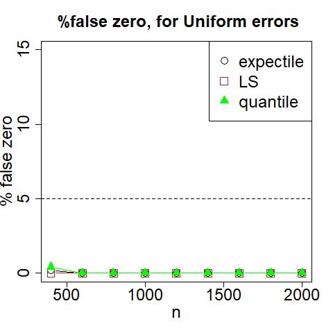
(a) When $\varepsilon\sim{\cal G}(0,1)$, supposition without intercept.	(b) When $\varepsilon\sim{\cal U}[-1,2]-1/6$, supposition without intercept.
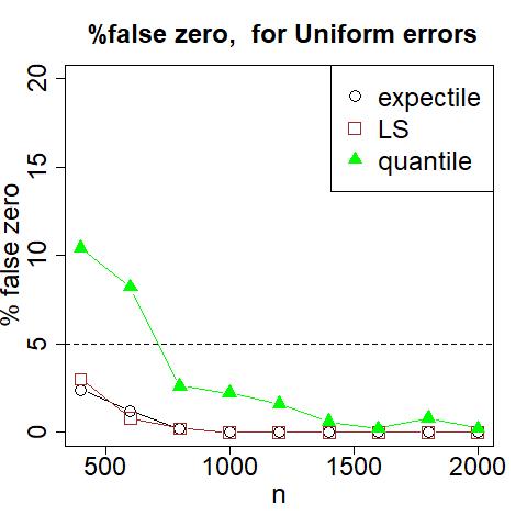
(c) When $\varepsilon\sim{\cal G}(0,1)$, supposition with intercept.	(d) When $\varepsilon\sim{\cal U}[-1,2]-1/6$, supposition with intercept.

Figure 3: Percentage evolution of the false zeros by three censored adaptive LASSO estimation methods, for model without intercept ($\beta^{0}_{0}=0$), when $p=50$ and censoring rate is $25\%$.

(a) Supposition without intercept, $p=50$.	(b) Supposition without intercept, $p=150$.
(c) Supposition with intercept, $p=50$.	(d) Supposition with intercept, $p=150$.

Figure 4: Percentage evolution of the false zeros by three censored adaptive LASSO estimation methods, for model without intercept ($\beta^{0}_{0}=0$), when $\varepsilon\sim{\cal G}(0,1)$ and censoring rate is $10\%$.

(a) $\%$ of true zeros for censoring rate $25\%$.	(b) $\%$ of false zeros for censoring rate $25\%$.
(c) $\%$ of true zeros for censoring rate $10\%$.	(d) $\%$ of false zeros for censoring rate $10\%$.

Figure 5: Percentage evolution of the true and false zeros by three censored adaptive LASSO estimation methods, for model without intercept ($\beta^{0}_{0}=0$), supposition with intercept, when $\varepsilon\sim{\cal G}(0,1)$ and $p=10$.

(a) $\%$ of true zeros, supposition without intercept.	(b) $\%$ of false zeros, supposition without intercept.
(c) $\%$ of true zeros, supposition with intercept.	(d) $\%$ of false zeros, supposition with intercept.

Figure 6: Percentage evolution with respect to the censoring rate of the true and false zeros by three censored adaptive LASSO estimation methods, when $\varepsilon\sim{\cal G}(0,1)$, $n=1000$, $p=50$, model without intercept ($\beta^{0}_{0}=0$).

(a) $\%$ of true zeros.	(b) $\%$ of false zeros.

Figure 7: Percentage evolution of the true and false zeros with respect to L2 beta0 $\equiv\|\textrm{$\mathbf{\beta}^{0}$}\|$ by three censored adaptive LASSO estimation methods, when $\varepsilon\sim{\cal G}(0,1)$, $p=50$, ${\cal A}=\{1,2\}$, model with intercept ($\beta^{0}_{0}=2$) and censoring rate is $25\%$.

(a) Evolution of $L2\equiv\|\widetilde{\textrm{$\mathbf{\beta}$}}_{n}-\textrm{$\mathbf{\beta}^{0}$}\|$.	(b) Evolution of $sd\equiv sd(\widetilde{\textrm{$\mathbf{\beta}$}}_{n}-\textrm{$\mathbf{\beta}^{0}$})$.

Figure 8: Evolution of the accuracy of the parameter estimations by three censored unpenalized estimation methods, when $\varepsilon\sim{\cal G}(0,1)$, $p=2$, $\beta^{0}_{0}=0$, censoring rate $10\%$.

4.4 Numerical study of $\widetilde{\textrm{$\mathbf{\beta}$}}_{n}$

We now study the evolution with $n$ of the accuracy of the censored expectile estimator $\widetilde{\textrm{$\mathbf{\beta}$}}_{n}$ for Gumbel error ${\cal G}(0,1)$, $p=2$: $\beta^{0}_{1}=5\log(n)$, $\beta^{0}_{1}=\log(n)$, $X_{1i}\sim{\cal N}(1,1)$, $X_{2i}\sim{\cal N}(1,5)$, $i=1,\cdots,n$. The considered values for $\mathbf{\beta}^{0}$ allow to investigate the value effect of the parameter norm on the estimator accuracy. Furthermore, for 100 Monte Carlo replications, we compare the censored expectile estimator with the censored least squares and censored quantile estimators by calculating the Euclidean norm $\|\widetilde{\textrm{$\mathbf{\beta}$}}_{n}-\textrm{$\mathbf{\beta}^{0}$}\|$ and the standard deviation of $\widetilde{\textrm{$\mathbf{\beta}$}}_{n}-\textrm{$\mathbf{\beta}^{0}$}$. From the results reported in Table 2 and Figure 8 (symbol $\circ$ for the censored expectile estimator, $\square$ for the censored LS estimator, $\blacktriangle$ for the censored quantile estimator), we deduce that the censored expectile estimators are more accurate than the other two estimators, especially for small values of $n$. The evolution of $\|\widetilde{\textrm{$\mathbf{\beta}$}}_{n}-\textrm{$\mathbf{\beta}^{0}$}\|$ with $n$ in Table 2 also supports the consistency of the estimator $\widetilde{\textrm{$\mathbf{\beta}$}}_{n}$.

$n$	$\|\widetilde{\textrm{$\mathbf{\beta}$}}_{n}-\textrm{$\mathbf{\beta}^{0}$}\|$			$sd(\widetilde{\textrm{$\mathbf{\beta}$}}_{n}-\textrm{$\mathbf{\beta}^{0}$})$
	expectile	LS	quantile	expectile	LS	quantile
10	0.59	0.70	0.68	0.21	0.23	0.23
50	0.25	0.37	0.30	0.09	0.11	0.12
100	0.16	0.29	0.19	0.06	0.08	0.08
200	0.12	0.27	0.14	0.05	0.06	0.05

Table 2: Accuracy results of $\widetilde{\textrm{$\mathbf{\beta}$}}_{n}$ obtained by 100 Monte Carlo replications for three censored unpenalized estimation methods, for model without intercept ($\beta^{0}_{0}=0$), when $\varepsilon\sim{\cal G}(0,1)$, $p=2$, censoring rate $25\%$.

4.5 Conclusion of simulations

The simulation results confirm the consistency and sparsity of the censored adaptive LASSO expectile estimator $\widehat{\textrm{$\mathbf{\beta}$}}_{n}$. The consistency of the censored expectile estimator $\widetilde{\textrm{$\mathbf{\beta}$}}_{n}$ is also shown.
The censored adaptive LASSO expectile estimator produces fewer false zeros and detects the zero coefficients better than the estimators corresponding to the quantile and LS methods. These detections do not depend on the distribution of the model error $\varepsilon$ for each of the three adaptive LASSO methods, but the quantile method produces more false zeros than the expectile and LS methods. On the other hand, for a given censoring rate, when $\varepsilon\sim{\cal G}(0,1)$ and $\lambda_{n}$, $|{\cal A}|$ are fixed, then the percentage of false zeros does not depend on $p$ and $n$. We also obtained that by the censored adaptive LASSO expectile method, the percentage of true zeros and that of false zeros do not evolve with the censoring rate when $|{\cal A}|$, $n$, $p$ are fixed and $\varepsilon\sim{\cal G}(0,1)$. Let us emphasize that the censored adaptive LASSO quantile method detects more and more false zeros as the censoring rate increases.
For the choice of the tuning parameter sequence $(\lambda_{n})_{n\in\mathbb{N}}$ in relation (2) we recommend $\lambda_{n}=o(n^{1/2})$.
We conclude by emphasizing that the censored expectile estimator is more accurate than the censored quantile and censored LS estimators.

5 Applications on real data

In order to support the practical interest of our method, in this section we present the application of the censored adaptive LASSO expectile method on three survival databases. The results are compared to those obtained by the censored adaptive LASSO quantile and LS methods.
Note that for the following three applications, only continuous explanatory variables are considered. These variables are standardized.

5.1 Primary Biliary Cholangitis Data

We will use the non-penalized censored expectile method and the one censored adaptive LASSO expectile on the dataset pbc from the R package survival. The censoring variable ${\cal C}$ is in this case the variable status which indicates the status at the endpoint and which takes three values: 0/1/2 for censored, transplanted, dead, respectively. Initially, there are 418 patients in the study. If the patient received a transplant, then he is also considered as censored. Since the measured variables contain missing values, then the complete database contains $n=276$ observations of which 165 are censored ($\delta_{i}=0$). The failure time $T_{i}$ is the variable time which gives the number of days between registration and the earlier of death. The nine continuous explanatory variables of censored model (3) are: age, albumin, alk, ast, bili, chol, copper, platelet, protime. See the R package survival and its references for a more detailed description of the data.
For these nine variables, the estimation $\widehat{\textrm{$\mathbf{\beta}$}}_{n}$ has seven zero components, more precisely only the variables albumin and protime have non-zero coefficients. Considering censored model (3) only for these two explanatory variables and estimated by the censored expectile method, we obtain the estimations $2.314$ and $2.084$ of the coefficients, respectively.
Note also that the censored adaptive LASSO LS and quantile methods also select the explanatory variables albumin and protime.

5.2 Myeloma

In this subsection we consider two datasets from R packages on myeloma.

5.2.1 Myeloma data of the R package "emplik"

A multiple melanoma study is considered for 65 patients of whom 48 have died and 17 are alive at the end of the study. The survival time $T_{i}$ is measured in months. The seven explanatory continuous variables of model (3) are AGE (age at diagnosis) and expressions of six genes: LOGBUN (log BUN at diagnosis), HGB (hemoglobin at diagnosis), LOGWBC (log WBC at diagnosis), LOGPBM (log percentage of plasma cells in bone marrow), PROTEIN (proteinuria at diagnosis) and SCALC (serum calcium at diagnosis).
The nonzero censored adaptive LASSO expectile estimations are for the coefficients of the variables HGB, AGE, LOGWBC, PROTEIN and SCALC. The coefficient estimations of these variables by the censored expectile method are: -1.3, 2.5, 16.9, 0.7, 2.9, respectively.
Note that by the censored adaptive LASSO LS method the same five variables are selected, results confirmed by hypothesis tests, the residuals of the model being of normal distribution. By the censored adaptive LASSO quantile method only three variables are selected: LOGWBC, PROTEIN and SCALC.

5.2.2 Myeloma data of the R package "survminer"

In this example, we study the survival time (in months) of patients with a multiple melanoma function of gene expression. There are 256 observations in total, but we only analyze 186 because the others have missing data. In the 186 observations, 51 patients have died and 135 are alive. The six continuous explanatory variables are: CCND1, CRIM1, DEPDC1, IRF4, TP53, WHSC1.
By the censored adaptive LASSO expectile method, only the coefficient of IRF4 is non-zero and its estimation by the censored expectile method is 0.49. Note that the same variable is selected by the censored adaptive LASSO LS method. On the other hand, the censored adaptive LASSO quantile method shrinks all coefficients to 0, meaning that no gene expression affects survival time.

6 Proofs

In this section we present the proofs of the results stated in Section 3.

Proof of Theorem 1 (i) Let us consider the random $p$-vector $\widetilde{\mathbf{{u}}}_{n}\equiv n^{1/2}(\widetilde{\textrm{$\mathbf{\beta}$}}_{n}-\textrm{$\mathbf{\beta}^{0}$})$. Thus, in order to prove the convergence rate of $\widetilde{\textrm{$\mathbf{\beta}$}}_{n}$ we consider the parameter $\mathbf{\beta}$ under the form $\textrm{$\mathbf{\beta}$}=\textrm{$\mathbf{\beta}^{0}$}+n^{-1/2}\mathbf{{u}}$, with $\mathbf{{u}}\in\mathbb{R}^{p}$ such that $\|\mathbf{{u}}\|=c<\infty$. Then, let’s study the following random process:

$${\cal R}_{n}(\widehat{G}_{n},\textrm{$\mathbf{\beta}$})\equiv\sum^{n}_{i=1}\frac{\delta_{i}}{\widehat{G}_{n}(Y_{i})}\bigg{(}\rho_{\tau}\big{(}\log(Y_{i})-\mathbf{X}^{\top}_{i}\textrm{$\mathbf{\beta}$}\big{)}-\rho_{\tau}(\varepsilon_{i})\bigg{)}=\sum^{n}_{i=1}\frac{\delta_{i}}{\widehat{G}_{n}(Y_{i})}\bigg{(}\rho_{\tau}\big{(}\varepsilon_{i}-n^{-1/2}\mathbf{X}^{\top}_{i}\mathbf{{u}}\big{)}-\rho_{\tau}(\varepsilon_{i})\bigg{)}.$$

We consider for a survival function $G$ and parameter $\mathbf{\beta}$ the following random process:

$$Q_{n}(G,\textrm{$\mathbf{\beta}$})\equiv\sum^{n}_{i=1}\frac{\delta_{i}}{G(Y_{i})}\rho_{\tau}(\log(Y_{i})-\mathbf{X}_{i}^{\top}\textrm{$\mathbf{\beta}$}).$$

Hence we have ${\cal R}_{n}(\widehat{G}_{n},\textrm{$\mathbf{\beta}$})=Q_{n}(\widehat{G}_{n},\textrm{$\mathbf{\beta}$})-Q_{n}(\widehat{G}_{n},\textrm{$\mathbf{\beta}^{0}$})$, which can be written:

$$Q_{n}(\widehat{G}_{n},\textrm{$\mathbf{\beta}^{0}$}+n^{-1/2}\mathbf{{u}})-Q_{n}(\widehat{G}_{n},\textrm{$\mathbf{\beta}^{0}$}) =\left\{Q_{n}(G_{0},\textrm{$\mathbf{\beta}^{0}$}+n^{-1/2}\mathbf{{u}})-Q_{n}(G_{0},\textrm{$\mathbf{\beta}^{0}$})\right\}$$

$$\quad+\left\{Q_{n}(\widehat{G}_{n},\textrm{$\mathbf{\beta}^{0}$}+n^{-1/2}\mathbf{{u}})-Q_{n}(G_{0},\textrm{$\mathbf{\beta}^{0}$}+n^{-1/2}\mathbf{{u}})\right\}$$

$$\quad-\left\{Q_{n}(\widehat{G}_{n},\textrm{$\mathbf{\beta}^{0}$})-Q_{n}(G_{0},\textrm{$\mathbf{\beta}^{0}$})\right\}$$

$$\equiv{\cal Q}_{1n}+{\cal Q}_{2n}-{\cal Q}_{n}.$$ (4)

By elementary calculus, for $e\in\mathbb{R}$ and $t\rightarrow 0$, we have

$$\rho_{\tau}(e-t)=\rho_{\tau}(e)+g_{\tau}(e)t+h_{\tau}(e)t^{2}/2+o(t^{2}).$$ (5)

For term ${\cal Q}_{1n}$, written as:

$${\cal Q}_{1n}=\sum^{n}_{i=1}\frac{\delta_{i}}{G_{0}(Y_{i})}\big{(}\rho_{\tau}(\varepsilon_{i}-n^{-1/2}\mathbf{X}_{i}^{\top}\mathbf{{u}})-\rho_{\tau}(\varepsilon_{i})\big{)},$$

using the Cauchy-Schwarz inequality together with the fact that $\mathbb{E}_{\cal C}[\delta_{i}]=G_{0}(Y_{i})$, relation (5) and that $\|\mathbf{X}\|$ is bounded by (A5), we get:

$${\cal Q}_{1n}=\sum^{n}_{i=1}\frac{\delta_{i}}{G_{0}(Y_{i})}\bigg{(}g_{\tau}(\varepsilon_{i})\frac{\mathbf{X}_{i}^{\top}\mathbf{{u}}}{\sqrt{n}}+\frac{1}{2}h_{\tau}(\varepsilon_{i})\bigg{(}\frac{\mathbf{X}_{i}^{\top}\mathbf{{u}}}{\sqrt{n}}\bigg{)}^{2}+o_{\mathbb{P}}(n^{-1})\bigg{)}.$$ (6)

On the other hand, using $\mathbb{E}_{\cal C}[\delta_{i}]=G_{0}(Y_{i})$ and $\mathbb{E}_{\varepsilon}[g_{\tau}(\varepsilon_{i})]=0$ of assumption (A7), we have:

$$\mathbb{E}_{\mathbf{X}}\bigg{[}\mathbb{E}_{\varepsilon}\bigg{[}\mathbb{E}_{\cal C}\bigg{[}\frac{\delta_{i}}{G_{0}(Y_{i})}g_{\tau}(\varepsilon_{i})\mathbf{X}_{i}^{\top}\mathbf{{u}}|\varepsilon_{i},\mathbf{X}_{i}\bigg{]}|\mathbf{X}_{i}\bigg{]}\bigg{]}=\mathbb{E}_{\mathbf{X}}\big{[}\mathbb{E}_{\varepsilon}\big{[}g_{\tau}(\varepsilon_{i})\mathbf{X}_{i}^{\top}\mathbf{{u}}|\mathbf{X}_{i}\big{]}\big{]}=0.$$

We proceed in the same way for

$$\mathbb{E}_{\mathbf{X}}\bigg{[}\mathbb{E}_{\varepsilon}\bigg{[}\mathbb{E}_{\cal C}\bigg{[}\bigg{(}\frac{\delta_{i}}{G_{0}(Y_{i})}g_{\tau}(\varepsilon_{i})\frac{\mathbf{X}_{i}^{\top}\mathbf{{u}}}{\sqrt{n}}\bigg{)}^{2}|\varepsilon_{i},\mathbf{X}_{i}\bigg{]}|\mathbf{X}_{i}\bigg{]}\bigg{]} =\mathbb{E}_{\mathbf{X}}\bigg{[}\mathbb{E}_{\varepsilon}\bigg{[}\frac{g^{2}_{\tau}(\varepsilon_{i})}{G_{0}(Y_{i})}\frac{\mathbf{{u}}\mathbf{X}_{i}\mathbf{X}_{i}^{\top}\mathbf{{u}}}{n}|\mathbf{X}_{i}\bigg{]}\bigg{]}$$

$$=\mathbb{E}_{\varepsilon}\big{[}g^{2}_{\tau}(\varepsilon_{i})\big{]}\frac{\mathbf{{u}}^{\top}}{n}\mathbb{E}_{\mathbf{X}}\bigg{[}\frac{\mathbf{X}\mathbf{X}^{\top}}{G_{0}(Y)}\bigg{]}\mathbf{{u}},$$

where we used that $\varepsilon_{i}$ is independent of $\mathbf{X}_{i}$ of assumption (A1). Then, using the Central Limit Theorem (CLT), we get that

$$\sum^{n}_{i=1}\frac{\delta_{i}}{G_{0}(Y_{i})}g_{\tau}(\varepsilon_{i})\frac{\mathbf{X}_{i}^{\top}\mathbf{{u}}}{\sqrt{n}}=\textbf{W}^{\top}_{1}\mathbf{{u}}\big{(}1+o_{\mathbb{P}}(1)\big{)},$$

with the random $p$-vector $\textbf{W}_{1}\sim{\cal N}_{p}(\textrm{$\mathbf{0}$}_{p},\textbf{S}_{1})$.
On the other hand, by the law of large numbers, we have:

$$\frac{1}{n}\sum^{n}_{i=1}\frac{\delta_{i}}{G_{0}(Y_{i})}h_{\tau}(\varepsilon_{i})\mathbf{{u}}^{\top}\mathbf{X}_{i}\mathbf{X}^{\top}_{i}\mathbf{{u}}\overset{\mathbb{P}}{\underset{n\rightarrow\infty}{\longrightarrow}}\mathbb{E}\big{[}h_{\tau}(\varepsilon)\mathbf{{u}}^{\top}\mathbf{X}\mathbf{X}^{\top}\mathbf{{u}}\big{]}=\mathbb{E}_{\varepsilon}\big{[}h_{\tau}(\varepsilon)\big{]}\mathbf{{u}}^{\top}\mathbb{E}_{\mathbf{X}}\big{[}\mathbf{X}\mathbf{X}^{\top}\big{]}\mathbf{{u}}.$$

Taking into account these last relations together with relation (6), then the term ${\cal Q}_{1n}$ becomes:

$${\cal Q}_{1n}=\big{(}\textbf{W}^{\top}_{1}\mathbf{{u}}+\mathbb{E}_{\varepsilon}\big{[}h_{\tau}(\varepsilon)\big{]}\mathbf{{u}}^{\top}\mathbb{E}_{\mathbf{X}}\big{[}\mathbf{X}\mathbf{X}^{\top}\big{]}\mathbf{{u}}\big{)}\big{(}1+o_{\mathbb{P}}(1)\big{)}.$$ (7)

For terms ${\cal Q}_{2n}$ and ${\cal Q}_{3n}$, taking into account assumptions (A4) and (A6), we use the Taylor expansion of $\widehat{G}_{n}(Y_{i})$ with respect to $G_{0}(Y_{i})$:

$$\begin{split}\sqrt{n}\bigg{(}\frac{1}{\widehat{G}_{n}(Y_{i})}-\frac{1}{G_{0}(Y_{i})}\bigg{)}&=-\frac{\sqrt{n}\big{(}\widehat{G}_{n}(Y_{i})-G_{0}(Y_{i})\big{)}}{G^{2}_{0}(Y_{i})}\big{(}1+o_{\mathbb{P}}(1)\big{)}\\ &=\frac{1}{G_{0}(Y_{i})}\frac{1}{\sqrt{n}}\sum^{n}_{j=1}\int^{B}_{0}1\!\!1_{Y_{i}\geq s}\frac{dM_{j}^{\cal C}(s)}{y(s)}\big{(}1+o_{\mathbb{P}}(1)\big{)}.\end{split}$$ (8)

Note that for the martingale representation of $(G_{0}-\widehat{G}_{n})/G_{0}$, the reader can see Fleming and Harrington (1991), page 97 or Chen et al. (2005). Thus

$${\cal Q}_{3n}-{\cal Q}_{2n} =\sum^{n}_{i=1}\delta_{i}\bigg{(}\frac{1}{\widehat{G}_{n}(Y_{i})}-\frac{1}{G_{0}(Y_{i})}\bigg{)}\big{(}\rho_{\tau}(\varepsilon_{i}-n^{1/2}\mathbf{X}^{\top}_{i}\mathbf{{u}})-\rho_{\tau}(\varepsilon_{i})\big{)}$$

$$=\frac{1}{n}\sum^{n}_{i=1}\frac{\delta_{i}}{G_{0}(Y_{i})}\bigg{(}g_{\tau}(\varepsilon_{i})\frac{\mathbf{X}^{\top}_{i}\mathbf{{u}}}{\sqrt{n}}+\frac{h_{\tau}(\varepsilon_{i})}{2}\mathbf{{u}}\frac{\mathbf{X}_{i}\mathbf{X}^{\top}_{i}}{n}\mathbf{{u}}\bigg{)}\sum^{n}_{j=1}\int^{B}_{0}1\!\!1_{Y_{i}\geq s}\frac{dM^{\cal C}_{j}(s)}{y(s)}\big{(}1+o_{\mathbb{P}}(1)\big{)}$$

$$=\frac{1}{n}\sum^{n}_{i=1}\frac{\delta_{i}}{G_{0}(Y_{i})}g_{\tau}(\varepsilon_{i})\frac{\mathbf{X}^{\top}_{i}\mathbf{{u}}}{\sqrt{n}}\sum^{n}_{j=1}\int^{B}_{0}1\!\!1_{Y_{i}\geq s}\frac{dM^{\cal C}_{j}(s)}{y(s)}\big{(}1+o_{\mathbb{P}}(1)\big{)}.$$

For the second equality we used relation (8), together with the fact that $\|\mathbf{X}\|<\infty$ of assumption (A5) and with relation (5) for $t=n^{-1/2}\mathbf{X}_{i}^{\top}\mathbf{{u}}$. Thus, by the law of large numbers, we have:

$${\cal Q}_{3n}-{\cal Q}_{2n}=\frac{\mathbf{{u}}^{\top}}{\sqrt{n}}\sum^{n}_{j=1}\int^{B}_{0}\frac{\textrm{$\mathbf{\kappa}$}(s)}{y(s)}dM^{\cal C}_{j}(s)\big{(}1+o_{\mathbb{P}}(1)\big{)}.$$ (9)

By the martingale CLT we have:

$$\frac{\mathbf{{u}}^{\top}}{\sqrt{n}}\sum^{n}_{j=1}\int^{B}_{0}\frac{\textrm{$\mathbf{\kappa}$}(s)}{y(s)}dM^{\cal C}_{j}(s)\overset{\cal L}{\underset{n\rightarrow\infty}{\longrightarrow}}\mathbf{{u}}^{\top}\textbf{W}_{2},$$ (10)

with the random $p$-vector $\textbf{W}_{2}\sim{\cal N}_{p}(\textrm{$\mathbf{0}$}_{p},\textbf{S}_{2})$.
Hence, we have shown, by relations (6), (7), (9) and (10), that:

$$Q_{n}(\widehat{G}_{n},\textrm{$\mathbf{\beta}^{0}$}+n^{-1/2}\mathbf{{u}})-Q_{n}(\widehat{G}_{n},\textrm{$\mathbf{\beta}^{0}$})=\bigg{(}\mathbf{{u}}^{\top}\textbf{W}_{1}+\frac{\mathbb{E}_{\varepsilon}\big{[}h_{\tau}(\varepsilon)\big{]}}{2}\mathbf{{u}}^{\top}\mathbb{E}_{\mathbf{X}}[\mathbf{X}\mathbf{X}^{\top}]\mathbf{{u}}+\mathbf{{u}}^{\top}\textbf{W}_{2}\bigg{)}\big{(}1+o_{\mathbb{P}}(1)\big{)},$$

where, for $c=\|\mathbf{{u}}\|$ large enough, we have that $\mathbb{E}_{\varepsilon}\big{[}h_{\tau}(\varepsilon)\big{]}\mathbf{{u}}^{\top}\mathbb{E}_{\mathbf{X}}[\mathbf{X}\mathbf{X}^{\top}]\mathbf{{u}}$ dominates $\mathbf{{u}}^{\top}(\textbf{W}_{1}+\textbf{W}_{2})$. This implies that for all $\epsilon>0$, for large $n$, we have:

$$\mathbb{P}\bigg{[}\inf_{\|\mathbf{{u}}\|=c}\big{[}Q_{n}(\widehat{G}_{n},\textrm{$\mathbf{\beta}^{0}$}+n^{-1/2}\mathbf{{u}})-Q_{n}(\widehat{G}_{n},\textrm{$\mathbf{\beta}^{0}$})\big{]}>0\bigg{]}\geq 1-\epsilon,$$

which involves that $\widetilde{\textrm{$\mathbf{\beta}$}}_{n}-\textrm{$\mathbf{\beta}^{0}$}=O_{\mathbb{P}}(n^{-1/2})$ and statement (i) is proved.
(ii) In view of statement (i), we have that the minimizer in $\mathbf{{u}}$ of $Q_{n}(\widehat{G}_{n},\textrm{$\mathbf{\beta}^{0}$}+n^{-1/2}\mathbf{{u}})$ is the solution of the following system of $p$ equations:

$$\textbf{W}_{1}+\mathbb{E}_{\varepsilon}\big{[}h_{\tau}(\varepsilon)\big{]}\mathbb{E}_{\mathbf{X}}[\mathbf{X}\mathbf{X}^{\top}]\mathbf{{u}}+\textbf{W}_{2}=\textrm{$\mathbf{0}$}_{p}.$$

The solution of this system is $\mathbf{{u}}=-(\textbf{W}_{1}+\textbf{W}_{2})\mathbb{E}^{-1}_{\varepsilon}\big{[}h_{\tau}(\varepsilon)\big{]}\mathbb{E}_{\mathbf{X}}[\mathbf{X}\mathbf{X}^{\top}]^{-1}$. On the other hand, since $\textbf{W}_{1}+\textbf{W}_{2}\sim{\cal N}_{p}(\textrm{$\mathbf{0}$}_{p},\textbf{S}_{1}+\textbf{S}_{2})$, then $\mathbf{{u}}\sim{\cal N}_{p}\big{(}\textrm{$\mathbf{0}$}_{p},\textbf{S}^{-1}_{3}(\textbf{S}_{1}+\textbf{S}_{2})\textbf{S}^{-1}_{3}\big{)}$ and statement (ii) is proved. $\blacksquare$

Proof of Theorem 2. For a survival function $G$ and a parameter $p$-vector $\mathbf{\beta}$, let us consider the following random process:

$${\cal T}_{n}(G,\textrm{$\mathbf{\beta}$})\equiv Q_{n}(G,\textrm{$\mathbf{\beta}$})-Q_{n}(G,\textrm{$\mathbf{\beta}^{0}$})+\lambda_{n}\sum^{p}_{j=1}\widehat{\omega}_{n,j}\big{(}|\beta_{j}|-|\beta^{0}_{j}|\big{)}.$$

We can write

$${\cal T}_{n}(\widehat{G}_{n},\textrm{$\mathbf{\beta}$})={\cal R}_{n}(\widehat{G}_{n},\textrm{$\mathbf{\beta}$})+\lambda_{n}\sum^{p}_{j=1}\widehat{\omega}_{n,j}\big{(}|\beta_{j}|-|\beta^{0}_{j}|\big{)},$$ (11)

with ${\cal R}_{n}(\widehat{G}_{n},\textrm{$\mathbf{\beta}$})$ defined in the proof of Theorem 1. Consider the $p$-vector $\mathbf{{u}}=(u_{1},\cdots,u_{p})$. For the second term of the right-hand side of relation (11) we have with probability one that

$$\sum^{p}_{j=1}\widehat{\omega}_{n,j}\big{(}|\beta^{0}_{j}+n^{-1/2}u_{j}|-|\beta^{0}_{j}|\big{)} =\sum^{q}_{j=1}\widehat{\omega}_{n,j}\big{(}|\beta^{0}_{j}+n^{-1/2}u_{j}|-|\beta^{0}_{j}|\big{)}+\sum^{p}_{j=q+1}\widehat{\omega}_{n,j}n^{-1/2}|u_{j}|$$

$$\geq\sum^{q}_{j=1}\widehat{\omega}_{n,j}\big{(}|\beta^{0}_{j}+n^{-1/2}u_{j}|-|\beta^{0}_{j}|\big{)}.$$

On the other hand, using Theorem 1 we have that $\widehat{\omega}_{n,j}=O_{\mathbb{P}}(1)$ for all $j\in\{1,\cdots,q\}$, which implies with probability converging to one that:

$$\sum^{p}_{j=1}\widehat{\omega}_{n,j}\big{(}|\beta^{0}_{j}+n^{-1/2}u_{j}|-|\beta^{0}_{j}|\big{)}\geq-c\sum^{q}_{j=1}n^{-1/2}|u_{j}|.$$

Then, since $n^{-1/2}\lambda_{n}=O_{\mathbb{P}}(1)$, we have:

$$\lambda_{n}\sum^{p}_{j=1}\widehat{\omega}_{n,j}\big{(}|\beta^{0}_{j}+n^{-1/2}u_{j}|-|\beta^{0}_{j}|\big{)}\geq-O_{\mathbb{P}}(\|\mathbf{{u}}\|).$$ (12)

On the other hand, by the proof of Theorem 1, for $\|\mathbf{{u}}\|$ large enough, we have for the first term of the right-hand side of relation (11):

$$Q_{n}(\widehat{G}_{n},\textrm{$\mathbf{\beta}^{0}$}+n^{-1/2}\mathbf{{u}})-Q_{n}(\widehat{G}_{n},\textrm{$\mathbf{\beta}^{0}$})=\frac{\mathbb{E}_{\varepsilon}[h_{\tau}(\varepsilon)]}{2}\mathbf{{u}}^{\top}\mathbb{E}_{\mathbf{X}}[\mathbf{X}\mathbf{X}^{\top}]\mathbf{{u}}\big{(}1+o_{\mathbb{P}}(1)\big{)}.$$ (13)

From relations (11), (12) and (13) we obtain

$${\cal T}_{n}\big{(}\widehat{G}_{n},\textrm{$\mathbf{\beta}^{0}$}+n^{-1/2}\mathbf{{u}}\big{)}=O_{\mathbb{P}}(\|\mathbf{{u}}\|^{2}),$$

for $\|\mathbf{{u}}\|$ large enough. Thus, $\widehat{\textrm{$\mathbf{\beta}$}}_{n}-\textrm{$\mathbf{\beta}^{0}$}=O_{\mathbb{P}}(n^{-1/2})$, which implies the theorem. $\blacksquare$

Proof of Theorem 3 (i) Taking into account the convergence rate of $\widehat{\textrm{$\mathbf{\beta}$}}_{n}$ towards $\mathbf{\beta}^{0}$ obtained by Theorem 2, let us consider the following sets of parameters ${\cal V}(\textrm{$\mathbf{\beta}^{0}$})\equiv\big{\{}\textrm{$\mathbf{\beta}$};\|\textrm{$\mathbf{\beta}$}-\textrm{$\mathbf{\beta}^{0}$}\|\leq cn^{-1/2}\big{\}}$ and ${\cal W}_{n}\equiv\big{\{}\textrm{$\mathbf{\beta}$}\in{\cal V}(\textrm{$\mathbf{\beta}^{0}$});\|\textrm{$\mathbf{\beta}$}_{{\cal A}^{c}}\|>0\big{\}}$. Theorem 2 implies that $\widehat{\textrm{$\mathbf{\beta}$}}_{n}$ belongs to ${\cal V}(\textrm{$\mathbf{\beta}^{0}$})$ with probability converging to 1 when $n\rightarrow\infty$. In order to prove the theorem, we will first show that $\mathbb{P}[\widehat{\textrm{$\mathbf{\beta}$}}_{n}\in{\cal W}_{n}]{\underset{n\rightarrow\infty}{\longrightarrow}}0$.
Recall that the true parameter is $\textrm{$\mathbf{\beta}^{0}$}=\big{(}\textrm{$\mathbf{\beta}$}^{0}_{\cal A},\textrm{$\mathbf{0}$}_{|{\cal A}^{c}|}\big{)}$. Then, in order to show the sparsity of $\widehat{\textrm{$\mathbf{\beta}$}}_{n}$, we consider two parameters $\textrm{$\mathbf{\beta}$}^{(1)}\equiv\big{(}\textrm{$\mathbf{\beta}$}^{(1)}_{\cal A},\textrm{$\mathbf{\beta}$}^{(1)}_{{\cal A}^{c}}\big{)}\in{\cal V}(\textrm{$\mathbf{\beta}^{0}$})\setminus{\cal W}_{n}$ , $\textrm{$\mathbf{\beta}$}^{(2)}\equiv\big{(}\textrm{$\mathbf{\beta}$}^{(2)}_{\cal A},\textrm{$\mathbf{\beta}$}^{(2)}_{{\cal A}^{c}}\big{)}\in{\cal W}_{n}$, with $\textrm{$\mathbf{\beta}$}^{(1)}_{{\cal A}^{c}}=\textrm{$\mathbf{0}$}_{|{\cal A}^{c}|}$ and $\textrm{$\mathbf{\beta}$}^{(2)}_{\cal A}=\textrm{$\mathbf{\beta}$}^{(1)}_{\cal A}$. Let’s calculate

$${\cal T}_{n}(\widehat{G}_{n},\textrm{$\mathbf{\beta}$}^{(2)})-{\cal T}_{n}(\widehat{G}_{n},\textrm{$\mathbf{\beta}$}^{(1)})=Q_{n}(\widehat{G}_{n},\textrm{$\mathbf{\beta}$}^{(2)})-Q_{n}(\widehat{G}_{n},\textrm{$\mathbf{\beta}$}^{(1)})+\lambda_{n}\sum^{p}_{j=1}\widehat{\omega}_{n,j}\big{(}|\beta^{(2)}_{j}|-|\beta^{(1)}_{j}|\big{)}.$$ (14)

Then, for the first term of the right-hand side of relation (14), taking in relation (5), $e=\varepsilon_{i}$ and $t=\mathbf{X}^{\top}_{i}(\textrm{$\mathbf{\beta}$}^{(2)}-\textrm{$\mathbf{\beta}^{0}$})$ or $t=\mathbf{X}^{\top}_{i}(\textrm{$\mathbf{\beta}$}^{(1)}-\textrm{$\mathbf{\beta}^{0}$})$ and using assumption (A5), we obtain:

$$Q_{n}(\widehat{G}_{n},\textrm{$\mathbf{\beta}$}^{(2)})-Q_{n}(\widehat{G}_{n},\textrm{$\mathbf{\beta}$}^{(1)})=\sum^{n}_{i=1}\frac{\delta_{i}}{\widehat{G}_{n}(Y_{i})}\bigg{(}\rho_{\tau}\big{(}\log(Y_{i})-\mathbf{X}_{i}^{\top}\textrm{$\mathbf{\beta}$}^{(2)}\big{)}-\rho_{\tau}\big{(}\log(Y_{i})-\mathbf{X}_{i}^{\top}\textrm{$\mathbf{\beta}$}^{(1)}\big{)}\bigg{)}$$

$$=\sum^{n}_{i=1}\frac{\delta_{i}}{\widehat{G}_{n}(Y_{i})}\bigg{\{}\bigg{(}g_{\tau}(\varepsilon_{i})\mathbf{X}^{\top}_{i}\big{(}\textrm{$\mathbf{\beta}$}^{(2)}_{{\cal A}}-\textrm{$\mathbf{\beta}^{0}$}_{\cal A},\textrm{$\mathbf{\beta}$}^{(2)}_{{\cal A}^{c}}\big{)}+\frac{h_{\tau}(\varepsilon_{i})}{2}\big{(}\mathbf{X}^{\top}_{i}\big{(}\textrm{$\mathbf{\beta}$}^{(2)}_{{\cal A}}-\textrm{$\mathbf{\beta}^{0}$}_{\cal A},\textrm{$\mathbf{\beta}$}^{(2)}_{{\cal A}^{c}}\big{)}\big{)}^{2}$$

$$\qquad\qquad+o_{\mathbb{P}}\big{(}\mathbf{X}^{\top}_{i}\big{(}\textrm{$\mathbf{\beta}$}^{(2)}_{{\cal A}}-\textrm{$\mathbf{\beta}^{0}$}_{\cal A},\textrm{$\mathbf{\beta}$}^{(2)}_{{\cal A}^{c}}\big{)}\big{)}^{2}\bigg{)}$$

$$-\bigg{(}g_{\tau}(\varepsilon_{i})\mathbf{X}^{\top}_{{\cal A},i}\big{(}\textrm{$\mathbf{\beta}$}^{(2)}-\textrm{$\mathbf{\beta}^{0}$}\big{)}_{\cal A}+\frac{h_{\tau}(\varepsilon_{i})}{2}\big{(}\mathbf{X}^{\top}_{i,{\cal A}}\big{(}\textrm{$\mathbf{\beta}$}^{(2)}-\textrm{$\mathbf{\beta}^{0}$}\big{)}_{\cal A}\big{)}^{2}+o_{\mathbb{P}}\big{(}\mathbf{X}^{\top}_{{\cal A},i}\big{(}\textrm{$\mathbf{\beta}$}^{(2)}-\textrm{$\mathbf{\beta}^{0}$}\big{)}_{\cal A}\big{)}^{2}\bigg{)}\bigg{\}}$$

$$=\sum^{n}_{i=1}\frac{\delta_{i}}{G_{0}(Y_{i})}\bigg{\{}\bigg{(}g_{\tau}(\varepsilon_{i})\mathbf{X}^{\top}_{i}\big{(}\textrm{$\mathbf{\beta}$}^{(2)}_{{\cal A}}-\textrm{$\mathbf{\beta}^{0}$}_{\cal A},\textrm{$\mathbf{\beta}$}^{(2)}_{{\cal A}^{c}}\big{)}+\frac{h_{\tau}(\varepsilon_{i})}{2}\big{(}\mathbf{X}^{\top}_{i}\big{(}\textrm{$\mathbf{\beta}$}^{(2)}_{{\cal A}}-\textrm{$\mathbf{\beta}^{0}$}_{\cal A},\textrm{$\mathbf{\beta}$}^{(2)}_{{\cal A}^{c}}\big{)}\big{)}^{2}$$

$$\qquad\qquad+o_{\mathbb{P}}\big{(}\mathbf{X}^{\top}_{i}\big{(}\textrm{$\mathbf{\beta}$}^{(2)}_{{\cal A}}-\textrm{$\mathbf{\beta}^{0}$}_{\cal A},\textrm{$\mathbf{\beta}$}^{(2)}_{{\cal A}^{c}}\big{)}\big{)}^{2}\bigg{)}$$

$$-\bigg{(}g_{\tau}(\varepsilon_{i})\mathbf{X}^{\top}_{{\cal A},i}\big{(}\textrm{$\mathbf{\beta}$}^{(2)}-\textrm{$\mathbf{\beta}^{0}$}\big{)}_{\cal A}+\frac{h_{\tau}(\varepsilon_{i})}{2}\big{(}\mathbf{X}^{\top}_{{\cal A},i}\big{(}\textrm{$\mathbf{\beta}$}^{(2)}-\textrm{$\mathbf{\beta}^{0}$}\big{)}_{\cal A}\big{)}^{2}+o_{\mathbb{P}}\big{(}\mathbf{X}^{\top}_{{\cal A},i}\big{(}\textrm{$\mathbf{\beta}$}^{(2)}-\textrm{$\mathbf{\beta}^{0}$}\big{)}_{\cal A}\big{)}^{2}\bigg{)}\bigg{\}}$$

$$+\sum^{n}_{i=1}\delta_{i}\bigg{(}\frac{1}{\widehat{G}_{n}(Y_{i})}-\frac{1}{G_{0}(Y_{i})}\bigg{)}\bigg{\{}\bigg{(}g_{\tau}(\varepsilon_{i})\mathbf{X}^{\top}_{i}\big{(}\textrm{$\mathbf{\beta}$}^{(2)}_{{\cal A}}-\textrm{$\mathbf{\beta}^{0}$}_{\cal A},\textrm{$\mathbf{\beta}$}^{(2)}_{{\cal A}^{c}}\big{)}+\frac{h_{\tau}(\varepsilon_{i})}{2}\big{(}\mathbf{X}^{\top}_{i}\big{(}\textrm{$\mathbf{\beta}$}^{(2)}_{{\cal A}}-\textrm{$\mathbf{\beta}^{0}$}_{\cal A},\textrm{$\mathbf{\beta}$}^{(2)}_{{\cal A}^{c}}\big{)}\big{)}^{2}$$

$$\qquad\qquad+o_{\mathbb{P}}\big{(}\mathbf{X}^{\top}_{i}\big{(}\textrm{$\mathbf{\beta}$}^{(2)}_{{\cal A}}-\textrm{$\mathbf{\beta}^{0}$}_{\cal A},\textrm{$\mathbf{\beta}$}^{(2)}_{{\cal A}^{c}}\big{)}\big{)}^{2}\bigg{)}$$

$$-\bigg{(}g_{\tau}(\varepsilon_{i})\mathbf{X}^{\top}_{{\cal A},i}\big{(}\textrm{$\mathbf{\beta}$}^{(2)}-\textrm{$\mathbf{\beta}^{0}$}\big{)}_{\cal A}+\frac{h_{\tau}(\varepsilon_{i})}{2}\big{(}\mathbf{X}^{\top}_{{\cal A},i}\big{(}\textrm{$\mathbf{\beta}$}^{(2)}-\textrm{$\mathbf{\beta}^{0}$}\big{)}_{\cal A}\big{)}^{2}+o_{\mathbb{P}}\big{(}\mathbf{X}^{\top}_{{\cal A},i}\big{(}\textrm{$\mathbf{\beta}$}^{(2)}-\textrm{$\mathbf{\beta}^{0}$}\big{)}_{\cal A}\big{)}^{2}\bigg{)}\bigg{\}}$$

Taking into account relation (8), this is equal to

$$=\sum^{n}_{i=1}\frac{\delta_{i}}{G_{0}(Y_{i})}\bigg{\{}\bigg{(}g_{\tau}(\varepsilon_{i})\mathbf{X}^{\top}_{{\cal A}^{c},i}\textrm{$\mathbf{\beta}$}^{(2)}_{{\cal A}^{c}}+\frac{h_{\tau}(\varepsilon_{i})}{2}\big{(}\mathbf{X}^{\top}_{i}\big{(}\textrm{$\mathbf{\beta}$}^{(2)}_{{\cal A}}-\textrm{$\mathbf{\beta}^{0}$}_{\cal A},\textrm{$\mathbf{\beta}$}^{(2)}_{{\cal A}^{c}}\big{)}\big{)}^{2}+o_{\mathbb{P}}\big{(}\mathbf{X}^{\top}_{i}\big{(}\textrm{$\mathbf{\beta}$}^{(2)}_{{\cal A}}-\textrm{$\mathbf{\beta}^{0}$}_{\cal A},\textrm{$\mathbf{\beta}$}^{(2)}_{{\cal A}^{c}}\big{)}\big{)}\bigg{)}$$

$$\qquad-\bigg{(}\frac{h_{\tau}(\varepsilon_{i})}{2}\big{(}\mathbf{X}^{\top}_{{\cal A},i}\big{(}\textrm{$\mathbf{\beta}$}^{(2)}-\textrm{$\mathbf{\beta}^{0}$}\big{)}_{\cal A}\big{)}^{2}+o_{\mathbb{P}}\big{(}\mathbf{X}^{\top}_{{\cal A},i}\big{(}\textrm{$\mathbf{\beta}$}^{(2)}-\textrm{$\mathbf{\beta}^{0}$}\big{)}_{\cal A}\big{)}\bigg{)}\bigg{\}}$$

$$+\sum^{n}_{i=1}\frac{\delta_{i}}{G_{0}(Y_{i})}\bigg{\{}\bigg{(}g_{\tau}(\varepsilon_{i})\mathbf{X}^{\top}_{i,{\cal A}^{c}}\textrm{$\mathbf{\beta}$}^{(2)}_{{\cal A}^{c}}+\frac{h_{\tau}(\varepsilon_{i})}{2}\big{(}\mathbf{X}^{\top}_{i}\big{(}\textrm{$\mathbf{\beta}$}^{(2)}_{{\cal A}}-\textrm{$\mathbf{\beta}^{0}$}_{\cal A},\textrm{$\mathbf{\beta}$}^{(2)}_{{\cal A}^{c}}\big{)}\big{)}^{2}+o_{\mathbb{P}}\big{(}\mathbf{X}^{\top}_{i}\big{(}\textrm{$\mathbf{\beta}$}^{(2)}_{{\cal A}}-\textrm{$\mathbf{\beta}^{0}$}_{\cal A},\textrm{$\mathbf{\beta}$}^{(2)}_{{\cal A}^{c}}\big{)}\big{)}^{2}\bigg{)}$$

$$-\bigg{(}\frac{h_{\tau}(\varepsilon_{i})}{2}\big{(}\mathbf{X}^{\top}_{{\cal A},i}\big{(}\textrm{$\mathbf{\beta}$}^{(2)}-\textrm{$\mathbf{\beta}^{0}$}\big{)}_{\cal A}\big{)}^{2}+o_{\mathbb{P}}\big{(}\mathbf{X}^{\top}_{{\cal A},i}\big{(}\textrm{$\mathbf{\beta}$}^{(2)}-\textrm{$\mathbf{\beta}^{0}$}\big{)}_{\cal A}\big{)}\bigg{)}\bigg{\}}\frac{1}{n}\sum^{n}_{j=1}\int^{B}_{0}1\!\!1_{Y_{i}\geq s}\frac{dM_{j}^{\cal C}(s)}{y(s)}\big{(}1+o_{\mathbb{P}}(1)\big{)}$$

$$\equiv\mathbb{S}_{1}+\mathbb{S}_{2}\equiv(S_{11}-S_{12})+(S_{21}-S_{22}).$$

We analyze in the following each terms $S_{11}$, $S_{12}$, $S_{21}$ and $S_{22}$. Let’s start with $S_{11}$. Since, by the CLT

$$n^{-1/2}\sum^{n}_{i=1}\frac{\delta_{i}}{G_{0}(Y_{i})}g_{\tau}(\varepsilon_{i})\mathbf{X}_{{\cal A}^{c},i}\overset{\cal L}{\underset{n\rightarrow\infty}{\longrightarrow}}{\cal N}_{|{\cal A}^{c}|}(\textrm{$\mathbf{0}$}_{q},\textbf{S}_{1,{\cal A}^{c}}),$$

then, we obtain

$$\sum^{n}_{i=1}\frac{\delta_{i}}{G_{0}(Y_{i})}g_{\tau}(\varepsilon_{i})\mathbf{X}^{\top}_{{\cal A}^{c},i}\textrm{$\mathbf{\beta}$}^{(2)}_{{\cal A}^{c}}=O_{\mathbb{P}}(1).$$ (15)

On the other hand, taking into account assumption (A5), we get:

$$\frac{1}{n}\sum^{n}_{i=1}\frac{\delta_{i}}{G_{0}(Y_{i})}\frac{h_{\tau}(\varepsilon_{i})}{2}\big{(}\mathbf{X}^{\top}_{i}\big{(}\textrm{$\mathbf{\beta}$}^{(2)}_{{\cal A}}-\textrm{$\mathbf{\beta}^{0}$}_{\cal A},\textrm{$\mathbf{\beta}$}^{(2)}_{{\cal A}^{c}}\big{)}\big{)}^{2}=O_{\mathbb{P}}\big{(}\|\textrm{$\mathbf{\beta}$}^{(2)}-\textrm{$\mathbf{\beta}^{0}$}\|^{2}\big{)}=O_{\mathbb{P}}(n^{-1}).$$ (16)

Relations (15) and (16) imply that $S_{11}=O_{\mathbb{P}}(1)$. We show similarly that $S_{12}=O_{\mathbb{P}}(1)$ and then we obtain $\mathbb{S}_{1}=O_{\mathbb{P}}(1)$.
For term $\mathbb{S}_{2}$, we first study $S_{21}$. Taking into account the definition of the random vector $\textrm{$\mathbf{\kappa}$}(s)$, we obtain:

$$\frac{1}{n}\sum^{n}_{i=1}\frac{\delta_{i}}{G_{0}(Y_{i})}g_{\tau}(\varepsilon_{i})\mathbf{X}^{\top}_{{\cal A}^{c},i}1\!\!1_{Y_{i}\geq s}=O_{\mathbb{P}}(1)\overset{\mathbb{P}}{\underset{n\rightarrow\infty}{\longrightarrow}}\textrm{$\mathbf{\kappa}$}_{{\cal A}^{c}}(s).$$ (17)

By the martingale CLT we have

$$\frac{1}{\sqrt{n}}\sum^{n}_{j=1}\int^{B}_{0}\frac{\textrm{$\mathbf{\kappa}$}_{{\cal A}^{c}}(s)}{y(s)}dM^{\cal C}_{j}(s)\overset{\cal L}{\underset{n\rightarrow\infty}{\longrightarrow}}\textbf{W}_{2,{\cal A}^{c}}\sim{\cal N}_{|{\cal A}^{c}|}\big{(}\textrm{$\mathbf{0}$}_{|{\cal A}^{c}|},...\big{)},$$

which implies, using Slutsky’s Lemma, that,

$$n^{-1}\sum^{n}_{j=1}\int^{B}_{0}\frac{\textrm{$\mathbf{\kappa}$}_{{\cal A}^{c}}(s)}{y(s)}dM^{\cal C}_{j}(s)\textrm{$\mathbf{\beta}$}^{(2)}_{{\cal A}^{c}}=o_{\mathbb{P}}(1).$$

Thus, using also relation (17), we obtain:

$$\sum^{n}_{i=1}\frac{\delta_{i}}{G_{0}(Y_{i})}g_{\tau}(\varepsilon_{i})\mathbf{X}^{\top}_{{\cal A}^{c},i}\textrm{$\mathbf{\beta}$}^{(2)}_{{\cal A}^{c}}\frac{1}{n}\sum^{n}_{j=1}\int^{B}_{0}1\!\!1_{Y_{i}\geq s}\frac{dM_{j}^{\cal C}(s)}{y(s)}=O_{\mathbb{P}}(1).$$

Taking into account relation (16) we obtain that $S_{21}=O_{\mathbb{P}}(1)$. We show similarly that $S_{22}=O_{\mathbb{P}}(1)$. We have then $\mathbb{S}_{2}=O_{\mathbb{P}}(1)$.
In conclusion, we showed that

$$Q_{n}(\widehat{G}_{n},\textrm{$\mathbf{\beta}$}^{(2)})-Q_{n}(\widehat{G}_{n},\textrm{$\mathbf{\beta}$}^{(1)})=O_{\mathbb{P}}(1).$$ (18)

On the other hand, taking into account Theorem 1(i) and the assumption $n^{(\gamma-1)/2}\lambda_{n}{\underset{n\rightarrow\infty}{\longrightarrow}}\infty$, we obtain:

$$\begin{split}\lambda_{n}\sum^{p}_{j=1}\widehat{\omega}_{n,j}\big{(}|\beta^{(2)}_{j}|-|\beta^{(1)}_{j}|\big{)}&=\lambda_{n}\sum^{p}_{j=q+1}\widehat{\omega}_{n,j}|\beta^{(2)}_{j}|\\ &\geq O_{\mathbb{P}}\big{(}\lambda_{n}n^{\gamma/2}n^{-1/2}\big{)}=O_{\mathbb{P}}(\lambda_{n}n^{(\gamma-1)/2}){\underset{n\rightarrow\infty}{\longrightarrow}}\infty.\end{split}$$ (19)

Relations (18) and (19) imply that the penalty dominates in ${\cal T}_{n}(\widehat{G}_{n},\textrm{$\mathbf{\beta}$}^{(2)})-{\cal T}_{n}(\widehat{G}_{n},\textrm{$\mathbf{\beta}$}^{(1)})$ of relation (14), penalty which is the order $\lambda_{n}n^{(\gamma-1)/2}{\underset{n\rightarrow\infty}{\longrightarrow}}\infty$. On the other hand, by a calculation similar to that of relation (18), we obtain that: ${\cal T}_{n}(\widehat{G}_{n},\textrm{$\mathbf{\beta}$}^{0})-{\cal T}_{n}(\widehat{G}_{n},\textrm{$\mathbf{\beta}$}^{(1)})=Q_{n}(\widehat{G}_{n},\textrm{$\mathbf{\beta}$}^{0})-Q_{n}(\widehat{G}_{n},\textrm{$\mathbf{\beta}$}^{(1)})=O_{\mathbb{P}}(1)$. These imply that $\textrm{$\mathbf{\beta}$}^{(2)}$ cannot be a minimum point of ${\cal T}_{n}(\widehat{G}_{n},\textrm{$\mathbf{\beta}$})$. Thus, we have that $\mathbb{P}[\widehat{\textrm{$\mathbf{\beta}$}}_{n}\in{\cal W}_{n}]{\underset{n\rightarrow\infty}{\longrightarrow}}0$ which implies $\mathbb{P}[\widehat{\textrm{$\mathbf{\beta}$}}_{n}\in{\cal A}^{c}\cap\widehat{\cal A}_{n}]{\underset{n\rightarrow\infty}{\longrightarrow}}0$, from where $\mathbb{P}[\widehat{\cal A}_{n}\subseteq{\cal A}]{\underset{n\rightarrow\infty}{\longrightarrow}}1$. Since $\widehat{\textrm{$\mathbf{\beta}$}}_{n,{\cal A}}$ is consistent, then $\widehat{\textrm{$\mathbf{\beta}$}}_{n,{\cal A}}\overset{\mathbb{P}}{\underset{n\rightarrow\infty}{\longrightarrow}}\textrm{$\mathbf{\beta}$}^{0}_{\cal A}\neq\textrm{$\mathbf{0}$}_{|{\cal A}|}$, which implies $\mathbb{P}[{\cal A}\subseteq\widehat{\cal A}_{n}]{\underset{n\rightarrow\infty}{\longrightarrow}}1$. We have shown that $\mathbb{P}[{\cal A}=\widehat{\cal A}_{n}]{\underset{n\rightarrow\infty}{\longrightarrow}}1$, that is statement (i).
(ii) In virtue of statement (i), we consider the parameter $\textrm{$\mathbf{\beta}$}=(\textrm{$\mathbf{\beta}$}_{\cal A},\textrm{$\mathbf{\beta}$}_{{\cal A}^{c}})$ such that $\textrm{$\mathbf{\beta}$}_{\cal A}=\textrm{$\mathbf{\beta}$}^{0}_{\cal A}+n^{-1/2}\mathbf{{u}}_{\cal A}$ and $\textrm{$\mathbf{\beta}$}_{{\cal A}^{c}}=\textrm{$\mathbf{0}$}_{|{\cal A}^{c}|}$, $\mathbf{{u}}=(\mathbf{{u}}_{\cal A},\textrm{$\mathbf{0}$}_{|{\cal A}^{c}|})$, with $\|\mathbf{{u}}_{\cal A}\|\leq c\leq\infty$. Then, combining relation (5) with assumption (A5), we get:

$${\cal T}_{n}\big{(}\widehat{G}_{n},n^{-1/2}(\mathbf{{u}}_{\cal A},\textrm{$\mathbf{0}$}_{|{\cal A}^{c}|})\big{)}=Q_{n}\big{(}\widehat{G}_{n},\textrm{$\mathbf{\beta}^{0}$}+n^{-1/2}\mathbf{{u}}\big{)}-Q_{n}(\widehat{G}_{n},\textrm{$\mathbf{\beta}^{0}$})+\lambda_{n}\sum^{q}_{j=1}\big{(}|\beta^{0}_{j}+n^{-1/2}u_{j}|-|\beta^{0}_{j}|\big{)}$$

$$=\sum^{n}_{i=1}\frac{\delta_{i}}{\widehat{G}_{n}(Y_{i})}\big{(}\rho_{\tau}(\varepsilon_{i}-n^{-1/2}\mathbf{X}^{\top}_{{\cal A},i}\mathbf{{u}}_{\cal A})-\rho_{\tau}(\varepsilon_{i})\big{)}+\lambda_{n}\sum^{q}_{j=1}\widehat{\omega}_{n,j}\frac{{\mathrm{sgn}}(\beta^{0}_{j})u_{j}}{\sqrt{n}}$$

$$=\bigg{\{}\sum^{n}_{i=1}\frac{\delta_{i}}{G_{0}(Y_{i})}\bigg{(}g_{\tau}(\varepsilon_{i})\frac{\mathbf{X}^{\top}_{{\cal A},i}\mathbf{{u}}_{\cal A}}{\sqrt{n}}+\frac{h_{\tau}(\varepsilon_{i})}{2}\bigg{(}\frac{\mathbf{X}^{\top}_{{\cal A},i}\mathbf{{u}}_{\cal A}}{\sqrt{n}}\bigg{)}^{2}+o_{\mathbb{P}}\bigg{(}\frac{1}{n}\bigg{)}\bigg{)}$$

$$\qquad+\frac{1}{n}\sum^{n}_{i=1}\frac{\delta_{i}}{G_{0}(Y_{i})}g_{\tau}(\varepsilon_{i})\frac{\mathbf{X}^{\top}_{{\cal A},i}\mathbf{{u}}_{\cal A}}{\sqrt{n}}\sum^{n}_{j=1}\int^{B}_{0}\frac{1\!\!1_{Y_{i}\geq s}}{y(s)}dM^{\cal C}_{j}(s)\bigg{\}}\big{(}1+o_{\mathbb{P}}(1)\big{)}+\lambda_{n}\sum^{q}_{j=1}\widehat{\omega}_{n,j}\frac{{\mathrm{sgn}}(\beta^{0}_{j})u_{j}}{\sqrt{n}},$$

the $n^{-1}$ from the last line comes from Taylor’s expansion of ${1}/{\widehat{G}_{n}(Y_{i})}-{1}/{G_{0}(Y_{i})}$ given by relation (8).
We recall that $\textrm{$\mathbf{\kappa}$}_{\cal A}(s)\equiv\lim_{n\rightarrow\infty}n^{-1}\sum^{n}_{i=1}{\delta_{i}}/{G_{0}(Y_{i})}g_{\tau}(\varepsilon_{i})\mathbf{X}^{\top}_{{\cal A},i}1\!\!1_{Y_{i}\geq s}$. Then, by an approach similar to that used in the proof of Theorem 1(i), taking into account the fact that $\mathbb{E}_{\cal C}[\delta_{i}]=G_{0}(Y_{i})$, we have:

$${\cal T}_{n}(\widehat{G}_{n},\textrm{$\mathbf{\beta}^{0}$}+\frac{\mathbf{{u}}}{\sqrt{n}})=\frac{1}{\sqrt{n}}\sum^{n}_{i=1}\frac{\delta_{i}}{G_{0}(Y_{i})}g_{\tau}(\varepsilon_{i})\mathbf{X}^{\top}_{{\cal A},i}\mathbf{{u}}_{\cal A}+\frac{\mathbb{E}_{\varepsilon}[h_{\tau}(\varepsilon)]}{2}\mathbf{{u}}^{\top}_{\cal A}\mathbb{E}_{\mathbf{X}}[\mathbf{X}_{{\cal A}}\mathbf{X}^{\top}_{{\cal A}}]\mathbf{{u}}_{\cal A}$$

$$\qquad+\frac{\mathbf{{u}}^{\top}_{\cal A}}{\sqrt{n}}\sum^{n}_{j=1}\int^{B}_{0}\frac{\textrm{$\mathbf{\kappa}$}_{\cal A}(s)}{y(s)}dM^{\cal C}_{j}(s)+\lambda_{n}\sum^{q}_{j=1}\widehat{\omega}_{n,j}\frac{{\mathrm{sgn}}(\beta^{0}_{j})u_{j}}{\sqrt{n}}+o_{\mathbb{P}}(1)$$

$$=\frac{\mathbb{E}_{\varepsilon}[h_{\tau}(\varepsilon)]}{2}\mathbf{{u}}^{\top}_{\cal A}\mathbb{E}_{\mathbf{X}}[\mathbf{X}_{{\cal A}}\mathbf{X}^{\top}_{{\cal A}}]\mathbf{{u}}_{\cal A}+\frac{\mathbf{{u}}^{\top}_{\cal A}}{\sqrt{n}}\sum^{n}_{i=1}\bigg{(}\frac{\delta_{i}}{G_{0}(Y_{i})}g_{\tau}(\varepsilon_{i})\mathbf{X}_{{\cal A},i}+\int^{B}_{0}\frac{\textrm{$\mathbf{\kappa}$}_{\cal A}(s)}{y(s)}dM^{\cal C}_{i}(s)\bigg{)}$$

$$\qquad+\lambda_{n}\sum^{q}_{j=1}\widehat{\omega}_{n,j}\frac{{\mathrm{sgn}}(\beta^{0}_{j})u_{j}}{\sqrt{n}}+o_{\mathbb{P}}(1)$$

$$=\frac{\mathbb{E}_{\varepsilon}[h_{\tau}(\varepsilon)]}{2}\mathbf{{u}}^{\top}_{\cal A}\mathbb{E}_{\mathbf{X}}[\mathbf{X}_{{\cal A}}\mathbf{X}^{\top}_{{\cal A}}]\mathbf{{u}}_{\cal A}+\mathbf{{u}}^{\top}_{\cal A}\textbf{W}_{3}+l_{0}\widehat{\textrm{$\mathbf{\omega}$}}_{n,{\cal A}}{\mathrm{sgn}}(\textrm{$\mathbf{\beta}$}^{0}_{\cal A})^{\top}\mathbf{{u}}_{\cal A},$$

with the random $|{\cal A}|$-vector $\textbf{W}_{3}\sim{\cal N}_{|{\cal A}|}(\textrm{$\mathbf{0}$}_{|{\cal A}|},\textbf{V}_{3})$ and the deterministic $|{\cal A}|$-vector ${\mathrm{sgn}}(\textrm{$\mathbf{\beta}$}^{0}_{\cal A})\equiv{\mathrm{sgn}}(\beta^{0}_{j})_{j\in{\cal A}}$.
Then, the minimizer in $\mathbf{{u}}$ of ${\cal T}_{n}(\widehat{G}_{n},\textrm{$\mathbf{\beta}^{0}$}+n^{-1/2}\mathbf{{u}})$ is the solution of the following system of $|{\cal A}|$ equations:

$$\frac{\partial{\cal T}_{n}(\widehat{G}_{n},\textrm{$\mathbf{\beta}^{0}$}+n^{-1/2}\mathbf{{u}})}{\partial\mathbf{{u}}_{\cal A}}=\textrm{$\mathbf{0}$}_{|{\cal A}|},$$

that is:

$$\mathbb{E}_{\varepsilon}[h_{\tau}(\varepsilon)]\mathbb{E}_{\mathbf{X}}[\mathbf{X}_{{\cal A}}\mathbf{X}^{\top}_{{\cal A}}]\mathbf{{u}}_{\cal A}+\textbf{W}_{3}+l_{0}\widehat{\textrm{$\mathbf{\omega}$}}_{n,{\cal A}}{\mathrm{sgn}}(\textrm{$\mathbf{\beta}$}^{0}_{\cal A})=\textrm{$\mathbf{0}$}_{|{\cal A}|},$$

which implies that the solution is:

$$\mathbf{{u}}_{\cal A}=-\mathbb{E}^{-1}_{\varepsilon}[h_{\tau}(\varepsilon)]\mathbb{E}_{\mathbf{X}}[\mathbf{X}_{{\cal A}}\mathbf{X}^{\top}_{{\cal A}}]^{-1}\bigg{(}\textbf{W}_{3}+l_{0}\widehat{\textrm{$\mathbf{\omega}$}}_{n,{\cal A}}{\mathrm{sgn}}(\textrm{$\mathbf{\beta}$}^{0}_{\cal A})\bigg{)}.$$

Then, taking into account the distribution of the random $|{\cal A}|$-vector $\textbf{W}_{3}$ we obtain:

$$\widehat{\mathbf{{u}}}_{n,{\cal A}}\equiv\sqrt{n}\big{(}\widehat{\textrm{$\mathbf{\beta}$}}_{n,{\cal A}}-\textrm{$\mathbf{\beta}$}^{0}_{\cal A}\big{)}\overset{\cal L}{\underset{n\rightarrow\infty}{\longrightarrow}}{\cal N}_{|{\cal A}|}\bigg{(}-\mathbb{E}^{-1}_{\varepsilon}[h_{\tau}(\varepsilon)]l_{0}{\textrm{$\mathbf{\omega}$}^{0}_{\cal A}}^{\top}{\mathrm{sgn}}(\textrm{$\mathbf{\beta}$}^{0}_{\cal A})\mathbb{E}_{\mathbf{X}}[\mathbf{X}_{{\cal A}}\mathbf{X}^{\top}_{{\cal A}}]^{-1},\textrm{$\mathbf{\Xi}$}\bigg{)}$$

and the proof of statement (ii) is finished. $\blacksquare$

References

• Cai et al. (2009) Cai, T., Huang, J., Tian, L.: Regularized estimation for the accelerated failure time model. Biometrics 65(2), 394โ€“404 (2009).
• Chen et al. (2005) Chen, Y.Q., Jewell, N.P., Lei, X., Cheng, S. C.: Semiparametric estimation of proportional mean residual life model in presence of censoring. Biometrics 61(1), 170โ€“178 (2005).
• Cheng et al. (2022) Cheng, C., Feng, X., Huang, J., Jiao, Y., Zhang, S.: $\ell_{0}$-regularized high-dimensional accelerated failure time model. Comput. Statist. Data Anal. 170, Paper No. 107430, 18 pp (2022) .
• Chung et al. (2013) Chung, M., Long, Q., Johnson, B.A.: A tutorial on rank-based coefficient estimation for censored data in small- and large-scale problems. Stat. Comput. 23(5), 601โ€“614 (2013).
• Ciuperca (2021) Ciuperca, G.: Variable selection in high-dimensional linear model with possibly asymmetric errors. Comput. Statist. Data Anal. 155, Paper No. 107112, 19 pp (2021) .
• De Backer et al. (2019) De Backer, M., El Ghouch, A., Van Keilegom, I.: At adapted loss function for censored quantile regression. J. Amer. Statist. Assoc. 114(527), 1126โ€“1137 (2019).
• Fleming and Harrington (1984) Fleming, T.R., Harrington, D.P.: Nonparametric estimation of the survival distribution in censored data. Comm. Statist. Aโ€”Theory Methods 13(20), 2469โ€“2486 (1984).
• Fleming and Harrington (1991) Fleming, T.R., Harrington, D.P.: Counting processes and survival analysis. John Wiley $\&$ Sons, Inc., New York (1991).
• Gu and Zou (2016) Gu, Y., Zou, H.: High-dimensional generalizations of asymmetric least squares regression and their applications. Ann. Statist. 44(6), 2661โ€“2694 (2016).
• Huang and Ma (2010) Huang, J., Ma, S.: Variable selection in the accelerated failure time model via the bridge method. Lifetime Data Anal. 16(2), 176โ€“195 (2010).
• He et al. (2020) He, D., Zhou, Y., Zou, H.: High-dimensional variable selection with right-censored length-biased data. Statist. Sinica 30(1), 193โ€“215 (2020).
• Huang et al. (2007) Huang, J., Ma, S., Xie, H.: Least absolute deviations estimation for the accelerated failure time model. Statist. Sinica 17(4), 1533โ€“1548 (2007).
• He et al. (2019) He, K., Wang, Y., Zhou, X., Xu, H., Huang, C.: An improved variable selection procedure for adaptive Lasso in high-dimensional survival analysis. Lifetime Data Anal. 25(3), 569โ€“585 (2019).
• Hu and Chai (2013) Hu, J., Chai, H. : Adjusted regularized estimation in the accelerated failure time model with high dimensional covariates. J. Multivariate Anal. 122, 96โ€“114 (2013).
• Huang et al. (2020) Huang, L., Kopciuk, K., Lu, X.: Adaptive group bridge selection in the semiparametric accelerated failure time model. J. Multivariate Anal. 175, pages 104562, 19 (2020).
• Jin et al. (2006) Jin, Z., Lin, D. Y., Ying, Z.: On least-squares regression with censored data. Biometrika 93(1), 147โ€“161 (2006).
• Johnson (2009) Johnson, B.A.: On lasso for censored data. Electron. J. Stat. 3, 485โ€“506 (2009).
• Kalbfleisch and Prentice (2002) Kalbfleisch, J.D., Prentice, R.L.: The statistical analysis of failure time data. Wiley Series in Probability and Statistics, Wiley-Interscience [John Wiley $\&$ Sons], Hoboken, NJ (2002).
• Lee et al. (2023) Lee, E.R., Park, S., Lee, S.K., Hong, H.G.: Quantile forward regression for high-dimensional survival data. Lifetime Data Anal. 29(4), 769โ€“806 (2023).
• Li and Gu (2012) Li, J., Gu, M.: Adaptive LASSO for general transformation models with right censored data. Comput. Statist. Data Anal. 56(8), 2583โ€“2597 (2012).
• Li and Wang (2012) Li, X., Wang Q.: The weighted least square based estimators with censoring indicators missing at random. J. Stat. Plann. Inference 142, 2913โ€“2925 (2012).
• Liao et al. (2019) Liao, L., Park, C., Choi, H.: Penalized expectile regression: an alternative to penalized quantile regression. Ann. Inst. Statist. Math. 71(2), 409โ€“438 (2019).
• Ma and Yin (2011) Ma, Y., Yin, G.: Censored quantile regression with covariate measurement errors. Statist. Sinica 21(2), 949โ€“971 (2011).
• Newey and Powell (1987) Newey, W.K., Powell, J.L.: Asymmetric least squares estimation and testing. Econometrica 55(4), 818โ€“847 (1987).
• Peng and Huang (2008) Peng, L., Huang, Y. : Survival analysis with quantile regression models. J. Amer. Statist. Assoc. 103(482), 637โ€“649 (2008).
• Portnoy (2003) Portnoy, S.: Censored regression quantiles. J. Amer. Statist. Assoc. 98(464), 1001โ€“1012 (2003).
• Ritov (1990) Ritov, Y.: Estimation in a linear regression model with censored data. Ann. Statist. 18(1), 303โ€“328 (1990).
• Seipp et al. (2021) Seipp, A., Uslar, V., Weyhe D., Timmer, A., Otto-Sobotka F.: Weighted expectile regression for right-censored data. Stat. Med. 40, 5501โ€“5520 (2021).
• Shows et al. (2010) Shows, J.H., Lu, W., Zhang H.H.: Sparse estimation and inference for censored median regression. J. Stat. Plann. Inference 140, 1903โ€“1917 (2010).
• Stute (1993) Stute, W.: Consistent estimation under random censorship when covariables are present. J. Multivariate Anal. 45(1), 89โ€“103 (1993).
• Stute (1994) Stute, W.: Strong and weak representations of cumulative hazard function and Kaplan-Meier estimators on increasing sets. J. Stat. Plann. Inference 42, 315โ€“329 (1994).
• Stute (1996) Stute, W.: Distributional convergence under random censorship when covariables are present. Scand. J. Statist. 23(4), 461โ€“471 (1996).
• Su et al. (2023) Su, W., Yin, G., Zhang J., Zhao, X.: Divide and conquer for accelerated failure time model with massive time-to-event data. Canad. J. Statist. 51(2), 400โ€“419 (2023).
• Sun and Zhang (2009) Sun, L., Zhang, Z.: A class of transformed mean residual life models with censored survival data. J. Amer. Statist. Assoc. 104(486), 803-815 (2009).
• Tang et al. (2012) Tang, L., Zhou, Z., Wu, C.: Weighted composite quantile estimation and variable selection method for censored regression model. Statist. Probab. Lett. 82, 653โ€“663 (2012).
• Tsiatis (1990) Tsiatis, A.A.: Estimating regression parameters using linear rank tests for censored data. Ann. Statist. 18(1), 354โ€“372 (1990).
• Wang and Song (2011) Wang, X.G., Song, L.X.: Adaptive Lasso variable selection for the accelerated failure models. Comm. Statist. Theory Methods 40(24), 4372โ€“4386 (2011).
• Wang and Wang (2009) Wang, H.J., Wang, L.: Locally weighted censored quantile regression. J. Amer. Statist. Assoc. 104(487), 1117-1128 (2009).
• Wang et al. (2021) Wang, J.F., Jiang, W.J., Xu, F.Y., Fu, W.X.: Weighted composite quantile regression with censoring indicators missing at random. Comm. Statist. Theory Methods 50(12), 2900โ€“2917 (2021).
• Wang and Ng (2008) Wang, Q., Ng, K.W.: Asymptotically efficient product-limit estimators with censoring indicators missing at random. Statist. Sinica 18(2), 749โ€“768 (2008).
• Wei (1992) Wei, L.J.: The accelerated failure time model: A useful alternative to the cox regression model in survival analysis. Stat. Med. 11, 1871โ€“1879 (1992).
• Wu and Liu (2009) Wu Y., Liu Y.: Variable selection in quantile regression. Statist. Sinica 19(2), 801โ€“817 (2009).
• Wu et al. (2015) Wu, Y., Ma, Y., Yin, G.: Smoothed and corrected score approach to censored quantile regression with measurement errors. J. Amer. Statist. Assoc. 110(512), 1670โ€“1683 (2015).
• Xu and Ying (2010) Xu J., Ying Z.: Simultaneous estimation and variable selection in median regression using Lasso-type penalty. Ann. Inst. Statist. Math. 62(3), 487โ€“514 (2010).
• Xu and Wang (2023) Xu, Y., Wang, N. : Variable selection and estimation for accelerated failure time model via seamless-$L_{0}$ penalty. AIMS Math. 8(1), 1195โ€“1207 (2023).
• Ying et al. (1995) Ying, Z., Jung, S.H., Wei, L.J.: Survival analysis with median regression models. J. Amer. Statist. Assoc. 90(429), 178โ€“184 (1995).
• Zheng et al. (2018) Zheng, Q., Peng, L., He, X.: High dimensional censored quantile regression. Ann. Statist. 46(1), 308โ€“343 (2018).
• Zhou (2006) Zhou, L.: As simple censored median regression estimator. Statist. Sinica 16(3), 1043โ€“1058 (2006).
• Zhou and Wang (2005) Zhou, X., Wang, J.: A genetic method of LAD estimation for models with censored data. Comput. Statist. Data Anal. 48(3), 451โ€“466 (2005).
• Zou (2006) Zou, H.: The adaptive Lasso and its oracle properties. J. Amer. Statist. Assoc. 101(476), 1418โ€“1428 (2006).