Multiple testing using uniform filtering of ordered $p$-values

Abstract

We investigate the multiplicity model with $m$ values of some test statistic independently drawn from a mixture of no effect (null) and positive effect (alternative), where we seek to identify the alternative test results with a controlled error rate. We are interested in the case where the alternatives are rare. A number of multiple testing procedures filter the set of ordered p-values in order to eliminate the nulls. Such an approach can only work if the $p$-values originating from the alternatives form one or several identifiable clusters. The Benjamini and Hochberg (BH) method, for example, assumes that this cluster occurs in a small interval $(0,\Delta)$ and filters out all or most of the ordered $p$-values $p_{(r)}$ above a linear threshold $s\times r$. In repeated applications this filter controls the false discovery rate via the slope $s$. We propose a new adaptive filter that deletes the $p$-values from regions of uniform distribution. In cases where a single cluster remains, the $p$-values in an interval are declared alternatives, with the mid-point and the length of the interval chosen by controlling the data-dependent FDR at a desired level.

keywords: False discovery rate (FDR), positive FDR, local FDR, filtering of $p$-values, heavy-tailed distribution, mode estimation.

1 Introduction

The weighing of empirical evidence is important in many disciplines and has gained new interest when combined with multiplicity. The classical statistical tests are all designed for distributions linked to Gaussian errors and this remains true in the multiple testing literature. The simplest random model for multiple tests is thus the Gaussian shift model

$$X_{i}\overset{\text{i.i.d.}}{\sim}(1-\varepsilon)N(0,1)+\varepsilon N(\mu,1)\text{ for }i=1,\ldots,m\,,$$ (1)

with $0\leq\varepsilon$ being the probability of drawing a true alternative and $0<\mu$ the effect size. This occurs when the test statistic is equal to a standardized average of repeated measures with known variance. Multiple testing refers to simultaneously considering the family of null hypotheses $\{H_{0,i}:X_{i}\sim N(0,1)\}_{i=1}^{m}$. Well known approaches include the Bonferroni-corrected individual tests and the BH filter described by Benjamini and Hochberg [1995]. The first rejects only if the $p$-value of an individual test is below $\alpha/m$, while the second rejects the ordered $p$-values $p_{(r)}$ for $r<k$ if $k$ is the smallest rank with the property that $p_{(r)}>r\alpha/m$ for all $r\geq k$. The first method ensures that the family-wise error rate (FWER) is below $\alpha$, while the second has a false discovery rate bounded by $\alpha$. Besides identifying which of the $H_{0,i}$ to reject, we might also be interested in the global test, which for model (1) is

$$H_{0}\ :\ \varepsilon=0\text{ against }H_{1}\ :\ \varepsilon>0\,.$$ (2)

With the mixture model, probabilities such as $P\left(H_{0,i}\text{ is true }|\text{ test rejects }H_{0,i}\right)$ can be considered. This Bayesian point of view has been investigated among others by Efron et al. [2001] or Efron and Tibshirani [2002].

A more general two group model is as follows:

$$H_{0,i}:\ X_{i}\sim F_{0}\quad\text{against}\quad H_{1,i}:\ X_{i}\sim F_{1}\,,\quad i=1,\ldots,m,$$ (3)

Let $H^{m}=(H_{1},\ldots,H_{m})$ be the indicator variables where $H_{i}=0$ if and only if the $i$-th null hypothesis is true. It follows that $H_{i}\overset{\text{i.i.d.}}{\sim}\text{Bernoulli}(\varepsilon)$. We will work in the case of continuous univariate distributions. The random $p$-value for the i-th test is

$$P_{i}=1-F_{0}(X_{i})\,.$$ (4)

If $X_{i}$ has distribution $F_{0}$, this random $p$-value is uniformly distributed in $(0,1)$. If $X_{i}$ has distribution $F_{1}$, the distribution of $P_{i}$ is

$$F_{P}(t)=1-F_{1}(F_{0}^{-1}(1-t))\text{ for }0<t<1\,,$$

with density function

$$f_{P}(t)=\frac{f_{1}(F_{0}^{-1}(1-t))}{f_{0}(F_{0}^{-1}(1-t))}=\exp\left(\mu z_{(1-t)}-\mu^{2}/2\right)\,.$$ (5)

The right-most expression applies to the Gaussian model (1) with effect size $\mu>0$ and the notation for Gaussian quantiles $z_{1-t}=\Phi^{-1}(1-t)$. The marginal density of a randomly selected $p$-values under the mixture model is

$$\tilde{f}_{P}(t)=(1-\varepsilon)+\varepsilon\,\frac{f_{1}(F_{0}^{-1}(1-t))}{f_{0}(F_{0}^{-1}(1-t))}\text{ for }0<t<1,$$

with distribution function $\tilde{F}_{P}(t)$.

In this article we investigate multiple testing procedures that work with the complete set of $p$-values. The idea is to apply a filter which deletes $p$-values in all regions where uniformity seems to hold, thus making the search for regions containing true alternatives easier. If a procedure classifies all test results with $p$-values in the interval $[t\pm\Delta/2]$ as non-null, the true positive rate is $\text{TPR}(t)=F_{p}(t+\Delta/2)-F_{p}(t+\Delta/2)$, while the false positive rate equals $\Delta$. The larger the ratio between the two, the better the procedure. In the limit, as $\Delta\to 0$ the ratio converges to $f_{P}(t)$, which shows that one must look for modal values of this density. Clusters of $p$-values are indicative for such modal values. The uniform filter will reveal the regions of clustering by eliminating null $p$-values. If no such clusters emerge, it is due to the second term in $\tilde{f}_{P}(t)$ not being sufficiently distinct from the uniform first term. In such situations, no generic multiple testing procedure can identify the alternatives, because they are not detectable. In the two group model this occurs for small differences between $F_{0}$ and $F_{1}$ or small values of $\varepsilon$ or both and is an indication for underpowered studies.

The Cauchy case is considered in this paper as a radical counter example to the Gaussian. The shift model applies, if based on a single observation, the center of symmetry is to be tested. For the standard Cauchy distribution $C(x)$ with the alternatives shifted by $\mu$, the density of the $p$-value is

$$\tilde{f}_{P}(t)=(1-\varepsilon)+\varepsilon\,\left({1+\frac{1}{\tan^{2}(\pi t)}}\right)\left/\left(1+\left(\frac{1}{\tan(\pi t)}-\mu\right)^{2}\right)\right..$$

The corresponding density $f_{P}$ is bounded and with a small fraction $\varepsilon$, the density $\varepsilon f_{P}$ is not easily distinguished from the value of $1$ of the uniform density. In addition, the mode of this density is at

$$0<p_{c}=\frac{1}{\pi}\left(\arctan\left(-\sqrt{1+\frac{\mu^{2}}{4}}-\frac{\mu}{2}\right)\right)+\frac{1}{2}\,.$$ (6)

Other Cauchy alternatives could be considered. The t-test with samples of size 2 has a standard Cauchy null distribution and a noncentral t with one degree of freedom alternative. For testing a shift alternative with several observations the median is an efficient test statistic.

The goal of this paper is to propose an adaptive and broadly applicable methodology for the multiplicity problem by relying on the uniformity of all the $p$-values resulting from null hypotheses. This will include the possibility of long-tailed distributions of the test statistic. Fan et al. [2019] also investigated the robust multiple testing problem for correlated and long-tailed data, based on an adaptive Huber covariance estimator and a factor-adjusted model.

2 Uniform filtering of $p$-values

In multiple testing, we want to know which hypotheses are most likely false and how many of these should be rejected? As we remarked above, this requires estimating the mode of $f_{P}(t)$, a problem can be tackled via a density estimate of $\tilde{f}_{P}$. Some papers such as Efron et al. [2001], Efron [2004], Genovese and Wasserman [2004] and Jin and Cai [2007] have made contributions in this direction, but their methods are not adapted to the range of cases we investigate here, because modes of $f_{P}$ may be impossibly hard to spot in $\tilde{f}_{P}$. In order to obtain an accurate estimator of the mode we propose a method that reduces the noise caused by the $p$-values resulting from the true null hypotheses by deleting a fraction of the observed $p$-values.

2.1 Fixed-length filters

Let $p^{m}=\left\{p_{1},\ldots,p_{m}\right\}$ be the complete set of observed $p$-values. Our filter deletes the $p$-values guided by a regularly spaced grid of interval midpoints. Suppose we plan to delete $m_{\xi}=\lceil(1-\xi)m\rceil$ of the $p$-values in $p^{m}$, where $\xi\in(0,1)$ is a tuning parameter. Consider the bins $I_{j}=(c_{j}-1/(2m_{\xi}),c_{j}+1/(2m_{\xi})]$ centered at $c_{j}=(2j-1)/(2m_{\xi})$ $(j=1,\ldots,m_{\xi})$. The proposed filter $\mathcal{T}$ uses the minimal distance between the $p$-values and the bin centers $c_{j}$ as the deletion criterion. Starting from $j=1$, it runs through $j=1,\ldots,m_{\xi}$ and deletes for each $j$ among the remaining $p$-value the one closest to $c_{j}$. It thus deletes exactly $m_{\xi}$ of the $p$-values in $p^{m}$. One could also run the filter in the inverse direction, but this does not make a big difference.

To heuristically investigate the properties of the filtering, consider again the mixture model

$$(1-\varepsilon)F_{0}(x)+\varepsilon F_{1}(x)$$

and delete $m_{\xi}$ values from $p^{m}$. Assume that $\xi>\varepsilon$ and that the density $f_{P}$ is Riemann integrable. Approximate $f_{P}$ by a mixture of uniform distributions on the filter intervals of length $1/m_{\xi}$. In any of the filter intervals $(l,u]$ containing $p$-values from both null and alternative tests, the probability that the $p$-value closest to an interval center is a true alternative is then – using the uniform approximation – equal to the ratio of $\varepsilon(F_{P}(u)-F_{P}(l))$ to $(1-\varepsilon)(u-l)+\varepsilon(F_{p}(u)-F_{P}(l))$. This can be approximated by $\big{[}\varepsilon f_{P}((u+l)/2)]/((1-\varepsilon)+\varepsilon f_{P}((u+l)/2)\big{]}$. This probability is equal to the expected number of rejections of true alternatives. Summing over all intervals shows that the expected number of false deletions due to the filter is approximately equal to

$$I=\xi m\int_{0}^{1}\frac{\varepsilon f_{P}(x)}{(1-\varepsilon)+\varepsilon f_{P}(x)}\,dx\,.$$ (7)

Table 1 shows a comparison between the average of 10 simulations with the theoretical value of Eq. (7) for both Gaussian and Cauchy cases. The entries show that the formula gives a useful approximation for large values of $m$.

Table 1: The first five columns describe the mixture model for the test statistics with $F_{1}(x)=F_{0}(x-\mu)$ and give the number $m$ of tests as well as the value of $\xi$. The sixth column is the number of $p$-values filtered out. The column true is the actual number of true alternatives, while the approximate expectation and the average over the simulations of the number of remaining alternative $p$-values are in the last two columns. The average is over 10 independent replications. The value of the integral was approximated by Riemann integration with 2000 equal-length intervals. The value in parenthesis is the standard error of the average.

							number of remaining alternatives
$F_{0}$	$\varepsilon$	$\xi$	$\mu$	$m$	$(1-\xi)m$	true	theoretical	simulated
Gaussian	0.01	0.05	2	40000	38000	400	79.7	78.1 ($\pm 2.72$)
Gaussian	0.01	0.05	3	40000	38000	400	204.3	202.8 ($\pm 3.0$)
Gaussian	0.01	0.05	5	40000	38000	400	374.6	373.3 ($\pm 1.1$)
Gaussian	0.01	0.01	5	40000	39600	400	373.6	373.0 ($\pm 4.9$)
Gaussian	0.01	0.005	5	40000	39800	400	–	199.9 ($\pm 0.3$)
Cauchy	0.01	0.05	10	40000	38000	400	130.6	124.4 ($\pm 3.5$)
Cauchy	0.01	0.05	20	40000	38000	400	229.4	230.2 ($\pm 3.1$)
Cauchy	0.01	0.05	40	40000	38000	400	307.4	306.0 ($\pm 1.8$)

Before filtering the fraction of true alternatives is $\varepsilon$. After the application of the filter, the fraction in the remaining $p$-values from true alternatives is approximately equal to $(\varepsilon m-(1-\xi)mI)/(\xi m)$, where $I$ is the value of the integral in Eq. (7). The maximal possible fraction is $\varepsilon/\xi$, which occurs if $I$ is very close to 0 and the filter only deletes $p$-values originating from true nulls. When $F_{0}=F_{1}$ and $I=\varepsilon$, the fraction of true alternatives among the remaining $p$-values remains at the original value of $\varepsilon$. The filter is intended to enrich the true alternatives among the remaining $p$-values. The formula shows that the enrichment works best with small values of $\xi$.

2.2 Large $m$ and small $\varepsilon$

Table 1 also shows the effect of the shift $\mu$ on the number of false deletions of true alternatives. The larger the shift, the easier it is to detect the alternatives. The shift of 5 standard errors with a Gaussian test statistic is examined by choosing three small values of $\xi$. The numbers show that the uniform filter quite easily finds the most relevant range of $p$-values. In 9 of the 10 simulations with the smallest value of $\xi$, all the remaining $p$-values were alternatives. What would happen, if we chose a larger number of tests? How large a $\mu$ would we need to reach similar certainty. If $\varepsilon=\varepsilon_{m}$ goes to zero as the number of tests increases, the numerator of the integrand in (7) goes to zero and the uniform filtering will not work. In order to make the problem interesting, the mode in the $p$-value density also has to grow as $m$ increases.

Suppose the mode of $f_{P,m}$ is at location $M_{m}$. In order for the filtering to work, the clustering must occur on the scale defined by $1/m$ and $\varepsilon_{n}f_{P,m}(M_{m}+1/m)$ must grow with larger $m$. Let the fraction $\varepsilon_{m}$ of true alternatives be a decreasing fraction of $m$, for example, by choosing $\varepsilon_{m}=m^{-\gamma}$ with $0.5<\gamma<1$. In the Gaussian case, the peak will become more pronounced if $\mu_{m}$ grows with $m$. The density $f_{P,m}(x)=\exp(-(z_{x}-\mu_{m})^{2}/2)/\exp(-z_{x}^{2}/2)$ has a singularity at $M_{m}=0$. For small $x$, $z_{x}\approx\sqrt{-2\log(x)}$ and thus $f_{P,m}(0+1/m)\approx\exp(\sqrt{2\log(m)}\mu_{m}-\mu_{m}^{2}/2)$. Both terms are multiples of $\log(m)$, if $\mu_{m}=C\sqrt{\log(m)}$ is proportional to $\sqrt{\log(m)}$. Multiplying this by $m^{\gamma}$ leads to $m^{\sqrt{2}C-C^{2}/2-\gamma}$. The smaller root of this quadratic is $C_{\text{low}}=\sqrt{2*(1-\sqrt{(1-\gamma)})}$. Any $C>C_{\text{low}}$ will lead to a dense cluster of alternatives that can be detected by uniform filtering. See also Ingster [1997], Donoho and Jin [2004].

2.3 Exploring the $p$-values from a multiple test

The fixed-length filter offers a way to explore the set of $p$-values from a multiple test. To do so, divide the interval $(0,1)$ into $m$ equal length bins and count then number of $p$-values in each bin. If all $m$ $p$-values were uniformly distributed, the expectation for all counts would be 1 and the counts would approximately follow a Poisson distribution with expectation 1. It is easiest to plot the counts in the order of the bins, starting from $p=0$. Fig. 1 shows four examples with different distributions and different values of the shift $\mu$. In the upper left corner is a case of $m=200$ test based on a test statistic with Gaussian distribution and a shift or effect of $\mu=1$. There clearly is no cluster in the range of $p$-values below 0.2. If the shift is increases to 4, a clear peak of nine $p$-values appears in the first bin. The lower row in Fig. 1 shows longer tailed test statistics. In the Student’s $t_{3}$ case, a hint of a peak is in the second bin, which does indeed contains two $p$-values generated by alternatives, whereas the second Cauchy-distributed case shows a very clear peak of five bins with $p$-values ranging from 0.0077 to 0.0082.

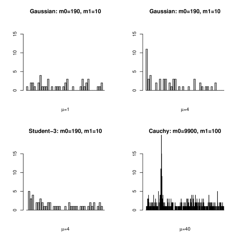
Figure 1: The plots show the counts in the bins of width $1/m$ up to the value of 0.2. The plots on the left show examples without clusters. The counts of null $p$-values in the filter intervals form a Poisson process, whose maxima grow very slowly with $(1-\varepsilon)m$ and are around 4 to 5 in all cases shown. The plots on the right exhibit clear clusters.

2.4 Behavior for long-tailed distributions

In contrast to the Gaussian case, the following results covers a long-tailed distribution and with a filter that is easier to analyze. The “random filter” also uses a regular grid with intervals of length $1/m_{\xi}$. It operates by deleting one randomly chosen $p$-value from each non-empty interval. A random filter deletes less than $m_{\xi}$ $p$-values because of empty intervals. Since the gaps between the ordered uniform $p$-values have a beta$(1,(1-\varepsilon)m)$ distribution, the probability of a gap larger than $2/m_{\xi}$ is equal to $(1-2/m_{\xi})^{(1-\varepsilon)m}\approx\exp(-2(1-\varepsilon)/(1-\xi))$. Gaps of this size imply at least one empty interval.

The result shows that the uniform filtering works as required, but the range of detectability changes. The next result shows that the randomised filtering procedure essentially preserves the true alternatives in the limit as $m\to\infty$. The tight clustering of the $p$-values from the alternatives are responsible for this result.

Theorem 1 (Asymptotic filtering)

We consider the standard Cauchy mixture model,

$$(1-\varepsilon_{m})C(x)+\varepsilon_{m}C(x-\mu_{m})\,,$$

where $\varepsilon_{m}=m^{-\gamma}$ and $\mu_{m}=m^{r}$. If the parameters $(\gamma,r)$ satisfy

$$0<\gamma\text{ and }r>1-\frac{\gamma}{2}\,,$$

it follows that if we use the “random filter” with parameter $\xi$, the expected fraction of the number $\text{FE}_{\xi}$ of falsely deleted alternatives among all true alternatives $\varepsilon_{m}m$ converges to zero, that is,

$$\frac{\mathbb{E}(\text{FE}_{\xi})}{\varepsilon_{m}m}\longrightarrow 0,\quad m\to\infty,$$

Proof 1

The expected value of the false exclusions is

$$\mathbb{E}(\text{FE}_{\xi})=\mathbb{E}\left(\sum_{i:\,H_{i}=1}\textbf{1}\left\{P_{i}\in\mathscr{D}\right\}\right)\,,$$

where 1 denotes an indicator function and $\mathscr{D}$ the random set of deleted $p$-values. With the filter intervals $\left\{I_{j},\;j=1,\ldots,m_{\xi}\right\}$ on $[0,1]$ and their mid-points $c_{j}$, we obtain

$$\mathbb{E}(\text{FE}_{\xi}) =\sum_{i:\,H_{i}=1}\sum_{j=1}^{m_{\xi}}\mathbb{P}\left(P_{i}\in(\mathscr{D}\cap I_{j})\right)=\varepsilon_{m}m\sum_{j=1}^{m_{\xi}}\frac{\varepsilon_{m}f_{P}(c_{j})}{(1-\varepsilon_{m})+\varepsilon_{m}f_{P}(c_{j})}+O(1/m)$$

$$=\varepsilon_{m}mm_{\xi}\int_{0}^{1}\frac{\varepsilon_{m}f_{P}(t)}{(1-\varepsilon_{m})+\varepsilon_{m}f_{P}(t)}\,\text{d}t+O(1/m)=\varepsilon_{m}\varepsilon_{m}mm_{\xi}\int_{0}^{1}\frac{1}{(1-\varepsilon_{m})\frac{1}{f_{P}(t)}+\varepsilon_{m}}\,\text{d}t.$$

Since the function $1/f_{P}$ is bounded on $[0,1]$ and has a single peak at

$$\frac{1}{\pi}\left(\arctan\left(-\sqrt{1+\frac{\mu^{2}}{4}}-\frac{\mu}{2}\right)\right)+1\geq\frac{1}{2}\,,$$

we have the integral over $[0,1]$ upper bounded by twice the integral over the right half. Thus,

$$\mathbb{E}(\text{FE}_{\xi}) \leq 2\varepsilon_{m}m_{\xi}\varepsilon_{m}m\int_{\frac{1}{2}}^{1}\frac{1}{(1-\varepsilon_{m})\frac{1+\left(\tan(\pi/2-\pi t)-\mu\right)^{2}}{1+\tan^{2}(\pi/2-\pi t)}+\varepsilon_{m}}\,\text{d}t$$

$$=\frac{2\varepsilon_{m}^{2}m_{\xi}m}{\pi}\int_{0}^{\frac{\pi}{2}}\frac{1}{(1-\varepsilon_{m})\frac{1+\left(\tan x+\mu\right)^{2}}{1+\tan^{2}x}+\varepsilon_{m}}\,\text{d}x$$

$$\leq\frac{2\varepsilon_{m}^{2}m_{\xi}m}{\pi}\int_{0}^{\frac{\pi}{2}}\frac{1}{(1-\varepsilon_{m})(1+\mu^{2})\cos^{2}x+\varepsilon_{m}}\,\text{d}x$$

$$=\frac{2\varepsilon_{m}^{2}m_{\xi}m}{\pi}\int_{0}^{\frac{\pi}{2}}\frac{\sec^{2}x}{(1-\varepsilon_{m})(1+\mu^{2})+\varepsilon_{m}(1+\tan^{2}x)}\,\text{d}x$$

$$=\frac{2\varepsilon_{m}^{2}m_{\xi}m}{\pi}\int_{0}^{\infty}\frac{1}{(1-\varepsilon_{m})(1+\mu^{2})+\varepsilon_{m}+\varepsilon_{m}y^{2}}\,\text{d}y$$

$$=\frac{2\varepsilon_{m}^{2}m_{\xi}m}{\pi}\frac{1}{(1-\varepsilon_{m})(1+\mu^{2})+\varepsilon_{m}}\int_{0}^{\infty}\frac{1}{1+\left(\frac{\sqrt{\varepsilon_{m}}y}{\sqrt{(1-\varepsilon_{m})(1+\mu^{2})+\varepsilon_{m}}}\right)^{2}}\,\text{d}y$$

$$=\varepsilon_{m}^{2}m_{\xi}m\frac{1}{\sqrt{\varepsilon_{m}}\sqrt{(1-\varepsilon_{m})(1+\mu^{2})+\varepsilon_{m}}}\,.$$

Recall that we consider the parametrisation

$$\varepsilon_{m}=m^{-\gamma},\quad\mu_{m}=m^{r}\,.$$

Therefore, the expected proportion satisfies

$$\frac{\mathbb{E}(\text{FE}_{\xi})}{\varepsilon_{m}m}\leq\frac{\sqrt{\varepsilon_{m}}m_{\xi}}{\sqrt{(1-\varepsilon_{m})(1+\mu^{2})+\varepsilon_{m}}}=\frac{1-\xi}{m^{r+\gamma/2-1}(1+o(1))}\longrightarrow 0$$

as $m\to\infty,$ if

$$r>1-\frac{\gamma}{2}.$$

Theorem 2

Consider the Cauchy mixture model for the test statistics with $\varepsilon_{m}=m^{-\gamma}$ for $0.5<\gamma<1$ and $\mu_{m}=m^{r}$. Let $P_{1},\ldots,P_{m}$ be an i.i.d. sample of $p$-values from this model and apply the fixed-length filter deleting $m_{\xi}=\lceil(1-\xi)m\rceil$ of the $p$-values. If

$$r>1-\frac{\gamma}{2}\,,$$

it follows that

$$\frac{\mathbb{E}\,(\text{FE})}{m\varepsilon_{m}}\longrightarrow 0,\quad m\to\infty\,.$$

Proof 2

The sequence of deleted $p$-values, $\left\{P_{j}^{\xi},\;j=1,\ldots,m_{\xi}\right\}$ forms a partition on $(0,1]$, which we denote by

$$I_{j}^{*}=\left(P_{(j-1)}^{\xi},\;P_{(j)}^{\xi}\right],\quad j=1,\ldots,m_{\xi}+1,$$

with $P_{(0)}^{\xi}=0$ and $P_{(m_{\xi}+1)}^{\xi}=1$. Let $\left\{c_{j}^{*},\;j=1,\ldots,m_{\xi}+1\right\}$ be the mid-points. It follows that

$$\frac{\mathbb{E}\,\big{|}\mathrm{FE}_{\xi}\big{|}}{\varepsilon_{m}m} =\frac{1}{\varepsilon_{m}m}\mathbb{E}\sum_{i:\,H_{i}=1}\textbf{1}\left\{P_{i}\in\mathscr{D}\right\}$$

$$=\frac{1}{\varepsilon_{m}m}\sum_{i:\,H_{i}=1}\sum_{j=1}^{m_{\xi}+1}\mathbb{P}\left(P_{i}\in(\mathscr{D}\cap I_{j}^{*})\right)$$

$$=\sum_{j=1}^{m_{\xi}+1}\frac{\varepsilon_{m}f_{P}(c^{*}_{j})}{(1-\varepsilon_{m})+\varepsilon_{m}f_{P}(c^{*}_{j})}+O(1/m)$$

$$=(m_{\xi}+1)\int_{0}^{1}\frac{\varepsilon_{m}f_{P}(t)}{(1-\varepsilon_{m})+\varepsilon_{m}f_{P}(t)}\,\text{d}t+O(1/m)$$

$$=\varepsilon_{m}(m_{\xi}+1)\int_{0}^{1}\frac{1}{(1-\varepsilon_{m})\frac{1}{f_{P}(t)}+\varepsilon_{m}}\,\text{d}t$$

$$=\frac{1-\xi}{m^{r+\gamma/2-1}(1+o(1))}\longrightarrow 0,\quad m\longrightarrow\infty,$$

if $r>1-\frac{\gamma}{2}\,,$ which is the same asymptotic boundary as (1).

’

3 A multiple test based on uniform filtering

In this section, we show how to formalize the filter approach to obtain a multiple testing procedure in situations where a unique mode of the alternative $p$-value density exists. Our method uses the remaining $p$-values after filtering to estimate the mode. We then return to the original sequence of $p$-values and determine the rejection region surrounding the mode in such a manner that the estimated false discovery rate is below a chosen value. Fig. 2 shows an example.

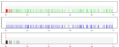
Figure 2: The effect of filtering and the identification of the mode. The plots in the top line show the sample of $p$-values. The red values correspond to the true alternatives. The middle lines show the deleted $p$-values and the bottom line are the remaining ones. The vertical lines indicate the estimated location of the mode.

3.1 Convergence of the filtered mode as $m\to\infty$

Let the unique mode be

$$\vartheta=\underset{t}{\arg\max}\;\tilde{f}_{P}(t)=\underset{t}{\arg\max}\;\left((1-\varepsilon)+\varepsilon f_{P}(t)\right)=\underset{t}{\arg\max}\;f_{P}(t)$$

and let $\{p^{*}_{1},\ldots,p^{*}_{\lfloor\xi m\rfloor}\}$ be the remaining $p$-values after the use of a fixed-length filter.

Assume that the cumulative distribution and the density of the $p$-values under the alternative, namely $F_{P}$ and $f_{P}$, satisfy

1. $F_{P}$ is not concave,

2. $\lim_{t\to 0^{+}}\frac{\text{d}F_{P}(t)}{\text{d}t}=1$,

3. $\lim_{t\to 0^{+}}\frac{\text{d}f_{P}(t)}{\text{d}t}=1$,

4. $f_{P}$ is unimodal,

5. $f_{P}(t)$ is uniformly continuous in $t$.

The filtered $p$-values $\mathscr{F}^{\xi}=\left\{P_{1}^{*},\ldots,P_{\lfloor\xi m\rfloor}^{*}\right\}$ have distribution function $F_{P}^{*}$ and density function $f_{P}^{*}\,.$ We also assume that the density $f_{P}^{*}(t)$ has a unique mode $\vartheta^{\xi}$ defined by

$$f_{P}^{*}(\vartheta^{\xi})=\max_{0\leq t\leq 1}\,f_{P}^{*}(t)\,.$$

With a bandwidth $h$ and the kernel function $K$, the filtered density estimate becomes

$$\hat{f}_{P}^{(\xi,h)}(t)=\frac{1}{h\lfloor\xi m\rfloor}\sum_{j=1}^{\lfloor\xi m\rfloor}K\left(\frac{t-p^{*}_{j}}{h}\right)\,,$$

of which the sample mode will be shown to converge to the true mode.

Definition 1

The random variable $\hat{\vartheta}^{\xi,h}$ such that

$${\hat{f}_{P}}^{(\xi,h)}(\hat{\vartheta}^{\xi,h})=\max_{0\leq t\leq 1}\,{f_{P}}^{(\xi,h)}(t)$$

is called the sample mode.

In kernel density estimation, the bandwidth $h$ balances the bias and the variance of the estimator, which implies that the value of $h$ has to be adapted to the value of $m$. In the following, we consider the situation where $m\to\infty$ with a fixed value of $\xi$ and we assume $h=h(\xi,m)$ satisfies

$$\lim_{\lfloor\xi m\rfloor\to\infty}\,h(\xi,m)=0,\quad\lim_{\lfloor\xi m\rfloor\to\infty}\,\lfloor\xi m\rfloor h^{2}(\xi,m)=\infty.$$ (8)

Theorem 3

Suppose $\hat{\vartheta}^{(\xi,h)}$ is the sample mode and $h=h(\xi,m)$ is a bandwidth satisfying (8). Then $\hat{\vartheta}^{(\xi,h)}\to\vartheta$ in probability.

We use the following propositions to prove the theorem.

Proposition 1 (Unimodal distribution)

For a uniformly continuous and unimodal density on the interval $(0,1)$ with mode $\vartheta$, it follows that, for any $\delta>0$ there exists an $\delta^{\prime}>0$ such that, for $0<t<1,$

$$\left|\vartheta-t\right|\geq\delta\Longrightarrow\left|f(\vartheta)-f(t)\right|\geq\delta^{\prime}\,.$$

Proposition 2

Let $\vartheta^{\xi}$ be the unique mode based on the distribution of the filtered $p$-values $\mathscr{F}^{\xi}$ and $\vartheta$ the mode with respect to the distribution of $p$-values under the alternatives. Then $\vartheta^{\xi}\to\vartheta$ in probability, as $\lfloor\xi m\rfloor\to\infty.$

Proof 3

Proposition 1 is easy to obtain. The proof of Proposition 2 follows from Hoeffding’s inequality applied to

$$\frac{1}{\varepsilon m}\sum_{i:\,H_{i}=1}\textbf{1}\left\{P_{i}\in\mathscr{F}^{\xi}\right\}\,,$$

where $\textbf{1}\left\{P_{i}\in\mathscr{F}^{\xi}\right\}$ are bounded random variables.

The proof of Theorem 3 is as follows.

Proof 4

Consider the density function $f_{P}^{*}(t)$ and the true mode $\vartheta^{\xi}$ based on the distribution of $\mathscr{F}^{\xi}\,.$ Since $\hat{\vartheta}^{(\xi,h)}$ is the sample mode derived from the kernel density estimator after filtration, we prove that

$$\hat{\vartheta}^{(\xi,h)}\to\vartheta^{\xi},\quad\lfloor\xi m\rfloor\to\infty\,.$$

As we assumed that $f_{P}^{*}(t)$ is uniformly continuous and has a unique mode $\vartheta^{\xi}\,,$ it follows that the Proposition 1 holds. Therefore, it is enough to prove the convergence of $f_{P}^{*}(\hat{\vartheta}^{(\xi,h)})$ in probability, that is,

$$f_{P}^{*}(\hat{\vartheta}^{(\xi,h)})\overset{p}{\longrightarrow}f_{P}^{*}(\vartheta^{\xi}),\quad\lfloor\xi m\rfloor\to\infty\,.$$

In order to derive the convergence of the estimated density function, we investigate the characteristic function of the sample. Let $\left\{\varphi_{j}\right\}_{j=1}^{\infty}$ be the sequence of sample characteristic functions,

$$\varphi_{j}(u)=\mathbb{E}\,e^{iuP_{j}^{*}}=\int_{-\infty}^{\infty}e^{iux}\,\text{d}F_{p,j}(x)\,.$$

Correspondingly, we construct the Fourier transform of the kernel function $K$. Suppose we choose a proper kernel $K(u)$ such that the Fourier transform

$$k(t)=\int_{-\infty}^{\infty}e^{itu}K(u)\,\text{d}u$$

is absolutely integrable. Then we derive the kernel density estimator in the form of the sample characteristic function. It follows that the kernel density estimator can be written as

$${\hat{f}_{P}}^{(\xi,h)}(t) =\frac{1}{h\lfloor\xi m\rfloor}\sum_{j=1}^{\lfloor\xi m\rfloor}K\left(\frac{t-P^{*}_{j}}{h}\right)$$

$$=\frac{1}{h}\int K\left(\frac{t-x}{h}\right)\,\text{d}F_{p,\lfloor\xi m\rfloor}(x)=\frac{1}{h}\int K_{h}\left(t-x\right)\,\text{d}F_{p,s}(x),$$

where $K_{h}(t)=K(t/h)\,.$ Let $\mathscr{F}^{\xi}\circ g$ denote the Fourier transform of a function $g$. The Fourier transform of ${f_{P}}_{(h)}(t)$ is then

$$\mathscr{F}^{\xi}\circ{f_{P}}_{(h)}(t) =\frac{1}{h}\mathscr{F}^{\xi}\circ K_{h}(t)\cdot\mathscr{F}^{\xi}\circ F_{p,s}(t)$$

$$=\frac{1}{h}\int K_{h}(ut)e^{iut}\,\text{d}u\cdot\int e^{iut}\,\text{d}F_{p,s}(u)$$

$$=\frac{1}{h}\int K\left(\frac{ut}{h}\right)e^{iut}\,\text{d}u\cdot\int e^{iut}\,\text{d}F_{p,s}(u)$$

$$=\int K(ut)e^{ihut}\,\text{d}u\cdot\int e^{iut}\,\text{d}F_{p,s}(u)$$

$$=k(ht)\varphi_{s}(t)\,,$$

and it follows that the estimator ${\hat{f}_{P}}^{(\xi,h)}(t)$ can be written as

$${\hat{f}_{P}}^{(\xi,h)}(t)=\mathscr{F}^{\xi}\circ\mathscr{F}^{\xi}\circ{f_{P}}_{(h)}(t) =\frac{1}{2\pi}\int e^{-iut}\mathscr{F}^{\xi}\circ{f_{P}}_{(h)}(u)\,\text{d}u$$ (9)

$$=\frac{1}{2\pi}\int e^{-iut}k(hu)\varphi_{s}(u)\,\text{d}u\,.$$

In order to prove the convergence of ${f_{P}}_{h}(t)\,,$ we consider

$$\left|{\hat{f}_{P}}^{(\xi,h)}(t)-f_{P}^{*}(t)\right|^{2}=\left|{\hat{f}_{P}}^{(\xi,h)}(t)-\mathbb{E}[{\hat{f}_{P}}^{(\xi,h)}(t)]+\mathbb{E}[{\hat{f}_{P}}^{(\xi,h)}(t)]-f_{P}^{*}(t)\right|^{2}\,,$$

and we utilise the fact that the kernel density estimate is asymptotically unbiased such that

$$\sup_{t}\left|\mathbb{E}[{\hat{f}_{P}}^{(\xi,h)}(t)]-f_{P}^{*}(t)\right|\longrightarrow 0,\quad s\to\infty\,,$$

so it is enough to prove

$$\sup_{t}\left|{\hat{f}_{P}}^{(\xi,h)}(t)-\mathbb{E}[{\hat{f}_{P}}^{(\xi,h)}(t)]\right|\longrightarrow 0\,.$$ (10)

Following (9), we have

$$\left|{\hat{f}_{P}}^{(\xi,h)}(t)-\mathbb{E}[{\hat{f}_{P}}^{(\xi,h)}(t)]\right| \leq\frac{1}{2\pi}\int\left|e^{iut}k(hu)(\varphi_{s}(u)-\mathbb{E}[\varphi_{s}(u)])\right|\,\text{d}u$$

$$\leq\frac{1}{2\pi}\int|k(hu)|\left|\varphi_{s}(u)-\mathbb{E}[\varphi_{s}(u)]\right|\,\text{d}u\,.$$

Consider the $L^{2}(\mathscr{P})$ norm of (10), it suffices to prove that

$$\mathbb{E}^{\frac{1}{2}}\left[\sup_{t}\left|{\hat{f}_{P}}^{(\xi,h)}(t)-\mathbb{E}[{\hat{f}_{P}}^{(\xi,h)}(t)]\right|^{2}\right]\longrightarrow 0\,.$$

Notice that

$$\mathbb{E}^{\frac{1}{2}}\left[\sup_{t}\left|{\hat{f}_{P}}^{(\xi,h)}(t)-\mathbb{E}[{\hat{f}_{P}}^{(\xi,h)}(t)]\right|^{2}\right] \leq\mathbb{E}^{\frac{1}{2}}\left[\left|\frac{1}{2\pi}\int|k(hu)|\left|\varphi_{s}(u)-\mathbb{E}[\varphi_{s}(u)]\right|\,\text{d}u\right|^{2}\right]$$

$$\leq\frac{1}{2\pi}\int|k(hu)|\,\mathbb{E}^{\frac{1}{2}}\left[\left|\varphi_{s}(u)-\mathbb{E}[\varphi_{s}(u)]\right|^{2}\right]\,\text{d}u\,,$$

which is a straightforward result from Minkowski’s integral inequality and
$\mathbb{E}^{\frac{1}{2}}\left[\left|\varphi_{s}(u)-\mathbb{E}[\varphi_{s}(u)]\right|^{2}\right]$, which is the square root of the variance of $\varphi_{s}(u)$, is bounded by definition

$$\text{Var}(\varphi_{s}(u))=\text{Var}\left(\frac{1}{s}\sum_{j=1}^{s}e^{iuP_{j}^{*}}\right)\leq\frac{1}{s}\mathbb{E}\left|e^{iuP_{j}^{*}}\right|^{2}\leq\frac{1}{s}\,.$$

Therefore,

$$\mathbb{E}^{\frac{1}{2}}\left[\sup_{t}\left|{\hat{f}_{P}}^{(\xi,h)}(t)-\mathbb{E}[{\hat{f}_{P}}^{(\xi,h)}(t)]\right|^{2}\right]\leq\frac{1}{\sqrt{s}h}\int|k(u)|\,\text{d}u\longrightarrow 0$$

if the bandwidth is chosen to satisfy

$$sh^{2}\to 0\,.$$

Thus, (10) is proved and it follows that

$${f_{P}}_{(s,h)}(t)\overset{p}{\longrightarrow}f_{P}^{*}(t),\quad s\to\infty\,,$$

and equivalently, as $m\to\infty.$ By Lemma 1, we conclude that the estimator of the mode with filtration converges to the theoretical mode $\vartheta^{\xi}$ of the filtered $p$-values, and therefore, converges to the mode $\vartheta$.

Remark 1

In order to target the small $p$-values near 0 the transformation of the $p$-values to $-\log(p)$ is a good idea. The kernel density estimator based on the transformed values is more reliable in practice, particularly when the mode of the alternative $p$-values is near zero, as is the case with Gaussian test statistics.

3.2 Finite-sample control of the false discovery rate (FDR)

To capture the alternative $p$-values, We consider rejection regions equal to $\mathscr{R}({\hat{\vartheta}^{(\xi,h)}},\delta)=[\delta_{l},\,\delta_{u}]$ with $\delta_{l}=\hat{\vartheta}^{(\xi,h)}-\delta$ and $\delta_{u}=\hat{\vartheta}^{(\xi,h)}+\delta$, where the half-length is $\delta>0$. The total number of rejections is

$$R=R({\hat{\vartheta}^{(\xi,h)}},\delta)=\#\{i:\,\hat{\vartheta}^{(\xi,h)}-\delta\leq p_{i}\leq\hat{\vartheta}^{(\xi,h)}+\delta\}\,.$$

The choice of $\delta$ is crucial and will be discussed next.

3.2.1 Inference for FDR and pFDR

The pFDR is investigated in Storey [2002], Storey [2003] and Storey et al. [2004] and considers $p$-values generated by a mixture model

$$P_{i}|H_{i}\sim(1-H_{i})\cdot U+H_{i}\cdot F_{P}\,,$$

where the indicators $H_{i}\sim\mathrm{Bernoulli}(\varepsilon)$ are independent random variables. The pFDR of a multiple test with rejection region $\mathscr{R}$ is defined as the conditional probability

$$\mathrm{pFDR}(\mathscr{R})=\mathbb{P}(H_{i}=0|P_{i}\in\mathscr{R})=\frac{m\,(1-\varepsilon)\delta}{m\,\mathbb{P}(P_{i}\in\mathscr{R})}\,.$$ (11)

Here $\delta$ can be any half-width of the rejection interval. The denominator of (11) can be written as

$$\mathbb{P}(P_{i}\in\mathscr{R})=\mathbb{P}(P_{i}\in\mathscr{R}\,|\,R>0)\mathbb{P}(R>0)\,,$$

where $\mathbb{P}(P_{i}\in\mathscr{R}\,|\,R>0)$ can be estimated using the observed value of $R$, that is,

$$\hat{\mathbb{P}}(P_{i}\in\mathscr{R}\,|\,R>0)=\frac{R\vee 1}{m}\,.$$

The probability $\mathbb{P}(R>0)$ depends on the distribution of the test statistics and the multiple testing procedure. For our rejection region $\mathscr{R}({\hat{\vartheta}^{(\xi,h)},\delta})$ we assume that the $p$-values outside of the rejection region are uniformly distributed. This leads to an estimate of $\mathbb{P}(R>0)=1-\mathbb{P}(R=0)\leq 1-(1-\delta)^{m}$.

The pFDR is thus estimated as

$$\widehat{\text{pFDR}}(\mathscr{R}({\hat{\vartheta}^{(\xi,h)}},\delta))=\frac{(1-\hat{\varepsilon})m\delta}{\{R\vee 1\}(1-(1-\delta)^{m})}\,,$$

and the FDR, without conditioning on $R>0$, is estimated by

$$\widehat{\text{FDR}}(\mathscr{R}(\hat{\vartheta}^{(\xi,h)},\delta))=\frac{(1-\hat{\varepsilon})m\delta}{\{R\vee 1\}}\,.$$ (12)

We next consider the estimate of $\varepsilon$.

1. The simplest idea is to avoid estimating $\varepsilon$ by using $1-\varepsilon\leq 1$ in which case the numerator of (12) is estimated by $m\delta$. Although this estimator

   $$\widehat{\mathrm{FDR}}({\hat{\vartheta}^{(\xi,h)}},\delta)=\frac{m\delta}{\{R({\hat{\vartheta}^{(\xi,h)}},\delta)\vee 1\}}$$

   is widely used, and does provide a bound of the FDR control, we seek to have a more precise and more readily interpretable estimate of $\varepsilon$.

2. Based on our filtering procedure, we can select an optimal filtering parameter $\xi$ and use it as an estimator of $\varepsilon$. Suppose the filtering procedure starts with an initial $\xi_{0}=1/2$, estimates the mode and then keeps decreasing the $\xi$-values until the estimate $\hat{\vartheta}$ stabilizes in the sense that the change in the sample mode is smaller than $C$ when changing the $\xi$-value. The second-to-last value of $\xi$ can be then be taken as $\hat{\varepsilon}$. The estimated FDR is

   $$\widehat{\text{FDR}}(\mathscr{R}({\hat{\vartheta}^{(\xi,h)}},\delta))=\frac{(1-\xi)m\delta}{R(\hat{\vartheta}^{(\xi,h)},\delta)\vee 1}\,.$$

3. Storey [2002] introduced the estimator based on a fixed rejection region pre-specified by a tuning parameter $\lambda\in(0,1)$, which is given by

   $$1-\hat{\varepsilon}=\frac{W(\lambda)}{(1-\lambda)m}\,,$$

   where $W(\lambda)=\#\{p_{i}>\lambda\}$ is the number of accepted nulls with the length of acceptance region $1-\lambda.$ The parameter $\lambda$ is selected by minimising the mean square error of the FDR estimator. This estimator was later discussed in Storey [2003], Storey et al. [2004], Genovese and Wasserman [2004], Benjamini et al. [2006] and other related works. Benjamini used this estimator and replaced $m$ by $\hat{m}_{0}=m(1-\hat{\varepsilon})$ in the denominator of the linear step-up threshold, that is, to reject the nulls for the $p$-values $p_{(i)}\leq i\alpha/\hat{m}_{0}.$ Others used this estimator in the inference and control of FDR.

   There are also the methods given by Benjamini and Hochberg [2000], Meinshausen and Rice [2006], Cai et al. [2007], Jin and Cai [2007] that contribute to the estimation of $\varepsilon$, but the estimators are too complicated or not applicable to our study.

We use the estimator of $\varepsilon$ defined by

$$1-\hat{\varepsilon}=\frac{W_{\hat{\vartheta}^{(\xi,h)}}(\xi)}{(1-\xi)m}\,,$$ (13)

which is analogous to Storey’s method, with $W_{\hat{\vartheta}^{(\xi,h)}}(\xi)=\#\left\{|p_{i}-\hat{\vartheta}^{(\xi,h)}|>\xi/2\right\}$. Note that

$$\mathbb{E}(\hat{\varepsilon})=1-\frac{\mathbb{E}(\sum_{i=1}^{m}\textbf{1}\{|p_{i}-\hat{\vartheta}^{(\xi,h)}|>\xi/2\})}{(1-\xi)m}\leq 1-\frac{\mathbb{E}(\sum_{H_{i}=0}\textbf{1}\{|p_{i}-\hat{\vartheta}^{(\xi,h)}|>\xi/2\})}{(1-\xi)m}\\ =1-\frac{(1-\xi)m_{0}}{(1-\xi)m}=\varepsilon\,.$$

Since the simplest structure we assume is the two-point mixture model, we can expect that the $p$-values outside the estimated region $\mathscr{R}_{\vartheta,\xi}$ are dominated by the true nulls with frequency $(1-\varepsilon)(1-\xi)$. In other words, $W_{\hat{\vartheta}^{(\xi,h)}}(\xi)$ is roughly $(1-\xi)(1-\varepsilon)m,$ since the $p$-values from the nulls are assumed to be uniformly distributed outside the rejection region of which the length $1-\delta$ is replaced by $1-\xi\,.$ Thus, $W_{\hat{\vartheta}^{(\xi,h)}}(\xi)/(1-\xi)$ is analogous to $m-R$, and is therefore utilised to estimate $m-\varepsilon m$.

Remark 2

Although we desire to find an accurate estimate of the fraction of the effects, a lower bound of $\varepsilon$ suffices, and the parameter $\xi$ needs not be an estimator of $\varepsilon$. The estimator (13) is slightly biased, and can be used as a lower bound of $\varepsilon$. In reality it is acceptable to claim that the proportion of true alternatives is no less than the declared frequency $\hat{\varepsilon}$ in expectation.

The final estimator of pFDR is

$$\widehat{\text{pFDR}}(\vartheta,\delta)=\frac{W_{\hat{\vartheta}^{(\xi,h)}}(\xi)\delta}{(1-\xi)\{R\vee 1\}(1-(1-\delta)^{m})}\,,$$ (14)

while the FDR (see 12 and 13) is estimated by

$$\widehat{\text{FDR}}(\vartheta,\delta)=\frac{W_{\hat{\vartheta}^{(\xi,h)}}(\xi)\delta}{(1-\xi)\{R(\vartheta,\delta)\vee 1\}}\,.$$ (15)

Based on these estimators we are able to implement the following data-dependent algorithm to detect and locate the alternatives.

1. Compute the $p$-values $p^{m}=\left\{p_{1},\ldots,p_{m}\right\}$ and order them non-decreasingly, i.e. $p_{(1)}\leq p_{(2)}\leq\cdots\leq p_{(m)}.$

2. Apply the fixed length filter $\mathcal{T}^{\text{fixed}}$ with a parameter $0<\xi<1$ to obtain the filtered sequence $\mathscr{F}^{\xi}$.

3. Estimate the density of $\mathscr{F}^{\xi}$ and the mode $\hat{\vartheta}=\hat{\vartheta}^{(\xi,h)}$.

4. Given $i=1,\ldots,m$ and a significance level $\alpha,\,$ reject $H_{0,(i)}$ if $|p_{(i)}-\hat{\vartheta}|\leq|p_{(\tau)}-\hat{\vartheta}|$, where $\tau=\max\left\{\tau:\widehat{\text{FDR}}(\hat{\vartheta},p_{(\tau)}-\hat{\vartheta})\leq\alpha\right\}.$

The control of FDR is based on the estimator (15). The estimator $\hat{\delta}=p_{(\tau)}-\hat{\vartheta}$ is equal the largest half-width of the rejection region $\mathscr{R}(\hat{\vartheta}^{(\xi,h)},\hat{\delta})$ subject to the control of $\widehat{\mathrm{FDR}}$.

3.2.2 Data-dependent control of FDR for finite sample

The following theorem gives some understanding of the estimator of the FDR.

Theorem 4

Based on the rejection region $\mathscr{R}_{\hat{\vartheta}^{(\xi,h)}}$ and The estimator of FDR given by (12) satisfies

$$\mathbf{E}(\widehat{\text{FDR}}(\vartheta,\delta))\geq\mathrm{FDR}(\vartheta,\delta)$$

for any valid $(\vartheta,\delta)$.

Proof 5

We take the difference

$$\mathbb{E}(\widehat{\text{FDR}}(\vartheta,\delta))-\text{FDR}(\vartheta,\delta)=\mathbb{E}\,\left[\frac{\delta W_{\vartheta}(\xi)/(1-\xi)}{\{R(\vartheta,\delta)\vee 1\}}\right]-\mathbb{E}\,\left[\frac{V(\vartheta,\delta)}{\{R(\vartheta,\delta)\vee 1\}}\right]\\ =\mathbb{E}\,\left[\frac{\delta W_{\vartheta}(\xi)/(1-\xi)-V(\vartheta,\delta)}{\{R(\vartheta,\delta)\vee 1\}}\right]\geq\mathbb{E}\,\left[\frac{\delta W_{\vartheta}(\xi)/(1-\xi)-V(\vartheta,\delta)}{R(\vartheta,\delta)}\textbf{1}\left\{R(\vartheta,\delta)>0\right\}\right].$$

Recalling that

$$R(\vartheta,\delta)=S(\vartheta,\delta)+V(\vartheta,\delta),$$

we condition on $S(\vartheta,\delta)$ and tackle the $V(\vartheta,\delta)$ in both the numerator and the denominator. We obtain that the last equation above equals

$$\mathbb{E}\,\left[\frac{\delta W_{\vartheta}(\xi)/(1-\xi)-V(\vartheta,\delta)}{S(\vartheta,\delta)+V(\vartheta,\delta)}\textbf{1}\left\{R(\vartheta,\delta)>0\right\}\right]$$

$$= \mathbb{E}\,\left[\mathbb{E}\left[\frac{\delta W_{\vartheta}(\xi)/(1-\xi)-V(\vartheta,\delta)}{S(\vartheta,\delta)+V(\vartheta,\delta)}\textbf{1}\left\{R(\vartheta,\delta)>0\right\}\Big{|}S(\vartheta,\delta)\right]\right]$$

$$\geq \mathbb{E}\,\left[\frac{\mathbb{E}\left[\left(\delta W_{\vartheta}(\xi)/(1-\xi)-V(\vartheta,\delta)\right)\textbf{1}\left\{R(\vartheta,\delta)>0\right\}\big{|}S(\vartheta,\delta)\right]}{\mathbb{E}\left[(S(\vartheta,\delta)+V(\vartheta,\delta))\textbf{1}\left\{R(\vartheta,\delta)>0\right\}\big{|}S(\vartheta,\delta)\right]}\right]\,,$$

with the last inequality obtained by Jensen’s inequality on $V(\vartheta,\delta)$,  given the fact that

$$\frac{W-V}{S+V}=\frac{W+S}{V+S}-1$$

is a convex function of $V$ with $W+S>0$. Since

$$\mathbb{E}\left[\delta W_{\vartheta}(\xi)/(1-\xi)-V(\vartheta,\delta)\right]\geq\delta m(1-\varepsilon)(1-\xi)/(1-\xi)-m(1-\varepsilon)\delta=0,$$

we conclude that

$$\mathbb{E}(\widehat{\mathrm{FDR}}(\vartheta,\delta))\geq\mathrm{FDR}(\vartheta,\delta)\,.$$

Similarly, we obtain that

$$\mathbb{E}(\widehat{\mathrm{pFDR}}(\vartheta,\delta))\geq\mathrm{pFDR}(\vartheta,\delta)\,,$$

with our estimator having $1-(1-\delta)^{m}\geq\mathbb{P}(R>0)$ in the denominator of (14).

Following this theorem we can get control of the true FDR by limiting the estimated $\widehat{\text{FDR}}(\hat{\vartheta},\delta)$ below a desired level. Our rejection region $\mathscr{R}(\hat{\vartheta},\delta)$ is nested, and the monotonicity of power is guaranteed.

Proposition 3 (Monotonicity of power)

For fixed center $\hat{\vartheta}\,,$ the decision rule defined by the rejection region $\mathscr{R}(\hat{\vartheta},\delta)$ has monotone power in a sense that

$$\beta_{\hat{(}\vartheta,\delta)}\geq\beta_{\hat{(}\vartheta,\delta{{}^{\prime}})}\quad\text{for any}\quad 0<\delta\leq\delta{{}^{\prime}}\leq 2\hat{\vartheta}\,.$$

Remark 3

Storey [2003] also considered the asymptotic control of the FDR and pFDR with $\varepsilon_{m}=\varepsilon$ fixed. We are not interested in this parametrisation since the number of significant components can be moderately large if it is proportional to $m$.

3.3 Numerical results

With $m=1000$ hypotheses, we applied the proposed filtration algorithm to Cauchy mixtures with $\varepsilon=0.05,0.10,0.15,0.20,0.25,$ and $\mu=6,8,10,12,14,16,18,20$. For each configuration we ran $N=200$ replications and get the sample value of the parameters and the true and false discoveries.

Table 2: Simulation results with shifted Cauchy test statistics. The entries show the average values across 1000 replicas for the case of $\varepsilon=$ 0.15. The empirical FDR is fixed at 0.10. The entry for $\widehat{\mathrm{FDR}}$ is the average for the estimated FDR.

$\varepsilon=0.15$	$\mu=6$	$\mu=8$	$\mu=10$	$\mu=12$	$\mu=14$	$\mu=16$	$\mu=18$	$\mu=20$
$\vartheta$	0.05121	0.03899	0.03142	0.02628	0.02258	0.01979	0.01761	0.01586
$\hat{\vartheta}$	0.05193	0.03935	0.03152	0.02636	0.02264	0.01984	0.01763	0.01587
$\hat{\delta}$	0.01573	0.01521	0.01412	0.0139	0.01317	0.01256	0.01241	0.01288
$\widehat{\mathrm{FDR}}$	0.08577	0.09389	0.08816	0.08660	0.08699	0.08493	0.08364	0.08377
FDR	0.08547	0.09238	0.08920	0.08258	0.08364	0.07820	0.07717	0.07451
$\mathrm{TP}/(\varepsilon m)$	0.4924	0.4967	0.5994	0.7506	0.8175	0.8702	0.9006	0.9219

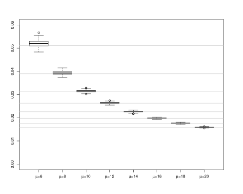
Figure 3: The filtering estimate of the mode of the alternative $p$-values. The estimate is based on the kernel density estimator with the Gaussian kernel and bandwidth tuned to the remaining $p$-values. See also Eq. (6)

The estimates of the alternative mode $\hat{\vartheta}$ are shown in Figure 3. The mode estimates decrease as the shift $\mu$ increases, that is, smaller $p$-values become indicators for true alternatives. A pre-specified level $\alpha=0.1$ is utilised to control the data-dependent estimator $\widehat{\mathrm{FDR}}(\vartheta,\delta)\leq\alpha$ given by (12). We choose the rejection region $\mathscr{R}({\hat{\vartheta},\hat{\delta}})$ with the maximal length $\hat{\delta}$ subject to the control of $\widehat{\mathrm{FDR}}\leq\alpha$. The average FDR is shown in the table by $\widehat{\mathrm{FDR}}$. The true value of FDR computed from the sample is different from the estimator $\widehat{\mathrm{FDR}}(\vartheta,\delta)$, which is influenced by the tuning parameter $\xi$ as we propose in the filtering procedure. With the peak of the $p$-value getting narrow, the rejection region contains more true alternatives.

4 Discussion

4.1 Positive FDR, local FDR and empirical Bayes

In this section we compare our procedures to related ideas and concepts described in Efron et al. [2001], Efron and Tibshirani [2002], Storey [2002], Storey [2003], and Cai and Sun [2017].

pFDR

Storey’s pFDR is also referred to as the posterior FDR, because it applies the Bayes formula to the FDR using the independent Bernoulli model with a common prior probability for $H_{i}=1$. Recall the formula for the pFDR of the rejection region $\mathscr{R}$

$$\mathrm{pFDR}(\mathscr{R})=\mathbb{P}(H_{i}=0|P_{i}\in\mathscr{R})=\frac{(1-\varepsilon)\mathbb{P}(P_{i}\in\mathscr{R}|H_{i}=0)}{(1-\varepsilon)\mathbb{P}(P_{i}\in\mathscr{R}|H_{i}=0)+\varepsilon\mathbb{P}(P_{i}\in\mathscr{R}|H_{i}=1)}\,.$$

This is equivalent to our control of the operating characteristics TPR/FPR, However, Storey and other authors of the related work only discuss the case when $\mathbb{P}(P_{i}\in\mathscr{R}|H_{i}=1)/\mathbb{P}(P_{i}\in\mathscr{R}|H_{i}=0)$ is decreasing, which is the same condition we mentioned for detecting light-tailed alternatives. These papers also limit discussion to the asymptotic cases under the assumption that

$$\sum_{i=1}^{m}(1-H_{i})/m\longrightarrow\pi_{0},\quad m\to\infty,$$

while we consider the asymptotic framework with

$$\sum_{i=1}^{m}(1-H_{i})/m=1-\varepsilon_{m}=1-m^{-\gamma}\longrightarrow 1,\quad m\to\infty.$$

Although the numbers of the true nulls and alternatives both tend to infinity, the ratio will be difficult to detect, which also motivated us to investigate the asymptotically detectable region, that is, detectable clustering in the limit.

Local FDR

The local false discovery rate was originally developed for the $z$-values and uses results from empirical Bayes inference. The $z$-values have densities $f_{0}(z)$ under the nulls and $f_{1}(z)$ under the alternatives with $f_{0}(z)=\varphi(z)=\frac{1}{\sqrt{2\pi}}\mathrm{e}^{-z^{2}/2}$. With the fixed prior probabilities $\pi_{0}$ and $\pi_{1}$, the density of the observed $z$-values is $f(z)=\pi_{0}f_{0}(z)+\pi_{1}f_{1}(z)$. The local Bayes false discovery rate is then defined as

$$\mathrm{Lfdr}(z)=\mathbb{P}(\text{null }|\text{ test statistic }z)=\frac{\pi_{0}f_{0}(z)}{\pi_{0}f_{0}(z)+\pi_{1}f_{1}(z)}\,,$$

where the densities in the numerator and the denominator need to be estimated.

In our work, we consider the distribution of the $p$-values, and we maximise the local ratio TPR(t)/FPR(t) to get the significance center such that a large number of true positives are discovered subject to a small increment of the false positives. We can equivalently define the local FDR for the $p$-values as

$$\mathrm{Lfdr}_{p}(t)=\frac{1-\varepsilon}{1-\varepsilon+\varepsilon\,f_{P}(t)}.$$

Efron’s density estimation makes use of the normal distribution of the $z$-values, whereas we rely on the uniform distribution of the $p$-values from the null hypotheses.

Maximising the local ratio of TPR/FPR is equivalent to minimising the local FDR, taking the Lfdr(t) as a point-wise threshold sequence defined for the $p$-values, and in addition, equivalent to minimising the pFDR as well. We are particularly interested in looking for the most informative region of the $p$-values without a pre-determined rejection rule. Our method is adaptive and data-dependent, and is also interpretable.

4.1.1 Screening for high-throughput data

A filtering method similar to ours appeared in Cai and Sun [2017] for a different purpose. In high-dimensional multiple testing, one of the main issues is to reduce the dimension according to the capacity of the experiments. They discussed a screening approach applied to high-throughput applications, leading to a multi-stage procedure. Their selection rule is defined by the indicator

$$\delta_{i}=\textbf{1}\{\hat{T}(Z_{i})\leq t_{i}\}\,,$$

where $\hat{T}(Z_{i})$ is an estimator of the local FDR and $t_{i}$ is a critical value. The observations with $\delta_{i}=1$ are retained and their paper derives the conditions necessary for a valid screening procedure. They use classic kernel density estimation to estimate the densities and the effectiveness of their estimate Lfdr($z$) depends on the distribution of the test statistics.

4.2 Multi-mode estimation and rejection sets

Consider the mixture model

$$f_{1}(x)=\sum_{j=1}^{k}\pi_{j}f_{0}(x-\mu_{j}),$$

of which the proportions $\pi_{i}$’s and the shifts $\mu_{i}$’s are unknown and not identical. Following the idea of the two-point mixture model, we propose the rejection sets

$$\mathscr{R}=\left\{\bigcup_{i=1}^{k}\mathscr{R}^{(i)}\right\}$$

where $\mathscr{R}^{(i)}=\mathscr{R}_{\vartheta_{i},\delta_{i}}$ is the $i$-th rejection interval.

This problem of detecting clustered alternative components can be converted to a problem of change point detection, as is analysed by Siegmund et al. [2011], Zhang et al. [2010], Cao and Biao Wu [2015] et al.

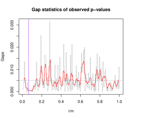
Figure 4: The smoothed gaps of the $p$-values from the Cauchy mixture model.

Instead of detecting the change point in the sequence of $p$-values, we propose an approach to detect the rejection centers based on smoothed gap statistics.

Define a smoothed version of observed $p$-values

$$p_{j}^{\dagger}=\frac{1}{j}\sum_{i=1}^{j}p_{(i)},$$

for $j=1,\ldots,m,$ and let $p_{0}^{\dagger}=p_{(0)}=0.$ For $j=1,\ldots,m$ we define the weighted gap statistic

$$G_{j}^{\dagger} =p_{j}^{\dagger}-p_{j-1}^{\dagger}$$

$$=\frac{(j-1)(p_{(j)}-p_{(j-1)})+(j-2)(p_{(j-1)}-p_{(j-2)})+\cdots+(p_{(2)}-p_{(1)})}{j(j-1)}$$

$$=\frac{(j-1)G_{j-1}+(j-2)G_{j-2}+\cdots+G_{1}}{j(j-1)}\,,$$

which can be re-written as a weighted sum of the original gap statistics $G_{j}=p_{(j)}-p_{(j-1)}$. We give a larger weight to $G_{i}$ as it is closer to $G_{j}^{\dagger},$ which means that the weighted sum of gap statistics capture more precisely the local properties of the $p$-values.

When the observations are i.i.d. from the null distribution, the $p$-values are uniformly distributed, and it follows that $G_{i}=p_{(i)}-p_{(i-1)}\sim\text{Beta}(1,m)$, with expectation $\mathbb{E}(p_{(j)}-p_{(j-1)})=1/(1+m)$. The weighted gaps have a Beta distribution with $\mathbb{E}(G^{\dagger}_{j})=\mathbb{E}(p^{\dagger}_{j}-p^{\dagger}_{j-1})=1/(2+2m)$. Therefore, it is reasonable to compare the weighted gaps to $1/(2+2m)$ and find the region where the cluster of alternative $p$-values occurs, if any.

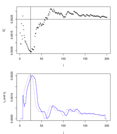
Figure 5: The weighted gaps and the lower and upper local discrepancies

For two-point mixture models, one can intuitively take the $p$-value that minimises the weighted gap, denoted by $\hat{p}_{c}$, to be the center of the cluster from the alternatives. The change point of $G_{j}^{\dagger}$ gives a plausible estimation of the significance center. Formally, define the local discrepancies

$$L_{j}=\left|\frac{1}{k}\sum_{i=j-k}^{j-1}G_{j}^{\dagger}-\frac{1}{2(m+1)}\right|,\quad U_{j}=\left|\frac{1}{k}\sum_{i=j}^{j+k-1}G_{j}^{\dagger}-\frac{1}{2(m+1)}\right|,$$

where $L$ stands for “lower” and $U$ stands for “upper”. We want $L_{j}$ and $U_{j}$ to be sensitive to the change in the distribution of the $p$-value gaps.

Conclusions

The multiple testing literature takes it as a given, that the true alternatives have very small $p$-values. This assumption is wrong in the case of test statistics with long-tailed laws. More general rejection regions can be adaptively selected based on the observed $p$-values. We present such a robust multiple testing procedure and examine its properties. Our approach uses a filter that enlarges the proportion of true alternatives among the filtered $p$-values and then estimates a center for the rejection region by estimating the location of the mode of the filter results. An interval around this center is chosen in order to keep control over the FDR. In some instances, it may be necessary to consider multiple modes in the density of the alternative $p$-values. It would be straightforward to generalize the methods discussed here to this case.

The mode estimator is thus utilised as the mid-point of the central peak of the $p$-values from the alternatives, which in our definition, serves as the significance center of the rejection region $\mathscr{R}.$ Unlike for the Gaussian test procedures, we define the rejection region $\mathscr{R}({\hat{\vartheta},\delta})$ centered at the mode $\hat{\vartheta}$ and of length $\delta$. The center $\hat{\vartheta}$ is estimated by a kernel density estimation applied to the filtered $p$-values, and the length $\delta$ is chosen by data-dependent control of the FDR. We proved that the expected value of the estimator of FDR provides a good upper bound of the true value of the estimated FDR, such that this data-dependent control functions well. In this procedure we do not propose an estimate of $\delta$. An optimal $\hat{\delta}$ is chosen to achieve the maximal power with the estimated $\mathscr{R}({\hat{\vartheta},\hat{\delta}})$ bounded by $\alpha.$

References

- Benjamini and Hochberg [1995] Yoav Benjamini and Yosef Hochberg. Controlling the false discovery rate: a practical and powerful approach to multiple testing. Journal of the Royal Statistical Society: Series B (Statistical Methodology), 57(1):289–300, 1995.
- Benjamini and Hochberg [2000] Yoav Benjamini and Yosef Hochberg. On the adaptive control of the false discovery rate in multiple testing with independent statistics. Journal of Educational and Behavioral Statistics, 25(1):60–83, 2000.
- Benjamini et al. [2006] Yoav Benjamini, Abba M Krieger, and Daniel Yekutieli. Adaptive linear step-up procedures that control the false discovery rate. Biometrika, 93(3):491–507, 2006.
- Cai and Sun [2017] T Tony Cai and Wenguang Sun. Optimal screening and discovery of sparse signals with applications to multistage high-throughput studies. Journal of the Royal Statistical Society: Series B (Statistical Methodology), 79(1):197, 2017.
- Cai et al. [2007] T Tony Cai, Jiashun Jin, and Mark G Low. Estimation and confidence sets for sparse normal mixtures. Annals of Statistics, 35(6):2421–2449, 2007.
- Cao and Biao Wu [2015] Hongyuan Cao and Wei Biao Wu. Changepoint estimation: another look at multiple testing problems. Biometrika, 102(4):974–980, 2015.
- Donoho and Jin [2004] David Donoho and Jiashun Jin. Higher criticism for detecting sparse heterogeneous mixtures. Annals of Statistics, 32(3):962–994, 2004.
- Efron [2004] Bradley Efron. Large-scale simultaneous hypothesis testing: the choice of a null hypothesis. Journal of the American Statistical Association, 99(465):96–104, 2004.
- Efron and Tibshirani [2002] Bradley Efron and Robert Tibshirani. Empirical Bayes methods and false discovery rates for microarrays. Genetic Epidemiology, 23(1):70–86, 2002.
- Efron et al. [2001] Bradley Efron, Robert Tibshirani, John D Storey, and Virginia Tusher. Empirical bayes analysis of a microarray experiment. Journal of the American Statistical Association, 96(456):1151–1160, 2001.
- Fan et al. [2019] Jianqing Fan, Yuan Ke, Qiang Sun, and Wen-Xin Zhou. Farmtest: Factor-adjusted robust multiple testing with approximate false discovery control. Journal of the American Statistical Association, 2019.
- Genovese and Wasserman [2004] Christopher Genovese and Larry Wasserman. A stochastic process approach to false discovery control. Annals of Statistics, 32(3):1035–1061, 2004.
- Ingster [1997] Yuri I. Ingster. Some problems of hypothesis testing leading to infinitely divisible distributions. Mathematical Methods of Statistics, 6:47––69, 1997.
- Jin and Cai [2007] Jiashun Jin and T Tony Cai. Estimating the null and the proportion of nonnull effects in large-scale multiple comparisons. Journal of the American Statistical Association, 102(478):495–506, 2007.
- Meinshausen and Rice [2006] Nicolai Meinshausen and John Rice. Estimating the proportion of false null hypotheses among a large number of independently tested hypotheses. Annals of Statistics, 34(1):373–393, 2006.
- Siegmund et al. [2011] DO Siegmund, NR Zhang, and B Yakir. False discovery rate for scanning statistics. Biometrika, 98(4):979–985, 2011.
- Storey [2002] John D Storey. A direct approach to false discovery rates. Journal of the Royal Statistical Society: Series B (Statistical Methodology), 64(3):479–498, 2002.
- Storey [2003] John D Storey. The positive false discovery rate: a Bayesian interpretation and the -value. Annals of Statistics, 31(6):2013–2035, 2003.
- Storey et al. [2004] John D Storey, Jonathan E Taylor, and David Siegmund. Strong control, conservative point estimation and simultaneous conservative consistency of false discovery rates: a unified approach. Journal of the Royal Statistical Society: Series B (Statistical Methodology), 66(1):187–205, 2004.
- Zhang et al. [2010] Nancy R Zhang, David O Siegmund, Hanlee Ji, and Jun Z Li. Detecting simultaneous changepoints in multiple sequences. Biometrika, 97(3):631–645, 2010.