Isotropy, Clusters, and Classifiers

Abstract

Whether embedding spaces use all their dimensions equally, i.e., whether they are isotropic, has been a recent subject of discussion. Evidence has been accrued both for and against enforcing isotropy in embedding spaces. In the present paper, we stress that isotropy imposes requirements on the embedding space that are not compatible with the presence of clusters—which also negatively impacts linear classification objectives. We demonstrate this fact empirically and use it to shed light on previous results from the literature.

1 Introduction

Recently, there has been much discussion centered around whether vector representations used in NLP do and should use all dimensions equally. This characteristic is known as isotropy: In an isotropic embedding model, every direction is equally probable, ensuring uniform data representation without directional bias. At face value, such a characteristic would appear desirable: Naively, one could argue that an anisotropic embedding space would be overparametrized, since it can afford to use some dimensions inefficiently.

The debate surrounding isotropy was initially sparked by Mu and Viswanath (2018), who highlighted that isotropic static representations fared better on common lexical semantics benchmarks, and Ethayarajh (2019), who stressed that contextual embeddings are anisotropic. Since then, evidence has been accrued both for and against enforcing isotropy on embeddings.

In the present paper, we demonstrate that this conflicting evidence can be accounted for once we consider how isotropy relates to embedding space geometry. Strict isotropy, as assessed by IsoScore (Rudman et al., 2022), requires the absence of clusters, and thereby also conflicts with linear classification objectives. This echoes previous empirical studies connecting isotropy and cluster structures (Ait-Saada and Nadif, 2023, a.o.). In the present paper, we formalize this connection mathematically in Section 2. We then empirically verify our mathematical approach in Section 3, discuss how this relation sheds light on earlier works focusing on anisotropy in Section 4, and conclude with directions for future work in Section 5.

2 Some conflicting optimization objectives

We can show that isotropy—as assessed by IsoScore (Rudman et al., 2022)—impose requirements that conflict with cluster structures—as assessed by silhouette scores (Rousseeuw, 1987)—as well as linear classifier objectives.

Notations.

In what follows, let $\mathcal{D}$ be a multiset of points in a vector space, $\Omega$ a set of labels, and $\ell:\mathcal{D}\to\Omega$ a labeling function that associates a given data-point in $\mathcal{D}$ to the relevant label. For simplicity, let us further assume that $\mathcal{D}$ is PCA-transformed. Let us also define the following constructs for clarity of exposition:

$$\mathcal{D}_{\omega} =\left\{\mathbf{d}~{}:~{}\ell\left(\mathbf{d}\right)=\omega\right\}$$

$$\mathrm{sign}(\omega,\omega^{\prime}) =\begin{cases}-1\qquad\mathrm{if}~{}\omega=\omega^{\prime}\\ +1\hfill\mathrm{otherwise}\end{cases}$$

Simply put, $\mathcal{D}_{\omega}$ is the subset of points in $\mathcal{D}$ with label $\omega$, whereas the $\mathrm{sign}$ function helps delineate terms that need to be maximized (inter-cluster) vs. terms that need to be minimized (intra-cluster).

2.1 Silhouette objective for clustering

We can consider whether the groups as defined by $\ell$ are in fact well delineated by the Euclidean distance, i.e., whether they form natural clusters. This is something that can be assessed through silhouette scores, which involve a separation and a cohesion score for each data-point. The cohesion score consists in computing the average distance between the data-point and other members of its group, whereas separation consists in computing the minimum cohesion score the data-point could have received with any other label than the one it was assigned to. More formally, let:

$$\mathrm{cost}(\mathbf{d},\mathcal{S}) =\frac{1}{|\mathcal{S}|}\sum\limits_{\mathbf{d^{\prime}}\in\mathcal{S}}\sqrt{\sum_{i}\left(\mathbf{d}_{i}-\mathbf{d^{\prime}}_{i}\right)^{2}}$$

then we can define the silhouette for one sample as

$$\mathrm{coh}(\mathbf{d}) =\mathrm{cost}\left(\mathbf{d},\mathcal{D}_{\ell(\mathbf{d})}\setminus\{\mathbf{d}\}\right)$$

$$\mathrm{sep}(\mathbf{d}) =\min\limits_{\omega^{\prime}\in\Omega\setminus\{\ell(\mathbf{d})\}}\mathrm{cost}\left(\mathbf{d},\mathcal{D}_{\omega^{\prime}}\right)$$

$$\mathrm{silhouette}(\mathbf{d}) =\frac{\mathrm{sep}(\mathbf{d})-\mathrm{coh}(\mathbf{d})}{\max\{\mathrm{sep}(\mathbf{d}),\mathrm{coh}(\mathbf{d})\}}$$

Or in other words, the silhouette score is maximized when separation cost ($\mathrm{sep}$) is maximized and cohesion cost ($\mathrm{coh}$) is minimized. Hence, to maximize the silhouette score across the whole dataset $\mathcal{D}$, one needs to (i) maximize all inter-cluster distances, and (ii) minimize all intra-cluster distances.

We can therefore define a maximization objective for the entire set $\mathcal{D}$:

$$\sum\limits_{\mathbf{d}\in\mathcal{D}}\sum\limits_{\mathbf{d^{\prime}}\in\mathcal{D}}\mathrm{sign}(\ell(\mathbf{d}),\ell(\mathbf{d^{\prime}}))\sqrt{\sum_{i}\left(\mathbf{d}_{i}-\mathbf{d^{\prime}}_{i}\right)^{2}}$$

which, due to the monotonicity of the square root in $\mathbb{R}^{+}$, will have the same optimal argument $\mathcal{D}^{\ast}$ as the simpler objective $\mathcal{O}_{\mathrm{S}}$

$$\mathcal{O}_{\mathrm{S}}=\sum\limits_{\mathbf{d}\in\mathcal{D}}\sum\limits_{\mathbf{d^{\prime}}\in\mathcal{D}}\mathrm{sign}(\ell(\mathbf{d}),\ell(\mathbf{d^{\prime}}))\sum_{i}\left(\mathbf{d}_{i}-\mathbf{d^{\prime}}_{i}\right)^{2}$$ (1)

2.2 Incompatibility with IsoScore

How does the objective in (1) conflict with isotropy requirements? Assessments of isotropy such as IsoScore generally rely on the variance vector. As we assume $\mathcal{D}$ to be PCA transformed, the covariance matrix is diagonalized, and we can obtain variance for each individual component through pairwise squared distances (Zhang et al., 2012):

$$\mathbb{V}(\mathcal{D})_{i}=\frac{1}{2|\mathcal{D}|^{2}}\sum\limits_{\mathbf{d}\in\mathcal{D}}\sum\limits_{\mathbf{d^{\prime}}\in\mathcal{D}}\left(\mathbf{d}_{i}-\mathbf{d^{\prime}}_{i}\right)^{2}$$

In IsoScore, this variance vector is then normalized to the length of the $\vec{1}$ vector of all ones, before computing the distance between the two:

$$\sqrt{\sum_{i}\left(\frac{\lVert\vec{1}\rVert_{2}}{\lVert\mathbb{V}(\mathcal{D})\rVert_{2}}\mathbb{V}(\mathcal{D})_{i}-1\right)^{2}}$$

This distance is taken as an indicator of isotropy defect, i.e., isotropic spaces will minimize it.

Given the normalization applied to the variance vector, the defect is computed as the distance between two points on a hyper-sphere. Hence it is conceptually simpler to think of this distance as an angle measurement: Remark that as the cosine between $\mathbb{V}(\mathcal{D})$ and $\vec{1}$ increases, the isotropy defect decreases. In short, to maximize isotropy, we have to maximize the objective $\mathcal{O}_{\mathrm{I}}$

$$\mathcal{O}_{\mathrm{I}} =\cos\left(\vec{1},\mathbb{V}\left(\mathcal{D}\right)\right)$$

$$\propto\sum\limits_{\mathbf{d}\in\mathcal{D}}\sum\limits_{\mathbf{d^{\prime}}\in\mathcal{D}}\sum_{i}\left(\mathbf{d}_{i}-\mathbf{d^{\prime}}_{i}\right)^{2}$$ (2)

This intuitively makes sense: Ignoring vector norms, we have to maximize all distances between every pair of data-points to ensure all dimensions are used equally, i.e., spread data-points out evenly on a hyper-sphere. However, in the general case, it is not possible to maximize both the isotropy objective in (2.2) and the silhouette score objective in (1): Intra-cluster pairwise distances must be minimized for optimal silhouette scores, but must be maximized for optimal isotropy scores. In fact, the two objectives can only be jointly maximized in the degenerate case where no two data-points in $\mathcal{D}$ are assigned the same label.

2.3 Relation to linear classifiers

Informally, latent representations need to form clusters corresponding to the labels in order to optimize a linear classification objective. Consider that in classification problems (i) any data-point $\mathbf{d}$ is to be associated with a particular label $\ell(\mathbf{d})=\omega_{i}$ and dissociated from other labels $\Omega\setminus\{\ell(\mathbf{d})\}$, and (ii) association scores are computed using a dot product between the latent representation to be classified and the output projection matrix, where each column vector $\mathbf{c}^{\omega}$ corresponds to a different class label $\omega$. As such, for any point $\mathbf{d}$ to be associated with its label $\ell(\mathbf{d})$, one has to maximize

In other words, one must either augment the norm of $\mathbf{d}$ or $\mathbf{c}^{\ell(\mathbf{d})}$, or minimize the distance between $\mathbf{d}$ and $\mathbf{c}^{\ell(\mathbf{d})}$. Note however that this does not factor in the other classes $\omega^{\prime}\in\Omega\setminus\{\ell(\mathbf{d})\}$ from which $\mathbf{d}$ should be dissociated, i.e., where we must minimize the above quantity. To account for the other classes, the global objective $\mathcal{O}_{\mathrm{C}}$ to maximize can be defined as

Focusing on the last line, we find that maximizing classification objectives entails minimizing the distance between a latent representation $\mathbf{d}$ and the vector for its label $\mathbf{c}^{\ell(d)}$, and maximizing its distance to all other class vectors.  It is reminiscent of the silhouette score in Equation 1: In particular any optimum for $\mathcal{O}_{\mathrm{C}}$ is an optimum for $\mathcal{O}_{\mathrm{S}}$, since it entails $\mathcal{D}^{\ast}$ such that

$$\forall\mathbf{d},\mathbf{d^{\prime}}\in\mathcal{D}^{\ast}\quad\ell(\mathbf{d})=\ell(\mathbf{d^{\prime}})\iff\mathbf{d}=\mathbf{d^{\prime}}$$

Informally: The cluster associated with a label should collapse to a single point. Therefore the isotropic objective $\mathcal{O}_{\mathrm{I}}$ in Section 2.2 is equally incompatible with the learning objective $\mathcal{O}_{\mathrm{C}}$ of a linear classifier.

In summary,

(i) point clouds cannot both contain well-defined clusters and be isotropic; and (ii) linear classifiers should yield clustered and thereby anisotropic representations.

3 Empirical confirmation

To verify the validity of our demonstrations in Section 2, we can optimize a set of data-points for a classification task using a linear classifier: We should observe an increase in silhouette scores, and a decrease in IsoScore.

3.1 Methodology

We consider four setups: (i) optimizing SBERT sentence embeddings (Reimers and Gurevych, 2019) on the binary polarity dataset of Pang and Lee (2004); (ii) optimizing paired SBERT embeddings on the validation split of SNLI (Bowman et al., 2015); (iii) optimizing word2vec embeddings on POS-tagging multi-label classification using the English CoDWoE dataset (Mickus et al., 2022); and (iv) optimizing word2vec embeddings for WordNet supersenses multi-label classification (Fellbaum, 1998; pre-processed by Tikhonov et al., 2023). For (i) and (ii), we directly optimize the output embeddings of the SBERT model rather than update the parameters of the SBERT model. In all cases, we compute gradients for the entire dataset, and compute silhouette scores with respect to the target labels and IsoScore over 1000 updates. In multi-label cases (iii) and (iv), we consider distinct label vectors as distinct target assignments when computing silhouette scores. Models are trained using the Adam algorithm (Kingma and Ba, 2014); in case (i) and (ii) we optimize cross-entropy, in case (iii) and (iv), binary cross-entropy per label. Remark that setups (ii), (iii) and (iv) subtly depart from the strict requirements laid out in Section 2.

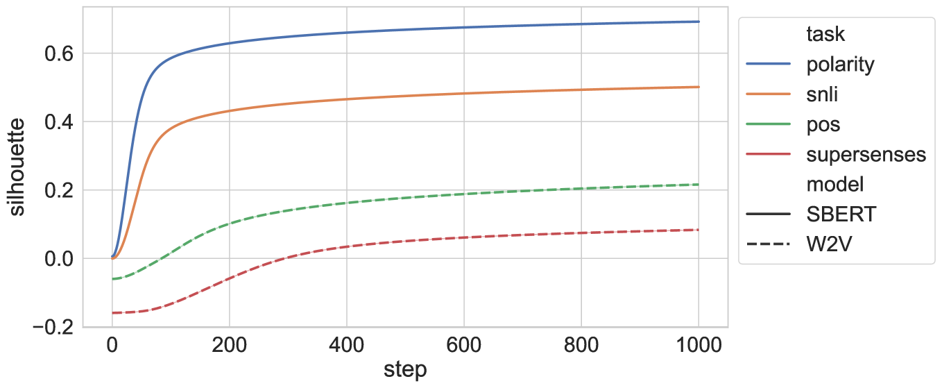
(a) Silhouette across training

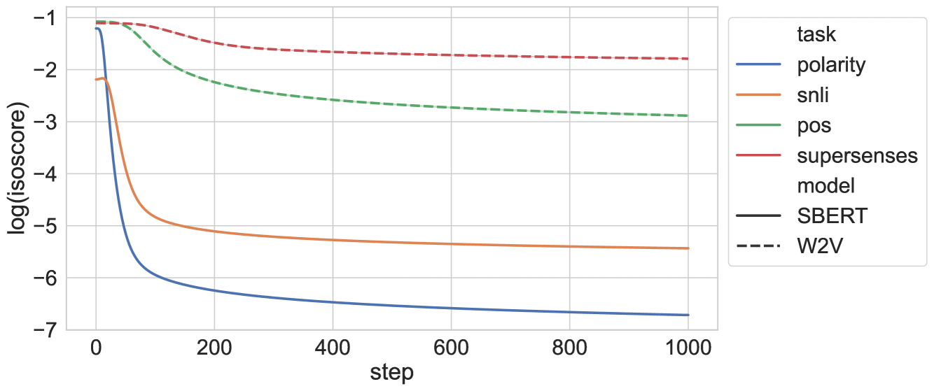
(b) Log-normalized IsoScore across training

Figure 1: Evolution of silhouette score and IsoScore across classification optimization (avg. of 5 runs).

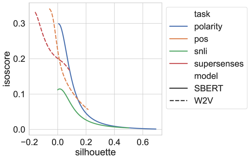
Figure 2: Relationship between silhouette scores and IsoScore (avg. of 5 runs).

3.2 Results

Results of this empirical study are displayed in Figure 1b. Performances with five different random initialization reveal negligible standard deviations (maximum at any step $<0.0054$, on average $<0.0008$). Our demonstration is validated: Across training to optimize classification tasks, the data-points become less isotropic and better clustered. We can also see a monotonically decreasing relationship between IsoScore and silhouette scores, which is better exemplified in Figure 2: We find correlations with Pearson’s $r$ of $-0.808$ for the polarity task, $-0.898$ for SNLI, $-0.947$ for POS-tagging and $-0.978$ for supersense tagging; Spearman’s $\rho$ are always below $-0.998$.

In summary,

we empirically confirm that isotropy requirements conflict with silhouette scores and linear classification objectives.

4 Related works

How does the connection between clusterability and isotropy that we outlined shed light on the growing literature on anisotropy?

While there is currently more evidence in favor of enforcing isotropy in embeddings, the case is not so clear cut that we can discard negative findings, and a vast majority of the positive evidence relies on improper techniques for quantifying isotropy (Rudman et al., 2022). Ethayarajh (2019) stressed that contextual embeddings are effective yet anisotropic. Ding et al. (2022) provides experiments that advise against using isotropy calibration on transformers to enhance performance in specific tasks. Rudman and Eickhoff (2023) finds that anisotropy regularization in fine-tuning appears to be beneficial on a large array of tasks. Lastly, Rajaee and Pilehvar (2021a) find that the contrasts encoded in dominant dimensions can, at times, capture linguistic knowledge.

On the other hand, the original study of Mu and Viswanath (2018) found that enforcing isotropy on static embeddings improved performances on semantic similarity, both at the word and sentence level, as well as word analogy. Subsequently, a large section of the literature has focused on this handful of tasks (e.g., Liang et al., 2021; Timkey and van Schijndel, 2021). Isotropy was also found to be helpful beyond these similarity tasks: Haemmerl et al. (2023) report that isotropic spaces perform much better on cross-lingual tasks, and Jung et al. (2023) stress its benefits for dense retrieval.

These are all applications that require graded ranking judgments, and therefore are generally hindered by the presence of clusters—such clusters would for instance introduce large discontinuities in cosine similarity scores. To take Haemmerl et al. (2023) as an example, note that language-specific clusters are antithetical to the success of cross-lingual transfer applications. It stands to reason that isotropy can be found beneficial in such cases, although the exact experimental setup will necessarily dictate whether it is boon or bane: For instance Rajaee and Pilehvar (2021b) tested fine-tuning LLMs as Siamese networks to optimize performance on sentence-level similarity, and found enforcing isotropy to hurt performances—here, we can conjecture that learning to assign inputs to specific clusters is a viable solution in their case.

The literature has previously addressed the topic of isotropy and clustering. Rajaee and Pilehvar (2021a) advocated for enhancing the isotropy on a cluster-level rather than on a global-level. Cai et al. (2021) confirmed the presence of clusters in the embedding space with local isotropy properties. Ait-Saada and Nadif (2023) investigated the correlation between isotropy and clustering tasks and found that fostering high anisotropy yields high-quality clustering representations. The study presented here provides a mathematical explanation for these empirical findings.

5 Conclusion

We argued that isotropy and cluster structures are antithetical (Section 2), verified that this argument holds on real data (Section 3), and used it to shed light on earlier results (Section 4). This result however opens novel and interesting directions of research: If anisotropic spaces implicitly entail cluster structures, then what is the structure we observe in our modern, highly anisotropic large language models? Prior results suggest that this structure is in part linguistic in nature (Rajaee and Pilehvar, 2021a), but further confirmation is required.

Another topic we intend to pursue in future work concerns the relation between non-classification tasks and isotropy: Isotropy constraints have been found to be useful in problems that are not well modeled by linear classification, e.g. word analogy or sentence similarity. Our present work does not yet offer a thorough theoretical explanation why.

Limitations

The present paper leaves a number of important problems open.

• Our claims with respect to classification are limited to linear classifiers. However, most (if not all) modern deep-learning classification approaches rely on non-linear activation functions across multiple layers of computations. The present demonstration has yet to be expanded to account for such more common cases.

• Our argument focuses on the optima of specific objectives, and says nothing of behavior across training. In particular, we focus on parameters that are optimized for a particular task, but NLP practitioners often verify and measure anisotropy in generalization conditions. In fact, enforcing isotropy could be argued to be a reasonable regularization strategy in that it would lead latent representations to not be tied to a specific classification structure.

• The mathematical formalism is not thorough. For the sake of clarity and given page limitations, we do not include a formal demonstration that the linear classification optimum necessarily satisfies the clustering objective. Likewise, we also rely on the reader’s intuition when discussing isotropy in Section 2.2 (rather than properly deriving it from the relation between the chord from $\vec{1}$ to $\mathbb{V}(\mathcal{D})$ and the sine of the angle between $\vec{1}$ and $\mathbb{V}(\mathcal{D})$), and ignore the cosine denominator.

All of the listed limitations make for good questions to be discussed at length in future work.

Appendix A Responsible NLP Research Checklist Compliance

Dataset	N. items	N. params.
Pang and Lee (2004)	10 662	4 094 976
through nltk (Bird and Loper, 2004)
Bowman et al. (2015)	9 842	4 987 395
from nlp.stanford.edu
Mickus et al. (2022)	11 462	4 341 004
from codwoe.atilf.fr
Fellbaum (1998)	2 275	690 326
from github.com/altsoph

Table 1: Dataset vs. number of datapoints (N. items) and corresponding number of trainable parameters (N. params.).

All the datasets and models we used are English and CC-BY or CC-BY-SA, our use is consistent with the intended use of these resources. We trust original creators of these resources that they contain no personally identifying data. Relevant information is available in Table 1; remark we do not split the data as we are interested on optimization behavior.

Training per model requires between 10 minutes and 1 hour on an RTX3080 GPU; much of which is in fact devoted to CPU computations for IsoScore values. Hyperparameters listed correspond to default PyTorch values (Paszke et al., 2019), no hyperparameter search was carried out. IsoScore is computed with the pip package IsoScore (Rudman et al., 2022), silhouette scores with scikit-learn (Pedregosa et al., 2011).

References

- Ait-Saada and Nadif (2023) Mira Ait-Saada and Mohamed Nadif. 2023. Is anisotropy truly harmful? a case study on text clustering. In Proceedings of the 61st Annual Meeting of the Association for Computational Linguistics (Volume 2: Short Papers), pages 1194–1203, Toronto, Canada. Association for Computational Linguistics.
- Bird and Loper (2004) Steven Bird and Edward Loper. 2004. NLTK: The natural language toolkit. In Proceedings of the ACL Interactive Poster and Demonstration Sessions, pages 214–217, Barcelona, Spain. Association for Computational Linguistics.
- Bowman et al. (2015) Samuel R. Bowman, Gabor Angeli, Christopher Potts, and Christopher D. Manning. 2015. A large annotated corpus for learning natural language inference. In Proceedings of the 2015 Conference on Empirical Methods in Natural Language Processing, pages 632–642, Lisbon, Portugal. Association for Computational Linguistics.
- Cai et al. (2021) Xingyu Cai, Jiaji Huang, Yuchen Bian, and Kenneth Church. 2021. Isotropy in the contextual embedding space: Clusters and manifolds. In International Conference on Learning Representations.
- Ding et al. (2022) Yue Ding, Karolis Martinkus, Damian Pascual, Simon Clematide, and Roger Wattenhofer. 2022. On isotropy calibration of transformer models. In Proceedings of the Third Workshop on Insights from Negative Results in NLP, pages 1–9, Dublin, Ireland. Association for Computational Linguistics.
- Ethayarajh (2019) Kawin Ethayarajh. 2019. How contextual are contextualized word representations? Comparing the geometry of BERT, ELMo, and GPT-2 embeddings. In Proceedings of the 2019 Conference on Empirical Methods in Natural Language Processing and the 9th International Joint Conference on Natural Language Processing (EMNLP-IJCNLP), pages 55–65, Hong Kong, China. Association for Computational Linguistics.
- Fellbaum (1998) Christiane Fellbaum. 1998. WordNet: An Electronic Lexical Database. Bradford Books.
- Haemmerl et al. (2023) Katharina Haemmerl, Alina Fastowski, Jindřich Libovický, and Alexander Fraser. 2023. Exploring anisotropy and outliers in multilingual language models for cross-lingual semantic sentence similarity. In Findings of the Association for Computational Linguistics: ACL 2023, pages 7023–7037, Toronto, Canada. Association for Computational Linguistics.
- Jung et al. (2023) Euna Jung, Jungwon Park, Jaekeol Choi, Sungyoon Kim, and Wonjong Rhee. 2023. Isotropic representation can improve dense retrieval. In Advances in Knowledge Discovery and Data Mining, pages 125–137, Cham. Springer Nature Switzerland.
- Kingma and Ba (2014) Diederik P. Kingma and Jimmy Ba. 2014. Adam: A method for stochastic optimization.
- Liang et al. (2021) Yuxin Liang, Rui Cao, Jie Zheng, Jie Ren, and Ling Gao. 2021. Learning to remove: Towards isotropic pre-trained BERT embedding. In Artificial Neural Networks and Machine Learning – ICANN 2021, pages 448–459, Cham. Springer International Publishing.
- Mickus et al. (2022) Timothee Mickus, Kees Van Deemter, Mathieu Constant, and Denis Paperno. 2022. Semeval-2022 task 1: CODWOE – comparing dictionaries and word embeddings. In Proceedings of the 16th International Workshop on Semantic Evaluation (SemEval-2022), pages 1–14, Seattle, United States. Association for Computational Linguistics.
- Mu and Viswanath (2018) Jiaqi Mu and Pramod Viswanath. 2018. All-but-the-top: Simple and effective postprocessing for word representations. In International Conference on Learning Representations.
- Pang and Lee (2004) Bo Pang and Lillian Lee. 2004. A sentimental education: Sentiment analysis using subjectivity summarization based on minimum cuts. In Proceedings of the 42nd Annual Meeting of the Association for Computational Linguistics (ACL-04), pages 271–278, Barcelona, Spain.
- Paszke et al. (2019) Adam Paszke, Sam Gross, Francisco Massa, Adam Lerer, James Bradbury, Gregory Chanan, Trevor Killeen, Zeming Lin, Natalia Gimelshein, Luca Antiga, Alban Desmaison, Andreas Köpf, Edward Yang, Zach DeVito, Martin Raison, Alykhan Tejani, Sasank Chilamkurthy, Benoit Steiner, Lu Fang, Junjie Bai, and Soumith Chintala. 2019. Pytorch: an imperative style, high-performance deep learning library. In Proceedings of the 33rd International Conference on Neural Information Processing Systems, Red Hook, NY, USA. Curran Associates Inc.
- Pedregosa et al. (2011) F. Pedregosa, G. Varoquaux, A. Gramfort, V. Michel, B. Thirion, O. Grisel, M. Blondel, P. Prettenhofer, R. Weiss, V. Dubourg, J. Vanderplas, A. Passos, D. Cournapeau, M. Brucher, M. Perrot, and E. Duchesnay. 2011. Scikit-learn: Machine learning in Python. Journal of Machine Learning Research, 12:2825–2830.
- Rajaee and Pilehvar (2021a) Sara Rajaee and Mohammad Taher Pilehvar. 2021a. A cluster-based approach for improving isotropy in contextual embedding space. In Proceedings of the 59th Annual Meeting of the Association for Computational Linguistics and the 11th International Joint Conference on Natural Language Processing (Volume 2: Short Papers), pages 575–584, Online. Association for Computational Linguistics.
- Rajaee and Pilehvar (2021b) Sara Rajaee and Mohammad Taher Pilehvar. 2021b. How does fine-tuning affect the geometry of embedding space: A case study on isotropy. In Findings of the Association for Computational Linguistics: EMNLP 2021, pages 3042–3049, Punta Cana, Dominican Republic. Association for Computational Linguistics.
- Reimers and Gurevych (2019) Nils Reimers and Iryna Gurevych. 2019. Sentence-BERT: Sentence embeddings using Siamese BERT-networks. In Proceedings of the 2019 Conference on Empirical Methods in Natural Language Processing and the 9th International Joint Conference on Natural Language Processing (EMNLP-IJCNLP), pages 3982–3992, Hong Kong, China. Association for Computational Linguistics.
- Rousseeuw (1987) Peter J. Rousseeuw. 1987. Silhouettes: A graphical aid to the interpretation and validation of cluster analysis. Journal of Computational and Applied Mathematics, 20:53–65.
- Rudman and Eickhoff (2023) William Rudman and Carsten Eickhoff. 2023. Stable anisotropic regularization.
- Rudman et al. (2022) William Rudman, Nate Gillman, Taylor Rayne, and Carsten Eickhoff. 2022. IsoScore: Measuring the uniformity of embedding space utilization. In Findings of the Association for Computational Linguistics: ACL 2022, pages 3325–3339, Dublin, Ireland. Association for Computational Linguistics.
- Tikhonov et al. (2023) Alexey Tikhonov, Lisa Bylinina, and Denis Paperno. 2023. Leverage points in modality shifts: Comparing language-only and multimodal word representations. In Proceedings of the 12th Joint Conference on Lexical and Computational Semantics (*SEM 2023), pages 11–17, Toronto, Canada. Association for Computational Linguistics.
- Timkey and van Schijndel (2021) William Timkey and Marten van Schijndel. 2021. All bark and no bite: Rogue dimensions in transformer language models obscure representational quality. In Proceedings of the 2021 Conference on Empirical Methods in Natural Language Processing, pages 4527–4546, Online and Punta Cana, Dominican Republic. Association for Computational Linguistics.
- Zhang et al. (2012) Yuli Zhang, Huaiyu Wu, and Lei Cheng. 2012. Some new deformation formulas about variance and covariance. In 2012 Proceedings of International Conference on Modelling, Identification and Control, pages 987–992.