Decentralized Bilevel Optimization over Graphs:
Loopless Algorithmic Update and Transient Iteration Complexity

Abstract

Stochastic bilevel optimization (SBO) is becoming increasingly essential in machine learning due to its versatility in handling nested structures. To address large-scale SBO, decentralized approaches have emerged as effective paradigms in which nodes communicate with immediate neighbors without a central server, thereby improving communication efficiency and enhancing algorithmic robustness. However, current decentralized SBO algorithms face challenges, including expensive inner-loop updates and unclear understanding of the influence of network topology, data heterogeneity, and the nested bilevel algorithmic structures. In this paper, we introduce a single-loop decentralized SBO (D-SOBA) algorithm and establish its transient iteration complexity, which, for the first time, clarifies the joint influence of network topology and data heterogeneity on decentralized bilevel algorithms. D-SOBA achieves the state-of-the-art asymptotic rate, asymptotic gradient/Hessian complexity, and transient iteration complexity under more relaxed assumptions compared to existing methods. Numerical experiments validate our theoretical findings.

1 Introduction

Stochastic bilevel optimization, which tackles problems with nested optimization structures, has gained growing interest. This two-level structure provides a flexible and potent framework for addressing a broad range of tasks, ranging from meta-learning and hyperparameter optimization [21, 54, 4] to reinforcement learning [28], adversarial learning [73], continue learning [5], and imitation learning [2]. State-of-the-art performance in these tasks is typically achieved with extremely large training datasets, which necessitates efficient distributed algorithms for stochastic bilevel optimization across multiple computing nodes.

This paper considers $N$ collaborative nodes connected through a given graph topology. Each node $i$ privately owns a upper-level cost function $f_{i}:\mathbb{R}^{d}\times\mathbb{R}^{p}\rightarrow\mathbb{R}$ and a lower-level cost function $g_{i}:\mathbb{R}^{d}\times\mathbb{R}^{p}\rightarrow\mathbb{R}$. The goal of all nodes is to find a solution to the following distributed stochastic bilevel optimization problem:

$$\min_{x\in\mathbb{R}^{d}}\quad \Phi(x):=f(x,y^{\star}(x)):=\frac{1}{N}\sum_{i=1}^{N}f_{i}\left(x,y^{\star}(x)\right)$$ (1a)

$$\mathrm{s.t.}\quad y^{\star}(x):=\operatorname*{arg\,min}_{y\in\mathbb{R}^{p}}\left\{g(x,y):=\frac{1}{N}\sum_{i=1}^{N}g_{i}(x,y)\right\}$$ (1b)

where local cost functions $f_{i}$ and $g_{i}$ are defined as the expectation of the random function $F(x,y;\xi_{i})$ and $G(x,y;\zeta_{i})$:

$$f_{i}(x,y) :=\mathbb{E}_{\xi_{i}\sim{\mathcal{D}}_{f_{i}}}[F(x,y;\xi_{i})]$$ (2a)

$$g_{i}(x,y) :=\mathbb{E}_{\zeta_{i}\sim{\mathcal{D}}_{g_{i}}}[G(x,y;\zeta_{i})]$$ (2b)

The random variables $\xi_{i}$ and $\zeta_{i}$ represent data samples available at node $i$, following local distributions ${\mathcal{D}}_{f_{i}}$ and ${\mathcal{D}}_{g_{i}}$, respectively. Throughout this paper, we assume local data distributions vary across different nodes, which may result in data heterogeneity issues during the training process.

1.1 Decentralized Bilevel Algorithms

Conventional distributed approaches for solving problem (1) typically adopt a centralized paradigm [29, 63, 56]. In these approaches, a central server is employed to synchronize across the entire network, facilitating the evaluation of a globally averaged upper- or lower-level stochastic gradient for updating the model parameters. This global averaging step can be realized through mechanisms such as Parameter Server [53, 33] or Ring-Allreduce [24]. However, these techniques are associated with either substantial bandwidth costs or high latency [65, Table I], which significantly hampers the scalability of centralized bilevel optimization.

Decentralized bilevel optimization is a new paradigm to approach problem (1), wherein each node maintains a local model updated by communicating with its immediate neighbors. Importantly, decentralized bilevel algorithms eliminate the global averaging step. This distinctive feature results in a noteworthy reduction in communication costs compared to centralized bilevel approaches. Beyond the communication efficiency, decentralized bilevel algorithms also exhibit enhanced robustness to node and link failures, persisting in converging to the desired solution as long as the graph remains connected. In contrast, centralized bilevel algorithms inevitably break down when the central server crashes. For these reasons, considerable research efforts, e.g., [11, 40, 62, 12, 38, 19, 47, 72, 22], have been dedicated to developing decentralized bilevel algorithms with theoretical guarantees and empirical effectiveness.

1.2 Limitations in Existing Literature

Despite the progress in decentralized stochastic bilevel optimization, several key limitations remain in existing results.

1) Expensive inner-loop updates. Tackling the nested optimization structure is challenging. To compute the hypergradient $\nabla_{x}f_{i}(x,y^{\star}(x))$, existing algorithms such as [12, 62, 11, 22, 40] rely on inner-loop updates to assess the lower-level solution $y^{\star}(x)$, as well as the Hessian inverse of $g_{i}(x,y)$. However, these inner-loops are computationally expensive and may incur substantial communication costs, significantly impeding the algorithms’ practicality.

2) Inadequate analysis on non-asymptotic stage. Existing results [40, 62] demonstrate that decentralized and centralized bilevel algorithms exhibit the same asymptotic convergence rate after sufficiently many iterates. However, practical scenarios can only allow a limited number of algorithmic iterations due to the constraints of time or resource budgets and, thus, exhibit decentralization-incurred slowdown in convergence, see Fig. 1 for the illustration. Consequently, it is critical to analyze the non-asymptotic stage and discern when and how decentralized bilevel algorithms get slow. However, existing research falls short in clarifying these questions, as they either overlook the influence of network topologies [40, 11, 12] or neglect the impact of data heterogeneity [62, 22].

3) Unknown distinction between decentralized single-level and bilevel algorithms. The core distinction between decentralized single-level and bilevel optimization resides in their nested two-level structure. Accordingly, a central challenge is to elucidate the impact of this nested structure on the convergence performance. While existing literature demonstrates that decentralized single-level and bilevel algorithms share the same asymptotic convergence rate [40, 62, 22], there remains a notable gap in comprehending how the lower-level optimization influences the more pragmatic non-asymptotic stage, and if it presents substantial challenges in this phase.

Table 1: Comparison between different decentralized stochastic bilevel algorithms. Notation $T$ indicates the number of (outer) iterations, $1-\rho\in(0,1]$ measures the connectivity of the underlying graph, $N$ is the number of computing nodes, $G^{2}$ denotes gradient upper bound, and $b^{2}$ denotes the magnitude of gradient dissimilarity. We also list the result of single-level DSGD in the bottom line for reference.

Algorithm	Single loop	Asymptotic rate◇	Asymptotic grad. complexity†	Transient complexity‡	Assumption◁
DSBO[11]	✗	$\frac{1}{\sqrt{T}}$	$\frac{1}{\varepsilon^{3}}$	N. A.	LC $f_{i}$
MA-DSBO[12]	✗	$\frac{1}{\sqrt{T}}$	$\frac{1}{\varepsilon^{2}}\log(\frac{1}{\varepsilon})$	N. A.	LC $f_{i}$
SLAM[40]	✗	$\frac{1}{\sqrt{NT}}$	$\frac{1}{N\varepsilon^{2}}\log(\frac{1}{\varepsilon})$	N. A.	LC $f_{i}$
Gossip DSBO[62]	✗	$\frac{1}{\sqrt{NT}}$	$\frac{1}{N\varepsilon^{2}}\log(\frac{1}{\varepsilon})$	$\frac{N^{3}G^{4}}{(1-\rho)^{4}}^{\triangleright}$	BG $\nabla f_{i}$
MDBO[22, Thm 1]∗	✗	$\frac{1}{(1-\rho)\sqrt{T}}$	$\frac{1}{(1-\rho)^{2}\varepsilon^{2}}\log(\frac{1}{\varepsilon})$	N. A.	BG $\nabla f_{i}$
MDBO[22, Thm 2]∗	✗	$\frac{1}{\sqrt{NT}}$	$\frac{1}{N\varepsilon^{2}}\log(\frac{1}{\varepsilon})$	$\frac{N^{3}}{(1-\rho)^{8}}$	BG $\nabla f_{i},\nabla g_{i}$
purple!15D-SOBA (ours)	✔	$\boldsymbol{\frac{1}{\sqrt{NT}}}$	$\boldsymbol{\frac{1}{N\varepsilon^{2}}}$	$\boldsymbol{\max\left\{\frac{\rho^{4}N^{3}}{(1-\rho)^{2}},\frac{\rho^{4}N^{3}b^{2}}{(1-\rho)^{4}}\right\}}$	BGD $\nabla f_{i},\nabla g_{i}$
Single-level DSGD [14]	✔	${\frac{1}{\sqrt{NT}}}$	${\frac{1}{N\varepsilon^{2}}}$	${\max\left\{\frac{\rho^{4}N^{3}}{(1-\rho)^{2}},\frac{\rho^{4}N^{3}b^{2}}{(1-\rho)^{4}}\right\}}$	BGD $\nabla f_{i}$

• The asymptotic convergence rate when $T\to\infty$ (smaller is better).

• The number of gradient/Hessian evaluations to achieve an $\varepsilon$-stationary solution when $\epsilon\to 0$ (smaller is better).

• The number of transient iterations an algorithm experiences before the asymptotic rate dominates (smaller is better).

• Additional assumptions beyond convexity, smoothness, and stochastic variance. The bounded gradient dissimilarity (BGD) assumption is much weaker than functions’ Lipschitz continuity (LC) and bounded gradients (BG).

• $G$ is the uniform upper bound of gradients (i.e., $\|\nabla f_{i}\|^{2}\leq G^{2}$) assumed in [62]. It typically holds that $b\ll G$ where $b$ gauges the magnitude of the gradient dissimilarity, i.e., $\frac{1}{N}\sum_{i=1}^{N}\|\nabla f_{i}-\nabla f\|^{2}\leq b^{2}$.

• Asymptotic rate and transient complexity are not given in [22]. We derive them in Appendix B.

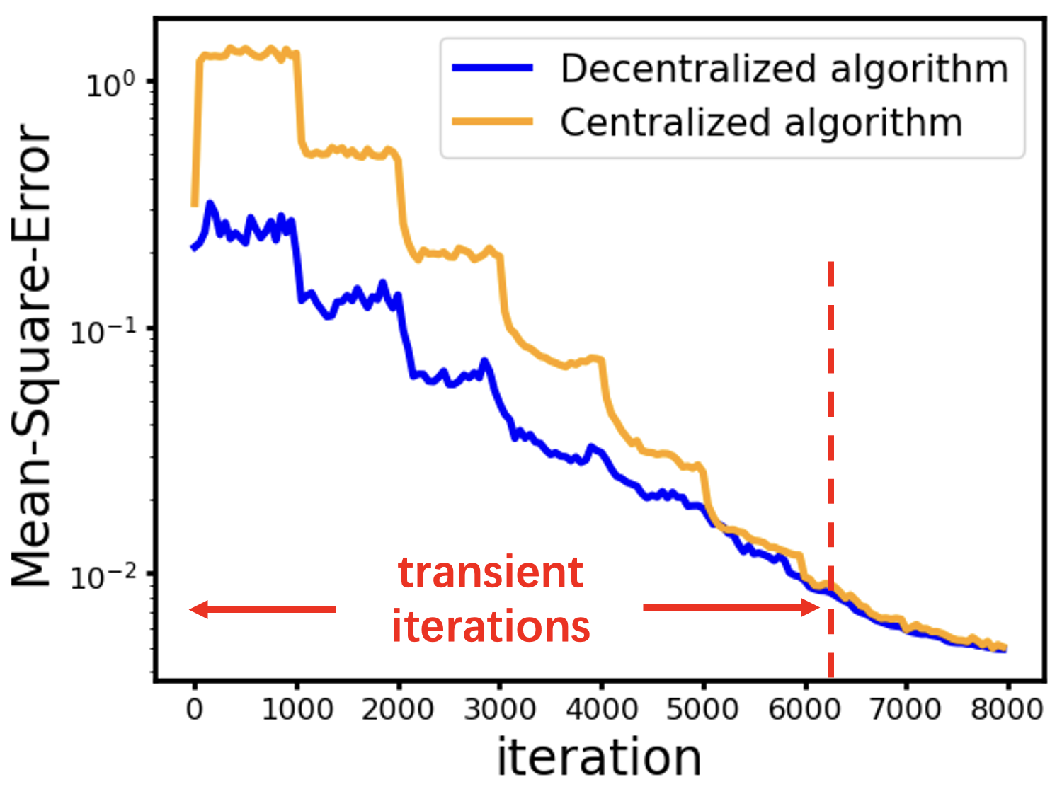
Figure 1: Decentralized algorithm (with stage-wise decaying learning rate) has to experience sufficiently massive transient iterations to achieve the same asymptotic rate as centralized approach.

1.3 Main Results

Transient iteration complexity. While stochastic decentralized bilevel algorithms can asymptotically achieve the same linear speedup rate of $\mathcal{O}(1/\sqrt{NT})$ as their centralized counterparts [40, 62, 22], they require more iterations to reach that stage due to inexact averaging under decentralized communication. Transient iteration complexity refers to the number of iterations a decentralized algorithm has to experience before the asymptotic rate dominates, see Fig. 1 for an illustration. It measures the non-asymptotic stage of decentralized algorithms. A small transient complexity suggests that the decentralized approach can quickly catch up with its centralized counterpart.

Our results. This paper addresses the aforementioned limitations and achieves three main results:

• We propose a single-loop algorithm designed to solve the decentralized stochastic bilevel optimization problem (1), showing the linear-speedup asymptotic convergence ${\mathcal{O}}(1/\sqrt{NT})$ under even more relaxed assumptions than existing methods. Moreover, our algorithm eliminates the need for an inner loop to estimate the lower-level solution $y^{\star}(x)$ or the Hessian inverse of $g_{i}(x,y)$. As a result, we achieve an asymptotic gradient complexity of ${\mathcal{O}}(1/(N\epsilon^{2}))$, surpassing the currently state-of-the-art results by at least a factor of $\log(1/\epsilon)$.

• We provide a thorough non-asymptotic convergence analysis and derive the transient iteration complexity for the proposed algorithm. Our analysis is the first to quantify how network topology and data heterogeneity jointly affect the non-asymptotic convergence stage. It highlights that severe data heterogeneity exacerbates the impact of graph topology, and poorly connected graph topology amplifies the adverse effects of data heterogeneity. Neglecting either one factor would lead to an incomplete non-asymptotic analysis. Furthermore, the transient iteration complexity of our proposed algorithm is smaller, demonstrating faster convergence compared to existing methods.

• We prove that decentralized single-level and bilevel algorithms share the same asymptotic convergence rate as well as the transient iteration complexity. This implies that the nested two-level structure does not pose essential challenges to decentralized bilevel optimization even in the non-asymptotic regime.

All established results in this paper as well as those of existing decentralized stochastic bilevel algorithms are listed in Table 1. Our single-loop algorithm achieves the state-of-the-art asymptotic rate, gradient complexity, and transient iteration complexity under more relaxed assumptions compared to existing methods. Furthermore, our algorithm even achieves the same theoretical convergence properties as single-level DSGD [14].

Orthogonality to variance reduction. In [22, Theorem 3] and [72], the authors employ variance reduction (VR) [49, 31, 15] to enhance decentralized stochastic bilevel algorithms, converging with an asymptotic rate of $\mathcal{O}(T^{-2/3})$ and surpassing all algorithms outlined in Table 1. However, the algorithms in Table 1 are orthogonal to VR, meaning that they can readily incorporate VR to achieve faster convergence. Notably, the utilization of VR is contingent upon more restrictive sample-wise smoothness conditions, e.g., [22, Assumption 7 and 8], we refrain from including [22, Theorem 3] and [72] in Table 1.

1.4 Related Works

Bilevel optimization. Bilevel optimization [6] has extensive applications in operations research, signal processing, and machine learning [57, 71]. A central challenge in bilevel optimization is the estimation of the hypergradient $\nabla\Phi(x)$. To address this, various algorithms have emerged, leveraging approaches such as approximate implicit differentiation [18, 23, 25, 30], iterative differentiation [21, 43, 18, 25, 30], and Neumann series [10, 28]. However, these approaches incur inner-loops to estimate the lower-level solution $y^{\star}(x)$ and the Hessian inverse of $g(x,y)$, resulting in extra computational overhead and worsening the iteration complexity. A recent work [16] develops a novel single-loop framework for stochastic bilevel optimization, in which the Hessian inverse is removed from the algorithmic structure and the lower and upper variables are updated simultaneously. Additionally, various techniques including variance reduction [61, 30, 27] and momentum [9, 13], are employed to attain further enhancements.

Decentralized optimization. Decentralized optimization is useful in situations where the centralized control of all nodes by a single server is either practically infeasible or prohibitively expensive. Early well-known algorithms include decentralized gradient descent [46, 69], diffusion strategies [8], dual averaging [20], EXTRA [51], Exact-Diffusion [70, 34], gradient tracking [60, 17, 45], and decentralized ADMM methods [52, 7]. In the stochastic context, decentralized SGD is established in [35] to achieve the same asymptotic linear speedup as centralized SGD. Since then, many efforts have extended decentralized SGD to directed topologies [3, 44], time-varying topologies [32, 44], and data-heterogeneous scenarios [55, 59, 37, 67, 66, 41]. Lower bounds and optimal complexities are also recently established for stochastic decentralized optimization [42, 68].

Decentralized stochastic bilevel algorithms are studied in [62, 11, 12, 40, 22] with solid theoretical guarantees and strong empirical performance. Nevertheless, these algorithms entail computationally expensive inner-loop updates and often exhibit a limited focus on the non-asymptotic convergence stage in their analyses, as discussed in Sec. 1.2. The comparison between our result and these works is listed in Table 1. Meanwhile, decentralized algorithms [39, 47] are also proposed to solve the personalized bilevel problem:

$$\vspace{-10mm}\min_{x\in\mathbb{R}^{d}} \frac{1}{N}\sum_{i=1}^{N}f_{i}\left(x,y_{i}^{\star}(x)\right),$$ (3)

$$\mathrm{s.t.} y_{i}^{\star}(x):=\operatorname*{arg\,min}_{y\in\mathbb{R}^{p}}g_{i}(x,y),\quad{\forall\,1\leq i\leq N}.\vspace{-5mm}$$

Here, each node has a personalized lower-level cost function, differing from problem (1) where both the upper- and lower-level cost functions are globally averaged.

Concurrent works. Simultaneously and independently, several works [19, 47, 72] have proposed decentralized single-loop bilevel algorithms under various settings. [19] studies the deterministic bilevel optimization problem and establishes an asymptotic rate of $\mathcal{O}(1/\sqrt{T})$, which is worse than our rate ${\mathcal{O}}(T^{-2/3})$ under the same setting, as shown in Theorem 2. Furthermore, it does not clarify the performance under the stochastic settings. Another work [72] employs variance reduction and gradient tracking to address problem (1). While insightful, [72] lacks detailed proofs regarding convergence properties. Reference [47] focuses on the personalized problem (3). In contrast, our algorithm is designed for the more challenging problem (1), which involves handling both the globally averaged upper- and lower-level cost functions. Solving (1) demands substantial efforts to evaluate globally-averaged lower-level gradient in a decentralized manner, a problem not addressed in [72].

2 Preliminaries

Notations. For a second-order differentiable function $f:\mathbb{R}^{d}\times\mathbb{R}^{p}\to\mathbb{R}$, we denote $\nabla_{1}f(x,y)$ and $\nabla_{2}f(x,y)$ as the partial gradients at the $x$’s position and $y$’s position, respectively. Correspondingly, $\nabla_{12}^{2}f(x,y)\in\mathbb{R}^{d\times p}$ and $\nabla_{22}^{2}f(x,y)\in\mathbb{R}^{p\times p}$ represent its partial Jacobian matrix. Differently, we use $\nabla_{x}f(x,y^{\star}(x))$ (resp., $\nabla_{x}^{2}f(x,y^{\star}(x))$) to denote the gradient (resp., Hessian) with respect to $x$ by viewing $y$ as a function of $x$. We let $\|\cdot\|$ denote the $\ell_{2}$ norm of both vectors and matrices, $\|\cdot\|_{F}$ denote the Frobenius norm of a matrix, and $\mathds{1}_{N}\in\mathbb{R}^{N}$ represent the vector with all elements set to $1$. For any local variables $\{x_{i}^{(t)}\}_{i=1}^{n}$, the subscript $i$ (resp, superscript $t$) indicates the index of the node (resp, the iteration) and we write their average $\sum_{i=1}^{N}x_{i}^{(t)}/N$ as $\bar{x}^{(t)}$. We write $a\lesssim b$ if $a\leq Cb$ for a constant $C>0$.

Assumptions. We first list the smoothness condition:

Assumption 1 (Smoothness).

There exist positive constants $L_{\nabla f}$, $L_{\nabla g}$, $L_{\nabla^{2}g}$, $L_{f}$ such that for $1\leq i\leq N$,

1. $\nabla f_{i}$,$\nabla g_{i}$,$\nabla^{2}g_{i}$ are $L_{\nabla f}$, $L_{\nabla g}$, $L_{\nabla^{2}g}$ Lipschitz continuous respectively;

2. $g_{i}(x,\cdot)$ is $\mu_{g}$-strongly convex for any given $x\in\mathbb{R}^{d}$;

3. $\left\|\nabla_{2}f_{i}(x,y^{\star}(x))\right\|\leq L_{f}<\infty$ for all $x\in\mathbb{R}^{d}$ in which $y^{\star}(x)$ is defined in problem (1b).

It is noteworthy that the third condition of Assumption 1 relaxes the restrictive assumptions of Lipschitz continuity of $f$ or, equivalently, the boundedness of $\nabla_{2}f$ used in [22, 40, 13].

Due to the heterogeneity of local data distributions, the local functions $\{(f_{i},g_{i})\}_{i=1}^{N}$ are not identical across different nodes. To tackle this, we assume bounded gradient dissimilarity as follows, which has been widely adopted in prior literature [32, 36].

Assumption 2 (Gradient dissimilarity).

There exists a constant $b\geq 0$ such that for any $(x,y)\in\mathbb{R}^{d}\times\mathbb{R}^{p}$,

$$\dfrac{1}{N}\sum_{i=1}^{N}\left\|\nabla_{1}f_{i}(x,y)-\nabla_{1}f(x,y)\right\|^{2} \leq b^{2},$$ (4a)

$$\dfrac{1}{N}\sum_{i=1}^{N}\left\|\nabla_{2}g_{i}(x,y)-\nabla_{2}g(x,y)\right\|^{2} \leq b^{2},$$ (4b)

$$\dfrac{1}{N}\sum_{i=1}^{N}\left\|\nabla_{22}g_{i}(x,y)-\nabla_{22}g(x,y)\right\|^{2} \leq b^{2}.$$ (4c)

We also make the following standard assumption for stochastic gradients and Hessians.

Assumption 3 (Stochasticity).

There exist constants $\sigma_{f1},\sigma_{g1},\sigma_{g2}\geq 0$ such that for any given $(x,y)\in\mathbb{R}^{d}\times\mathbb{R}^{p}$ and $1\leq i\leq N$,

• the gradient oracles satisfy:

  $$\mathbb{E}_{\xi_{i}\sim{\mathcal{D}}_{f_{i}}}[\nabla_{1}F(x,y;\xi_{i})]=\nabla_{1}f_{i}(x,y),$$

  $$\mathbb{E}_{\zeta_{i}\sim{\mathcal{D}}_{g_{i}}}[\nabla_{2}G(x,y;\zeta_{i})]=\nabla_{2}g_{i}(x,y),$$

  $$\mathbb{E}_{\xi_{i}\sim{\mathcal{D}}_{f_{i}}}\left[\left\|\nabla_{1}F(x,y;\xi_{i})-\nabla_{1}f_{i}(x,y)\right\|^{2}\right]\leq\sigma^{2}_{f1},$$

  $$\mathbb{E}_{\zeta_{i}\sim{\mathcal{D}}_{g_{i}}}\left[\left\|\nabla_{2}G(x,y;\zeta_{i})-\nabla_{2}g_{i}(x,y)\right\|^{2}\right]\leq\sigma^{2}_{g1};$$

• the Jacobian/Hessian oracles satisfy:

  $$\mathbb{E}_{\xi_{i}\sim{\mathcal{D}}_{g_{i}}}\left[\nabla_{12}^{2}G(x,y;\xi_{i})\right]=\nabla_{12}^{2}g_{i}(x,y),$$

  $$\mathbb{E}_{\xi_{i}\sim{\mathcal{D}}_{g_{i}}}\left[\nabla_{22}^{2}G(x,y;\xi_{i})\right]=\nabla_{22}^{2}g_{i}(x,y),$$

  $$\mathbb{E}_{\xi_{i}\sim{\mathcal{D}}_{g_{i}}}\left[\left\|\nabla_{12}^{2}G(x,y;\xi_{i})-\nabla_{12}^{2}g_{i}(x,y)\right\|^{2}\right]\leq\sigma^{2}_{g2},$$

  $$\mathbb{E}_{\xi_{i}\sim{\mathcal{D}}_{g_{i}}}\left[\left\|\nabla_{22}^{2}G(x,y;\xi_{i})-\nabla_{22}^{2}g_{i}(x,y)\right\|^{2}\right]\leq\sigma^{2}_{g2}.$$

This work studies decentralized algorithms over networks of $N$ nodes interconnected by a graph $\mathcal{G}$ with a set of edges $\mathcal{E}$. Node $i$ is connected to node $j$ if $(i,j)\in\mathcal{E}$. To facilitate decentralized communication, we introduce the mixing matrix $W=[w_{i,j}]_{i,j=1}^{N}\in\mathbb{R}^{N\times N}$ in which each weight $w_{i,j}$ scales information flowing from node $j$ to node $i$. Furthermore, we set $w_{i,j}=0$ if $(j,i)\notin\mathcal{E}$. The following standard assumption on the mixing matrix is widely used in [69, 35, 32].

Assumption 4 (Mixing matrix).

The mixing matrix $W$ is doubly stochastic, i.e.,

$$\mathds{1}_{N}^{\top}W=\mathds{1}_{N}^{\top},\quad W\mathds{1}_{N}=\mathds{1}_{N}.$$

Moreover, we assume $\rho:=\left\|W-\mathds{1}_{N}\mathds{1}_{N}^{\top}/N\right\|^{2}\in[0,1)$.

Remark 1 (spectral gap).

In decentralized algorithms, the quantity $1-\rho$ is commonly known as the spectral gap [42, 66] of $W$, which serves as a metric for measuring the connectivity of the network topology. Notably, as $1-\rho\to 1$, it indicates that the topology is well-connected (e.g., for a fully connected graph, the mixing matrix is $W=\mathds{1}_{N}\mathds{1}_{N}^{\top}/N$ with $\rho=0)$. Conversely, as $1-\rho\to 0$, it suggests that the topology is potentially sparse [64, 36].

3 D-SOBA Algorithm

In this section, we present our D-SOBA algorithm for decentralized stochastic bilevel optimization.

Major challenges. The core challenge in stochastic bilevel optimization lies in the estimation of the hypergradient $\nabla\Phi(x)$ (i.e., $\nabla_{x}f(x,y^{\star}(x))$) due to the implicit dependence of $y^{\star}(x)$ on $x$. Under Assumption 1 and the implicit function theory [26], $\nabla\Phi(x)$ is:

$$\nabla\Phi(x)= \ \nabla_{1}f(x,y^{\star}(x))-\Big{(}\nabla^{2}_{12}g(x,y^{\star}(x))\ \cdot$$

$$\left[\nabla^{2}_{22}g(x,y^{\star}(x))\right]^{-1}\cdot\nabla_{2}f(x,y^{\star}(x))\Big{)}$$ (5)

which is computationally expensive due to the need for inverting the partial Hessian. Moreover, the Hessian-inversion

$$\left[\nabla_{22}^{2}g(x,y^{\star}(x))\right]^{-1}=\left[\frac{1}{N}\sum_{i=1}^{N}\nabla_{22}^{2}~{}g_{i}(x,y^{\star}(x))\right]^{-1}$$

cannot be easily accessed through decentralized communication even in the absence of stochastic noise affecting the estimate of $\nabla_{22}^{2}~{}g_{i}(x,y^{\star}(x))$. This challenge can be partially mitigated by incorporating auxiliary inner loops to approximate the lower-level solution $y^{\star}(x)$ and evaluate the Hessian inversion using the Neumann series, as demonstrated in works such as [40, 62, 11, 12]. However, the introduction of these auxiliary inner loops results in sub-optimal convergence, as indicated in Table 1. Additionally, it complicates algorithmic implementation and may impose a substantial burden on communication and computation.

Centralized SOBA. The challenge of Hessian inversion can be effectively addressed by a novel framework known as SOBA. SOBA was initially proposed in [16] as a single-node algorithm. We now extend it to solve the distributed problem (1) in the centralized setup. To begin with, SOBA introduces

$$z^{\star}(x)= \left[\nabla^{2}_{22}g(x,y^{\star}(x))\right]^{-1}\nabla_{2}f(x,y^{\star}(x))$$ (6)

$$= \left[\frac{1}{N}\sum_{i=1}^{N}\nabla_{22}^{2}~{}g_{i}(x,y^{\star}(x))\right]^{-1}\Big{(}\frac{1}{N}\sum_{i=1}^{N}\nabla_{2}f(x,y^{\star}(x))\Big{)}$$

which can be regarded as the solution to minimizing the following distributed optimization problem

$$\!\frac{1}{N}\sum_{i=1}^{N}\left\{\frac{1}{2}z^{\top}\nabla_{22}^{2}g_{i}\left(x,y^{\star}(x)\right)z-z^{\top}\nabla_{2}f_{i}\left(x,y^{\star}(x)\right)\right\}.\!$$ (7)

It is worth noting that while $z^{\star}(x)$ in (6) cannot be written as a finite sum across nodes, problem (7) involves only simple sums. To save computation, we can approximately solve (7) using one-step (stochastic) gradient descent. This, combined with one-step (stochastic) gradient descent to update the upper- and lower-level variables $(x,y)$, forms the centralized single-loop framework for solving problem (1):

$$\mbox{minimize \eqref{eq:upper}:}\quad x^{(t+1)} =x^{(t)}-\frac{\alpha_{t}}{N}\sum_{i=1}^{N}D_{x,i}^{(t)},$$ (8a)

$$\mbox{minimize \eqref{eq:lower}:}\quad y^{(t+1)} =y^{(t)}-\frac{\beta_{t}}{N}\sum_{i=1}^{N}D_{y,i}^{(t)},$$ (8b)

$$\mbox{minimize \eqref{eq:soba}:}\quad z^{(t+1)} =z^{(t)}-\frac{\gamma_{t}}{N}\sum_{i=1}^{N}D_{z,i}^{(t)},$$ (8c)

where $D_{x,i}^{(t)},D_{y,i}^{(t)}$ and $D_{z,i}^{(t)}$ are unbiased estimates of

$$D^{(t)}_{x,i}(x,y,z) =\nabla_{1}f_{i}(x^{(t)},y^{(t)})-\nabla^{2}_{12}~{}g_{i}(x^{(t)},y^{(t)})z^{(t)},$$

$$D^{(t)}_{y,i}(x,y,z) =\nabla_{2}~{}g_{i}(x^{(t)},y^{(t)}),$$

$$D^{(t)}_{y,i}(x,y,z) =\nabla^{2}_{22}~{}g_{i}(x^{(t)},y^{(t)})z^{(t)}-\nabla_{2}f_{i}(x^{(t)},y^{(t)}),$$

respectively, and $\alpha_{t}$, $\beta_{t}$ and $\gamma_{t}$ are learning rates. We denote recursion (8) as centralized SOBA since a central server is required to collect $D_{x,i}^{(t)},D_{y,i}^{(t)}$, and $D_{z,i}^{(t)}$ across the entire network, as well as update variables $x^{(t)},y^{(t)}$ and $z^{(t)}$. It is noteworthy that (8) does not require any inner loop to approximate the lower-level solution $y^{\star}(x)$ or directly evaluate the Hessian inversion of $g(x,y)$.

Decentralized SOBA. Inspired by decentralized gradient descent [46, 8], we extend centralized SOBA (8) to decentralized setup:

$$x_{i}^{(t+1)} =\sum_{j\in{\mathcal{N}}_{i}}w_{ij}\left(x_{j}^{(t)}-\alpha_{t}D_{x,j}^{(t)}\right),$$ (9a)

$$y_{i}^{(t+1)} =\sum_{j\in{\mathcal{N}}_{i}}w_{ij}\left(y_{j}^{(t)}-\beta_{t}D_{y,j}^{(t)}\right),$$ (9b)

$$z_{i}^{(t+1)} =\sum_{j\in{\mathcal{N}}_{i}}w_{ij}\left(z_{j}^{(t)}-\gamma_{t}D_{z,j}^{(t)}\right),$$ (9c)

where $x_{i}^{(t)},y_{i}^{(t)}$ and $z_{i}^{(t)}$ are local variables maintained by each node $i$ at iteration $t$, and $D_{x,i}^{(t)},D_{y,i}^{(t)}$, and $D_{z,i}^{(t)}$ are unbiased estimates of $D_{x,i}^{(t)}(x_{i},y_{i},z_{i}),D_{y,i}^{(t)}(x_{i},y_{i},z_{i})$ and $D_{z,i}^{(t)}(x_{i},y_{i},z_{i})$, respectively. The set $\mathcal{N}_{i}$ includes node $i$ and all its immediate neighbors. We refer to recursion (9) as Decentralized Stochastic One-loop Bilevel Algorithm, or D-SOBA for short. Compared to existing decentralized bilevel algorithms listed in Table 1, D-SOBA eliminates any inner loop that may result in expensive computation, heavy communication, or inferior iteration complexity.

Implementation of D-SOBA is listed in Algorithm 1. For each iteration $t$, we independently sample a minibatch of data $\xi^{(t)}_{i}\sim\mathcal{D}_{f_{i}}$, $\zeta^{(t)}_{i}\sim\mathcal{D}_{g_{i}}$ and computes

$$u_{i,x}^{(t)} :=\nabla_{1}F(x_{i}^{(t)},y_{i}^{(t)};\xi^{(t)}_{i}),$$ (10a)

$$u_{i,y}^{(t)} :=\nabla_{2}F(x_{i}^{(t)},y_{i}^{(t)};\xi^{(t)}_{i}),$$ (10b)

$$v_{i}^{(t)} :=\nabla_{2}G(x_{i}^{(t)},y_{i}^{(t)};\zeta^{(t)}_{i}),$$ (10c)

$$J_{i}^{(t)} :=\nabla^{2}_{12}G(x_{i}^{(t)},y_{i}^{(t)};\zeta^{(t)}_{i}),$$ (10d)

$$H_{i}^{(t)} :=\nabla^{2}_{22}G(x_{i}^{(t)},y_{i}^{(t)};\zeta^{(t)}_{i}).$$ (10e)

These variables are used in Algorithm 1 at each iteration. Furthermore, we impose a moving average on the update of $x_{i}$ in Algorithm 1. As shown in [13], the moving average step enables a more stable and finer-grained direction for estimating hypergradients. We find this strategy plays a crucial role in reducing the order of bias from sample noise in the convergence analysis, as well as relaxing the technical assumptions.

Initialize $x^{(0)}=y^{(0)}=z^{(0)}=h^{(0)}=0$, the values of $\alpha_{t},\beta_{t},\gamma_{t}$ are set properly

for $t=0,1,\cdots,T-1$ do

       for each node $i=1,2,\cdots,N$ in parallel do

             $x_{i}^{(t+1)}:=\sum_{j\in{\mathcal{N}}_{i}}w_{ij}(x_{j}^{(t)}-\alpha_{t}h_{j}^{(t)})$;

            $y_{i}^{(t+1)}:=\sum_{j\in{\mathcal{N}}_{i}}w_{ij}(y_{j}^{(t)}-\beta_{t}v_{j}^{(t)})$;

            $\hat{z}_{i}^{(t+1)}:=z_{i}^{(t)}-\gamma_{t}(H_{i}^{(t)}z_{i}^{(t)}-u_{i,y}^{(t)})$;

            $z_{i}^{(t+1)}:=\sum_{j\in{\mathcal{N}}_{i}}w_{ij}\hat{z}_{j}^{(t+1)}$;

            $\omega_{i}^{(t+1)}:=u_{i,x}^{(t)}-J_{i}^{(t)}z_{i}^{(t)}$;

            $h_{i}^{(t+1)}:=(1-\theta_{t})h_{i}^{(t)}+\theta_{t}\omega_{i}^{(t+1)}$.

      

Algorithm 1 D-SOBA

Other possible algorithmic designs. It is noteworthy that our centralized SOBA (8) serves as a foundation for developing decentralized bilevel algorithms. Rather than relying solely on decentralized gradient descent as in (9), one can leverage techniques such as EXTRA [51], Exact Diffusion [70], gradient tracking [60, 46], and ADMM [52] to develop more advanced decentralized bilevel optimization algorithms. Our theoretical and numerical studies on D-SOBA in this paper serve as the basis for these sophisticated algorithms.

4 Convergence Analysis

We state the convergence guarantees for D-SOBA.

Theorem 1.

Under Assumptions 1, 2, 3, and 4, there exist $c_{1},c_{2},c_{3}>0$ such that if $\alpha_{t}\equiv\Theta(\sqrt{N/T})$, and $\beta_{t}\equiv c_{1}\alpha_{t}$, $\gamma_{t}\equiv c_{2}\alpha_{t}$, $\theta_{t}\equiv c_{3}\alpha_{t}$ for any $0\leq t<T$, then the iterates $\bar{y}^{(t)},\bar{z}^{(t)},\bar{h}^{(t)}$ in D-SOBA satisfy

$$\ \dfrac{1}{T}\sum_{t=0}^{T-1}\mathbb{E}\left[\left\|\bar{y}^{(t)}-\bar{y}^{\star(t)}\right\|^{2}+\left\|\bar{z}^{(t)}-\bar{z}^{\star(t)}\right\|^{2}\right]$$ (11)

$$\lesssim \ \dfrac{1}{T}\sum_{t=0}^{T-1}\mathbb{E}\left[\left\|\bar{h}^{(t)}\right\|^{2}\right]+\dfrac{\alpha}{N}+\dfrac{\rho^{2}\alpha^{2}b^{2}}{(1-\rho)^{2}}+\dfrac{\rho^{2}\alpha^{2}}{(1-\rho)},$$

where $\bar{y}^{\star(t)}$ denotes the minimum of (1b) with respect to $\bar{x}^{(t)}$, and $\bar{z}^{\star(t)}$ denotes the minimum of (7) with respect to $\bar{x}^{(t)},\bar{y}^{\star(t)}$. Furthermore, it also holds that

$$\dfrac{1}{T}\sum_{t=0}^{T-1}\mathbb{E}\left[\left\|\nabla\Phi(\bar{x}^{(t)})\right\|^{2}\right]$$ (12)

$$\lesssim \dfrac{1}{\sqrt{NT}}+\dfrac{\rho^{\frac{2}{3}}}{(1-\rho)^{\frac{1}{3}}T^{\frac{2}{3}}}+\dfrac{\rho^{\frac{2}{3}}b^{\frac{2}{3}}}{(1-\rho)^{\frac{2}{3}}T^{\frac{2}{3}}}+\dfrac{\rho}{(1-\rho)T}+\dfrac{1}{T}.$$

Asymptotic linear speedup. An algorithm is deemed to have reached the linear speedup stage when the term $1/\sqrt{NT}$ dominates the convergence rate [36, 32]. In this regime, algorithms only require $1/(N\varepsilon^{2})$ iterations to achieve an $\varepsilon$-stationary solution, which decreases linearly as the number of computing nodes increases. As demonstrated by (12), D-SOBA attains linear speedup as $T$ becomes sufficiently large. In contrast, algorithms proposed in [11, 12] only achieve a much slower asymptotic rate $1/\sqrt{T}$.

Transient iteration complexity. Transient iteration complexity [48] refers to the number of iterations an algorithm has to experience before reaching its asymptotic linear-speedup stage, that is, iterations $1,\cdots,T$ where $T$ is relatively small so that non-$NT$ terms still dominate the rate. Transient iteration complexity measures the non-asymptotic stage in decentralized stochastic algorithms, see Fig. 1. Many existing works, such as [39, 11, 12], fail to establish the transient iteration complexity as their analysis ignores all non-dominant convergence terms. With fine-grained convergence rate (12), the transient iteration complexity of D-SOBA is:

Corollary 1 (transient iteration complexity).

Under the same assumptions as in Theorem 1, the transient iteration complexity of D-SOBA is (Proof in Appendix A.5)

$$\mathcal{O}\left(\max\left\{\frac{\rho^{4}N^{3}}{(1-\rho)^{2}},\frac{\rho^{4}N^{3}b^{2}}{(1-\rho)^{4}}\right\}\right).$$ (13)

Joint influence of graph and heterogeneity. To our knowledge, Corollary 1 is the first result that quantifies how network topology and data heterogeneity jointly affect the non-asymptotic convergence in decentralized stochastic bilevel optimization. First, expression (13) implies that a sparse topology with $1-\rho\to 0$ can significantly amplify the influence of data heterogeneity $b^{2}$. Second, a large data heterogeneity $b^{2}$ also exacerbates the adverse impact of sparse topologies from ${\mathcal{O}}((1-\rho)^{-2})$ to ${\mathcal{O}}((1-\rho)^{-4})$. Furthermore, expression (13) also implies strategies to improve the transient iteration complexity: developing well-connected graphs with $\rho\to 0$, or developing more effective decentralized algorithms that can remove the influence of $b^{2}$ (e.g., algorithms built upon gradient tracking [1] or Exact-Diffusion [66]). In contrast, existing transient complexities [62, 22] are worse than our established (13), especially when data heterogeneity $b^{2}\to 0$ or $\rho\to 0$, see Table 1 for the detailed comparison.

As effective as single-level DSGD. We find that both the asymptotic rate and transient iteration complexity in D-SOBA are identical to that of single-level decentralized SGD [14]. This implies that the nested lower- and upper-level structure does not pose substantial challenges to decentralized stochastic optimization in terms of both asymptotic rate and transient iteration complexity.

Improved convergence in deterministic scenario. When gradient or Hessian information can be accessed without any noise, i.e., $\sigma_{f1}$, $\sigma_{g1}$, and $\sigma_{g2}$ are all zero, the proposed D-SOBA can attain an enhanced convergence performance. By following the proof argument in Theorem 1, we can readily derive the following result:

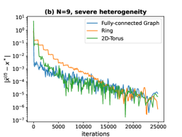
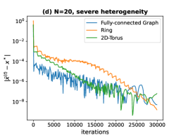
Figure 2: Convergence performance of D-SOBA over various networks under different data heterogeneity.

Corollary 2 (deterministic convergence).

Suppose Assumptions  1, 2, and 4 hold, and variances $\sigma_{f1}=\sigma_{g1}=\sigma_{g2}=0$. D-SOBA achieves (Proof is in Appendix A.5)

$$\dfrac{1}{T}\sum_{t=0}^{T-1}\left\|\nabla\Phi(\bar{x}^{(t)})\right\|^{2}$$ (14)

$$\lesssim \ \dfrac{\rho^{\frac{2}{3}}b^{\frac{2}{3}}}{T^{\frac{2}{3}}(1-\rho)^{\frac{2}{3}}}+\dfrac{\rho^{\frac{2}{3}}}{T^{\frac{2}{3}}(1-\rho)^{\frac{1}{3}}}+\dfrac{\rho}{(1-\rho)T}+\dfrac{1}{T}.$$

Corollary 2 implies that D-SOBA achieves an improved asymptotic rate ${\mathcal{O}}(T^{-2/3})$. In the same deterministic setting, the concurrent single-loop decentralized bilevel algorithm [19] achieves a rate of ${\mathcal{O}}(T^{-1/2}),$ which is inferior to our result. Additionally, it does not clarify the performance under the stochastic settings.

5 Experiments

This section provide experiments to validate our theoretical findings. We first investigate the effects of network topologies and data heterogeneity on D-SOBA with synthetic dataset. Next, we compare D-SOBA with existing decentralized bilevel problems using real-world datasets. Additional details and results can be found in Appendix C.

Synthetic bilevel optimization. We consider problem (1) with the upper- and lower- level loss functions for $1\leq i\leq N$ defined as:

$$f_{i}(x,y) =\mathbb{E}_{\xi_{i},\zeta_{i}}\left[\left(\xi_{i}^{\top}y-\zeta_{i}\right)^{2}\right],$$ (15a)

$$g_{i}(x,y) =\mathbb{E}_{\xi_{i},\zeta_{i}}\left[\left(\xi_{i}^{\top}y-\zeta_{i}\right)^{2}+|x|\|y\|^{2}\right].$$ (15b)

where $y\in\mathbb{R}^{p}$ is the regressed vector and $|x|\geq 0$ is the ridge regularization parameter to be tuned. Each node $i$ observes a sample $(\xi_{i},\zeta_{i})$ in a streaming manner in which $\xi_{i}$ and $\zeta_{i}$ are generated with varying heterogeneity levels (see details in Appendix C.1).

Fig.2 illustrates the performance of our algorithm over three different graphs: the ring graph, the 2D torus graph [64], and the fully-connected graph (i.e., centralized SOBA) with network sizes $N$ of $9$ and $20$. It is observed that for both $N=9$ and $N=20$, the transient stage of D-SOBA over decentralized networks becomes longer as data heterogeneity increases, highlighting the crucial impact of data heterogeneity. Additionally, D-SOBA over the 2D-torus graph exhibits a shorter transient stage than that with the ring graph, indicating that networks with a smaller spectral gap (i.e., worse connectivity) can significantly slow down convergence. Moreover, the transient iterations of both the 2D-torus and ring networks increase as the network size $N$ grows. All these results are consistent with our transient iteration complexity derived in Corollary 1.

Hyperparameter tuning in logistic regression. We consider the hyperparameter tuning problem in logistic regression with the 20 Newsgroup dataset [25]. The problem is formulated as a bilevel stochastic optimization; refer to Appendix C.2 for details on problem formulation and experimental setup.

Fig. 3 compares D-SOBA with MA-DSBO [12] and MDBO [22] over the ring graph under varying data heterogeneity controlled by parameter $h$ (where a large $h$ indicates severe heterogeneity). D-SOBA converges faster and achieves lower upper-level losses and better test accuracy. Moreover, D-SOBA exhibits greater robustness to data heterogeneity, outperforming MA-DSBO and MDBO by significant margins.

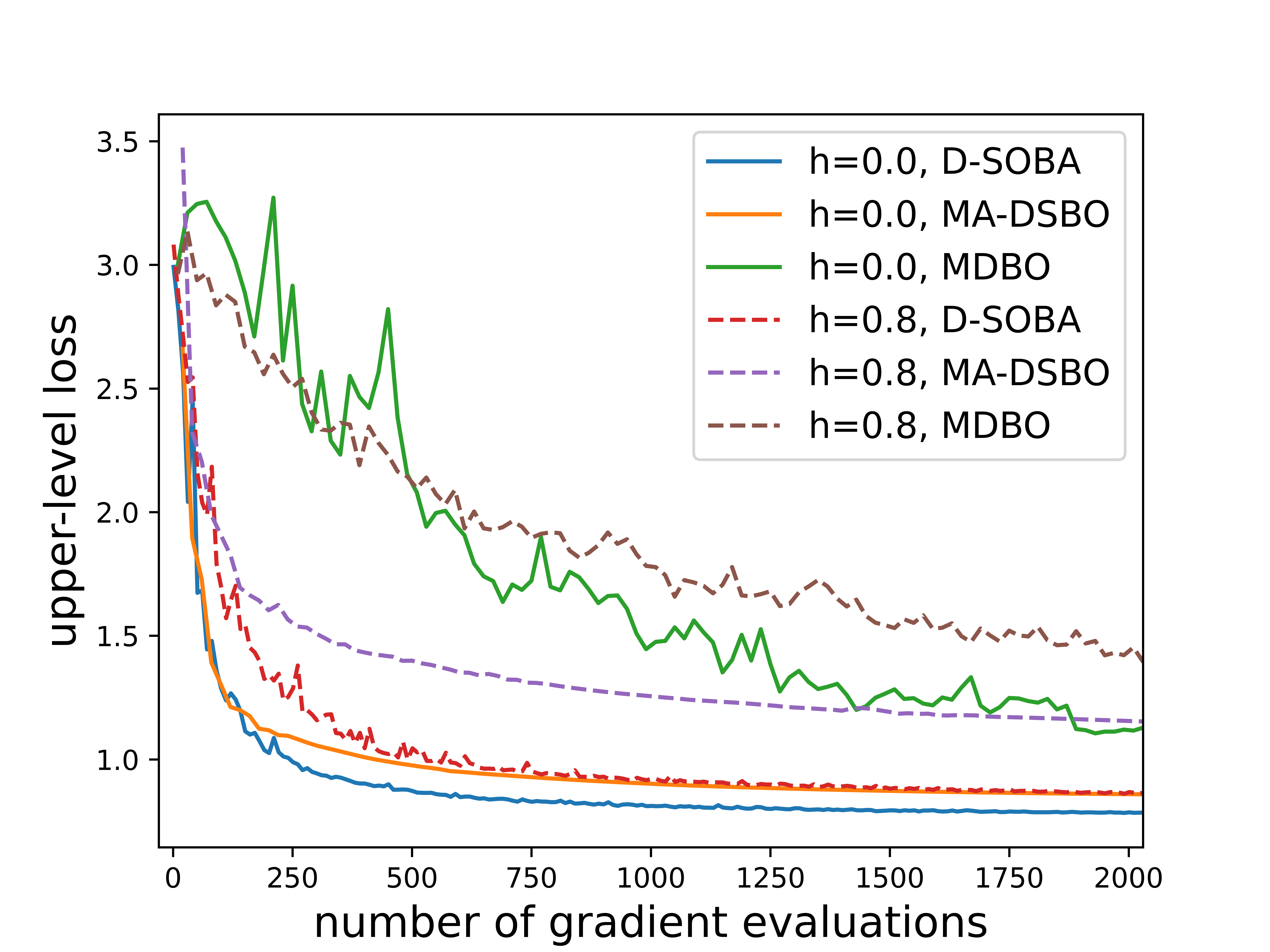
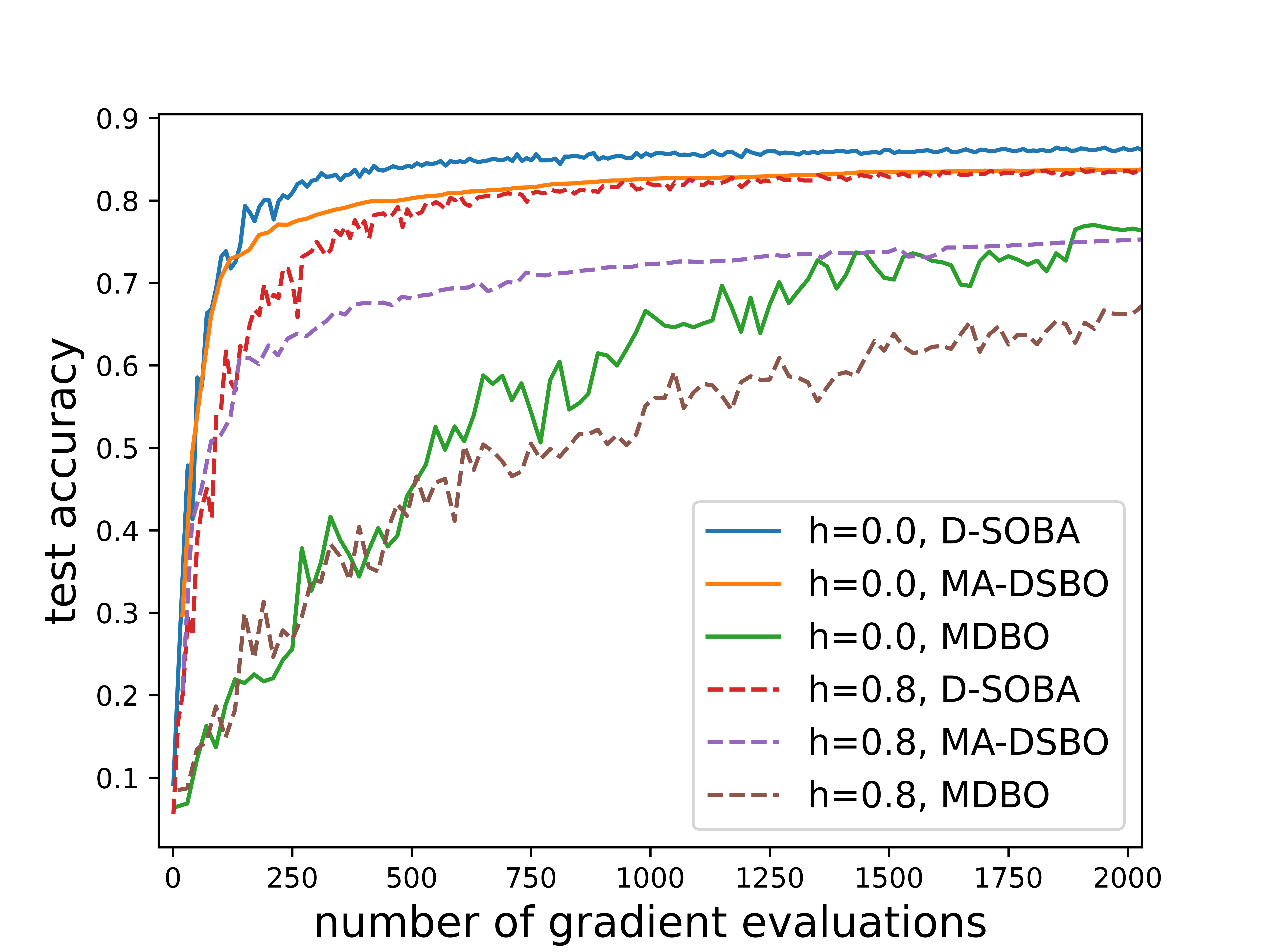
Figure 3: The upper-level loss and test accuracy of D-SOBA, MA-DSBO, and MDBO on logistic regression with the 20 Newsgroup dataset and varying heterogeneity levels.

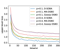
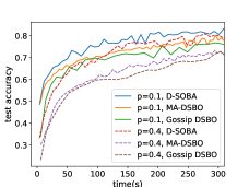
Figure 4: The upper-level loss and test accuracy of D-SOBA, MA-DSBO, and Gossip DSBO on the hyper-cleaning problem with the Fashion MNIST dataset and different corruption rate $p$.

Data hyper-cleaning. We also compare D-SOBA with MA-DSBO [12] and Gossip DSBO [62] on a hyper-cleaning problem with the corrupted Fashion MNIST dataset [58]. Refer to Appendix C.3 for details on problem formulation and experimental setup. Fig. 4 presents the upper-level loss and test accuracy of D-SOBA, MA-DSBO, and Gossip DSBO when the corruption rate $p$ equals 0.1 and 0.4 over an exponential graph [64] with $N=10$ nodes, respectively. We observe that D-SOBA converges faster and achieves higher test accuracy compared to baselines.

More results. More experimental results with varying graph topologies and data heterogeneity are in Appendix C, in which the convergence curves for both the training loss and test accuracy are shown to justify the theoretical findings of this paper.

6 Conclusion and Limitations

This paper introduces D-SOBA, a single-loop decentralized SBO algorithm that achieves state-of-the-art asymptotic convergence rate and gradient/Hessian complexity under more relaxed assumptions compared to existing methods. We also clarify, for the first time, the joint influence of network topology and data heterogeneity on bilevel algorithms through an analysis of transient iteration complexity.

However, D-SOBA relies on the assumption of bounded gradient dissimilarity, which might be violated when local distribution ${\mathcal{D}}_{f_{i}}$ or ${\mathcal{D}}_{g_{i}}$ differs drastically across nodes. As future work, we will explore techniques to mitigate the impact of data heterogeneity, aiming to further enhance the convergence performance of decentralized SBO algorithms.

Appendix A Proof of the Convergence Rate for Algorithm 1.

Here we present the proof of Theorem 1 as well as two corollaries including the transient time and the convergence rate in the deterministic case of Algorithm 1, which provides the theoretical analysis on the convergence of Algorithm 1.

A.1 Notations

At the beginning of the proof, we present some notations which will be used in the proof as follows. Firstly, for $1\leq i\leq N$ and $0\leq t\leq T$, let $y^{(t)}_{i,*}=\mathop{\arg\min}_{y}g(x^{(t)}_{i},y)$ denotes the minimum of (1b) with respect to $x^{(t)}_{i}$, and $z^{(t)}_{i,*}=(\nabla_{22}^{2}g(x^{(t)}_{i},y^{(t)}_{i,*}))^{-1}\nabla_{2}f(x^{(t)}_{i},y^{(t)}_{i,*})$ denotes the minimum of (7) with respect to $x^{(t)}_{i},y^{(t)}_{i,*}$.

Moreover, we introduce $\mathcal{F}^{(t)}=\sigma\left[\bigcup_{\tau=0}^{t}\bigcup_{i=1}^{N}\{x^{(\tau)}_{i},y^{(\tau)}_{i},z^{(\tau)}_{i},h^{(\tau)}_{i}\}\right]$ to denote the $\sigma$-field generated by all items with superscripts in the first $t$ rounds of iterations. From Assumption 3, we have:

$$\mathbb{E}\left[u^{(t)}_{i,x}\middle|\mathcal{F}^{(t)}\right] =\nabla_{1}f_{i}(x^{(t)}_{i},y^{(t)}_{i}),\quad\mathbb{E}\left[\left\|u^{(t)}_{i,x}-\nabla_{1}f_{i}(x^{(t)}_{i},y^{(t)}_{i})\right\|^{2}\middle|\mathcal{F}^{(t)}\right]\leq\sigma_{f1}^{2};$$ (16a)

$$\mathbb{E}\left[u^{(t)}_{i,y}\middle|\mathcal{F}^{(t)}\right] =\nabla_{2}f_{i}(x^{(t)}_{i},y^{(t)}_{i}),\quad\mathbb{E}\left[\left\|u^{(t)}_{i,y}-\nabla_{2}f_{i}(x^{(t)}_{i},y^{(t)}_{i})\right\|^{2}\middle|\mathcal{F}^{(t)}\right]\leq\sigma_{f2}^{2};$$ (16b)

$$\mathbb{E}\left[v^{(t)}_{i}\middle|\mathcal{F}^{(t)}\right] =\nabla_{2}g_{i}(x^{(t)}_{i},y^{(t)}_{i}),\quad\mathbb{E}\left[\left\|v^{(t)}_{i}-\nabla_{2}g_{i}(x^{(t)}_{i},y^{(t)}_{i})\right\|^{2}\middle|\mathcal{F}^{(t)}\right]\leq\sigma_{g1}^{2};$$ (16c)

$$\mathbb{E}\left[J^{(t)}_{i}\middle|\mathcal{F}^{(t)}\right] =\nabla_{12}^{2}g_{i}(x^{(t)}_{i},y^{(t)}_{i}),\quad\mathbb{E}\left[\left\|J^{(t)}_{i}-\nabla_{12}^{2}g_{i}(x^{(t)}_{i},y^{(t)}_{i})\right\|^{2}\middle|\mathcal{F}^{(t)}\right]\leq\sigma_{g2}^{2};$$ (16d)

$$\mathbb{E}\left[H^{(t)}_{i}\middle|\mathcal{F}^{(t)}\right] =\nabla_{22}^{2}g_{i}(x^{(t)}_{i},y^{(t)}_{i}),\quad\mathbb{E}\left[\left\|H^{(t)}_{i}-\nabla_{22}^{2}g_{i}(x^{(t)}_{i},y^{(t)}_{i})\right\|^{2}\middle|\mathcal{F}^{(t)}\right]\leq\sigma_{g2}^{2}.$$ (16e)

Remark. From the definition of $\mathcal{F}^{(t)}$, we know that $h^{(t+1)}_{i}$ and $x^{(t+1)}_{i}$ ($1\leq i\leq N$) are both $\mathcal{F}^{(t)}$-measurable. Then from the update of $x^{(t+1)}_{i}$ in Algorithm 1, we know that $x^{(t+1)}_{i}$ is actually $\mathcal{F}^{(t)}$-measurable.

Then we present the matrix form of iterators on different clients as follows:

$$\mathbf{x}^{(t)} =\left(x^{(t)}_{1},x^{(t)}_{2},\cdots,x^{(t)}_{N}\right)^{\top}_{N\times{d}},\quad\mathbf{\bar{x}}^{(t)}=\left(\bar{x}^{(t)},\bar{x}^{(t)},\cdots,\bar{x}^{(t)}\right)^{\top}_{N\times{d}},$$

$$\mathbf{y}^{(t)} =\left(y^{(t)}_{1},y^{(t)}_{2},\cdots,y^{(t)}_{N}\right)^{\top}_{N\times{p}},\quad\mathbf{\bar{y}}^{(t)}=\left(\bar{y}^{(t)},\bar{y}^{(t)},\cdots,\bar{y}^{(t)}\right)^{\top}_{N\times{p}},$$

$$\mathbf{z}^{(t)} =\left(z^{(t)}_{1},z^{(t)}_{2},\cdots,z^{(t)}_{N}\right)^{\top}_{N\times{d}},\quad\mathbf{\bar{z}}^{(t)}=\left(\bar{z}^{(t)},\bar{z}^{(t)},\cdots,\bar{z}^{(t)}\right)^{\top}_{N\times{d}},$$

$$\mathbf{h}^{(t)} =\left(h^{(t)}_{1}h^{(t)}_{2},\cdots,h^{(t)}_{N}\right)^{\top}_{N\times{d}},$$

$$\mathbb{E}\left[\mathbf{\omega}^{(t)}\middle|\mathcal{F}^{(t-1)}\right] =\left(\mathbb{E}\left[{\omega}_{t,1}\middle|\mathcal{F}^{(t-1)}\right],\mathbb{E}\left[{\omega}_{t,2}\middle|\mathcal{F}^{(t-1)}\right],\cdots,\mathbb{E}\left[{\omega}_{t,N}\middle|\mathcal{F}^{(t-1)}\right]\right)^{\top}_{N\times{p}},$$

$$\overline{\mathbb{E}\left[\mathbf{\omega}^{(t)}\middle|\mathcal{F}^{(t-1)}\right]} =\left(\mathbb{E}\left[\bar{\omega}^{(t)}\middle|\mathcal{F}^{(t-1)}\right],\mathbb{E}\left[\bar{\omega}^{(t)}\middle|\mathcal{F}^{(t-1)}\right],\cdots,\mathbb{E}\left[\bar{\omega}^{(t)}\middle|\mathcal{F}^{(t-1)}\right]\right)^{\top}_{N\times{p}},$$

$$\mathbf{v}^{(t+1)} =\left(v^{(t+1)}_{1},v^{(t+1)}_{2},\cdots,v^{(t+1)}_{N}\right)^{\top}_{N\times{p}},$$

$$\mathbf{p}^{(t+1)} =\left(p^{(t+1)}_{1},p^{(t+1)}_{2},\cdots,p^{(t+1)}_{N}\right)^{\top}_{N\times{p}},$$

$$\nabla_{22}\mathbf{g}^{(t+1)}\times\mathbf{z}^{(t)} =\left(\nabla_{22}g_{1}(x_{1}^{(t)},y_{1}^{(t)})z_{1}^{(t)},\nabla_{22}g_{2}(x_{2}^{(t)},y_{2}^{(t)})z_{2}^{(t)},\cdots,\nabla_{22}g_{N}(x_{N}^{(t)},y_{N}^{(t)})z_{N}^{(t)}\right)^{\top}_{N\times{p}},$$

$$\nabla_{2}\mathbf{f}^{(t+1)} =\left(\nabla_{2}f_{1}(x_{1}^{(t)},y_{1}^{(t)}),\nabla_{2}f_{2}(x_{2}^{(t)},y_{2}^{(t)}),\cdots,\nabla_{2}f_{N}(x_{N}^{(t)},y_{N}^{(t)})\right)^{\top}_{N\times{p}}.$$

$$\nabla_{2}\mathbf{g}^{(t+1)} =\left(\nabla_{2}g_{1}(x_{1}^{(t)},y_{1}^{(t)}),\nabla_{2}g_{2}(x_{2}^{(t)},y_{2}^{(t)}),\cdots,\nabla_{2}g_{N}(x_{N}^{(t)},y_{N}^{(t)})\right)^{\top}_{N\times{p}}.$$

Denote $\Delta_{t}^{2}$ as the consensus error of the $t$-th round of iteration, i.e.,

$$\Delta_{t}^{2}=\left\|\mathbf{x}^{(t)}-\bar{\mathbf{x}}^{(t)}\right\|_{F}^{2}+\left\|\mathbf{y}^{(t)}-\bar{\mathbf{y}}^{(t)}\right\|_{F}^{2}+\left\|\mathbf{z}^{(t)}-\bar{\mathbf{z}}^{(t)}\right\|_{F}^{2}.$$

We also assume that the step-sizes are fixed over different rounds, which means that there exist constants $c_{1},c_{2},c_{3}>0$ that

$$\alpha_{1}=\alpha_{2}=\cdots=\alpha_{T}=\alpha,$$

$$\beta_{1}=\beta_{2}=\cdots=\beta_{T}=\beta=c_{1}\alpha,$$

$$\gamma_{1}=\gamma_{2}=\cdots=\gamma_{T}=\gamma=c_{2}\alpha,$$

$$\theta_{1}=\theta_{2}=\cdots=\theta_{T}=\theta=c_{3}\alpha.$$

Finally, according to Assumption 3, we assume that the estimators $u^{(t+1)}_{i,x}$, $u^{(t+1)}_{i,y}$, $v^{(t+1)}_{i}$, $J^{(t+1)}_{i}$, $H^{(t+1)}_{i}$ in Algorithm 1 satisfy:

$$\mathbb{E}\left[u^{(t+1)}_{i,x}\middle|\mathcal{F}^{(t)}\right] =\nabla_{1}f_{i}(x^{(t)}_{i},y^{(t)}_{i}),\quad\mathbb{E}\left[\left\|u^{(t+1)}_{i,x}-\nabla_{1}f_{i}(x^{(t)}_{i},y^{(t)}_{i})\right\|^{2}\middle|\mathcal{F}^{(t)}\right]\leq\sigma_{f1}^{2};$$ (17a)

$$\mathbb{E}\left[u^{(t+1)}_{i,y}\middle|\mathcal{F}^{(t)}\right] =\nabla_{2}f_{i}(x^{(t)}_{i},y^{(t)}_{i}),\quad\mathbb{E}\left[\left\|u^{(t+1)}_{i,y}-\nabla_{2}f_{i}(x^{(t)}_{i},y^{(t)}_{i})\right\|^{2}\middle|\mathcal{F}^{(t)}\right]\leq\sigma_{f2}^{2};$$ (17b)

$$\mathbb{E}\left[v^{(t+1)}_{i}\middle|\mathcal{F}^{(t)}\right] =\nabla_{2}g_{i}(x^{(t)}_{i},y^{(t)}_{i}),\quad\mathbb{E}\left[\left\|v^{(t+1)}_{i}-\nabla_{2}g_{i}(x^{(t)}_{i},y^{(t)}_{i})\right\|^{2}\middle|\mathcal{F}^{(t)}\right]\leq\sigma_{g1}^{2};$$ (17c)

$$\mathbb{E}\left[J^{(t+1)}_{i}\middle|\mathcal{F}^{(t)}\right] =\nabla_{12}^{2}g_{i}(x^{(t)}_{i},y^{(t)}_{i}),\quad\mathbb{E}\left[\left\|J^{(t+1)}_{i}-\nabla_{12}^{2}g_{i}(x^{(t)}_{i},y^{(t)}_{i})\right\|^{2}\middle|\mathcal{F}^{(t)}\right]\leq\sigma_{g2}^{2};$$ (17d)

$$\mathbb{E}\left[H^{(t+1)}_{i}\middle|\mathcal{F}^{(t)}\right] =\nabla_{22}^{2}g_{i}(x^{(t)}_{i},y^{(t)}_{i}),\quad\mathbb{E}\left[\left\|H^{(t+1)}_{i}-\nabla_{22}^{2}g_{i}(x^{(t)}_{i},y^{(t)}_{i})\right\|^{2}\middle|\mathcal{F}^{(t)}\right]\leq\sigma_{g2}^{2}.$$ (17e)

A.2 Technical Lemmas

Lemma 2.

Suppose Assumption 1 holds, then $\nabla\Phi(x)$ is $L_{\nabla\Phi}$-Lipschitz continuous, where

$$L_{\nabla\Phi}= L_{\nabla f}+\dfrac{2L_{\nabla f}L_{\nabla g}+L_{f}^{2}L_{\nabla^{2}g}}{\mu_{g}}+\dfrac{2L_{f}L_{\nabla g}L_{\nabla^{2}g}+L_{\nabla f}L_{\nabla g}^{2}}{\mu_{g}^{2}}+\dfrac{L_{f}L_{\nabla^{2}g}L_{\nabla g}^{2}}{\mu_{g}^{3}}.$$

Also, define

$$y^{*}(x)=\mathop{\arg\min}_{y}g(x,y),\quad z^{*}(x)=(\nabla_{22}^{2}g(x,y^{*}(x)))^{-1}\nabla_{2}f(x,y^{*}(x)),$$

then $y^{*}(x)$ are $L_{y^{*}}$-Lipschitz continuous, and $z^{*}(x)$ are $L_{z^{*}}$-Lipschitz continuous, where

$$L_{y^{*}}= \dfrac{L_{\nabla g}}{\mu_{g}},\quad L_{z^{*}}=\sqrt{1+L_{y^{*}}^{2}}\left(\dfrac{L_{\nabla f}}{\mu_{g}}+\dfrac{L_{f}L_{\nabla^{2}g}}{\mu_{g}^{2}}\right).$$

And we also have:

$$\left\|z^{*}(x)\right\|\leq\dfrac{L_{f}}{\mu_{g}},\quad\forall x\in\mathbb{R}^{d}.$$ (18)

Proof.

Due to Assumption 1 and its remark, the proof of the lemma is the same as the single agent case which is shown in [13, Lemma B.2.]. ∎

Lemma 3.

Suppose Assumption 1 and 3 hold. In Algorithm 1 we have:

$$\mathbb{E}\left[\left\|\bar{\omega}^{(t+1)}-\mathbb{E}\left[\bar{\omega}^{(t+1)}\middle|\mathcal{F}^{(t)}\right]\right\|^{2}\right]\leq\dfrac{1}{N}\sigma_{w}^{2}+\dfrac{3\sigma_{g2}^{2}}{N}\cdot\dfrac{1}{N}\mathbb{E}\left[\left\|\mathbf{z}^{(t)}-\mathbf{\bar{z}}^{(t)}\right\|_{F}^{2}\right]+\dfrac{3\sigma_{g2}^{2}}{N}\mathbb{E}\left[\left\|\bar{z}^{(t)}-\bar{z}^{(t)}_{*}\right\|^{2}\right],$$ (19)

where $\sigma_{w}^{2}=\sigma_{f1}^{2}+\dfrac{3\sigma_{g2}^{2}L_{f}^{2}}{\mu_{g}^{2}}$. And we also have:

$$\mathbb{E}\left[\left\|\bar{h}^{(t+1)}-\bar{h}^{(t)}\right\|^{2}\middle|\mathcal{F}^{(t)}\right]\leq 2\theta^{2}\mathbb{E}\left[\left\|\nabla\Phi(\bar{x}^{(t)})-\mathbb{E}\left[\bar{\omega}^{(t+1)}\middle|\mathcal{F}^{(t)}\right]\right\|^{2}+\left\|\bar{h}^{(t)}-\nabla\Phi(\bar{x}^{(t)})\right\|^{2}\right]+\theta^{2}\dfrac{1}{N}\sigma_{w}^{2}$$ (20)

$$+3\theta^{2}\dfrac{\sigma_{g2}^{2}}{N}\cdot\dfrac{1}{N}\mathbb{E}\left[\left\|\mathbf{z}^{(t)}-\mathbf{\bar{z}}^{(t)}\right\|_{F}^{2}\right]+3\theta^{2}\dfrac{\sigma_{g2}^{2}}{N}\mathbb{E}\left[\left\|\bar{z}^{(t)}-\bar{z}^{(t)}_{*}\right\|^{2}\right].$$

Proof.

Note that

$$\bar{\omega}^{(t+1)}-\mathbb{E}\left[\bar{\omega}^{(t+1)}\middle|\mathcal{F}^{(t)}\right]=\dfrac{1}{N}\sum_{i=1}^{N}\left[u^{(t)}_{i,x}-\nabla_{1}f_{i}(x^{(t)}_{i},y^{(t)}_{i})\right]+\dfrac{1}{N}\sum_{i=1}^{N}\left[\left(J^{(t)}_{i}-\nabla_{12}g_{i}(x^{(t)}_{i},y^{(t)}_{i})\right)z^{(t)}_{i}\right].$$ (21)

Then, taking the norm on both sides and then considering the conditional expectation with respect to $\mathcal{F}^{(t)}$, we have:

$$\mathbb{E}\left[\left\|\bar{\omega}^{(t+1)}-\mathbb{E}\left[\bar{\omega}^{(t+1)}\middle|\mathcal{F}^{(t)}\right]\right\|^{2}\middle|\mathcal{F}^{(t)}\right]$$ (22)

$$\leq \dfrac{1}{N^{2}}\sum_{i=1}^{N}\left\|u^{(t)}_{i,x}-\nabla_{1}f_{i}(x^{(t)}_{i},y^{(t)}_{i})\right\|^{2}+\dfrac{1}{N^{2}}\sum_{i=1}^{N}\mathbb{E}\left[\left\|J^{(t)}_{i}-\nabla_{12}g_{i}(x^{(t)}_{i},y^{(t)}_{i})\right\|^{2}\right]\left\|z^{(t)}_{i}\right\|^{2}$$

$$\leq \dfrac{\sigma_{f1}^{2}}{N}+\dfrac{3\sigma_{g2}^{2}}{N^{2}}\sum_{i=1}^{N}\left(\left\|z^{(t)}_{i}-\bar{z}^{(t)}\right\|^{2}+\left\|\bar{z}^{(t)}-\bar{z}^{(t)}_{*}\right\|^{2}+\left\|\bar{z}^{(t)}_{*}\right\|^{2}\right)$$

$$\leq \dfrac{1}{N}\left(\sigma_{f1}^{2}+\dfrac{3\sigma_{g2}^{2}L_{f}^{2}}{\mu_{g}^{2}}\right)+\dfrac{3\sigma_{g2}^{2}}{N}\cdot\dfrac{1}{N}\left\|\mathbf{z}^{(t)}-\mathbf{\bar{z}}^{(t)}\right\|_{F}^{2}+\dfrac{3\sigma_{g2}^{2}}{N}\left\|\bar{z}^{(t)}-\bar{z}^{(t)}_{*}\right\|^{2},$$

where the first inequality is from (17), the second inequality is from the Lipschitz continuous of $\nabla_{1}f_{i}$ and $\nabla_{22}g_{i}$, and the third inequality is due to (18). Taking the expectation on both sides, we have:

$$\mathbb{E}\left[\left\|\bar{\omega}^{(t+1)}-\mathbb{E}\left[\bar{\omega}^{(t+1)}\middle|\mathcal{F}^{(t)}\right]\right\|^{2}\right]\leq\dfrac{1}{N}\left(\sigma_{f1}^{2}+\dfrac{3\sigma_{g2}^{2}L_{f}^{2}}{\mu_{g}^{2}}\right)+\dfrac{3\sigma_{g2}^{2}}{N}\cdot\dfrac{1}{N}\mathbb{E}\left[\left\|\mathbf{z}^{(t)}-\mathbf{\bar{z}}^{(t)}\right\|_{F}^{2}\right]+\dfrac{3\sigma_{g2}^{2}}{N}\mathbb{E}\left[\left\|\bar{z}^{(t)}-\bar{z}^{(t)}_{*}\right\|^{2}\right].$$ (23)

Then we consider the term $\bar{h}^{(t+1)}-\bar{h}^{(t)}$, and we have:

$$\mathbb{E}\left[\left\|\bar{h}^{(t+1)}-\bar{h}^{(t)}\right\|^{2}\middle|\mathcal{F}^{(t)}\right]$$ (24)

$$\leq \theta^{2}\mathbb{E}\left[\left\|\bar{h}^{(t)}-\mathbb{E}\left[\bar{\omega}^{(t+1)}\middle|\mathcal{F}^{(t)}\right]\right\|^{2}\middle|\mathcal{F}^{(t)}\right]+\theta^{2}\mathbb{E}\left[\left\|\bar{\omega}^{(t+1)}-\mathbb{E}\left[\bar{\omega}^{(t+1)}\middle|\mathcal{F}^{(t)}\right]\right\|^{2}\middle|\mathcal{F}^{(t)}\right]$$

$$\leq 2\theta^{2}\mathbb{E}\left[\left\|\nabla\Phi(\bar{x}^{(t)})-\mathbb{E}\left[\bar{\omega}^{(t+1)}\middle|\mathcal{F}^{(t)}\right]\right\|^{2}+\left\|\bar{h}^{(t)}-\nabla\Phi(\bar{x}^{(t)})\right\|^{2}\middle|\mathcal{F}^{(t)}\right]+\theta^{2}\mathbb{E}\left[\left\|\bar{\omega}^{(t+1)}-\mathbb{E}\left[\bar{\omega}^{(t+1)}\middle|\mathcal{F}^{(t)}\right]\right\|^{2}\middle|\mathcal{F}^{(t)}\right],$$

where the first inequality is due to the iterations in Algorithm 1. Finally, taking the expectation on both sides and using (19), we have:

$$\mathbb{E}\left[\left\|\bar{h}^{(t+1)}-\bar{h}^{(t)}\right\|^{2}\middle|\mathcal{F}^{(t)}\right]\leq 2\theta^{2}\mathbb{E}\left[\left\|\nabla\Phi(\bar{x}^{(t)})-\mathbb{E}\left[\bar{\omega}^{(t+1)}\middle|\mathcal{F}^{(t)}\right]\right\|^{2}+\left\|\bar{h}^{(t)}-\nabla\Phi(\bar{x}^{(t)})\right\|^{2}\right]+\dfrac{1}{N}\theta^{2}\sigma_{w}^{2}$$ (25)

$$+3\theta^{2}\dfrac{\sigma_{g2}^{2}}{N}\cdot\dfrac{1}{N}\mathbb{E}\left[\left\|\mathbf{z}^{(t)}-\mathbf{\bar{z}}^{(t)}\right\|_{F}^{2}\right]+3\theta^{2}\dfrac{\sigma_{g2}^{2}}{N}\mathbb{E}\left[\left\|\bar{z}^{(t)}-\bar{z}^{(t)}_{*}\right\|^{2}\right].$$

∎

A.3 Consensus Lemmas

Then we analyze the consensus error term $\Delta_{t}^{2}$. In the beginning, we firstly present some notations as follows: Then the iteration of $x$ in Algorithm 1 can be written as follows:

$$\mathbf{x}^{(t+1)}=W\left(\mathbf{x}^{(t)}-\alpha\mathbf{h}^{(t)}\right).$$ (26)

By left-multiplying $\dfrac{1}{N}\mathbf{1}\mathbf{1}^{\top}$ on both sides of (26) and using Assumption 4, we have:

$$\bar{\mathbf{x}}^{(t+1)}=\dfrac{1}{N}\mathbf{1}\mathbf{1}^{\top}\left(\mathbf{x}^{(t)}-\alpha\mathbf{h}^{(t)}\right).$$ (27)

Then, from (26) and (27), we have

$$\mathbf{x}^{(t+1)}-\bar{\mathbf{x}}^{(t+1)}= \left(W-\dfrac{1}{N}\mathbf{1}\mathbf{1}^{\top}\right)\left(\mathbf{x}^{(t)}-\alpha\mathbf{h}^{(t)}\right)$$ (28)

$$= \left(W-\dfrac{1}{N}\mathbf{1}\mathbf{1}^{\top}\right)\left(\mathbf{x}^{(t)}-\bar{\mathbf{x}}^{(t)}-\alpha\mathbf{h}^{(t)}\right).$$

Similarly, the consensus term in the iteration of $y$ can be written as:

$$\mathbf{y}^{(t+1)}-\bar{\mathbf{y}}^{(t+1)}=\left(W-\dfrac{1}{N}\mathbf{1}\mathbf{1}^{\top}\right)\left(\mathbf{y}^{(t)}-\bar{\mathbf{y}}^{(t)}-\beta\mathbf{v}^{(t+1)}\right),$$ (29)

and the consensus term in the iteration of $z$ can be written as:

$$\mathbf{z}^{(t+1)}-\bar{\mathbf{z}}^{(t+1)}=\left(W-\dfrac{1}{N}\mathbf{1}\mathbf{1}^{\top}\right)\left(\mathbf{z}^{(t)}-\bar{\mathbf{z}}^{(t)}-\gamma\mathbf{p}^{(t+1)}\right).$$ (30)

The following lemma 4 gives the upper bound of the consensus error of $x$:

Lemma 4.

Suppose Assumption 1, 2, 3, and 4 hold. Then in Algorithm 1, we have:

$$\mathbb{E}\left[\sum_{t=0}^{T-1}\left\|\mathbf{x}^{(t)}-\mathbf{\bar{x}}^{(t)}\right\|_{F}^{2}\right]$$ (31)

$$\leq \dfrac{16\alpha^{2}\rho^{2}}{(1-\rho)^{2}}\left(L_{\nabla f}^{2}+L_{\nabla g}^{2}+\dfrac{L_{\nabla^{2}g}^{2}L_{f}^{2}}{\mu_{g}^{2}}+\sigma_{g2}^{2}\right)\mathbb{E}\left[\sum_{t=0}^{T-1}\Delta_{t}^{2}\right]+\dfrac{16\alpha^{2}\rho^{2}}{(1-\rho)^{2}}\left(1+\dfrac{L_{f}^{2}}{\mu_{g}^{2}}\right)NTb^{2}$$

$$+\dfrac{\alpha^{2}\rho^{2}}{1-\rho}NT\sigma_{w}^{2}+\left(\dfrac{16N\alpha^{2}\rho^{2}}{(1-\rho)^{2}}L_{\nabla g}^{2}+\dfrac{3N\alpha^{2}\rho^{2}}{1-\rho}\sigma_{g2}^{2}\right)\sum_{t=0}^{T-1}\mathbb{E}\left\|z_{t}-\bar{z}^{(t)}_{*}\right\|^{2}.$$

Proof.

From the definition of $\mathcal{F}^{(t)}$, we know that for all $i=1,2,\cdots,N$, the term $x^{(t)}_{i}$ is measureable with respect to $\mathcal{F}^{(t-1)}$. We have:

$$\mathbb{E}\left[\left\|\left(\mathbf{x}^{(t+1)}-\bar{\mathbf{x}}^{(t+1)}\right)-(1-\theta)\left(\mathbf{x}^{(t)}-\bar{\mathbf{x}}^{(t)}\right)\right\|^{2}_{F}\middle|\mathcal{F}^{(t-1)}\right]$$ (32)

$$= \mathbb{E}\left[\left\|\left(W-\dfrac{1}{N}\mathbf{1}\mathbf{1}^{\top}\right)\left(\mathbf{x}^{(t)}-\bar{\mathbf{x}}^{(t)}-\alpha\mathbf{h}^{(t)}\right)-(1-\theta)\left(\mathbf{x}^{(t)}-\bar{\mathbf{x}}^{(t)}\right)\right\|^{2}_{F}\middle|\mathcal{F}^{(t-1)}\right]$$

$$= \left\|\left(W-\dfrac{1}{N}\mathbf{1}\mathbf{1}^{\top}\right)\left[\mathbf{x}^{(t)}-\bar{\mathbf{x}}^{(t)}-\left(\alpha(1-\theta)\mathbf{h}^{(t-1)}+\alpha\theta\mathbb{E}\left[\mathbf{\omega}^{(t)}\middle|\mathcal{F}^{(t-1)}\right]\right)\right]-(1-\theta)\left(\mathbf{x}^{(t)}-\bar{\mathbf{x}}^{(t)}\right)\right\|^{2}_{F}$$

$$+\alpha^{2}\theta^{2}\rho^{2}\sum_{i=1}^{N}\mathbb{E}\left[\left\|\omega^{(t)}_{i}-\mathbb{E}\left[\omega^{(t)}_{i}\middle|\mathcal{F}^{(t-1)}\right]\right\|^{2}_{F}\middle|\mathcal{F}^{(t-1)}\right].$$

where the last equation is due to Assumption 3 and (17). Note that

$$-\alpha\left(W-\dfrac{1}{N}\mathbf{1}\mathbf{1}^{\top}\right)\mathbf{h}^{(t-1)}=\left(\mathbf{x}^{(t)}-\bar{\mathbf{x}}^{(t)}\right)-\left(W-\dfrac{1}{N}\mathbf{1}\mathbf{1}^{\top}\right)\left(\mathbf{x}^{(t-1)}-\bar{\mathbf{x}}^{(t-1)}\right).$$ (33)

It follows that:

$$\mathbb{E}\left[\left\|\left(\mathbf{x}^{(t+1)}-\bar{\mathbf{x}}^{(t+1)}\right)-(1-\theta)\left(\mathbf{x}^{(t)}-\bar{\mathbf{x}}^{(t)}\right)\right\|^{2}_{F}\middle|\mathcal{F}^{(t-1)}\right]$$ (34)

$$= \left\|\left(W-\dfrac{1}{N}\mathbf{1}\mathbf{1}^{\top}\right)\left[\mathbf{x}^{(t)}-\bar{\mathbf{x}}^{(t)}-(1-\theta)\left(\mathbf{x}^{(t-1)}-\bar{\mathbf{x}}^{(t-1)}\right)\right]-\alpha\theta\left(W-\dfrac{1}{N}\mathbf{1}\mathbf{1}^{\top}\right)\mathbb{E}\left[\mathbf{\omega}^{(t)}\middle|\mathcal{F}^{(t-1)}\right]\right\|^{2}_{F}$$

$$+\alpha^{2}\theta^{2}\rho^{2}\sum_{i=1}^{N}\mathbb{E}\left[\left\|\omega^{(t)}_{i}-\mathbb{E}\left[\omega^{(t)}_{i}\middle|\mathcal{F}^{(t-1)}\right]\right\|^{2}\middle|\mathcal{F}^{(t-1)}\right]$$

$$\leq \dfrac{1}{\rho}\left\|\left(W-\dfrac{1}{N}\mathbf{1}\mathbf{1}^{\top}\right)\left[\mathbf{x}^{(t)}-\bar{\mathbf{x}}^{(t)}-(1-\theta)\left(\mathbf{x}^{(t-1)}-\bar{\mathbf{x}}^{(t-1)}\right)\right]\right\|^{2}_{F}$$

$$+\dfrac{\alpha^{2}\theta^{2}}{1-\rho}\left\|\left(W-\dfrac{1}{N}\mathbf{1}\mathbf{1}^{\top}\right)\left(\mathbb{E}\left[\mathbf{\omega}^{(t)}\middle|\mathcal{F}^{(t-1)}\right]-\overline{\mathbb{E}\left[\mathbf{\omega}^{(t)}\middle|\mathcal{F}^{(t-1)}\right]}\right)\right\|^{2}_{F}+\alpha^{2}\theta^{2}\rho^{2}\sum_{i=1}^{N}\mathbb{E}\left[\left\|\omega^{(t)}_{i}-\mathbb{E}\left[\omega^{(t)}_{i}\middle|\mathcal{F}^{(t-1)}\right]\right\|^{2}\middle|\mathcal{F}^{(t-1)}\right]$$

$$\leq \rho\left\|\left(\mathbf{x}^{(t)}-\bar{\mathbf{x}}^{(t)}\right)-(1-\theta)\left(\mathbf{x}^{(t-1)}-\bar{\mathbf{x}}^{(t-1)}\right)\right\|^{2}_{F}+\dfrac{\alpha^{2}\theta^{2}\rho^{2}}{1-\rho}\sum_{i=1}^{N}\left\|\mathbb{E}\left[\omega^{(t)}_{i}\middle|\mathcal{F}^{(t-1)}\right]-\mathbb{E}\left[\bar{\omega}^{(t)}\middle|\mathcal{F}^{(t-1)}\right]\right\|^{2}$$

$$+\alpha^{2}\theta^{2}\rho^{2}\sum_{i=1}^{N}\mathbb{E}\left[\left\|\omega^{(t)}_{i}-\mathbb{E}\left[\omega^{(t)}_{i}\middle|\mathcal{F}^{(t-1)}\right]\right\|^{2}\middle|\mathcal{F}^{(t-1)}\right],$$

where the first inequality is due to Jensen’s inequality and Assumption 4. Then taking expectation and summation on both sides of (34) from 1 to $T-1$ and use the fact that $x_{i}^{(0)}=x_{i}^{(1)}=0$, we have:

$$\mathbb{E}\left[\sum_{t=1}^{T-1}\left\|\left(\mathbf{x}^{(t)}-\bar{\mathbf{x}}^{(t)}\right)-(1-\theta)\left(\mathbf{x}^{(t-1)}-\bar{\mathbf{x}}^{(t-1)}\right)\right\|^{2}_{F}\right]$$ (35)

$$\leq \dfrac{\alpha^{2}\theta^{2}\rho^{2}}{(1-\rho)^{2}}\sum_{t=1}^{T-1}\mathbb{E}\left\|\mathbb{E}\left[\mathbf{\omega}^{(t)}\middle|\mathcal{F}^{(t-1)}\right]-\overline{\mathbb{E}\left[\mathbf{\omega}^{(t)}\middle|\mathcal{F}^{(t-1)}\right]}\right\|^{2}_{F}+\dfrac{\alpha^{2}\theta^{2}\rho^{2}}{1-\rho}\sum_{t=1}^{T-1}\sum_{i=1}^{N}\mathbb{E}\left\|\omega^{(t)}_{i}-\mathbb{E}\left[\omega^{(t)}_{i}\middle|\mathcal{F}^{(t-1)}\right]\right\|^{2}.$$

For the first term on the right-hand side of (35), we have:

$$\mathbb{E}\left[\omega^{(t+1)}_{i}\middle|\mathcal{F}_{t}\right]-\mathbb{E}\left[\bar{\omega}^{(t+1)}\middle|\mathcal{F}_{t}\right]$$ (36)

$$= \nabla_{1}f_{n}(x^{(t)}_{i},y^{(t)}_{i})-\dfrac{1}{N}\sum_{m=1}^{N}\nabla_{1}f_{m}(x^{(t)}_{m},y^{(t)}_{m})-\left[\nabla_{12}g_{i}(x^{(t)}_{i},y^{(t)}_{i})z^{(t)}_{i}-\dfrac{1}{N}\sum_{m=1}^{N}\nabla_{12}g_{m}(x^{(t)}_{m},y^{(t)}_{m})z^{(t)}_{m}\right]$$

$$= \left[\nabla_{1}f_{i}(x^{(t)}_{i},y^{(t)}_{i})-\nabla_{1}f(\bar{x}^{(t)},\bar{y}^{(t)})\right]-\dfrac{1}{N}\sum_{m=1}^{N}\left[\nabla_{1}f_{m}(x^{(t)}_{m},y^{(t)}_{m})-\nabla_{1}f(\bar{x}^{(t)},\bar{y}^{(t)})\right]$$

$$+\left[\left(\nabla_{12}g_{i}(x^{(t)}_{i},y^{(t)}_{i})z^{(t)}_{i}-\nabla_{12}g(\bar{x}^{(t)},\bar{y}^{(t)})z^{(t)}_{*}\right)-\dfrac{1}{N}\sum_{m=1}^{N}\left(\nabla_{12}g_{m}(x^{(t)}_{m},y^{(t)}_{m})z^{(t)}_{m}-\nabla_{12}g(\bar{x}^{(t)},\bar{y}^{(t)})z^{(t)}_{*}\right)\right].$$

Note that:

$$\sum_{i=1}^{N}\left\|\nabla_{1}f_{i}(x^{(t)}_{i},y^{(t)}_{i})-\nabla_{1}f(\bar{x}^{(t)},\bar{y}^{(t)})\right\|^{2}$$ (37)

$$\leq 2\sum_{i=1}^{N}\left\|\nabla_{1}f_{i}(x^{(t)}_{i},y^{(t)}_{i})-\nabla_{1}f_{i}(\bar{x}^{(t)},\bar{y}^{(t)})\right\|^{2}+2\sum_{i=1}^{N}\left\|\nabla_{1}f_{i}(\bar{x}^{(t)},\bar{y}^{(t)})-\nabla_{1}f(\bar{x}^{(t)},\bar{y}^{(t)})\right\|^{2}$$

$$\leq 2L_{\nabla f}^{2}\Delta_{t}^{2}+2Nb^{2},$$

where the second inequality holds because $\nabla_{1}f_{i}$ is Lipschitz continuous and Assumption 2 holds. Similarly, we have:

$$\sum_{i=1}^{N}\left\|\nabla_{12}g_{i}(x^{(t)}_{i},y^{(t)}_{i})z^{(t)}_{i}-\nabla_{12}g(\bar{x}^{(t)},\bar{x}^{(t)})\bar{z}^{(t)}_{*}\right\|^{2}$$ (38)

$$\leq 4\sum_{i=1}^{N}\left\|\nabla_{12}g_{i}(x^{(t)}_{i},y^{(t)}_{i})\left(z^{(t)}_{i}-\bar{z}^{(t)}\right)\right\|^{2}+4\sum_{i=1}^{N}\left\|\nabla_{12}g_{n}(x^{(t)}_{i},y^{(t)}_{i})\left(\bar{z}^{(t)}-\bar{z}^{(t)}_{*}\right)\right\|^{2}$$

$$+4\sum_{i=1}^{N}\left\|\left(\nabla_{12}g_{i}(x^{(t)}_{i},y^{(t)}_{i})-\nabla_{12}g_{i}(\bar{x}^{(t)},\bar{y}^{(t)})\right)\bar{z}^{(t)}_{*}\right\|^{2}+4\sum_{i=1}^{N}\left\|\left(\nabla_{12}g_{i}(\bar{x}^{(t)},\bar{y}^{(t)})-\nabla_{12}g(\bar{x}^{(t)},\bar{y}^{(t)})\right)\bar{z}^{(t)}_{*}\right\|^{2}$$

$$\leq 4L_{\nabla g}^{2}\left\|\mathbf{z}^{(t)}-\mathbf{\bar{z}}^{(t)}\right\|_{F}^{2}+4NL_{\nabla g}^{2}\left\|\bar{z}^{(t)}-\bar{z}^{(t)}_{*}\right\|^{2}+\dfrac{4L_{\nabla^{2}g}^{2}L_{f}^{2}}{\mu_{g}^{2}}\left(\left\|\mathbf{x}^{(t)}-\mathbf{\bar{x}}^{(t)}\right\|_{F}^{2}+\left\|\mathbf{y}^{(t)}-\mathbf{\bar{y}}^{(t)}\right\|_{F}^{2}\right)+\dfrac{4L_{f}^{2}}{\mu_{g}^{2}}Nb^{2}$$

$$\leq 4NL_{\nabla g}^{2}\left\|\bar{z}^{(t)}-\bar{z}^{(t)}_{*}\right\|^{2}+\left(4L_{\nabla g}^{2}+\dfrac{4L_{\nabla^{2}g}^{2}L_{f}^{2}}{\mu_{g}^{2}}\right)\Delta_{t}^{2}+\dfrac{4L_{f}^{2}}{\mu_{g}^{2}}Nb^{2}.$$

Substituting (37) and (38) into (36), we have:

$$\mathbb{E}\left\|\mathbb{E}\left[\mathbf{\omega}^{(t)}\middle|\mathcal{F}^{(t-1)}\right]-\overline{\mathbb{E}\left[\mathbf{\omega}^{(t)}\middle|\mathcal{F}^{(t-1)}\right]}\right\|^{2}_{F}$$ (39)

$$\leq 4\sum_{i=1}^{N}\left\|\nabla_{1}f_{i}(x^{(t)}_{i},y^{(t)}_{i})-\nabla_{1}f(\bar{x}^{(t)},\bar{y}^{(t)})\right\|^{2}+4\sum_{i=1}^{N}\left\|\nabla_{12}g_{i}(x^{(t)}_{i},y^{(t)}_{i})z^{(t)}_{i}-\nabla_{12}g(\bar{x}^{(t)},\bar{x}^{(t)})\bar{z}^{(t)}_{*}\right\|^{2}$$

$$\leq 16NL_{\nabla g}^{2}\left\|\bar{z}^{(t)}-\bar{z}^{(t)}_{*}\right\|^{2}+16\left(L_{\nabla f}^{2}+L_{\nabla g}^{2}+\dfrac{L_{\nabla^{2}g}^{2}L_{f}^{2}}{\mu_{g}^{2}}\right)\Delta_{t}^{2}+16\left(1+\dfrac{L_{f}^{2}}{\mu_{g}^{2}}\right)Nb^{2}.$$

Then we analyze the second term on the right-hand side of (35). Note that

$$\omega^{(t+1)}_{i}-\mathbb{E}\left[\omega^{(t+1)}_{i}\middle|\mathcal{F}^{(t)}\right]=\left(u^{(t)}_{i,x}-\nabla_{1}f_{i}(x^{(t)}_{i},y^{(t)}_{i})\right)+\left[H^{(t)}_{i}-\nabla_{22}g_{i}(x^{(t)}_{i},y^{(t)}_{i})\right]z^{(t)}_{i}.$$ (40)

Taking the 2-norm on both sides and considering the conditional expectation with respect to $\mathcal{F}^{(t)}$, we have:

$$\mathbb{E}\left[\left\|\omega^{(t+1)}_{i}-\mathbb{E}\left[\omega^{(t+1)}_{i}\middle|\mathcal{F}^{(t)}\right]\right\|^{2}\middle|\mathcal{F}^{(t)}\right]$$ (41)

$$\leq \mathbb{E}\left[\left\|u^{(t)}_{i,x}-\nabla_{1}f_{i}(x^{(t)}_{i},y^{(t)}_{i})\right\|^{2}\middle|\mathcal{F}^{(t)}\right]+\mathbb{E}\left[\left\|H^{(t)}_{i}-\nabla_{22}g_{i}(x^{(t)}_{i},y^{(t)}_{i})\right\|^{2}\middle|\mathcal{F}^{(t)}\right]\left\|z^{(t)}_{i}\right\|^{2}$$

$$\leq \sigma_{f1}^{2}+3\sigma_{g2}^{2}\left(\left\|z^{(t)}_{i}-\bar{z}^{(t)}\right\|^{2}+\left\|\bar{z}^{(t)}-\bar{z}^{(t)}_{*}\right\|^{2}+\left\|\bar{z}^{(t)}_{*}\right\|^{2}\right)$$

$$\leq \sigma_{w}^{2}+3\sigma_{g2}^{2}\left\|z^{(t)}_{i}-\bar{z}^{(t)}\right\|^{2}+3\sigma_{g2}^{2}\left\|\bar{z}^{(t)}-\bar{z}^{(t)}_{*}\right\|^{2}.$$

Then, taking the expectation and summation over $i=1,2,\cdots,N$, we have:

$$\sum_{i=1}^{N}\mathbb{E}\left\|\omega^{(t+1)}_{i}-\mathbb{E}\left[\omega^{(t+1)}_{i}\middle|\mathcal{F}^{(t-1)}\right]\right\|^{2}\leq N\sigma_{w}^{2}+3\sigma_{g2}^{2}\left\|\mathbf{z}^{(t)}-\mathbf{\bar{z}}^{(t)}\right\|_{F}^{2}+3N\sigma_{g2}^{2}\left\|\bar{z}^{(t)}-\bar{z}^{(t)}_{*}\right\|^{2}.$$ (42)

Substituting (39) and (42) into (35), we have:

$$\mathbb{E}\left[\sum_{t=1}^{T-1}\left\|\left(\mathbf{x}^{(t)}-\bar{\mathbf{x}}^{(t)}\right)-(1-\theta)\left(\mathbf{x}^{(t-1)}-\bar{\mathbf{x}}^{(t-1)}\right)\right\|^{2}_{F}\right]$$ (43)

$$\leq \dfrac{16\alpha^{2}\theta^{2}\rho^{2}}{(1-\rho)^{2}}\left(L_{\nabla f}^{2}+L_{\nabla g}^{2}+\dfrac{L_{\nabla^{2}g}^{2}L_{f}^{2}}{\mu_{g}^{2}}+\sigma_{g2}^{2}\right)\mathbb{E}\left[\sum_{t=0}^{T-1}\Delta_{t}^{2}\right]+\dfrac{16\alpha^{2}\theta^{2}\rho^{2}}{(1-\rho)^{2}}\left(1+\dfrac{L_{f}^{2}}{\mu_{g}^{2}}\right)NTb^{2}$$

$$+\dfrac{\alpha^{2}\theta^{2}\rho^{2}}{1-\rho}NT\sigma_{w}^{2}+\left(\dfrac{16N\alpha^{2}\theta^{2}\rho^{2}}{(1-\rho)^{2}}L_{\nabla g}^{2}+\dfrac{3N\alpha^{2}\theta^{2}\rho^{2}}{1-\rho}\sigma_{g2}^{2}\right)\sum_{t=0}^{T-1}\mathbb{E}\left\|z_{t}-\bar{z}^{(t)}_{*}\right\|^{2}.$$

Next, for $t=1,2,\cdots,T-1$, we have the following inequality thanks to Jensen’s inequality:

$$\left\|\mathbf{x}^{(t)}-\mathbf{\bar{x}}^{(t)}\right\|_{F}^{2}\leq\dfrac{1}{\theta}\left\|\left(\mathbf{x}^{(t)}-\bar{\mathbf{x}}^{(t)}\right)-(1-\theta)\left(\mathbf{x}^{(t-1)}-\bar{\mathbf{x}}^{(t-1)}\right)\right\|^{2}_{F}+(1-\theta)\left\|\mathbf{x}^{(t-1)}-\bar{\mathbf{x}}^{(t-1)}\right\|^{2}_{F}.$$ (44)

Taking summation over $i=1,2,\cdots,N$ and $t=1,2,\cdots,T-1$ on both sides of (44), then use the fact that $x_{i}^{(0)}=x_{i}^{(1)}=0$ and (43), we have:

$$\mathbb{E}\left[\sum_{t=0}^{T-1}\left\|\mathbf{x}^{(t)}-\mathbf{\bar{x}}^{(t)}\right\|_{F}^{2}\right]\leq \dfrac{1}{\theta^{2}}\mathbb{E}\left[\sum_{t=1}^{T-1}\left\|\left(\mathbf{x}^{(t)}-\bar{\mathbf{x}}^{(t)}\right)-(1-\theta)\left(\mathbf{x}^{(t-1)}-\bar{\mathbf{x}}^{(t-1)}\right)\right\|^{2}_{F}\right]$$ (45)

$$\leq \dfrac{16\alpha^{2}\rho^{2}}{(1-\rho)^{2}}\left(L_{\nabla f}^{2}+L_{\nabla g}^{2}+\dfrac{L_{\nabla^{2}g}^{2}L_{f}^{2}}{\mu_{g}^{2}}+\sigma_{g2}^{2}\right)\mathbb{E}\left[\sum_{t=0}^{T-1}\Delta_{t}^{2}\right]+\dfrac{16\alpha^{2}\rho^{2}}{(1-\rho)^{2}}\left(1+\dfrac{L_{f}^{2}}{\mu_{g}^{2}}\right)NTb^{2}$$

$$+\dfrac{\alpha^{2}\rho^{2}}{1-\rho}NT\sigma_{w}^{2}+\left(\dfrac{16N\alpha^{2}\rho^{2}}{(1-\rho)^{2}}L_{\nabla g}^{2}+\dfrac{3N\alpha^{2}\rho^{2}}{1-\rho}\sigma_{g2}^{2}\right)\sum_{t=0}^{T-1}\mathbb{E}\left\|z_{t}-\bar{z}^{(t)}_{*}\right\|^{2}.$$

∎

Then, the following lemma 5 gives the upper bound of the consensus error of $y$.

Lemma 5.

Suppose Assumption 1, 2, 3, and 4 hold. Then in Algorithm 1, we have:

$$\mathbb{E}\left[\sum_{t=0}^{T-1}\left\|\mathbf{y}^{(t)}-\mathbf{\bar{y}}^{(t)}\right\|_{F}^{2}\right]\leq \dfrac{3\rho^{2}\beta^{2}}{(1-\rho)^{2}}L^{2}_{\nabla g}\mathbb{E}\left[\sum_{t=0}^{T-1}\Delta_{t}^{2}\right]+\dfrac{3N\rho^{2}\beta^{2}}{(1-\rho)^{2}}L_{\nabla g}^{2}\mathbb{E}\left[\sum_{t=0}^{T-1}\left\|\bar{y}^{(t)}-\bar{y}^{(t)}_{*}\right\|^{2}\right]$$ (46)

$$+\dfrac{3N\rho^{2}\beta^{2}}{(1-\rho)^{2}}b^{2}+\dfrac{NT\rho^{2}\beta^{2}}{1-\rho}\sigma_{g1}^{2}.$$

Proof.

We consider the conditional expectation of $\left\|\mathbf{y}^{(t+1)}-\mathbf{\bar{y}}^{(t+1)}\right\|_{F}^{2}$ with respect to $\mathcal{F}^{(t)}$:

$$\mathbb{E}\left[\left\|\mathbf{y}^{(t+1)}-\bar{\mathbf{y}}^{(t+1)}\right\|_{F}^{2}\middle|\mathcal{F}^{(t)}\right]$$ (47)

$$= \left\|\left(W-\dfrac{1}{N}\mathbf{1}\mathbf{1}^{\top}\right)\left[\left(\mathbf{y}^{(t)}-\bar{\mathbf{y}}^{(t)}\right)-\beta\nabla_{2}\mathbf{g}^{(t+1)}\right]\right\|_{F}^{2}+\rho^{2}\beta^{2}\mathbb{E}\left[\sum_{i=1}^{N}\left\|v^{(t+1)}_{i}-\nabla_{2}g_{i}(x^{(t)}_{i},y^{(t)}_{i})\right\|^{2}\middle|\mathcal{F}^{(t)}\right]$$

$$\leq \dfrac{1}{\rho}\left\|\left(W-\dfrac{1}{N}\mathbf{1}\mathbf{1}^{\top}\right)\left(\mathbf{y}^{(t)}-\bar{\mathbf{y}}^{(t)}\right)\right\|_{F}^{2}+\dfrac{\beta^{2}}{1-\rho}\left\|\left(W-\dfrac{1}{N}\mathbf{1}\mathbf{1}^{\top}\right)\nabla_{2}\mathbf{g}^{(t+1)}\right\|_{F}^{2}+N\rho^{2}\beta^{2}\sigma_{g1}^{2}$$

$$\leq \rho\left\|\mathbf{y}^{(t)}-\mathbf{\bar{y}}^{(t)}\right\|_{F}^{2}+\dfrac{\rho^{2}\beta^{2}}{1-\rho}\sum_{i=1}^{N}\left\|\nabla_{2}g_{i}(x^{(t)}_{i},y^{(t)}_{i})\right\|^{2}+N\rho^{2}\beta^{2}\sigma_{g1}^{2},$$

where the first inequality is from Assumption 3. For the second term on the right-hand set of (LABEL:y-con-tiaojian), we have:

$$\sum_{i=1}^{N}\left\|\nabla_{2}g_{i}(x^{(t)}_{i},y^{(t)}_{i})\right\|^{2}$$ (48)

$$\leq 3\sum_{i=1}^{N}\left\|\nabla_{2}g_{i}(x^{(t)}_{i},y^{(t)}_{i})-\nabla_{2}g_{i}(\bar{x}^{(t)},\bar{y}^{(t)})\right\|^{2}+3\sum_{i=1}^{N}\left\|\nabla_{2}g_{i}(\bar{x}^{(t)},\bar{y}^{(t)})-\dfrac{1}{N}\sum_{m=1}^{N}\nabla_{2}g_{m}(\bar{x}^{(t)},\bar{y}^{(t)})\right\|^{2}$$

$$+3N\left\|\nabla_{2}g(\bar{x}^{(t)},\bar{y}^{(t)})-\nabla_{2}g(\bar{x}^{(t)},\bar{y}^{(t)}_{*})\right\|^{2}$$

$$\leq 3L_{\nabla g}^{2}\Delta_{t}^{2}+3Nb^{2}+3L_{\nabla g}^{2}\left\|\bar{y}^{(t)}-\bar{y}^{(t)}_{*}\right\|^{2}.$$

Finally, taking summation on both sides of (LABEL:y-con-tiaojian) and taking expectation, we have:

$$\mathbb{E}\left[\sum_{t=0}^{T-1}\left\|\mathbf{y}^{(t+1)}-\bar{\mathbf{y}}^{(t+1)}\right\|_{F}^{2}\right]$$ (49)

$$\leq \mathbb{E}\left[\sum_{t=0}^{T-1}\sum_{i=1}^{N}\left\|\nabla_{2}g_{i}(x^{(t)}_{i},y^{(t)}_{i})\right\|^{2}\right]+\dfrac{N\rho^{2}\beta^{2}\sigma_{g1}^{2}}{1-\rho}$$

$$\leq \dfrac{3\rho^{2}\beta^{2}}{(1-\rho)^{2}}L^{2}_{\nabla g}\mathbb{E}\left[\sum_{t=0}^{T-1}\Delta_{t}^{2}\right]+\dfrac{3N\rho^{2}\beta^{2}}{(1-\rho)^{2}}L_{\nabla g}^{2}\mathbb{E}\left[\sum_{t=0}^{T-1}\left\|\bar{y}^{(t)}-\bar{y}^{(t)}_{*}\right\|^{2}\right]+\dfrac{3N\rho^{2}\beta^{2}}{(1-\rho)^{2}}b^{2}+\dfrac{NT\rho^{2}\beta^{2}}{1-\rho}\sigma_{g1}^{2}.$$

∎

Moreover, the following lemma 6 gives the upper bound of the consensus error of $z$.

Lemma 6.

Suppose Assumption 1, 2, 3, and 4 hold. If the step size $\gamma$ satisfies $6\gamma^{2}\sigma_{g2}^{2}\leq\dfrac{1-\rho}{\rho^{2}}$, then in Algorithm 1, we have:

$$\mathbb{E}\left[\sum_{t=0}^{T-1}\left\|\mathbf{z}^{(t)}-\mathbf{\bar{z}}^{(t)}\right\|_{F}^{2}\right]\leq \dfrac{16\rho^{2}\gamma^{2}}{(1-\rho)^{2}}\left(L_{\nabla f}^{2}+L_{\nabla g}^{2}+\dfrac{L_{\nabla^{2}g}^{2}L_{f}^{2}}{\mu_{g}^{2}}\right)\mathbb{E}\left[\sum_{t=0}^{T-1}\Delta_{t}^{2}\right]+\dfrac{16\rho^{2}\gamma^{2}}{(1-\rho)^{2}}\left(1+\dfrac{L_{f}^{2}}{\mu_{g}^{2}}\right)NTb^{2}$$ (50)

$$+\dfrac{6\rho^{2}\gamma^{2}}{1-\rho}NT\left(\sigma_{f1}^{2}+\dfrac{\sigma_{g2}^{2}L_{f}^{2}}{\mu_{g}^{2}}\right)+\left(\dfrac{16N\rho^{2}\gamma^{2}}{(1-\rho)^{2}}L_{\nabla g}^{2}+\dfrac{6N\rho^{2}\gamma^{2}\sigma_{g2}^{2}}{1-\rho}\right)\mathbb{E}\left[\sum_{t=0}^{T-1}\left\|\bar{z}^{(t)}-\bar{z}^{(t)}_{*}\right\|^{2}\right].$$

Proof.

Considering the conditional expectation of $\left\|\mathbf{z}^{(t+1)}-\mathbf{\bar{z}}^{(t+1)}\right\|_{F}^{2}$ with respect to $\mathcal{F}^{(t)}$:

$$\mathbb{E}\left[\left\|\mathbf{z}^{(t+1)}-\bar{\mathbf{z}}^{(t+1)}\right\|_{F}^{2}\middle|\mathcal{F}^{(t)}\right]$$ (51)

$$= \left\|\left(W-\dfrac{1}{N}\mathbf{1}\mathbf{1}^{\top}\right)\left[\left(\mathbf{x}^{(t)}-\bar{\mathbf{x}}^{(t)}\right)-\gamma\left(\nabla_{22}\mathbf{g}^{(t+1)}\times\mathbf{z}^{(t)}-\nabla_{2}\mathbf{f}^{(t+1)}\right)\right]\right\|_{F}^{2}$$

$$+\rho^{2}\gamma^{2}\mathbb{E}\left[\sum_{i=1}^{N}\left\|\left(H^{(t+1)}_{i}-\nabla_{22}g_{i}(x^{(t)}_{i},y^{(t)}_{i})\right)z^{(t)}_{i}\right\|^{2}+\sum_{i=1}^{N}\left\|u^{(t+1)}_{i,y}-\nabla_{2}f_{i}(x^{(t)}_{i},y^{(t)}_{i})\right\|^{2}\middle|\mathcal{F}^{(t)}\right]$$

$$\leq \dfrac{1}{\rho}\left\|\left(W-\dfrac{1}{N}\mathbf{1}\mathbf{1}^{\top}\right)\left(\mathbf{z}^{(t)}-\bar{\mathbf{z}}^{(t)}\right)\right\|_{F}^{2}+\dfrac{\gamma^{2}}{1-\rho}\left\|\left(W-\dfrac{1}{N}\mathbf{1}\mathbf{1}^{\top}\right)\left(\nabla_{22}\mathbf{g}^{(t+1)}\times\mathbf{z}^{(t)}-\nabla_{2}\mathbf{f}^{(t+1)}\right)\right\|_{F}^{2}$$

$$+\rho^{2}\gamma^{2}\mathbb{E}\left[\sigma_{g2}^{2}\sum_{i=1}^{N}\left\|z^{(t)}_{i}\right\|^{2}+N\sigma_{f1}^{2}\right]$$

$$\leq (\rho+3\rho^{2}\gamma^{2}\sigma_{g2}^{2})\left\|\mathbf{z}^{(t)}-\mathbf{\bar{z}}^{(t)}\right\|_{F}^{2}+\dfrac{2\rho^{2}\gamma^{2}}{1-\rho}\sum_{i=1}^{N}\left[\left\|\nabla_{22}g_{n}(x^{(t)}_{i},y^{(t)}_{i})z^{(t)}_{i}-\nabla_{22}g(\bar{x}^{(t)},\bar{y}^{(t)})\bar{z}^{(t)}_{*}\right\|^{2}\right]$$

$$+\dfrac{2\rho^{2}\gamma^{2}}{1-\rho}\sum_{i=1}^{N}\left[\left\|\nabla_{2}f_{i}(x^{(t)}_{i},y^{(t)}_{i})-\nabla_{2}f(\bar{x}^{(t)},\bar{y}^{(t)})\right\|^{2}\right]+3N\rho^{2}\gamma^{2}\sigma_{g2}^{2}\left\|\bar{z}^{(t)}-\bar{z}^{(t)}_{*}\right\|^{2}+3N\rho^{2}\gamma^{2}\left(\sigma_{f1}^{2}+\dfrac{\sigma_{g2}^{2}L_{f}^{2}}{\mu_{g}^{2}}\right),$$

where the last inequality is due to (18) and Assumption 4. Note that $6\gamma^{2}\sigma_{g2}^{2}\leq\dfrac{1-\rho}{\rho^{2}}$. Taking the expectation and summation on both sides of (51), we obtain:

$$\mathbb{E}\left[\sum_{t=0}^{T-1}\left\|\mathbf{z}^{(t)}-\mathbf{\bar{z}}^{(t)}\right\|_{F}^{2}\right]\leq \dfrac{4\rho^{2}\gamma^{2}}{(1-\rho)^{2}}\mathbb{E}\left[\sum_{t=0}^{T-1}\sum_{i=1}^{N}\left\|\nabla_{22}g_{n}(x^{(t)}_{i},y^{(t)}_{i})z^{(t)}_{i}-\nabla_{22}g(\bar{x}^{(t)},\bar{y}^{(t)})\bar{z}^{(t)}_{*}\right\|^{2}\right]$$ (52)

$$+\dfrac{4\rho^{2}\gamma^{2}}{(1-\rho)^{2}}\mathbb{E}\left[\sum_{t=0}^{T-1}\sum_{i=1}^{N}\left\|\nabla_{2}f_{i}(x^{(t)}_{i},y^{(t)}_{i})-\nabla_{2}f(\bar{x}^{(t)},\bar{y}^{(t)})\right\|^{2}\right]$$

$$+\dfrac{6N\rho^{2}\gamma^{2}\sigma_{g2}^{2}}{1-\rho}\mathbb{E}\left[\sum_{t=0}^{T-1}\left\|\bar{z}^{(t)}-\bar{z}^{(t)}_{*}\right\|^{2}\right]+\dfrac{6NT\rho^{2}\gamma^{2}}{1-\rho}\left(\sigma_{f1}^{2}+\dfrac{\sigma_{g2}^{2}L_{f}^{2}}{\mu_{g}^{2}}\right).$$

For the first term on the right-hand side of (52), we have:

$$\nabla_{22}g_{i}(x^{(t)}_{i},y^{(t)}_{i})z^{(t)}_{i}-\nabla_{22}g(\bar{x}^{(t)},\bar{y}^{(t)})\bar{z}^{(t)}_{*}$$ (53)

$$= \nabla_{22}g_{i}(x^{(t)}_{i},y^{(t)}_{i})(z^{(t)}_{i}-\bar{z}^{(t)})+\nabla_{22}g_{i}(x^{(t)}_{i},y^{(t)}_{i})(\bar{z}^{(t)}-\bar{z}^{(t)}_{*})+(\nabla_{22}g_{i}(x^{(t)}_{i},y^{(t)}_{i})-\nabla_{22}g_{i}(\bar{x}^{(t)},\bar{y}^{(t)}))\bar{z}^{(t)}_{*}$$

$$+(\nabla_{22}g_{i}(\bar{x}^{(t)},\bar{y}^{(t)})-\nabla_{22}g(\bar{x}^{(t)},\bar{y}^{(t)}))\bar{z}^{(t)}_{*}.$$

Taking the norm on both sides, we have:

$$\left\|\nabla_{22}g_{i}(x^{(t)}_{i},y^{(t)}_{i})z^{(t)}_{i}-\nabla_{22}g(\bar{x}^{(t)},\bar{y}^{(t)})\bar{z}^{(t)}_{*}\right\|^{2}$$ (54)

$$\leq 4L_{\nabla g}^{2}\left\|z^{(t)}_{i}-\bar{z}^{(t)}\right\|^{2}+4L_{\nabla g}^{2}\left\|\bar{z}^{(t)}-\bar{z}^{(t)}_{*}\right\|^{2}+\dfrac{4L_{\nabla^{2}g}^{2}L_{f}^{2}}{\mu_{g}^{2}}\left(\left\|\mathbf{x}^{(t)}-\mathbf{\bar{x}}^{(t)}\right\|_{F}^{2}+\left\|\mathbf{y}^{(t)}-\mathbf{\bar{y}}^{(t)}\right\|_{F}^{2}\right)$$

$$+\dfrac{4L_{f}^{2}}{\mu_{g}^{2}}\left\|\nabla_{22}g_{i}(\bar{x}^{(t)},\bar{y}^{(t)})-\nabla_{22}g(\bar{x}^{(t)},\bar{y}^{(t)})\right\|^{2}.$$

Then, using Assumption 2, we have:

$$\mathbb{E}\left[\sum_{t=0}^{T-1}\sum_{i=1}^{N}\left\|\nabla_{2}f_{i}(x^{(t)}_{i},y^{(t)}_{i})-\nabla_{2}f(\bar{x}^{(t)},\bar{y}^{(t)})\right\|^{2}\right]$$ (55)

$$\leq 4L_{\nabla g}^{2}\mathbb{E}\left[\sum_{t=0}^{T-1}\left\|\mathbf{z}^{(t)}-\mathbf{\bar{z}}^{(t)}\right\|_{F}^{2}\right]+\dfrac{4L_{\nabla^{2}g}^{2}L_{f}^{2}}{\mu_{g}^{2}}\mathbb{E}\left[\sum_{t=0}^{T-1}\left(\left\|\mathbf{x}^{(t)}-\mathbf{\bar{x}}^{(t)}\right\|_{F}^{2}+\left\|\mathbf{y}^{(t)}-\mathbf{\bar{y}}^{(t)}\right\|_{F}^{2}\right)\right]$$

$$+4NTL_{\nabla g}^{2}\mathbb{E}\left[\sum_{t=0}^{T-1}\left\|\bar{z}^{(t)}-\bar{z}^{(t)}_{*}\right\|^{2}\right]+\dfrac{4L_{f}^{2}}{\mu_{g}^{2}}NTb^{2}.$$

For the second term on the right-hand side of (52), we have:

$$\left\|\nabla_{2}f_{i}(x^{(t)}_{i},y^{(t)}_{i})-\nabla_{2}f(\bar{x}^{(t)},\bar{y}^{(t)})\right\|^{2}$$ (56)

$$\leq 2L_{\nabla f}^{2}\left(\left\|\mathbf{x}^{(t)}-\mathbf{\bar{x}}^{(t)}\right\|_{F}^{2}+\left\|\mathbf{y}^{(t)}-\mathbf{\bar{y}}^{(t)}\right\|_{F}^{2}\right)+2\left\|\nabla_{2}f_{i}(\bar{x}^{(t)},\bar{y}^{(t)})-\nabla_{2}f(\bar{x}^{(t)},\bar{y}^{(t)})\right\|^{2}.$$

Then, from Assumption 2, we have:

$$\mathbb{E}\left[\sum_{t=0}^{T-1}\sum_{i=1}^{N}\left\|\nabla_{22}g_{i}(x^{(t)}_{i},y^{(t)}_{i})z^{(t)}_{i}-\nabla_{22}g(\bar{x}^{(t)},\bar{y}^{(t)})\bar{z}^{(t)}_{*}\right\|^{2}\right]$$ (57)

$$\leq {4L_{\nabla f}^{2}}\mathbb{E}\left[\sum_{t=0}^{T-1}\left(\left\|\mathbf{x}^{(t)}-\mathbf{\bar{x}}^{(t)}\right\|_{F}^{2}+\left\|\mathbf{y}^{(t)}-\mathbf{\bar{y}}^{(t)}\right\|_{F}^{2}\right)\right]+4NTb^{2}.$$

Finally, substituting (55) and (57) into (52), we have:

$$\mathbb{E}\left[\sum_{t=0}^{T-1}\left\|\mathbf{z}^{(t)}-\mathbf{\bar{z}}^{(t)}\right\|_{F}^{2}\right]\leq \dfrac{16\rho^{2}\gamma^{2}}{(1-\rho)^{2}}\left(L_{\nabla f}^{2}+L_{\nabla g}^{2}+\dfrac{L_{\nabla^{2}g}^{2}L_{f}^{2}}{\mu_{g}^{2}}\right)\mathbb{E}\left[\sum_{t=0}^{T-1}\Delta_{t}^{2}\right]+\dfrac{16\rho^{2}\gamma^{2}}{(1-\rho)^{2}}\left(1+\dfrac{L_{f}^{2}}{\mu_{g}^{2}}\right)NTb^{2}$$ (58)

$$+\dfrac{6\rho^{2}\gamma^{2}}{1-\rho}NT\left(\sigma_{f1}^{2}+\dfrac{\sigma_{g2}^{2}L_{f}^{2}}{\mu_{g}^{2}}\right)+\left(\dfrac{16N\rho^{2}\gamma^{2}}{(1-\rho)^{2}}L_{\nabla g}^{2}+\dfrac{6N\rho^{2}\gamma^{2}\sigma_{g2}^{2}}{1-\rho}\right)\mathbb{E}\left[\sum_{t=0}^{T-1}\left\|\bar{z}^{(t)}-\bar{z}^{(t)}_{*}\right\|^{2}\right].$$

∎

Through Lemma 4, Lemma 5, and Lemma 6, we can present an upper bound of the consensus error during the iterations in Algorithm 1, which is concluded by the following lemma 7:

Lemma 7.

Suppose Assumption 1, 2, 3, and 4 hold, and the step-sizes $\alpha,\beta$ satisfy:

$$\dfrac{16\rho^{2}(\alpha^{2}+\beta^{2}+\gamma^{2})}{(1-\rho)^{2}}\left(L_{\nabla f}^{2}+L_{\nabla g}^{2}+\dfrac{L_{\nabla^{2}g}^{2}L_{f}^{2}}{\mu_{g}^{2}}+\sigma_{g2}^{2}\right)<\dfrac{1}{2}.$$ (59)

Then in Algorithm 1, we have:

$$\sum_{t=0}^{T-1}\alpha\mathbb{E}\left[\dfrac{1}{N}\Delta_{t}^{2}\right]\leq \dfrac{C_{Dy}\rho^{2}\alpha^{2}}{(1-\rho)^{2}}\sum_{t=0}^{T-1}\alpha\mathbb{E}\left[\left\|\bar{y}^{(t)}-\bar{y}^{(t)}_{*}\right\|^{2}\right]+\dfrac{C_{Dz}\rho^{2}\alpha^{2}}{(1-\rho)^{2}}\sum_{t=0}^{T-1}\alpha\mathbb{E}\left[\left\|\bar{z}^{(t)}-\bar{z}^{(t)}_{*}\right\|^{2}\right]$$ (60)

$$+\dfrac{C_{D1}T\rho^{2}\alpha^{3}b^{2}}{(1-\rho)^{2}}+\dfrac{C_{D2}T\rho^{2}\alpha^{3}}{1-\rho}.$$

where the constants are defined as:

$$C_{Dy}= 12c_{1}^{2}L_{\nabla g}^{2},$$

$$C_{Dz}= (1+c_{2}^{2})(32L_{\nabla g}^{2}+12\sigma_{g2}^{2}),$$

$$C_{D1}= 32(1+c_{1}^{2}+c_{2}^{2})\left(1+\dfrac{L_{f}^{2}}{\mu_{g}^{2}}\right),$$

$$C_{D2}= 12(1+c_{1}^{2}+c_{2}^{2})\left(\sigma_{w}^{2}+\sigma_{f1}^{2}+\dfrac{\sigma_{g2}^{2}L_{f}^{2}}{\mu_{g}^{2}}\right).$$

Proof.

From (31), (46), and (50), we have:

$$\mathbb{E}\left[\sum_{t=0}^{T-1}\Delta_{t}^{2}\right]= \mathbb{E}\left[\sum_{t=0}^{T-1}\left\|\mathbf{x}^{(t)}-\mathbf{\bar{x}}^{(t)}\right\|_{F}^{2}\right]+\mathbb{E}\left[\sum_{t=0}^{T-1}\left\|\mathbf{y}^{(t)}-\mathbf{\bar{y}}^{(t)}\right\|_{F}^{2}\right]+\mathbb{E}\left[\sum_{t=0}^{T-1}\left\|\mathbf{z}^{(t)}-\mathbf{\bar{z}}^{(t)}\right\|_{F}^{2}\right]$$ (61)

$$\leq \dfrac{16\rho^{2}(\alpha^{2}+\beta^{2}+\gamma^{2})}{(1-\rho)^{2}}\left(L_{\nabla f}^{2}+L_{\nabla g}^{2}+\dfrac{L_{\nabla^{2}g}^{2}L_{f}^{2}}{\mu_{g}^{2}}+\sigma_{g2}^{2}\right)\mathbb{E}\left[\sum_{t=0}^{T-1}\Delta_{t}^{2}\right]$$

$$+\dfrac{16\rho^{2}(\alpha^{2}+\beta^{2}+\gamma^{2})}{(1-\rho)^{2}}\left(1+\dfrac{L_{f}^{2}}{\mu_{g}^{2}}\right)NTb^{2}+\dfrac{6\rho^{2}(\alpha^{2}+\beta^{2}+\gamma^{2})}{1-\rho}NT\left(\sigma_{w}^{2}+\sigma_{f1}^{2}+\dfrac{\sigma_{g2}^{2}L_{f}^{2}}{\mu_{g}^{2}}\right)$$

$$+\dfrac{6N\rho^{2}\beta^{2}}{(1-\rho)^{2}}L_{\nabla g}^{2}\mathbb{E}\left[\sum_{t=0}^{T-1}\left\|\bar{y}^{(t)}-\bar{y}^{(t)}_{*}\right\|^{2}\right]$$

$$+\left(\dfrac{16N(\alpha^{2}+\gamma^{2})\rho^{2}}{(1-\rho)^{2}}L_{\nabla g}^{2}+\dfrac{6N(\alpha^{2}+\gamma^{2})\rho^{2}}{1-\rho}\sigma_{g2}^{2}\right)\mathbb{E}\left[\sum_{t=0}^{T-1}\left\|\bar{z}^{(t)}-\bar{z}^{(t)}_{*}\right\|^{2}\right].$$

Then, multiplying $\dfrac{\alpha}{N}$ on both sides of (61) and then substituting (59) into it, we finally achieve:

$$\sum_{t=0}^{T-1}\alpha\mathbb{E}\left[\dfrac{1}{N}\Delta_{t}^{2}\right]$$ (62)

$$\leq \dfrac{\rho^{2}\alpha^{2}}{(1-\rho)^{2}}\cdot 12c_{1}^{2}L_{\nabla g}^{2}\sum_{t=0}^{T-1}\alpha\mathbb{E}\left[\left\|\bar{y}^{(t)}-\bar{y}^{(t)}_{*}\right\|^{2}\right]+\dfrac{\rho^{2}\alpha^{2}}{(1-\rho)^{2}}\cdot(1+c_{2}^{2})(32L_{\nabla g}^{2}+12\sigma_{g2}^{2})\sum_{t=0}^{T-1}\alpha\mathbb{E}\left[\left\|\bar{z}^{(t)}-\bar{z}^{(t)}_{*}\right\|^{2}\right]$$

$$+\dfrac{T\rho^{2}\alpha^{3}b^{2}}{(1-\rho)^{2}}\cdot 32(1+c_{1}^{2}+c_{2}^{2})\left(1+\dfrac{L_{f}^{2}}{\mu_{g}^{2}}\right)+\dfrac{T\rho^{2}\alpha^{3}}{1-\rho}\cdot 12(1+c_{1}^{2}+c_{2}^{2})\left(\sigma_{w}^{2}+\sigma_{f1}^{2}+\dfrac{\sigma_{g2}^{2}L_{f}^{2}}{\mu_{g}^{2}}\right).$$

∎

A.4 Convergence Lemmas

In this section, we first estimate the convergence error induced by $y$ and $z$, and then estimate the error between $\nabla\Phi(\bar{x}^{(t+1)})$ and $\bar{h}^{(t+1)}$.

Lemma 8.

Suppose Assumption 1 and 3 hold, and the step-size $\beta$ satisfies:

$$\beta\mu_{g}\leq 1.$$ (63)

Then in Algorithm 1, we have:

$$\sum_{t=0}^{T-1}\alpha\mathbb{E}\left[\left\|\bar{y}^{(t)}-\bar{y}^{(t)}_{*}\right\|^{2}\right]\leq C_{yx}\sum_{t=0}^{T-1}\alpha\mathbb{E}\left[\left\|\bar{h}^{(t)}\right\|^{2}\right]+C_{yD}\sum_{t=0}^{T-1}\alpha\mathbb{E}\left[\dfrac{1}{N}\Delta_{t}^{2}\right]+C_{y1}\dfrac{T\alpha^{2}}{N}+C_{y2}\alpha,$$ (64)

where the constant are defined as:

$$C_{yx}=\dfrac{3L_{y^{*}}^{2}}{c_{1}^{2}\mu_{g}^{2}},\quad C_{yD}=\dfrac{6L_{\nabla g}^{2}}{\mu_{g}^{2}},\quad C_{y1}=2c_{1}\sigma_{g1}^{2},\quad C_{y2}=\dfrac{1}{c_{1}\mu_{g}}\mathbb{E}\left[\left\|\bar{y}^{(0)}_{*}\right\|^{2}\right].$$

Proof.

Firstly, note that

$$\left\|\bar{y}^{(t+1)}-\bar{y}^{(t+1)}_{*}\right\|^{2} \leq\left(1+\dfrac{\beta\mu_{g}}{2}\right)\left\|\bar{y}^{(t+1)}-\bar{y}^{(t)}_{*}\right\|^{2}+\left(1+\frac{2}{\beta\mu_{g}}\right)\left\|\bar{y}^{(t)}_{*}-\bar{y}^{(t+1)}_{*}\right\|^{2}$$ (65)

$$\leq\left(1+\dfrac{\beta\mu_{g}}{2}\right)\left\|\bar{y}^{(t+1)}-\bar{y}^{(t)}_{*}\right\|^{2}+\left(\alpha^{2}+\frac{2\alpha^{2}}{\beta\mu_{g}}\right)\left\|\bar{x}^{(t)}_{*}-\bar{x}^{(t+1)}_{*}\right\|^{2}$$

$$\leq\left(1+\dfrac{\beta\mu_{g}}{2}\right)\left\|\bar{y}^{(t+1)}-\bar{y}^{(t)}_{*}\right\|^{2}+\left(\alpha^{2}+\frac{2\alpha^{2}}{\beta\mu_{g}}\right)L_{y^{*}}^{2}\left\|\bar{h}^{(t)}\right\|^{2},$$

where the first inequality is from Jensen’s Inequality. Then, we consider the term $\left\|\bar{y}^{(t+1)}-\bar{y}^{(t)}_{*}\right\|^{2}$. We have:

$$\left\|\bar{y}^{(t+1)}-\bar{y}^{(t)}_{*}\right\|^{2}= \left\|\bar{y}^{(t)}-\beta\cdot\dfrac{1}{N}\sum_{i=1}^{N}v^{(t+1)}_{i}-\bar{y}^{(t)}_{*}\right\|^{2}$$ (66)

$$= \left\|\left(\bar{y}^{(t)}-\beta\cdot\dfrac{1}{N}\sum_{i=1}^{N}\nabla_{2}g_{i}({x}^{(t)}_{i},{y}^{(t)}_{i})-\bar{y}^{(t)}_{*}\right)+\beta\cdot\dfrac{1}{N}\sum_{i=1}^{N}\left(\nabla_{2}g_{n}({x}^{(t)}_{i},{y}^{(t)}_{i})-v^{(t+1)}_{i}\right)\right\|^{2}.$$

As $g$ is $\mu_{g}$-strongly convex, we have:

$$\mathbb{E}\left[\left\|\bar{y}^{(t)}-\beta\nabla_{2}g(\bar{x}^{(t)},\bar{y}^{(t)})-\bar{y}^{(t)}_{*}\right\|^{2}\middle|\mathcal{F}^{(t)}\right]\leq(1-\beta\mu_{g})^{2}\left\|\bar{y}^{(t)}-\bar{y}^{(t)}_{*}\right\|^{2}.$$ (67)

Taking the expectation with respect to $\mathcal{F}^{(t)}$ and using (67), we have:

$$\mathbb{E}\left[\left\|\bar{y}^{(t+1)}-\bar{y}^{(t)}_{*}\right\|^{2}\middle|\mathcal{F}^{(t)}\right]$$ (68)

$$= \left\|\bar{y}^{(t)}-\beta\cdot\dfrac{1}{N}\sum_{i=1}^{N}\nabla_{2}g_{i}({x}^{(t)}_{i},{y}^{(t)}_{i})-\bar{y}^{(t)}_{*}\right\|^{2}+\beta^{2}\dfrac{1}{N^{2}}\sum_{i=1}^{N}\left\|\nabla_{2}g_{i}({x}^{(t)}_{i},{y}^{(t)}_{i})-v^{(t+1)}_{i}\right\|^{2}$$

$$\leq \left(1+\dfrac{\beta\mu_{g}}{2}\right)\left\|\bar{y}^{(t)}-\beta\nabla_{2}g(\bar{x}^{(t)},\bar{y}^{(t)})-\bar{y}^{(t)}_{*}\right\|^{2}+\left(\beta^{2}+\dfrac{2\beta}{\mu_{g}}\right)\dfrac{1}{N}\sum_{i=1}^{N}\left\|\nabla_{2}g_{n}({x}^{(t)}_{i},{y}^{(t)}_{i})-\nabla_{2}g_{n}(\bar{x}^{(t)},\bar{y}^{(t)})\right\|^{2}$$

$$+\dfrac{\beta^{2}\sigma_{g1}^{2}}{N}$$

$$\leq \left(1+\dfrac{\beta\mu_{g}}{2}\right)\left(1-{\beta\mu_{g}}\right)^{2}\left\|\bar{y}^{(t)}-\bar{y}^{(t)}_{*}\right\|^{2}+\dfrac{3\beta L_{\nabla g}^{2}}{N\mu_{g}}\Delta_{t}^{2}+\dfrac{\beta^{2}\sigma_{g1}^{2}}{N},$$

where the first equality is from (17), the first inequality uses Jensen’s inequality, and the second inequality uses the Lipschitz continuous of $\nabla_{2}g_{n}$ and (63).

Taking the conditional expectation of (LABEL:first:yt+1-yt+1*) and using (68), we have:

$$\mathbb{E}\left[\left\|\bar{y}^{(t+1)}-\bar{y}^{(t+1)}_{*}\right\|^{2}\middle|\mathcal{F}^{(t)}\right]$$ (69)

$$\leq \left(1+\dfrac{\beta\mu_{g}}{2}\right)^{2}\left(1-{\beta\mu_{g}}\right)^{2}\left\|\bar{y}^{(t)}-\bar{y}^{(t)}_{*}\right\|^{2}+\left(1+\dfrac{\beta\mu_{g}}{2}\right)\left(\dfrac{3\beta L_{\nabla g}^{2}}{N\mu_{g}}\Delta_{t}^{2}+\dfrac{\beta^{2}\sigma_{g1}^{2}}{N}\right)+\left(\alpha^{2}+\frac{2\alpha^{2}}{\beta\mu_{g}}\right)L_{y^{*}}^{2}\left\|\bar{h}^{(t)}\right\|^{2}$$

$$\leq \left(1-{\beta\mu_{g}}\right)\left\|\bar{y}^{(t)}-\bar{y}^{(t)}_{*}\right\|^{2}+\dfrac{6\beta L_{\nabla g}^{2}}{N\mu_{g}}\Delta_{t}^{2}+\dfrac{2\beta^{2}L_{\nabla g}^{2}}{N}+\dfrac{3\alpha^{2}L_{y^{*}}^{2}}{\beta\mu_{g}}\left\|\bar{h}^{(t)}\right\|^{2},$$

where the second inequality holds because $-\dfrac{3}{4}(\beta\mu_{g})^{2}+\dfrac{1}{2}(\beta\mu_{g})^{3}+\dfrac{1}{4}(\beta\mu_{g})^{4}\leq 0$ when $0\leq\beta\mu_{g}\leq 1$. Taking summation on both sides and taking expectation, we have:

$$\beta\mu_{g}\sum_{t=0}^{T-1}\mathbb{E}\left[\left\|\bar{y}^{(t)}-\bar{y}^{(t)}_{*}\right\|^{2}\right]\leq\dfrac{3\alpha^{2}L_{y^{*}}^{2}}{\beta\mu_{g}}\sum_{t=0}^{T-1}\mathbb{E}\left[\left\|\bar{h}^{(t)}\right\|^{2}\right]+\dfrac{6\beta L_{\nabla g}^{2}}{\mu_{g}}\sum_{t=0}^{T-1}\mathbb{E}\left[\dfrac{1}{N}\Delta_{t}^{2}\right]+\dfrac{2T\beta^{2}L_{\nabla g}^{2}}{N}+\mathbb{E}\left[\left\|\bar{y}^{(0)}_{*}\right\|^{2}\right].$$ (70)

Finally, multiplying $\dfrac{1}{c_{1}\mu_{g}}$ on both sides of (70), and we have:

$$\sum_{t=0}^{T-1}\alpha\mathbb{E}\left[\left\|\bar{y}^{(t)}-\bar{y}^{(t)}_{*}\right\|^{2}\right]\leq \dfrac{3L_{y^{*}}^{2}}{c_{1}^{2}\mu_{g}^{2}}\sum_{t=0}^{T-1}\alpha\mathbb{E}\left[\left\|\bar{h}^{(t)}\right\|^{2}\right]+\dfrac{6L_{\nabla g}^{2}}{\mu_{g}^{2}}\sum_{t=0}^{T-1}\alpha\mathbb{E}\left[\dfrac{1}{N}\Delta_{t}^{2}\right]+2c_{1}\sigma_{g1}^{2}\dfrac{T\alpha^{2}}{N}+\dfrac{1}{c_{1}\mu_{g}}\mathbb{E}\left[\left\|\bar{y}^{(0)}_{*}\right\|^{2}\right]$$ (71)

$$= C_{yx}\sum_{t=0}^{T-1}\alpha\mathbb{E}\left[\left\|\bar{h}^{(t)}\right\|^{2}\right]+C_{yD}\sum_{t=0}^{T-1}\alpha\dfrac{1}{N}\Delta_{t}^{2}+C_{y1}\dfrac{T\alpha^{2}}{N}+C_{y2}\alpha,$$

where $C_{yx}=\dfrac{3L_{y^{*}}^{2}}{c_{1}^{2}\mu_{g}^{2}}$, $C_{yD}=\dfrac{6L_{\nabla g}^{2}}{\mu_{g}^{2}}$, $C_{y1}=2c_{1}\sigma_{g1}^{2}$, $C_{y2}=\dfrac{1}{c_{1}\mu_{g}}\mathbb{E}\left[\left\|\bar{y}^{(0)}_{*}\right\|^{2}\right]$. ∎

Lemma 9.

Suppose Assumption 1 and 3 hold, if the step-size $\gamma$ holds:

$$-\dfrac{1}{6}\gamma\mu_{g}+2\gamma^{2}\sigma_{g2}^{2}+\dfrac{1}{2}\gamma^{3}\mu_{g}^{3}\leq 0,\quad\gamma\mu_{g}\leq 1,\quad\dfrac{24\gamma L_{f}^{2}\sigma_{g2}^{2}}{N\mu_{g}^{3}}\leq 1.$$ (72)

Then in Algorithm 1, we have:

$$\sum_{t=0}^{T-1}\alpha\mathbb{E}\left[\left\|\bar{z}^{(t+1)}-\bar{z}^{(t+1)}_{*}\right\|^{2}\right]\leq C_{zx}\sum_{t=0}^{T-1}\alpha\mathbb{E}\left[\left\|\bar{h}^{(t)}\right\|^{2}\right]+C_{zD}\sum_{t=0}^{T-1}\alpha\mathbb{E}\left[\dfrac{1}{N}\Delta_{t}^{2}\right]+C_{z1}\dfrac{T\alpha^{2}}{N}+C_{z2}\alpha,$$ (73)

where the constants are defined as:

$$C_{zx} =\dfrac{96}{\mu_{g}^{2}}\left(L_{\nabla f}^{2}+\dfrac{L_{\nabla^{2}g}^{2}L_{f}^{2}}{\mu_{g}^{2}}\right)C_{yx}+\dfrac{16L_{z^{*}}^{2}}{c_{2}^{2}\mu_{g}^{2}},$$

$$C_{zD} =\dfrac{96}{\mu_{g}^{2}}\left[\left(L_{\nabla f}^{2}+\dfrac{L_{\nabla^{2}g}^{2}L_{f}^{2}}{\mu_{g}^{2}}\right)(C_{yD}+1)+\left(L_{\nabla g}^{2}+\sigma_{g2}^{2}\right)\right],$$

$$C_{z1} =\dfrac{96}{\mu_{g}^{2}}\left(L_{\nabla f}^{2}+\dfrac{L_{\nabla^{2}g}^{2}L_{f}^{2}}{\mu_{g}^{2}}\right)C_{y1}+\dfrac{24c_{2}}{\mu_{g}}\left(\dfrac{L_{f}^{2}\sigma_{g2}^{2}}{\mu_{g}^{2}}+\sigma_{f1}^{2}\right),$$

$$C_{z2} =\dfrac{96}{\mu_{g}^{2}}\left(L_{\nabla f}^{2}+\dfrac{L_{\nabla^{2}g}^{2}L_{f}^{2}}{\mu_{g}^{2}}\right)C_{y2}+\dfrac{2}{c_{2}\mu_{g}}\mathbb{E}\left[\left\|\bar{z}^{(0)}_{*}\right\|^{2}\right].$$

Proof.

Firstly, from Jensen’s Inequality, we have:

$$\left\|\bar{z}^{(t+1)}-\bar{z}^{(t+1)}_{*}\right\|^{2}\leq \left(1+\dfrac{\gamma\mu_{g}}{3}\right)\left\|\bar{z}^{(t+1)}-\bar{z}^{(t)}_{*}\right\|^{2}+\left(1+\dfrac{3}{\gamma\mu_{g}}\right)\left\|\bar{z}^{(t)}_{*}-\bar{z}^{(t+1)}_{*}\right\|^{2}$$ (74)

$$\leq \left(1+\dfrac{\gamma\mu_{g}}{3}\right)\left\|\bar{z}^{(t+1)}-\bar{z}^{(t)}_{*}\right\|^{2}+\left(\alpha^{2}+\dfrac{3\alpha^{2}}{\gamma\mu_{g}}\right)L_{z^{*}}^{2}\left\|\bar{h}^{(t)}\right\|^{2}.$$

Then we consider the term $\bar{z}^{(t+1)}-\bar{z}^{(t)}_{*}$:

$$\bar{z}^{(t+1)}-\bar{z}^{(t)}_{*}= \bar{z}^{(t)}-\gamma\cdot\dfrac{1}{N}\sum_{i=1}^{N}(\nabla_{22}^{2}g_{i}(x^{(t)}_{i},y^{(t)}_{i})z^{(t)}_{i}-\nabla_{1}f_{i}(x^{(t)}_{i},y^{(t)}_{i}))-\bar{z}^{(t)}_{*}$$ (75)

$$-\gamma\cdot\dfrac{1}{N}\left[(H^{(t+1)}_{i}-\nabla_{22}^{2}g_{i}(x^{(t)}_{i},y^{(t)}_{i}))z^{(t)}_{i}-(u^{(t+1)}_{i,x}-\nabla_{1}f_{i}(x^{(t)}_{i},y^{(t)}_{i}))\right]$$

$$= \dfrac{1}{N}\sum_{i=1}^{N}(I-\gamma\nabla_{22}g_{i}(x^{(t)}_{i},y^{(t)}_{i}))(\bar{z}^{(t)}-\bar{z}^{(t)}_{*})-\gamma\cdot\dfrac{1}{N}\sum_{i=1}^{N}\nabla_{22}g_{i}(x^{(t)}_{i},y^{(t)}_{i})(z^{(t)}_{i}-\bar{z}^{(t)})$$

$$-\gamma\cdot\dfrac{1}{N}\sum_{i=1}^{N}\left[\left(\nabla_{22}g_{i}(x^{(t)}_{i},y^{(t)}_{i})-\nabla_{22}g(\bar{x}^{(t)},\bar{y}^{(t)}_{*})\right)\bar{z}^{(t)}_{*}-\left(\nabla_{1}f_{i}(x^{(t)}_{i},y^{(t)}_{i})-\nabla_{1}f(\bar{x}^{(t)},\bar{y}^{(t)}_{*})\right)\right]$$

$$-\gamma\cdot\dfrac{1}{N}\left[(H^{(t+1)}_{i}-\nabla_{22}^{2}g_{i}(x^{(t)}_{i},y^{(t)}_{i}))z^{(t)}_{i}-(u^{(t+1)}_{i,x}-\nabla_{1}f_{i}(x^{(t)}_{i},y^{(t)}_{i}))\right],$$

where the last equation is due to the definition of $z^{(t)}_{i,*}$. Taking the conditional expectation with respect to $\mathcal{F}^{(t)}$ on both sides, with Jensen’s Inequality, Assumption 3 and (17), we have:

$$\mathbb{E}\left[\left\|\bar{z}^{(t+1)}-\bar{z}^{(t)}_{*}\right\|^{2}\middle|\mathcal{F}^{(t)}\right]$$ (76)

$$\leq \left(1+\dfrac{\gamma\mu_{g}}{2}\right)\dfrac{1}{N}\sum_{i=1}^{N}\left\|(I-\gamma\nabla_{22}g_{i}(x^{(t)}_{i},y^{(t)}_{i}))(\bar{z}^{(t)}-\bar{z}^{(t)}_{*})\right\|^{2}+\gamma^{2}L_{\nabla g}^{2}\left(1+\dfrac{2}{\gamma\mu_{g}}\right)\cdot\dfrac{1}{N}\left\|\mathbf{z}^{(t)}-\mathbf{\bar{z}}^{(t)}\right\|_{F}^{2}$$

$$+2\gamma^{2}\left(1+\dfrac{2}{\gamma\mu_{g}}\right)\left\|\dfrac{1}{N}\sum_{i=1}^{N}\left[\left(\nabla_{22}g_{i}(x^{(t)}_{i},y^{(t)}_{i})-\nabla_{22}g(\bar{x}^{(t)},\bar{y}^{(t)}_{*})\right)\bar{z}^{(t)}_{*}-\left(\nabla_{1}f_{i}(x^{(t)}_{i},y^{(t)}_{i})-\nabla_{1}f(\bar{x}^{(t)},\bar{y}^{(t)}_{*})\right)\right]\right\|^{2}$$

$$+\dfrac{\gamma^{2}}{N^{2}}\sum_{i=1}^{N}\mathbb{E}\left[\left\|(H^{(t+1)}_{i}-\nabla_{22}^{2}g_{i}(x^{(t)}_{i},y^{(t)}_{i}))z^{(t)}_{i}-(u^{(t+1)}_{i,x}-\nabla_{1}f_{i}(x^{(t)}_{i},y^{(t)}_{i}))\right\|^{2}\middle|\mathcal{F}^{(t)}\right].$$

Then we consider the first term of (76). From the strong convex of $g_{i}$, we have:

$$\dfrac{1}{N}\sum_{i=1}^{N}\left\|(I-\gamma\nabla_{22}g_{i}(x^{(t)}_{i},y^{(t)}_{i}))(\bar{z}^{(t)}-\bar{z}^{(t)}_{*})\right\|^{2}\leq(1-\gamma\mu_{g})^{2}\left\|\bar{z}^{(t)}-\bar{z}^{(t)}_{*}\right\|^{2}.$$ (77)

From the Lipschitz continuous of $\nabla_{1}f_{n}$ and $\nabla_{22}g_{n}$, we have:

$$\left\|\dfrac{1}{N}\sum_{i=1}^{N}\left[\left(\nabla_{22}g_{i}(x^{(t)}_{i},y^{(t)}_{i})-\nabla_{22}g(\bar{x}^{(t)},\bar{y}^{(t)}_{*})\right)\bar{z}^{(t)}_{*}-\left(\nabla_{1}f_{i}(x^{(t)}_{i},y^{(t)}_{i})-\nabla_{1}f(\bar{x}^{(t)},\bar{y}^{(t)}_{*})\right)\right]\right\|^{2}$$ (78)

$$\leq 2\left(\left\|\dfrac{1}{N}\sum_{i=1}^{N}\left(\nabla_{22}g_{i}(x^{(t)}_{i},y^{(t)}_{i})-\nabla_{22}g(\bar{x}^{(t)},\bar{y}^{(t)}_{*})\right)\right\|^{2}\left\|\bar{z}^{(t)}_{*}\right\|^{2}+\left\|\dfrac{1}{N}\sum_{i=1}^{N}\left(\nabla_{1}f_{i}(x^{(t)}_{i},y^{(t)}_{i})-\nabla_{1}f(\bar{x}^{(t)},\bar{y}^{(t)}_{*})\right)\right]\right\|^{2}$$

$$\leq \dfrac{4L_{f}^{2}}{\mu_{g}^{2}}\left(\left\|\dfrac{1}{N}\sum_{i=1}^{N}\left(\nabla_{22}g_{i}(x^{(t)}_{i},y^{(t)}_{i})-\nabla_{22}g_{i}(\bar{x}^{(t)},\bar{y}^{(t)})\right)\right\|^{2}+\left\|\dfrac{1}{N}\sum_{i=1}^{N}\left(\nabla_{22}g_{i}(\bar{x}^{(t)},\bar{y}^{(t)})-\nabla_{22}g_{i}(\bar{x}^{(t)},\bar{y}^{(t)}_{*})\right)\right\|^{2}\right)$$

$$+4\left(\left\|\dfrac{1}{N}\sum_{i=1}^{N}\left(\nabla_{1}f_{i}(x^{(t)}_{i},y^{(t)}_{i})-\nabla_{1}f_{i}(\bar{x}^{(t)},\bar{y}^{(t)})\right)\right\|^{2}+\left\|\dfrac{1}{N}\sum_{i=1}^{N}\left(\nabla_{1}f_{i}(\bar{x}^{(t)},\bar{y}^{(t)})-\nabla_{1}f_{i}(\bar{x}^{(t)},\bar{y}^{(t)}_{*})\right)\right\|^{2}\right)$$

$$\leq \dfrac{4}{N}\left(L_{\nabla f}^{2}+\dfrac{L_{\nabla^{2}g}^{2}L_{f}^{2}}{\mu_{g}^{2}}\right)\sum_{i=1}^{N}\left(\left\|\mathbf{x}^{(t)}-\mathbf{\bar{x}}^{(t)}\right\|_{F}^{2}+\left\|\mathbf{y}^{(t)}-\mathbf{\bar{y}}^{(t)}\right\|_{F}^{2}\right)+4\left(L_{\nabla f}^{2}+\dfrac{L_{\nabla^{2}g}^{2}L_{f}^{2}}{\mu_{g}^{2}}\right)\left\|\bar{y}^{(t)}-\bar{y}^{(t)}_{*}\right\|^{2}.$$

For the last term on the right-hand side of (76), we have:

$$\sum_{i=1}^{N}\mathbb{E}\left[\left\|(H^{(t+1)}_{i}-\nabla_{22}^{2}g_{i}(x^{(t)}_{i},y^{(t)}_{i}))z^{(t)}_{i}-(u^{(t+1)}_{i,x}-\nabla_{1}f_{i}(x^{(t)}_{i},y^{(t)}_{i}))\right\|^{2}\middle|\mathcal{F}^{(t)}\right]$$ (79)

$$\leq 2\sigma_{g2}^{2}\sum_{i=1}^{N}\left\|z^{(t)}_{i}\right\|^{2}+2N\sigma_{f1}^{2}$$

$$\leq 6\sigma_{g2}^{2}\sum_{i=1}^{N}\left(\left\|z^{(t)}_{i}-\bar{z}^{(t)}\right\|^{2}+\left\|\bar{z}^{(t)}-\bar{z}^{(t)}_{*}\right\|^{2}+\left\|\bar{z}^{(t)}_{*}\right\|^{2}\right)+2N\sigma_{f1}^{2}$$

$$\leq 6\sigma_{g2}^{2}\left\|\mathbf{z}^{(t)}-\mathbf{\bar{z}}^{(t)}\right\|_{F}^{2}+\dfrac{6NL_{f}^{2}\sigma_{g2}^{2}}{\mu_{g}^{2}}\left\|\bar{z}^{(t)}-\bar{z}^{(t)}_{*}\right\|^{2}+6N\left(\dfrac{L_{f}^{2}\sigma_{g2}^{2}}{\mu_{g}^{2}}+\sigma_{f1}^{2}\right).$$

From (72), (77), (78), and (79), we get:

$$\mathbb{E}\left[\left\|\bar{z}^{(t+1)}-\bar{z}^{(t)}_{*}\right\|^{2}\middle|\mathcal{F}^{(t)}\right]$$ (80)

$$\leq \left(1-\dfrac{4\gamma\mu_{g}}{3}\right)\left\|\bar{z}^{(t)}-\bar{z}^{(t)}_{*}\right\|^{2}+\left(\dfrac{3\gamma L_{\nabla g}^{2}}{\mu_{g}}+\dfrac{6\gamma^{2}\sigma_{g2}^{2}}{N}\right)\dfrac{1}{N}\left\|\mathbf{z}^{(t)}-\mathbf{\bar{z}}^{(t)}\right\|_{F}^{2}$$

$$+\dfrac{24\gamma}{\mu_{g}}\left(L_{\nabla f}^{2}+\dfrac{L_{\nabla^{2}g}^{2}L_{f}^{2}}{\mu_{g}^{2}}\right)\dfrac{1}{N}\sum_{i=1}^{N}\left(\left\|\mathbf{x}^{(t)}-\mathbf{\bar{x}}^{(t)}\right\|_{F}^{2}+\left\|\mathbf{y}^{(t)}-\mathbf{\bar{y}}^{(t)}\right\|_{F}^{2}\right)+\dfrac{24\gamma}{\mu_{g}}\left(L_{\nabla f}^{2}+\dfrac{L_{\nabla^{2}g}^{2}L_{f}^{2}}{\mu_{g}^{2}}\right)\left\|\bar{y}^{(t)}-\bar{y}^{(t)}_{*}\right\|^{2}$$

$$+\dfrac{6\gamma^{2}L_{f}^{2}\sigma_{g2}^{2}}{N\mu_{g}^{2}}\left\|\bar{z}^{(t)}-\bar{z}^{(t)}_{*}\right\|^{2}+\dfrac{6\gamma^{2}}{N}\left(\dfrac{L_{f}^{2}\sigma_{g2}^{2}}{\mu_{g}^{2}}+\sigma_{f1}^{2}\right).$$

Then, as $\gamma\mu_{g}\leq 1$, the conditional expectation of $\dfrac{1}{N}\sum_{i=1}^{N}\left\|z^{(t+1)}_{i}-z^{(t+1)}_{i,*}\right\|^{2}$ with respect to $\mathcal{F}^{(t)}$ can be bounded as follows:

$$\mathbb{E}\left[\left\|\bar{z}^{(t+1)}-\bar{z}^{(t+1)}_{*}\right\|^{2}\middle|\mathcal{F}^{(t)}\right]$$ (81)

$$\leq \left(1+\dfrac{\gamma\mu_{g}}{3}\right)\left(1-\dfrac{4\gamma\mu_{g}}{3}\right)\left\|\bar{z}^{(t)}-\bar{z}^{(t)}_{*}\right\|^{2}+\left(\alpha^{2}+\dfrac{3\alpha^{2}}{\gamma\mu_{g}}\right)L_{z^{*}}^{2}\left\|\bar{h}^{(t)}\right\|^{2}$$

$$+\left[\dfrac{48\gamma}{\mu_{g}}\left(L_{\nabla f}^{2}+\dfrac{L_{\nabla^{2}g}^{2}L_{f}^{2}}{\mu_{g}^{2}}+L_{\nabla g}^{2}\right)+\dfrac{12\gamma^{2}\sigma_{g2}^{2}}{N}\right]\dfrac{1}{N}\Delta^{2}_{t}+\dfrac{48\gamma}{\mu_{g}}\left(L_{\nabla f}^{2}+\dfrac{L_{\nabla^{2}g}^{2}L_{f}^{2}}{\mu_{g}^{2}}\right)\left\|\bar{y}^{(t)}-\bar{y}^{(t)}_{*}\right\|^{2}$$

$$+\dfrac{12\gamma^{2}L_{f}^{2}\sigma_{g2}^{2}}{N\mu_{g}^{2}}\left\|\bar{z}^{(t)}-\bar{z}^{(t)}_{*}\right\|^{2}+\dfrac{12\gamma^{2}}{N}\left(\dfrac{L_{f}^{2}\sigma_{g2}^{2}}{\mu_{g}^{2}}+\sigma_{f1}^{2}\right)$$

$$\leq (1-\gamma\mu_{g})\left\|\bar{z}^{(t)}-\bar{z}^{(t)}_{*}\right\|^{2}+\dfrac{8L_{z^{*}}^{2}\alpha^{2}}{\gamma\mu_{g}}\left\|\bar{h}^{(t)}\right\|^{2}+\dfrac{48\gamma}{\mu_{g}}\left(L_{\nabla f}^{2}+\dfrac{L_{\nabla^{2}g}^{2}L_{f}^{2}}{\mu_{g}^{2}}+L_{\nabla g}^{2}+\sigma_{g2}^{2}\right)\dfrac{1}{N}\Delta^{2}_{t}$$

$$+\dfrac{48\gamma}{\mu_{g}}\left(L_{\nabla f}^{2}+\dfrac{L_{\nabla^{2}g}^{2}L_{f}^{2}}{\mu_{g}^{2}}\right)\left\|\bar{y}^{(t)}-\bar{y}^{(t)}_{*}\right\|^{2}+\dfrac{12\gamma^{2}L_{f}^{2}\sigma_{g2}^{2}}{N\mu_{g}^{2}}\left\|\bar{z}^{(t)}-\bar{z}^{(t)}_{*}\right\|^{2}+\dfrac{12\gamma^{2}}{N}\left(\dfrac{L_{f}^{2}\sigma_{g2}^{2}}{\mu_{g}^{2}}+\sigma_{f1}^{2}\right)$$

$$\leq \left(1-\dfrac{\gamma\mu_{g}}{2}\right)\left\|\bar{z}^{(t)}-\bar{z}^{(t)}_{*}\right\|^{2}+\dfrac{8L_{z^{*}}^{2}\alpha^{2}}{\gamma\mu_{g}}\left\|\bar{h}^{(t)}\right\|^{2}+\dfrac{48\gamma}{\mu_{g}}\left(L_{\nabla f}^{2}+\dfrac{L_{\nabla^{2}g}^{2}L_{f}^{2}}{\mu_{g}^{2}}+L_{\nabla g}^{2}+\sigma_{g2}^{2}\right)\dfrac{1}{N}\Delta^{2}_{t}$$

$$+\dfrac{48\gamma}{\mu_{g}}\left(L_{\nabla f}^{2}+\dfrac{L_{\nabla^{2}g}^{2}L_{f}^{2}}{\mu_{g}^{2}}\right)\left\|\bar{y}^{(t)}-\bar{y}^{(t)}_{*}\right\|^{2}+\dfrac{12\gamma^{2}}{N}\left(\dfrac{L_{f}^{2}\sigma_{g2}^{2}}{\mu_{g}^{2}}+\sigma_{f1}^{2}\right),$$

where the last equation is due to (72).

Taking summation on both sides and taking expectation, we obtain:

$$\gamma\mu_{g}\sum_{t=0}^{T-1}\mathbb{E}\left[\left\|\bar{z}^{(t+1)}-\bar{z}^{(t+1)}_{*}\right\|^{2}\right]$$ (82)

$$\leq 2\mathbb{E}\left[\left\|\bar{z}^{(0)}_{*}\right\|^{2}\right]+\dfrac{16L_{z^{*}}^{2}\alpha^{2}}{\gamma\mu_{g}}\sum_{t=0}^{T-1}\mathbb{E}\left[\left\|\bar{h}^{(t)}\right\|^{2}\right]+\dfrac{96\gamma}{\mu_{g}}\left(L_{\nabla f}^{2}+\dfrac{L_{\nabla^{2}g}^{2}L_{f}^{2}}{\mu_{g}^{2}}+L_{\nabla g}^{2}+\sigma_{g2}^{2}\right)\sum_{t=0}^{T-1}\mathbb{E}\left[\dfrac{1}{N}\Delta_{t}^{2}\right]$$

$$+\dfrac{96\gamma}{\mu_{g}}\left(L_{\nabla f}^{2}+\dfrac{L_{\nabla^{2}g}^{2}L_{f}^{2}}{\mu_{g}^{2}}\right)\sum_{t=0}^{T-1}\mathbb{E}\left[\left\|\bar{y}^{(t)}-\bar{y}^{(t)}_{*}\right\|^{2}\right]+\dfrac{24T\gamma^{2}}{N}\left(\dfrac{L_{f}^{2}\sigma_{g2}^{2}}{\mu_{g}^{2}}+\sigma_{f1}^{2}\right).$$

Finally, from (64), we have:

$$\sum_{t=0}^{T-1}\alpha\mathbb{E}\left[\left\|\bar{z}^{(t+1)}-\bar{z}^{(t+1)}_{*}\right\|^{2}\right]$$ (83)

$$\leq \dfrac{2}{c_{2}\mu_{g}}\mathbb{E}\left[\left\|\bar{z}^{(0)}_{*}\right\|^{2}\right]\alpha+\dfrac{16L_{z^{*}}^{2}}{c_{2}^{2}\mu_{g}^{2}}\sum_{t=0}^{T-1}\alpha\mathbb{E}\left[\left\|\bar{h}^{(t)}\right\|^{2}\right]+\dfrac{96}{\mu_{g}^{2}}\left(L_{\nabla f}^{2}+\dfrac{L_{\nabla^{2}g}^{2}L_{f}^{2}}{\mu_{g}^{2}}+L_{\nabla g}^{2}+\sigma_{g2}^{2}\right)\sum_{t=0}^{T-1}\alpha\mathbb{E}\left[\dfrac{1}{N}\Delta_{t}^{2}\right]$$

$$+\dfrac{96}{\mu_{g}^{2}}\left(L_{\nabla f}^{2}+\dfrac{L_{\nabla^{2}g}^{2}L_{f}^{2}}{\mu_{g}^{2}}\right)\sum_{t=0}^{T-1}\alpha\mathbb{E}\left[\left\|\bar{y}^{(t)}-\bar{y}^{(t)}_{*}\right\|^{2}\right]+\dfrac{T\alpha^{2}}{N}\dfrac{24c_{2}}{\mu_{g}}\left(\dfrac{L_{f}^{2}\sigma_{g2}^{2}}{\mu_{g}^{2}}+\sigma_{f1}^{2}\right)$$

$$\leq C_{zx}\sum_{t=0}^{T-1}\alpha\mathbb{E}\left[\left\|\bar{h}^{(t)}\right\|^{2}\right]+C_{zD}\sum_{t=0}^{T-1}\alpha\mathbb{E}\left[\dfrac{1}{N}\Delta_{t}^{2}\right]+C_{z1}\dfrac{T\alpha^{2}}{N}+C_{z2}\alpha,$$

where

$$C_{zx} =\dfrac{96}{\mu_{g}^{2}}\left(L_{\nabla f}^{2}+\dfrac{L_{\nabla^{2}g}^{2}L_{f}^{2}}{\mu_{g}^{2}}\right)C_{yx}+\dfrac{16L_{z^{*}}^{2}}{c_{2}^{2}\mu_{g}^{2}},$$

$$C_{zD} =\dfrac{96}{\mu_{g}^{2}}\left[\left(L_{\nabla f}^{2}+\dfrac{L_{\nabla^{2}g}^{2}L_{f}^{2}}{\mu_{g}^{2}}\right)(C_{yD}+1)+\left(L_{\nabla g}^{2}+\sigma_{g2}^{2}\right)\right],$$

$$C_{z1} =\dfrac{96}{\mu_{g}^{2}}\left(L_{\nabla f}^{2}+\dfrac{L_{\nabla^{2}g}^{2}L_{f}^{2}}{\mu_{g}^{2}}\right)C_{y1}+\dfrac{24c_{2}}{\mu_{g}}\left(\dfrac{L_{f}^{2}\sigma_{g2}^{2}}{\mu_{g}^{2}}+\sigma_{f1}^{2}\right),$$

$$C_{z2} =\dfrac{96}{\mu_{g}^{2}}\left(L_{\nabla f}^{2}+\dfrac{L_{\nabla^{2}g}^{2}L_{f}^{2}}{\mu_{g}^{2}}\right)C_{y2}+\dfrac{2}{c_{2}\mu_{g}}\mathbb{E}\left[\left\|\bar{z}^{(0)}_{*}\right\|^{2}\right].$$

∎

Since (60) presents an upper bound of consensus error, we combine it with (64) and (73), then replace the consensus term in the error induced by ${y}^{(t)}_{i}$ and ${z}^{(t)}_{i}$ with the spectral gap of communication topology $W$. Now we can obtain the error of inner-level iteration and Hessian-inverse estimation in Algorithm 1, i.e., Eq. (11), as is shown in the following Lemma:

Lemma 10.

Suppose Assumption 1, 2, 3, and 4 hold, if the step-size $\alpha,\beta$ satisfy (59), (63), and (72):

$$\dfrac{\rho^{2}\alpha^{2}}{(1-\rho)^{2}}\tilde{C}_{D}(C_{yD}+C_{zD})<\dfrac{1}{2}.$$ (84)

Then in Algorithm 1, we have:

$$\sum_{t=0}^{T-1}\alpha\mathbb{E}\left[\left\|\bar{y}^{(t)}-\bar{y}^{(t)}_{*}\right\|^{2}\right]+\sum_{t=0}^{T-1}\alpha\mathbb{E}\left[\left\|\bar{z}^{(t)}-\bar{z}^{(t)}_{*}\right\|^{2}\right]$$ (85)

$$\leq 2(C_{yx}+C_{zx})\sum_{t=0}^{T-1}\alpha\mathbb{E}\left[\left\|\bar{h}^{(t)}\right\|^{2}\right]+2(C_{y1}+C_{z1})\dfrac{T\alpha^{2}}{N}+2(C_{y2}+C_{z2})\alpha+2C_{D1}(C_{yD}+C_{zD})\dfrac{T\rho^{2}\alpha^{3}b^{2}}{(1-\rho)^{2}}$$

$$+2C_{D2}(C_{yD}+C_{zD})\dfrac{T\rho^{2}\alpha^{3}}{(1-\rho)},$$

where $\tilde{C}_{D}=\max\{C_{Dy},C_{Dz}\}$.

Now that the current upper bound of convergence error, i.e., Eq. (85) still contains the term $\mathbb{E}\left[\left\|\bar{h}^{(t)}\right\|^{2}\right]$ with unknown upper bound, so we present the following lemma to characteristic it.

Lemma 11.

Suppose Assumption 1 and 3 hold, and the step-size $\alpha$ satisfies:

$$\alpha\leq\min\left\{\dfrac{c_{3}}{2(c_{3}L_{\nabla\Phi}+L_{\nabla\eta})},\dfrac{1}{10c_{3}}\right\}.$$ (86)

Then in Algorithm 1, we have:

$$\alpha\sum_{t=0}^{T-1}\mathbb{E}\left[\left\|\bar{h}^{(t)}\right\|^{2}\right]\leq \mathbb{E}[E_{0}]+\alpha\sum_{t=0}^{T-1}\mathbb{E}\left[\left\|\mathbb{E}\left[\bar{\omega}^{(t+1)}\middle|\mathcal{F}^{(t)}\right]-\nabla\Phi(\bar{x}^{(t)})\right\|^{2}\right]+\dfrac{1}{2}\alpha\sum_{t=0}^{T-1}\mathbb{E}\left[\left\|\bar{h}^{(t)}-\nabla\Phi(\bar{x}^{(t)})\right\|^{2}\right]$$ (87)

$$+\dfrac{\alpha\sigma_{g2}^{2}}{N}\cdot\alpha\sum_{t=0}^{T-1}\mathbb{E}\left[\dfrac{1}{N}\left\|\mathbf{z}^{(t)}-\mathbf{\bar{z}}^{(t)}\right\|_{F}^{2}\right]+\dfrac{\alpha^{2}\sigma_{g2}^{2}}{N}\sum_{t=0}^{T-1}\mathbb{E}\left[\left\|\bar{z}^{(t)}-\bar{z}^{(t)}_{*}\right\|^{2}\right]+\dfrac{T\alpha^{2}\sigma_{w}^{2}}{N}.$$

Proof.

Define

$$\eta(x,h)=\min_{y\in\mathbb{R}^{p}}\langle h,y-x\rangle+\dfrac{1}{2}\left\|y-x\right\|^{2}=-\dfrac{1}{2}\left\|{h}\right\|^{2}.$$ (88)

Then, $\eta(x,h)$ is $L_{\nabla\eta}$-smooth. And we have:

$$\eta(\bar{x}^{(t)},\bar{h}^{(t)})=-\dfrac{1}{2}\left\|\bar{h}^{(t)}\right\|^{2}.$$ (89)

As $\Phi(x)$ is $L_{\nabla\Phi}$-smooth, we have:

$$\Phi(\bar{x}^{(t+1)})-\Phi(\bar{x}^{(t)})\leq\alpha\langle\nabla\Phi(\bar{x}^{(t)}),-\bar{h}^{(t)}\rangle+\dfrac{L_{\nabla\Phi}}{2}\left\|\bar{x}^{(t+1)}-\bar{x}^{(t)}\right\|^{2}.$$ (90)

Then

$$\eta(\bar{x}^{(t)},\bar{h}^{(t)})-\eta(\bar{x}^{(t+1)},\bar{h}^{(t+1)}) \leq\langle-\bar{h}^{(t)},\bar{h}^{(t)}-\bar{h}^{(t+1)}\rangle+\dfrac{L_{\nabla\eta}}{2}\left(\left\|\bar{x}^{(t+1)}-\bar{x}^{(t)}\right\|^{2}+\left\|\bar{h}^{(t+1)}-\bar{h}^{(t)}\right\|^{2}\right)$$ (91)

$$=-\theta\left\|\bar{h}^{(t)}\right\|^{2}+\theta\langle\bar{\omega}^{(t+1)},\bar{h}^{(t)}\rangle+\dfrac{L_{\nabla\Phi}}{2}\left(\left\|\bar{x}^{(t+1)}-\bar{x}^{(t)}\right\|^{2}+\left\|\bar{h}^{(t+1)}-\bar{h}^{(t)}\right\|^{2}\right).$$

Define $E_{t}=\Phi(\bar{x}^{(t)})-\inf_{x}\Phi(x)-\dfrac{1}{c_{3}}\eta(\bar{x}^{(t)},\bar{h}^{(t)})$. Substituting (90) into (91) and taking the expectation with respect to $\mathcal{F}^{(t)}$, we have:

$$\alpha\left\|\bar{h}^{(t)}\right\|^{2}$$ (92)

$$\leq \dfrac{1}{c_{3}}\left(\mathbb{E}\left[\eta(\bar{x}^{(t+1)},\bar{h}^{(t+1)})\middle|\mathcal{F}^{(t)}\right]-\eta(\bar{x}^{(t)},\bar{h}^{(t)})\right)+\Phi(\bar{x}^{(t)})-\mathbb{E}\left[\Phi(\bar{x}^{(t+1)})\middle|\mathcal{F}^{(t)}\right]$$

$$-\alpha\left\langle\nabla\Phi(\bar{x}^{(t)})-\mathbb{E}\left[\bar{\omega}^{(t+1)}\middle|\mathcal{F}^{(t)}\right],\bar{h}^{(t)}\right\rangle+\dfrac{c_{3}L_{\nabla\Phi}+L_{\nabla\eta}}{2c_{3}}\left\|\bar{x}^{(t+1)}-\bar{x}^{(t)}\right\|^{2}+\dfrac{L_{\nabla\eta}}{2c_{3}}\mathbb{E}\left[\left\|\bar{h}^{(t+1)}-\bar{h}^{(t)}\right\|^{2}\middle|\mathcal{F}^{(t)}\right]$$

$$\leq E_{t}-\mathbb{E}\left[E_{t+1}\middle|\mathcal{F}^{(t)}\right]-\alpha\left(\left\|\nabla\Phi(\bar{x}^{(t)})-\mathbb{E}\left[\bar{\omega}^{(t+1)}\middle|\mathcal{F}^{(t)}\right]\right\|^{2}+\dfrac{1}{2}\left\|\bar{h}^{(t)}\right\|^{2}\right)+\dfrac{5}{2c_{3}}\mathbb{E}\left[\left\|\bar{h}^{(t+1)}-\bar{h}^{(t)}\right\|^{2}\middle|\mathcal{F}^{(t)}\right]$$

$$\leq E_{t}-\mathbb{E}\left[E_{t+1}\middle|\mathcal{F}^{(t)}\right]-\alpha\left(\left\|\nabla\Phi(\bar{x}^{(t)})-\mathbb{E}\left[\bar{\omega}^{(t+1)}\middle|\mathcal{F}^{(t)}\right]\right\|^{2}+\dfrac{1}{2}\left\|\bar{h}^{(t)}\right\|^{2}\right)+\dfrac{\alpha^{2}\sigma_{g2}^{2}}{N}\mathbb{E}\left[\dfrac{1}{N}\left\|\mathbf{z}^{(t)}-\mathbf{\bar{z}}^{(t)}\right\|_{F}^{2}\right]$$

$$+\dfrac{\alpha^{2}\sigma_{g2}^{2}}{N}\mathbb{E}\left[\left\|\bar{z}^{(t)}-\bar{z}^{(t)}_{*}\right\|^{2}\right]+\dfrac{\alpha^{2}\sigma_{w}^{2}}{N}+\dfrac{1}{2}\alpha\mathbb{E}\left[\left\|\nabla\Phi(\bar{x}^{(t)})-\mathbb{E}\left[\bar{\omega}^{(t+1)}\middle|\mathcal{F}^{(t)}\right]\right\|^{2}+\left\|\bar{h}^{(t)}-\nabla\Phi(\bar{x}^{(t)})\right\|^{2}\right]$$

$$\leq E_{t}-\mathbb{E}\left[E_{t+1}\middle|\mathcal{F}^{(t)}\right]+\alpha\left\|\nabla\Phi(\bar{x}^{(t)})-\mathbb{E}\left[\bar{\omega}^{(t+1)}\middle|\mathcal{F}^{(t)}\right]\right\|^{2}$$

$$+\dfrac{1}{2}\alpha\left\|\bar{h}^{(t)}-\nabla\Phi(\bar{x}^{(t)})\right\|^{2}+\dfrac{\alpha\sigma_{g2}^{2}}{N}\cdot\alpha\mathbb{E}\left[\dfrac{1}{N}\left\|\mathbf{z}^{(t)}-\mathbf{\bar{z}}^{(t)}\right\|_{F}^{2}\right]+\dfrac{\alpha\sigma_{g2}^{2}}{N}\cdot\alpha\mathbb{E}\left[\left\|\bar{z}^{(t)}-\bar{z}^{(t)}_{*}\right\|^{2}\right]+\dfrac{\alpha^{2}\sigma_{w}^{2}}{N},$$

where the second inequality uses the assumption that $\alpha\leq\dfrac{c_{3}}{2(c_{3}L_{\nabla\Phi}+L_{\nabla\eta})}$ and the fact that $L_{\nabla\eta}\leq 5$, and the last inequality uses (20) and the assumption $\alpha\leq\dfrac{1}{10c_{3}}$.

Then, taking the expectation and summation on both sides of (92), we have:

$$\alpha\sum_{t=0}^{T-1}\mathbb{E}\left[\left\|\bar{h}^{(t)}\right\|^{2}\right]\leq \mathbb{E}[E_{0}]+\alpha\sum_{t=0}^{T-1}\mathbb{E}\left[\left\|\mathbb{E}\left[\bar{\omega}^{(t+1)}\middle|\mathcal{F}^{(t)}\right]-\nabla\Phi(\bar{x}^{(t)})\right\|^{2}\right]+\dfrac{1}{2}\alpha\sum_{t=0}^{T-1}\mathbb{E}\left[\left\|\bar{h}^{(t)}-\nabla\Phi(\bar{x}^{(t)})\right\|^{2}\right]$$ (93)

$$+\dfrac{\alpha\sigma_{g2}^{2}}{N}\cdot\alpha\sum_{t=0}^{T-1}\mathbb{E}\left[\dfrac{1}{N}\left\|\mathbf{z}^{(t)}-\mathbf{\bar{z}}^{(t)}\right\|_{F}^{2}\right]+\dfrac{\alpha^{2}\sigma_{g2}^{2}}{N}\sum_{t=0}^{T-1}\mathbb{E}\left[\left\|\bar{z}^{(t)}-\bar{z}^{(t)}_{*}\right\|^{2}\right]+\dfrac{T\alpha^{2}\sigma_{w}^{2}}{N}.$$

∎

The following lemma presents the upper bound between the conditional expectation of $\omega$ and the hypergradient:

Lemma 12.

Suppose Assumption 1 and 3 hold. We have:

$$\left\|\mathbb{E}\left[\bar{\omega}^{(t+1)}\middle|\mathcal{F}^{(t)}\right]-\nabla\Phi(\bar{x}^{(t)})\right\|^{2}$$ (94)

$$\leq 6\left(L_{\nabla f}^{2}+\dfrac{L_{\nabla^{2}g}^{2}L_{f}^{2}}{\mu_{g}^{2}}+L_{\nabla^{2}g}^{2}\right)\dfrac{1}{N}\Delta_{t}^{2}+6\left(L_{\nabla f}^{2}+\dfrac{L_{\nabla^{2}g}^{2}L_{f}^{2}}{\mu_{g}^{2}}\right)\left\|\bar{y}^{(t)}-\bar{y}^{(t)}_{*}\right\|^{2}+6L_{\nabla^{2}g}^{2}\left\|z^{(t)}_{i}-\bar{z}^{(t)}\right\|^{2}.$$

Proof.

Note that:

$$\mathbb{E}\left[\bar{\omega}^{(t+1)}\middle|\mathcal{F}^{(t)}\right]-\nabla\Phi(\bar{x}^{(t)})$$ (95)

$$= \dfrac{1}{N}\sum_{i=1}^{N}\left[\nabla_{1}f_{n}(x^{(t)}_{i},y^{(t)}_{i})-\nabla_{22}g_{n}(x^{(t)}_{i},y^{(t)}_{i})z^{(t)}_{i}\right]-\nabla_{1}f(\bar{x}^{(t)},\bar{y}^{(t)}_{*})-\nabla_{22}g(\bar{x}^{(t)},\bar{y}^{(t)}_{*})\bar{z}^{(t)}_{*}$$

$$= \dfrac{1}{N}\sum_{i=1}^{N}\left[\left(\nabla_{1}f_{i}(x^{(t)}_{i},y^{(t)}_{i})-\nabla_{1}f_{i}(\bar{x}^{(t)},\bar{y}^{(t)}_{*})\right)-\nabla_{22}g_{i}(x^{(t)}_{i},y^{(t)}_{i})(z^{(t)}_{i}-\bar{z}^{(t)}_{*})\right]$$

$$-\dfrac{1}{N}\sum_{i=1}^{N}\left(\nabla_{22}g_{i}(x^{(t)}_{i},y^{(t)}_{i})-\nabla_{22}g_{n}(\bar{x}^{(t)},\bar{y}^{(t)}_{*})\right)\bar{z}^{(t)}_{*}.$$

Then, taking the norm on both sides and using Assumption 1, we have:

$$\left\|\mathbb{E}\left[\bar{\omega}^{(t+1)}\middle|\mathcal{F}^{(t)}\right]-\nabla\Phi(\bar{x}^{(t)})\right\|^{2}$$ (96)

$$\leq 3\cdot\dfrac{1}{N}\sum_{i=1}^{N}\left\|\nabla_{1}f_{i}(x^{(t)}_{i},y^{(t)}_{i})-\nabla_{1}f_{i}(\bar{x}^{(t)},\bar{y}^{(t)}_{*})\right\|^{2}+3\cdot\dfrac{1}{N}\sum_{i=1}^{N}\left\|\nabla_{22}g_{i}(x^{(t)}_{i},y^{(t)}_{i})\right\|^{2}\left\|z^{(t)}_{i}-\bar{z}^{(t)}_{*}\right\|^{2}$$

$$+3\cdot\dfrac{1}{N}\sum_{i=1}^{N}\left\|\nabla_{22}g_{i}(x^{(t)}_{i},y^{(t)}_{i})-\nabla_{22}g_{i}(\bar{x}^{(t)},\bar{y}^{(t)}_{*})\right\|^{2}\left\|\bar{z}^{(t)}_{*}\right\|^{2}$$

$$\leq 3\left(L_{\nabla f}^{2}+\dfrac{L_{\nabla^{2}g}^{2}L_{f}^{2}}{\mu_{g}^{2}}\right)\dfrac{1}{N}\sum_{i=1}^{N}\left(\left\|\mathbf{x}^{(t)}-\mathbf{\bar{x}}^{(t)}\right\|_{F}^{2}+\left\|y^{(t)}_{i}-\bar{y}^{(t)}_{*}\right\|^{2}\right)+3L_{\nabla^{2}g}^{2}\cdot\dfrac{1}{N}\sum_{i=1}^{N}\left\|z^{(t)}_{i}-\bar{z}^{(t)}_{*}\right\|^{2}$$

$$\leq 6\left(L_{\nabla f}^{2}+\dfrac{L_{\nabla^{2}g}^{2}L_{f}^{2}}{\mu_{g}^{2}}\right)\dfrac{1}{N}\sum_{i=1}^{N}\left(\left\|\mathbf{x}^{(t)}-\mathbf{\bar{x}}^{(t)}\right\|_{F}^{2}+\left\|\mathbf{y}^{(t)}-\mathbf{\bar{y}}^{(t)}\right\|_{F}^{2}+\left\|\bar{y}^{(t)}-\bar{y}^{(t)}_{*}\right\|^{2}\right)$$

$$+6L_{\nabla^{2}g}^{2}\cdot\dfrac{1}{N}\sum_{i=1}^{N}\left(\left\|z^{(t)}_{i}-\bar{z}^{(t)}\right\|^{2}+\left\|\bar{z}^{(t)}-\bar{z}^{(t)}_{*}\right\|^{2}\right)$$

$$\leq 6\left(L_{\nabla f}^{2}+\dfrac{L_{\nabla^{2}g}^{2}L_{f}^{2}}{\mu_{g}^{2}}+L_{\nabla^{2}g}^{2}\right)\dfrac{1}{N}\Delta_{t}^{2}+6\left(L_{\nabla f}^{2}+\dfrac{L_{\nabla^{2}g}^{2}L_{f}^{2}}{\mu_{g}^{2}}\right)\left\|\bar{y}^{(t)}-\bar{y}^{(t)}_{*}\right\|^{2}+6L_{\nabla^{2}g}^{2}\left\|z^{(t)}_{i}-\bar{z}^{(t)}\right\|^{2}.$$

∎

Lemma 13.

Suppose Assumption 1 and 3 hold. We have:

$$\alpha\sum_{t=0}^{T-1}\mathbb{E}\left[\left\|\bar{h}^{(t+1)}-\nabla\Phi(\bar{x}^{(t+1)})\right\|^{2}\right]$$ (97)

$$\leq \dfrac{1}{c_{3}}\mathbb{E}\left[\left\|\nabla\Phi(\bar{x}^{(0)})\right\|^{2}\right]+2\alpha\sum_{t=0}^{T-1}\mathbb{E}\left[\left\|\mathbb{E}\left[\bar{\omega}^{(t+1)}\middle|\mathbb{F}_{t}\right]-\nabla\Phi(\bar{x}^{(t)})\right\|^{2}\right]+\dfrac{c_{3}T\alpha^{2}\sigma_{w}^{2}}{N}$$

$$+\dfrac{2L_{\nabla\Phi}^{2}}{c_{3}^{2}}\alpha\sum_{t=0}^{T-1}\mathbb{E}\left[\left\|\bar{h}^{(t)}\right\|^{2}\right]+\dfrac{3c_{3}\alpha\sigma_{g2}^{2}}{N}\cdot\alpha\mathbb{E}\left[\dfrac{1}{N}\sum_{i=1}^{N}\left\|z^{(t)}_{i}-z^{(t)}_{i,*}\right\|^{2}\right]+\dfrac{3c_{3}\alpha\sigma_{g2}^{2}}{N}\cdot\alpha\mathbb{E}\left[\left\|\bar{z}^{(t)}-\bar{z}^{(t)}_{*}\right\|^{2}\right].$$

Proof.

Note that

$$\bar{h}^{(t+1)}-\nabla\Phi(\bar{x}^{(t+1)})= (1-\theta)\left(\bar{h}^{(t+1)}-\nabla\Phi(\bar{x}^{(t)})\right)+\theta\left(\mathbb{E}\left[\bar{\omega}^{(t+1)}\middle|\mathcal{F}^{(t)}\right]-\nabla\Phi(\bar{x}^{(t)})\right)$$ (98)

$$+\nabla\Phi(\bar{x}^{(t)})-\nabla\Phi(\bar{x}^{(t+1)})+\theta\left(\bar{\omega}^{(t+1)}-\mathbb{E}\left[\bar{\omega}^{(t+1)}\middle|\mathcal{F}^{(t)}\right]\right).$$

Taking the conditional expectation with respect to $\mathcal{F}^{(t)}$, we have:

$$\mathbb{E}\left[\left\|\bar{h}^{(t+1)}-\nabla\Phi(\bar{x}^{(t+1)})\right\|^{2}\middle|\mathcal{F}^{(t)}\right]$$ (99)

$$= \mathbb{E}\left[\left\|(1-\theta)\left(\bar{h}^{(t)}-\nabla\Phi(\bar{x}^{(t)})\right)+\theta\left(\mathbb{E}\left[\bar{\omega}^{(t+1)}\middle|\mathcal{F}^{(t)}\right]-\nabla\Phi(\bar{x}^{(t)})\right)+\nabla\Phi(\bar{x}^{(t)})-\nabla\Phi(\bar{x}^{(t+1)})\right\|^{2}\middle|\mathcal{F}^{(t)}\right]$$

$$+\theta^{2}\mathbb{E}\left[\left\|\bar{\omega}^{(t+1)}-\mathbb{E}\left[\bar{\omega}^{(t+1)}\middle|\mathcal{F}^{(t)}\right]\right\|^{2}\middle|\mathcal{F}^{(t)}\right]$$

$$\leq \theta\mathbb{E}\left[\left\|\left(\mathbb{E}\left[\bar{\omega}^{(t+1)}\middle|\mathcal{F}^{(t)}\right]-\nabla\Phi(\bar{x}^{(t)})\right)+\dfrac{1}{\theta}\left(\nabla\Phi(\bar{x}^{(t)})-\nabla\Phi(\bar{x}^{(t+1)})\right)\right\|^{2}\middle|\mathcal{F}^{(t)}\right]$$

$$+(1-\theta)\mathbb{E}\left[\left\|\bar{h}^{(t)}-\nabla\Phi(\bar{x}^{(t)})\right\|^{2}\middle|\mathcal{F}^{(t)}\right]+\dfrac{\theta^{2}\sigma_{w}^{2}}{N}+\dfrac{3\theta^{2}\sigma_{g2}^{2}}{N}\cdot\dfrac{1}{N}\mathbb{E}\left[\left\|\mathbf{z}^{(t)}-\mathbf{\bar{z}}^{(t)}\right\|_{F}^{2}\right]+\dfrac{3\theta^{2}\sigma_{g2}^{2}}{N}\mathbb{E}\left[\left\|\bar{z}^{(t)}-\bar{z}^{(t)}_{*}\right\|^{2}\right]$$

$$\leq (1-\theta)\mathbb{E}\left[\left\|\bar{h}^{(t)}-\nabla\Phi(\bar{x}^{(t)})\right\|^{2}\middle|\mathcal{F}^{(t)}\right]+2\theta\mathbb{E}\left[\left\|\mathbb{E}\left[\bar{\omega}^{(t+1)}\middle|\mathcal{F}^{(t)}\right]-\nabla\Phi(\bar{x}^{(t)})\right\|^{2}\middle|\mathcal{F}^{(t)}\right]+\dfrac{2\alpha^{2}L_{\nabla\Phi}^{2}}{\theta}\left\|\bar{h}^{(t)}\right\|^{2}+\dfrac{\theta^{2}\sigma_{w}^{2}}{N}$$

$$+\dfrac{3\theta^{2}\sigma_{g2}^{2}}{N}\cdot\dfrac{1}{N}\mathbb{E}\left[\left\|\mathbf{z}^{(t)}-\mathbf{\bar{z}}^{(t)}\right\|_{F}^{2}\right]+\dfrac{3\theta^{2}\sigma_{g2}^{2}}{N}\mathbb{E}\left[\left\|\bar{z}^{(t)}-\bar{z}^{(t)}_{*}\right\|^{2}\right],$$

where the first inequality is due to the convex of 2-norm $\left\|\cdot\right\|^{2}$ and (19), and the last equality is from the Lipschitz continuous of $\nabla\Phi$.

Finally, taking summation and take the expectation, we have:

$$\alpha\sum_{t=0}^{T-1}\mathbb{E}\left[\left\|\bar{h}^{(t+1)}-\nabla\Phi(\bar{x}^{(t+1)})\right\|^{2}\right]$$ (100)

$$\leq \dfrac{1}{c_{3}}\mathbb{E}\left[\left\|\nabla\Phi(\bar{x}^{(0)})\right\|^{2}\right]+2\alpha\sum_{t=0}^{T-1}\mathbb{E}\left[\left\|\mathbb{E}\left[\bar{\omega}^{(t+1)}\middle|\mathcal{F}^{(t)}\right]-\nabla\Phi(\bar{x}^{(t)})\right\|^{2}\right]+\dfrac{c_{3}T\alpha^{2}\sigma_{w}^{2}}{N}$$

$$+\dfrac{2L_{\nabla\Phi}^{2}}{c_{3}^{2}}\alpha\sum_{t=0}^{T-1}\mathbb{E}\left[\left\|\bar{h}^{(t)}\right\|^{2}\right]+\dfrac{3c_{3}\alpha\sigma_{g2}^{2}}{N}\cdot\alpha\mathbb{E}\left[\dfrac{1}{N}\sum_{i=1}^{N}\left\|z^{(t)}_{i}-z^{(t)}_{i,*}\right\|^{2}\right]+\dfrac{3c_{3}\alpha\sigma_{g2}^{2}}{N}\cdot\alpha\mathbb{E}\left[\left\|\bar{z}^{(t)}-\bar{z}^{(t)}_{*}\right\|^{2}\right].$$

∎

In the end, the following lemma presents the proof of Eq. (12)

Lemma 14.

Suppose Assumption 1, 2, 3, and 4 hold. There exist $c_{0},c_{1},c_{2},c_{3}>0$ such that if $\alpha=c_{0}\sqrt{{N}/{T}}$, and $\alpha_{t}\equiv\alpha$, $\beta_{t}\equiv c_{1}\alpha$, $\gamma_{t}\equiv c_{2}\alpha$, $\theta_{t}\equiv c_{3}\alpha$ for any $t=0,1,\cdots,T-1$, the iterates $\bar{x}^{(t)}$ in Algorithm 1 satisfy:

$$\dfrac{1}{T}\sum_{t=0}^{T-1}\mathbb{E}\left[\left\|\nabla\Phi(\bar{x}^{(t)})\right\|^{2}\right]\lesssim\dfrac{1}{\sqrt{NT}}+\dfrac{\rho^{\frac{2}{3}}}{(1-\rho)^{\frac{1}{3}}T^{\frac{2}{3}}}+\dfrac{\rho^{\frac{2}{3}}b^{\frac{2}{3}}}{(1-\rho)^{\frac{2}{3}}T^{\frac{2}{3}}}+\dfrac{\rho}{(1-\rho)T}+\dfrac{1}{T}.$$ (101)

Proof.

From (87) and (97), we have:

$$\dfrac{1}{2}\sum_{t=0}^{T-1}\alpha\mathbb{E}\left[\left\|\nabla\Phi(\bar{x}^{(t)})\right\|^{2}\right]\leq\sum_{t=0}^{T-1}\alpha\mathbb{E}\left[\left\|\bar{h}^{(t)}\right\|^{2}\right]+\sum_{t=0}^{T-1}\alpha\mathbb{E}\left[\left\|\bar{h}^{(t)}-\nabla\Phi(\bar{x}^{(t)})\right\|^{2}\right]$$ (102)

$$\leq 3\sum_{t=0}^{T-1}\alpha\mathbb{E}\left[\left\|\nabla\Phi(\bar{x}^{(t)})-\mathbb{E}\left[\bar{\omega}^{(t+1)}\middle|\mathcal{F}^{(t)}\right]\right\|^{2}\right]+\dfrac{1}{2}\sum_{t=0}^{T-1}\alpha\mathbb{E}\left[\left\|\bar{h}^{(t)}-\nabla\Phi(\bar{x}^{(t)})\right\|^{2}\right]+\dfrac{2L_{\nabla\Phi}^{2}}{c_{3}^{2}}\sum_{t=0}^{T-1}\alpha\mathbb{E}\left[\left\|\bar{h}^{(t)}\right\|^{2}\right]$$

$$+\dfrac{(1+3c_{3})\alpha\sigma_{g2}^{2}}{N}\cdot\alpha\sum_{t=0}^{T-1}\mathbb{E}\left[\dfrac{1}{N}\left\|\mathbf{z}^{(t)}-\mathbf{\bar{z}}^{(t)}\right\|_{F}^{2}\right]+\dfrac{(1+3c_{3})\alpha\sigma_{g2}^{2}}{N}\cdot\alpha\sum_{t=0}^{T-1}\mathbb{E}\left[\left\|\bar{z}^{(t)}-\bar{z}^{(t)}_{*}\right\|^{2}\right]+\dfrac{T(1+3c_{3})\alpha^{2}\sigma_{w}^{2}}{N}$$

$$+\mathbb{E}[E_{0}]+\dfrac{1}{c_{3}}\mathbb{E}\left[\left\|\nabla\Phi(\bar{x}^{(0)})\right\|^{2}\right].$$

Then, let

$$L_{s}^{2}=\max\left\{19L_{\nabla^{2}g}^{2},18\left(L_{\nabla f}^{2}+\dfrac{L_{\nabla^{2}g}^{2}L_{f}^{2}}{\mu_{g}^{2}}\right)\right\},\quad L_{D}^{2}=19\left(L_{\nabla f}^{2}+\dfrac{L_{\nabla^{2}g}^{2}L_{f}^{2}}{\mu_{g}^{2}}+L_{\nabla^{2}g}^{2}\right).$$ (103)

We substitute (94) into (102). If the step-size $\alpha$ satisfies:

$$\dfrac{(1+3c_{3})\sigma_{g2}^{2}\alpha}{N}\leq 18L_{\nabla^{2}g}^{2},$$ (104)

we have:

$$\sum_{t=0}^{T-1}\alpha\mathbb{E}\left[\left\|\bar{h}^{(t)}\right\|^{2}\right]+\sum_{t=0}^{T-1}\alpha\mathbb{E}\left[\left\|\bar{h}^{(t)}-\nabla\Phi(\bar{x}^{(t)})\right\|^{2}\right]$$ (105)

$$\leq 18\left(L_{\nabla f}^{2}+\dfrac{L_{\nabla^{2}g}^{2}L_{f}^{2}}{\mu_{g}^{2}}\right)\sum_{t=0}^{T-1}\alpha\mathbb{E}\left[\left\|\bar{y}^{(t)}-\bar{y}^{(t)}_{*}\right\|^{2}\right]+\left(\dfrac{(1+3c_{3})\sigma_{g2}^{2}\alpha}{N}+18L_{\nabla^{2}g}^{2}\right)\sum_{t=0}^{T-1}\alpha\mathbb{E}\left[\left\|\bar{z}^{(t)}-\bar{z}^{(t)}_{*}\right\|^{2}\right]$$

$$+\left[\dfrac{(1+3c_{3})\sigma_{g2}^{2}\alpha}{N^{2}}+18\left(L_{\nabla f}^{2}+\dfrac{L_{\nabla^{2}g}^{2}L_{f}^{2}}{\mu_{g}^{2}}+L_{\nabla^{2}g}^{2}\right)\right]\sum_{t=0}^{T-1}\alpha\mathbb{E}\left[\dfrac{1}{N}\Delta_{t}^{2}\right]+\dfrac{1}{2}\sum_{t=0}^{T-1}\alpha\mathbb{E}\left[\left\|\bar{h}^{(t)}-\nabla\Phi(\bar{x}^{(t)})\right\|^{2}\right]$$

$$+\dfrac{2L_{\nabla\Phi}^{2}}{c_{3}^{2}}\sum_{t=0}^{T-1}\alpha\mathbb{E}\left[\left\|\bar{h}^{(t)}\right\|^{2}\right]+\dfrac{T(1+3c_{3})\alpha^{2}\sigma_{w}^{2}}{N}+\mathbb{E}[E_{0}]+\dfrac{1}{c_{3}}\mathbb{E}\left[\left\|\nabla\Phi(\bar{x}^{(0)})\right\|^{2}\right]$$

$$\leq 18\left(L_{\nabla f}^{2}+\dfrac{L_{\nabla^{2}g}^{2}L_{f}^{2}}{\mu_{g}^{2}}\right)\sum_{t=0}^{T-1}\alpha\mathbb{E}\left[\left\|\bar{y}^{(t)}-\bar{y}^{(t)}_{*}\right\|^{2}\right]+19L_{\nabla^{2}g}^{2}\sum_{t=0}^{T-1}\alpha\mathbb{E}\left[\left\|\bar{z}^{(t)}-\bar{z}^{(t)}_{*}\right\|^{2}\right]$$

$$+19\left(L_{\nabla f}^{2}+\dfrac{L_{\nabla^{2}g}^{2}L_{f}^{2}}{\mu_{g}^{2}}+L_{\nabla^{2}g}^{2}\right)\sum_{t=0}^{T-1}\alpha\mathbb{E}\left[\dfrac{1}{N}\Delta_{t}^{2}\right]+\dfrac{1}{2}\sum_{t=0}^{T-1}\alpha\mathbb{E}\left[\left\|\bar{h}^{(t)}-\nabla\Phi(\bar{x}^{(t)})\right\|^{2}\right]+\dfrac{2L_{\nabla\Phi}^{2}}{c_{3}^{2}}\sum_{t=0}^{T-1}\alpha\mathbb{E}\left[\left\|\bar{h}^{(t)}\right\|^{2}\right]$$

$$+\dfrac{T(1+3c_{3})\alpha^{2}\sigma_{w}^{2}}{N}+\mathbb{E}[E_{0}]+\dfrac{1}{c_{3}}\mathbb{E}\left[\left\|\nabla\Phi(x_{0})\right\|^{2}\right]$$

$$\leq L_{s}^{2}\left(\sum_{t=0}^{T-1}\alpha\mathbb{E}\left[\left\|\bar{y}^{(t)}-\bar{y}^{(t)}_{*}\right\|^{2}\right]+\sum_{t=0}^{T-1}\alpha\mathbb{E}\left[\left\|\bar{z}^{(t)}-\bar{z}^{(t)}_{*}\right\|^{2}\right]\right)+L_{D}^{2}\sum_{t=0}^{T-1}\alpha\mathbb{E}\left[\dfrac{1}{N}\Delta_{t}^{2}\right]$$

$$+\dfrac{1}{2}\sum_{t=0}^{T-1}\alpha\mathbb{E}\left[\left\|\bar{h}^{(t)}-\nabla\Phi(\bar{x}^{(t)})\right\|^{2}\right]+\dfrac{2L_{\nabla\Phi}^{2}}{c_{3}^{2}}\sum_{t=0}^{T-1}\alpha\mathbb{E}\left[\left\|\bar{h}^{(t)}\right\|^{2}\right]+\dfrac{T(1+3c_{3})\alpha^{2}\sigma_{w}^{2}}{N}+\mathbb{E}[E_{0}]+\dfrac{1}{c_{3}}\mathbb{E}\left[\left\|\nabla\Phi(x_{0})\right\|^{2}\right].$$

Then, using (60) and (85), we have:

$$\sum_{t=0}^{T-1}\alpha\mathbb{E}\left[\left\|\bar{h}^{(t)}\right\|^{2}\right]+\sum_{t=0}^{T-1}\alpha\mathbb{E}\left[\left\|\bar{h}^{(t)}-\nabla\Phi(\bar{x}^{(t)})\right\|^{2}\right]$$ (106)

$$\leq \left(L_{s}^{2}+L_{D}^{2}\tilde{C}_{D}\dfrac{\rho^{2}\alpha^{2}}{(1-\rho)}\right)\left(\sum_{t=0}^{T-1}\alpha\mathbb{E}\left[\left\|\bar{y}^{(t)}-\bar{y}^{(t)}_{*}\right\|^{2}\right]+\sum_{t=0}^{T-1}\alpha\mathbb{E}\left[\dfrac{1}{N}\sum_{i=1}^{N}\left\|{z}_{t,n}-{z}_{t,n}^{*}\right\|^{2}\right]\right)$$

$$+\dfrac{1}{2}\sum_{t=0}^{T-1}\alpha\mathbb{E}\left[\left\|\bar{h}^{(t)}-\nabla\Phi(\bar{x}^{(t)})\right\|^{2}\right]+\dfrac{2L_{\nabla\Phi}^{2}}{c_{3}^{2}}\sum_{t=0}^{T-1}\alpha\mathbb{E}\left[\left\|\bar{h}^{(t)}\right\|^{2}\right]+\dfrac{T(1+3c_{3})\alpha^{2}\sigma_{w}^{2}}{N}+\mathbb{E}[E_{0}]$$

$$+\dfrac{1}{c_{3}}\mathbb{E}\left[\left\|\nabla\Phi(\bar{x}^{(0)})\right\|^{2}\right]+L_{D}^{2}\left[\dfrac{C_{D1}T\rho^{2}\alpha^{3}b^{2}}{(1-\rho)^{2}}+\dfrac{C_{D2}T\rho^{2}\alpha^{3}}{1-\rho}\right]$$

$$= C_{x}\sum_{t=0}^{T-1}\alpha\mathbb{E}\left[\left\|\bar{h}^{(t)}\right\|^{2}\right]+\dfrac{1}{2}\sum_{t=0}^{T-1}\alpha\mathbb{E}\left[\left\|\bar{h}^{(t)}-\nabla\Phi(\bar{x}^{(t)})\right\|^{2}\right]+C_{1}\dfrac{T\alpha^{2}}{N}+C_{0}+\hat{C}_{D}\left[\dfrac{C_{D1}T\rho^{2}\alpha^{3}b^{2}}{(1-\rho)^{2}}+\dfrac{C_{D2}T\rho^{2}\alpha^{3}}{1-\rho}\right],$$

where

$$C_{x} =2(C_{yx}+C_{zx})\left(L_{s}^{2}+L_{D}^{2}\tilde{C}_{D}\dfrac{\rho^{2}\alpha^{2}}{(1-\rho)}\right)+\dfrac{2L_{\nabla\Phi}^{2}}{c_{3}^{2}},$$

$$C_{1} =2\left(L_{s}^{2}+L_{D}^{2}\tilde{C}_{D}\dfrac{\rho^{2}\alpha^{2}}{(1-\rho)}\right)(C_{y1}+C_{z1})+(1+3c_{3})\sigma_{w}^{2},$$

$$C_{0} =2\left(L_{s}^{2}+L_{D}^{2}\tilde{C}_{D}\dfrac{\rho^{2}\alpha^{2}}{(1-\rho)}\right)(C_{y2}+C_{z2})+\mathbb{E}[E_{0}]+\dfrac{1}{c_{3}}\mathbb{E}\left[\left\|\nabla\Phi(\bar{x}^{(0)})\right\|^{2}\right],$$

$$\hat{C}_{D} =L_{D}^{2}+2(C_{yD}+C_{zD})\left(L_{s}^{2}+L_{D}^{2}\tilde{C}_{D}\dfrac{\rho^{2}\alpha^{2}}{(1-\rho)}\right).$$

The definition of $\tilde{C}_{D}$ implies that $\tilde{C}_{D}\dfrac{\rho^{2}\alpha^{2}}{(1-\rho)^{2}}=\mathcal{O}(1)$. Then,

$$C_{x}=\mathcal{O}\left(\dfrac{1}{c_{1}^{2}}+\dfrac{1}{c_{2}^{2}}+\dfrac{1}{c_{3}^{2}}\right).$$ (107)

Take $c_{1}=\mathcal{O}(1)$, $c_{2}=\mathcal{O}(1)$, $c_{3}=\mathcal{O}(1)$ so that $C_{x}<\dfrac{1}{2}$. Then the conditions in previous lemmas hold, and we get:

$$\dfrac{1}{T}\sum_{t=0}^{T-1}\mathbb{E}\left[\left\|\nabla\Phi(\bar{x}^{(t)})\right\|^{2}\right]\leq 2C_{1}\dfrac{\alpha}{N}+\dfrac{2C_{0}}{\alpha T}+2\hat{C}_{D}C_{D1}\dfrac{\rho^{2}\alpha^{2}b^{2}}{(1-\rho)^{2}}+2\hat{C}_{D}C_{D2}\dfrac{\rho^{2}\alpha^{2}}{1-\rho}.$$ (108)

Define

$$\alpha_{1} =\left(\dfrac{C_{0}N}{C_{1}T}\right)^{\frac{1}{2}},\quad\alpha_{2}=\left(\dfrac{C_{0}(1-\rho)^{2}}{\hat{C}_{D}C_{D1}\rho^{2}T}\right)^{\frac{1}{3}},\quad\alpha_{3}=\left(\dfrac{C_{0}(1-\rho)}{\hat{C}_{D}C_{D2}\rho^{2}T}\right)^{\frac{1}{3}},$$

$$\alpha_{4} =\left(\dfrac{(1-\rho)^{2}}{32\rho^{2}(1+c_{1}^{2}+c_{2}^{2})\left(L_{\nabla f}^{2}+L_{\nabla g}^{2}+\dfrac{L_{\nabla^{2}g}^{2}L_{f}^{2}}{\mu_{g}^{2}}+\sigma_{g2}^{2}\right)}\right)^{\frac{1}{2}},\quad\alpha_{5}=\left(\dfrac{(1-\rho)^{2}}{2\rho^{2}\tilde{C}_{D}(C_{yD}+C_{zD})}\right)^{\frac{1}{2}},$$

$$C_{\alpha 1} =\dfrac{-4\sigma_{g2}^{2}+\sqrt{16\sigma_{g2}^{4}+\frac{4}{3}\mu_{g}^{4}}}{\mu_{g}^{3}}+\dfrac{1}{c_{1}\mu_{g}}+\dfrac{1}{c_{2}\mu_{g}}+\dfrac{c_{3}}{2(c_{3}L_{\nabla\Phi}+L_{\nabla\eta})}+\dfrac{1}{10c_{3}},$$

$$C_{\alpha 2} =\dfrac{\mu_{g}^{3}}{24L_{f}^{2}\sigma_{g2}^{2}}.$$

If we let:

$$\alpha=\left(\dfrac{1}{\alpha_{1}}+\dfrac{1}{\alpha_{2}}+\dfrac{1}{\alpha_{3}}+\dfrac{1}{\alpha_{4}}+\dfrac{1}{\alpha_{5}}+C_{\alpha 1}+C_{\alpha 2}\right)^{-1},$$ (109)

then (59), (63), (72), (84), (86), and (104) hold. Substituting (109) into (108), we obtain:

$$\dfrac{1}{T}\sum_{t=0}^{T-1}\mathbb{E}\left[\left\|\nabla\Phi(\bar{x}^{(t)})\right\|^{2}\right]$$ (110)

$$\leq \dfrac{2C_{0}}{T}\left(\dfrac{1}{\alpha_{1}}+\dfrac{1}{\alpha_{2}}+\dfrac{1}{\alpha_{3}}+\dfrac{1}{\alpha_{4}}+\dfrac{1}{\alpha_{5}}+C_{\alpha 1}+C_{\alpha 2}\right)+2C_{1}\dfrac{\alpha_{1}}{N}+2\hat{C}_{D}\left[C_{D1}\dfrac{\rho^{2}\alpha_{2}^{2}}{(1-\rho)^{2}}b^{2}+C_{D2}\dfrac{\rho^{2}\alpha_{3}^{2}}{1-\rho}\right]$$

$$\lesssim \dfrac{1}{\sqrt{NT}}+\dfrac{\rho^{\frac{2}{3}}}{(1-\rho)^{\frac{1}{3}}T^{\frac{2}{3}}}+\dfrac{\rho^{\frac{2}{3}}b^{\frac{2}{3}}}{(1-\rho)^{\frac{2}{3}}T^{\frac{2}{3}}}+\dfrac{\rho}{(1-\rho)T}+\dfrac{1}{T}.$$

∎

A.5 Proof of Corollary 1

Proof.

According to (12), the linear speed up stage can be achieved if $T$ is sufficiently large to make $1/\sqrt{NT}$ dominate the convergence rate, i.e.,:

$$\dfrac{1}{\sqrt{NT}}\lesssim\dfrac{\rho^{\frac{2}{3}}}{(1-\rho)^{\frac{1}{3}}T^{\frac{2}{3}}},\quad\dfrac{1}{\sqrt{NT}}\lesssim\dfrac{\rho^{\frac{2}{3}}b^{\frac{2}{3}}}{(1-\rho)^{\frac{2}{3}}T^{\frac{2}{3}}},\quad\dfrac{1}{\sqrt{NT}}\lesssim\dfrac{\rho}{(1-\rho)T}.$$ (111)

The above constraints is equivalent to $T\lesssim\max\left\{\frac{\rho^{4}N^{3}}{(1-\rho)^{2}},\frac{\rho^{4}N^{3}b^{2}}{(1-\rho)^{4}}\right\}$. ∎

A.6 Proof of Corollary 2

Proof.

From (108), if the stochastic noises are all equal to 0, $C_{1}=0$ but $C_{0},\hat{C}_{D},C_{D1},C_{D2}\not=0$. In this case, the average of square norm of the hypergradient, i.e., $\frac{1}{T}\sum_{t=0}^{T}\left\|\nabla\Phi(\bar{x}^{(t)})\right\|^{2}$, can be bounded as:

$$\dfrac{1}{T}\sum_{t=0}^{T-1}\left\|\nabla\Phi(\bar{x}^{(t)})\right\|^{2}\leq\dfrac{2C_{0}}{\alpha T}+2\hat{C}_{D}C_{D1}\dfrac{\rho^{2}\alpha^{2}b^{2}}{(1-\rho)^{2}}+2\hat{C}_{D}C_{D2}\dfrac{\rho^{2}\alpha^{2}}{1-\rho}.$$ (112)

Define:

$$\alpha_{2}^{\prime}=\left(\dfrac{C_{0}(1-\rho)^{2}}{\hat{C}_{D}C_{D1}\rho^{2}b^{2}T}\right)^{\frac{1}{3}},\quad\alpha_{3}^{\prime}=\left(\dfrac{C_{0}(1-\rho)}{\hat{C}_{D}C_{D1}\rho^{2}T}\right)^{\frac{1}{3}},$$

Set

$$\alpha=\left(\dfrac{1}{\alpha_{2}^{\prime}}+\dfrac{1}{\alpha_{3}^{\prime}}+\dfrac{1}{\alpha_{4}}+\dfrac{1}{\alpha_{5}}+C_{\alpha 1}+C_{\alpha 2}\right)^{-1},$$ (113)

then (59), (63), (72), (84), (86), and (104) hold. Substituting (113) into (112), we have:

$$\dfrac{1}{T}\sum_{t=0}^{T-1}\left\|\nabla\Phi(\bar{x}^{(t)})\right\|^{2}$$ (114)

$$\leq \dfrac{2C_{0}}{T}\left(\dfrac{1}{\alpha_{2}^{\prime}}+\dfrac{1}{\alpha_{3}^{\prime}}+\dfrac{1}{\alpha_{4}}+\dfrac{1}{\alpha_{5}}+C_{\alpha 1}+C_{\alpha 2}\right)+2\hat{C}_{D}\left[C_{D1}\dfrac{\rho^{2}(\alpha_{2}^{\prime})^{2}}{(1-\rho)^{2}}b^{2}+C_{D2}\dfrac{\rho^{2}(\alpha_{3}^{\prime})^{2}}{1-\rho}\right]$$

$$\lesssim \dfrac{\rho^{\frac{2}{3}}b^{\frac{2}{3}}}{T^{\frac{2}{3}}(1-\rho)^{\frac{2}{3}}}+\dfrac{\rho^{\frac{2}{3}}}{T^{\frac{2}{3}}(1-\rho)^{\frac{1}{3}}}+\dfrac{\rho}{(1-\rho)T}+\dfrac{1}{T}.$$

∎

Appendix B Asymptotic Rate and Transient Complexity Analysis of MDBO

In this section, we give the theoretical analysis of the asymptotic convergence rate when $T\to\infty$ and the transient time of MDBO [22, Algorithm 1] shown in table 1, which is not explicitly given in their paper.

Firstly, if we take the constraints of [22, Theorem 1], then the convergence rate of MDBO satisfies:

$$\dfrac{1}{T}\sum_{t=0}^{T-1}\mathbb{E}\left[\left\|\nabla\Phi(\bar{x}^{(t)})\right\|^{2}\right]\leq\dfrac{C_{1}}{(1-\rho)^{2}\eta T}+C_{2}\eta,$$ (115)

where $C_{1},C_{2},C_{3}$ are constants and $\eta$ denotes the step-size. Here we remove the $\mathcal{O}(\varepsilon)$ terms as $\varepsilon$ can be set sufficiently small. Let $\eta=\left(\frac{C_{1}}{C_{2}(1-\rho)^{2}T}\right)^{\frac{1}{2}}$, then we have:

$$\dfrac{1}{T}\sum_{t=0}^{T-1}\mathbb{E}\left[\left\|\nabla\Phi(\bar{x}^{(t)})\right\|^{2}\right]\lesssim\dfrac{1}{(1-\rho)\sqrt{T}}.$$ (116)

Similarly, if we take the constraints of [22, Theorem 2], then the convergence rate of MDBO satisfies:

$$\dfrac{1}{T}\sum_{t=0}^{T-1}\mathbb{E}\left[\left\|\nabla\Phi(\bar{x}^{(t)})\right\|^{2}\right]\leq\dfrac{C_{1}}{\eta T}+\dfrac{C_{2}\eta^{2}}{(1-\rho)^{4}}+C_{3}\dfrac{\eta}{N},$$ (117)

where $C_{1},C_{2},C_{3},C_{4}$ are constants. Taking

$$\eta_{1}=\left(\dfrac{C_{1}(1-\rho)^{4}}{C_{2}T}\right)^{\frac{1}{3}},\quad\eta_{2}=\left(\dfrac{C_{1}N}{C_{3}T}\right)^{\frac{1}{2}},\quad\eta=\left(\frac{1}{\eta_{1}}+\frac{1}{\eta_{2}}\right)^{-1},$$

we have:

$$\dfrac{1}{T}\sum_{t=0}^{T-1}\mathbb{E}\left[\left\|\nabla\Phi(\bar{x}^{(t)})\right\|^{2}\right]\lesssim\dfrac{1}{\sqrt{NT}}+\dfrac{1}{(1-\rho)^{\frac{4}{3}}{T}^{\frac{2}{3}}}.$$ (118)

Thus, it has an asymptotic convergence rate of $1/\sqrt{NT}$. Moreover, to achieve the linear speedup stage, it should be satisfied:

$$\dfrac{1}{(1-\rho)^{\frac{4}{3}}{T}^{\frac{2}{3}}}\lesssim\dfrac{1}{\sqrt{NT}}.$$ (119)

The above constraint is equivalent to $T\lesssim\frac{N^{3}}{(1-\rho)^{8}}$.

Appendix C Experimental Details

In this section, we propose the details of our three numerical examples which have to be deferred from section 5 due to the page limitation, including a linear regression model with tuning regularization parameter, a logistic regression including a hyperparameter optimization for $l^{2}$ penalized logistic regression on 20 Newsgroup dataset, and a data hyper-cleaning problem on the corrupted Fashion MNIST dataset. Some extra results based on the latter two examples, which aim to validate the influence of communication topology and data heterogeneity on the convergence of our proposed algorithm, are also provided here.

C.1 Linear Regression

In the linear regression discussed in Section 5, we are solving problem (1) with upper and lower level loss function on node $i$ defined as:

$$f_{i}(x,y) =\mathbb{E}_{\xi_{i},\zeta_{i}}\left[\left(\xi_{i}^{\top}y-\zeta_{i}\right)^{2}\right],$$ (120a)

$$g_{i}(x,y) =\mathbb{E}_{\xi_{i},\zeta_{i}}\left[\left(\xi_{i}^{\top}y-\zeta_{i}\right)^{2}+|x|\|y\|^{2}\right],$$ (120b)

where $y\in\mathbb{R}^{p}$ denotes the regression parameter, $|x|\geq 0$ is a ridge regularization parameter. This setting exemplifies tuning the regularization parameter with the upper-/lower-level objectives associated with validation and training datasets, respectively. Each node $i$ observes data samples $(\xi_{i},\zeta_{i})$ in a streaming manner in which $\xi_{i}$ is a $p$-dimensional vector with all elements drawn independently and randomly form the uniform distribution $U\left(-2\times 1.5^{{1}/{3}},2\times 1.5^{{1}/{3}}\right)$. Then $\zeta_{i}$ is generated by $\zeta_{i}=\xi_{i}^{\top}\omega_{i}+\delta_{i}$, where $\delta_{i}{\sim}\mathcal{N}({0},1)$. Moreover, $\omega_{i}$ is generated by $\omega_{i}=\omega+\varepsilon_{i}$, where $\omega$ is a given vector whose elements are generated independently and randomly form the uniform distribution $U\left(0,10\right)$. Here we adjust $\varepsilon\overset{iid}{\sim}\mathcal{N}({0},2I_{p})$ to represent severe heterogeneity across nodes while $\varepsilon_{i}\overset{iid}{\sim}\mathcal{N}({0},0.5I_{p})$ yields mild heterogeneity. The upper-/lower-level problems have closed-form solutions $x^{*}=0$ and

$$y^{\star}(x) =\left(\sum_{i=1}^{N}\mathbb{E}_{\xi_{i}}[\xi_{i}\xi_{i}^{\top}]+N|x|I_{p}\right)^{-1}\sum_{i=1}^{N}\mathbb{E}_{\xi_{i}}[\xi_{i}\xi_{i}^{\top}]\omega_{i}$$

$$=\dfrac{8}{8+|x|}\cdot\dfrac{1}{N}\sum_{i=1}^{N}\omega_{i}.$$

We set $p=10$ and run the D-SOBA over Ring, 2D-Torus [64] topologies as well as a fully connected network. The step-size $\alpha_{t},\beta_{t},\gamma_{t}$ are initialized as $0.1$ and multiplied by $0.8$ per $1,000$ iterations while $\theta_{t}$ is set to $0.2$. The number of clients $N$ was set to $9$ and $20$ and the batch size is $200$. We repeat all the cases $50$ times and plot the average of all trials.

C.2 Logistic Regression on 20 Newsgroup dataset

The 20 Newsgroup dataset consists of 18846 news divided into 20 topics and the features consist of 101631 tf-idf sparse vectors [25]. We split 8486 of them as a train set, 2828 as a validation set, and the other 7532 as a test set and then consider a logistic regression problem with $l^{2}$ regularization on a decentralized network structure with $N=20$ clients, which can viewed as a decentralized SBO problem with the upper- and lower-level function on the $i$-th $(1\leq i\leq 20)$:

$$f_{i}(x,y) =\dfrac{1}{|\mathcal{D}_{val}^{(i)}|}\sum_{(\xi,\zeta)\in\mathcal{D}_{val}^{(i)}}L(\xi^{\top}y,\zeta),$$ (121a)

$$g_{i}(x,y) =\dfrac{1}{|\mathcal{D}_{tr}^{(i)}|}\sum_{(\xi,\zeta)\in\mathcal{D}_{tr}^{(i)}}L(\xi^{\top}y,\zeta)+\dfrac{1}{cp}\sum_{i=1}^{c}\sum_{j=1}^{p}e^{x_{j}}y_{ij}^{2},$$ (121b)

where $c=20$ denotes the total classes of news reports, $p=101631$ denotes the dimension of features, and $L$ denote the cross-entropy loss. $\mathcal{D}_{val}^{(i)}$ and $\mathcal{D}_{tr}^{(i)}$ denote the validation and training sets of the $i$-th client. For a given $h\in[0,1)$, we randomly choose $h$ of all the news from the $i$-th class in both training set and validation set and then send them to the $i$-th client, and the other news will be randomly sent to a unique client. Thus, we can roughly view $h$ as a metric of data heterogeneity (large $h$ leads to severe heterogeneity).

We first compare the convergence performance between D-SOBA, MA-DSBO, and MDBO over Ring. The step-size $\alpha_{t},\beta_{t},\gamma_{t}$ of D-SOBA, as well as the step-size in both lower-level and upper-level iterations of MA-DSBO, are all set to 100. The momentum of all three algorithms is set to 0.2, and the batch size is set to 10. For MA-DSBO, we set the number of inner-loop iterations $T=30$ and the number of outer-loop iterations $K=30$. For MDBO, we set the number of Hessian-inverse estimation iterations $K=30$. At the end of the update of outer parameters, we use the average of $y$ among all clients to do the classification of the test set.

Then we conduct the D-SOBA over different topologies including Ring, Adjusted Ring, and fully connected network, while the weight matrix of Adjust Ring $W=[w_{ij}]_{N\times N}$ satisfies:

$$w_{ij}=\begin{cases}0.4,\quad\text{if }(j-i)\%{N}=\pm 1,\\ 0.2,\quad\text{if }j=i,\\ 0,\hskip 15.00002pt\text{ else}.\end{cases}$$

Thus the spectral gap of Adjust Ring is in between that of Ring and centralized cases. We also set $h$ as 0.80 and 0.95 separately.

The upper-level loss and test accuracy of D-SOBA with different topologies and data heterogeneity are shown as Figure 5. We can observe that the D-SOBA over a less spectral gap may converge faster and achieve a higher test accuracy. In addition, the gap of convergence performance of D-SOBA over different topologies may increase with severe data heterogeneity.

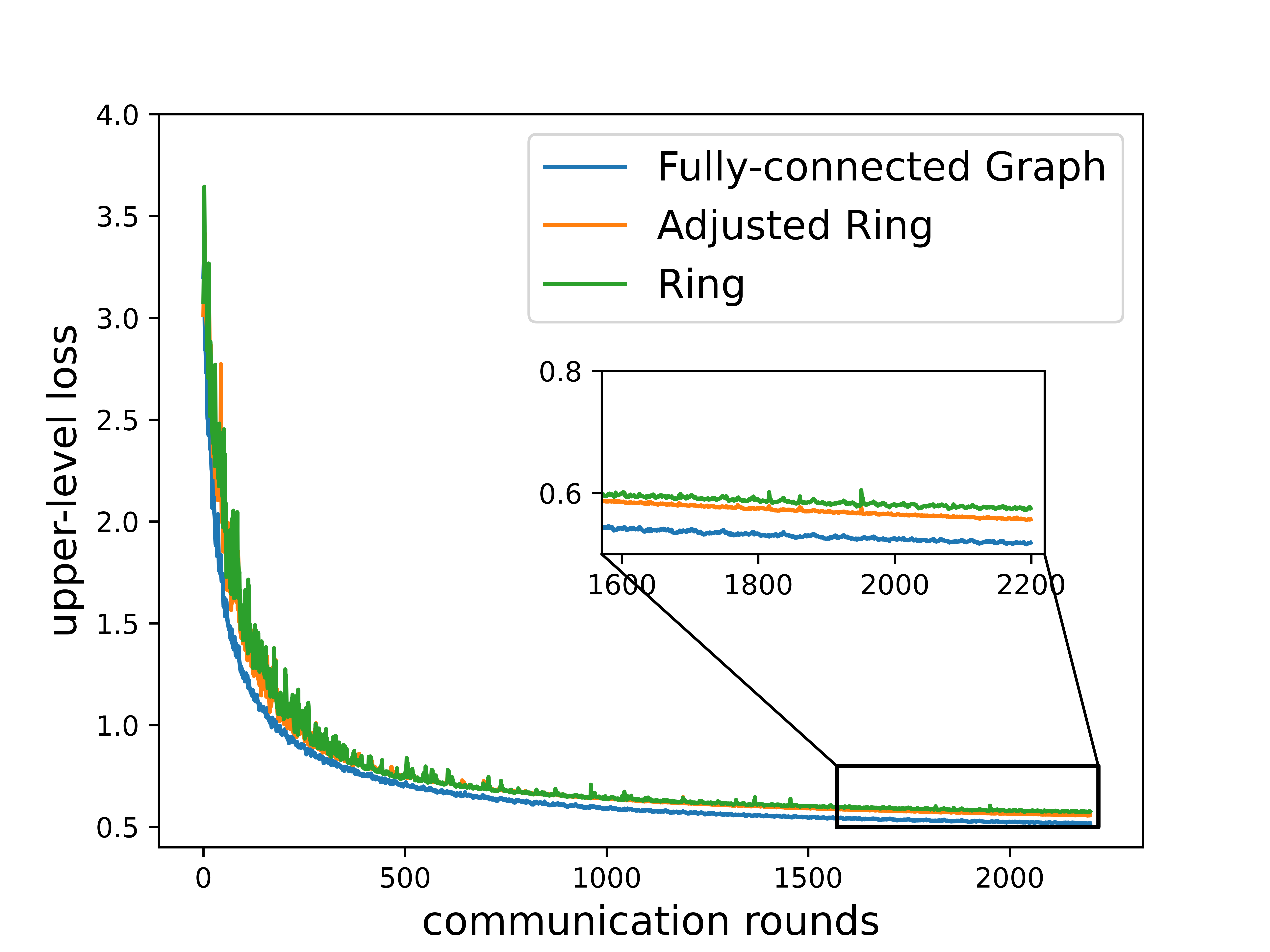
(a) $h=0.80$, upper-level loss

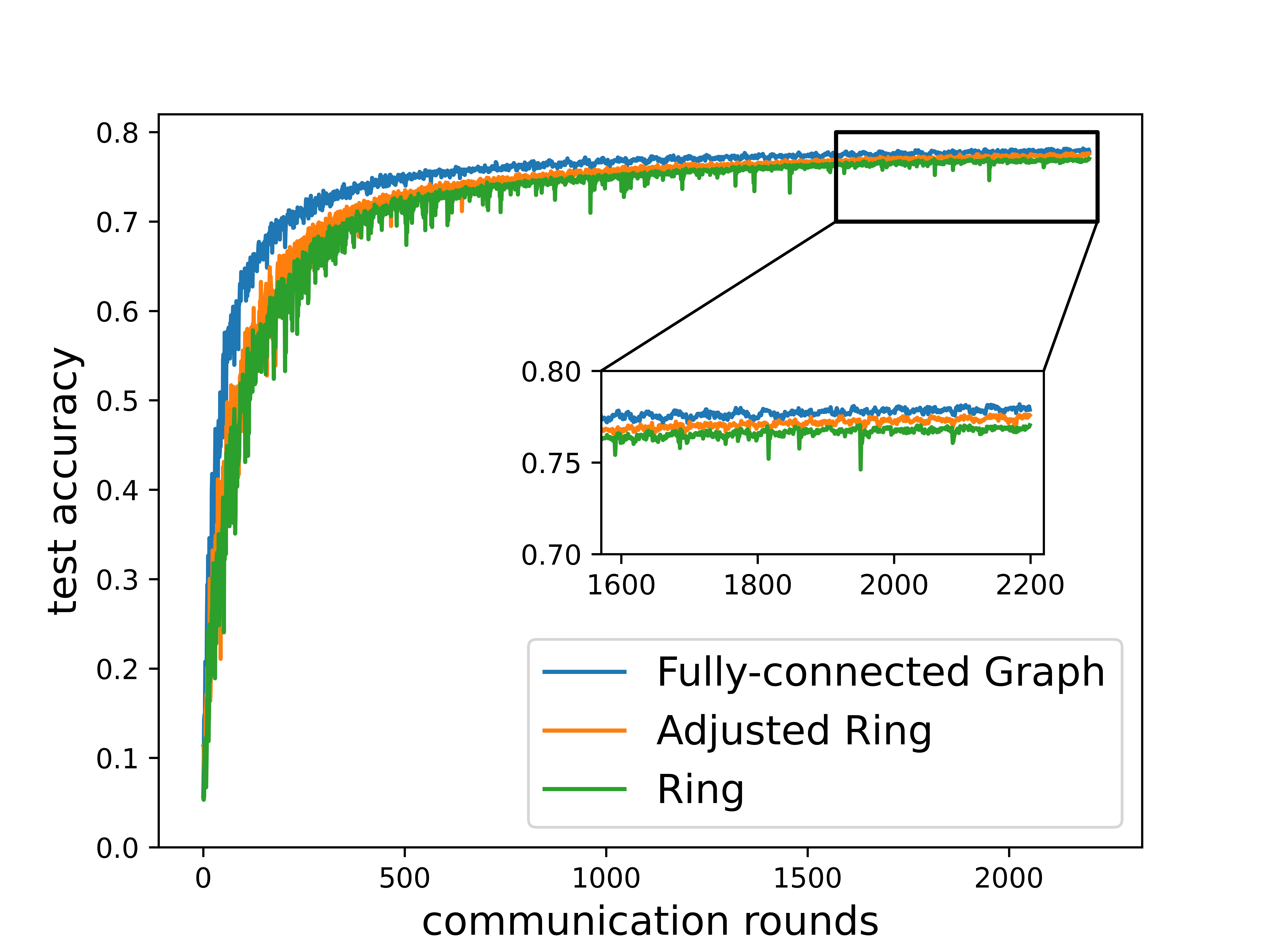
(b) $h=0.80$, test accuracy

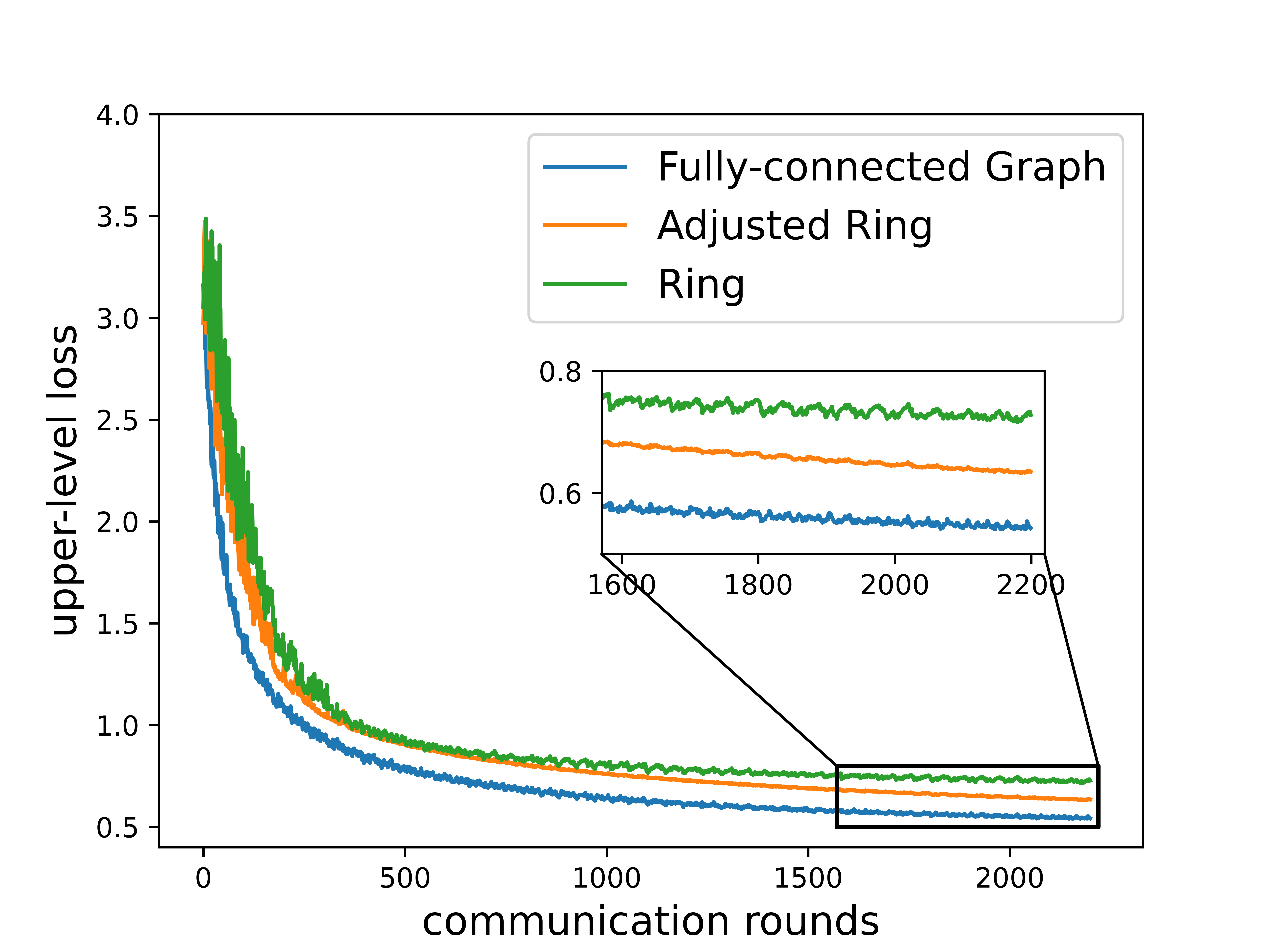
(c) $h=0.95$, upper-level loss

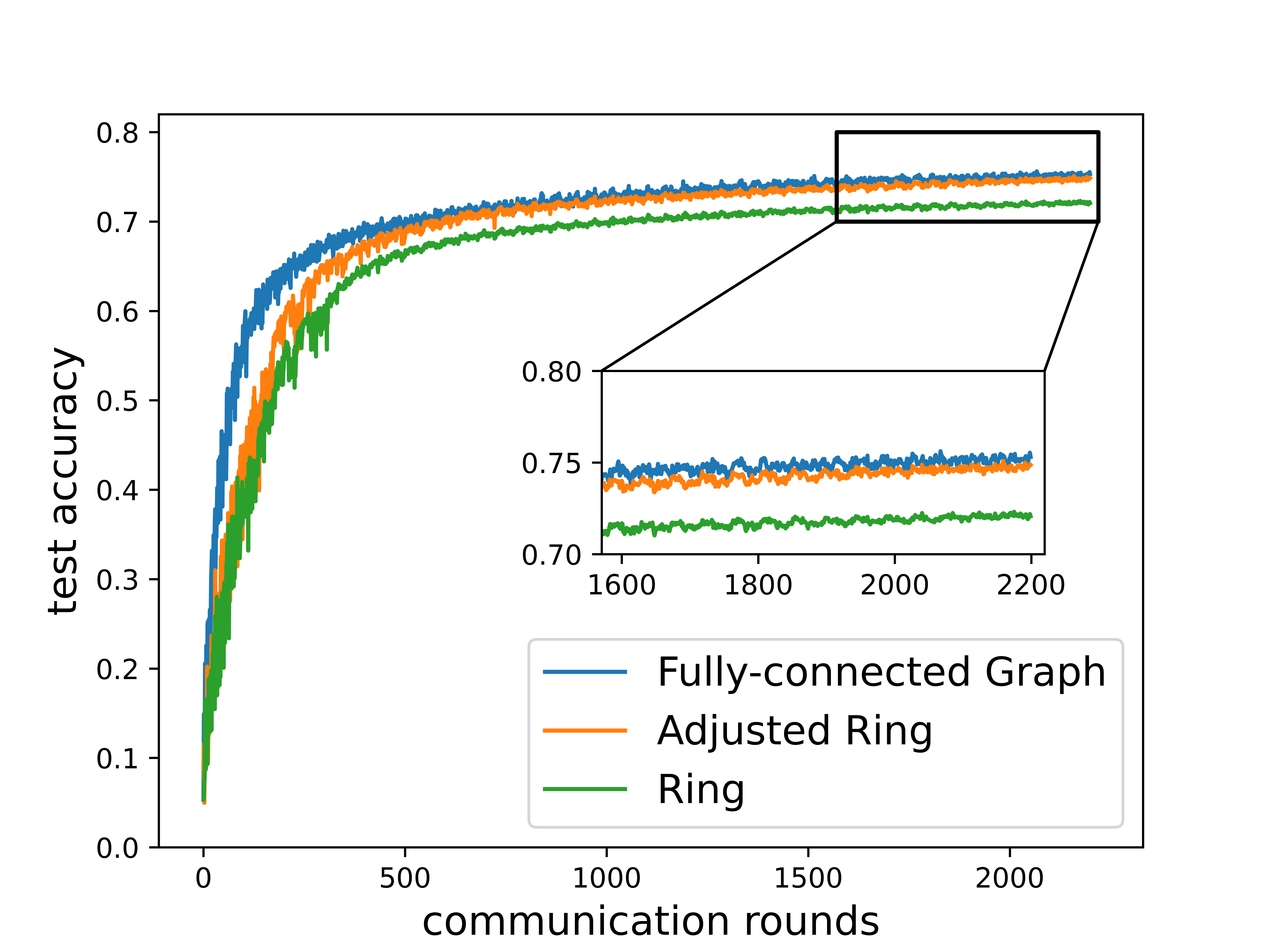
(d) $h=0.95$, test accuracy

Figure 5: The upper-level loss and test accuracy of D-SOBA with different topologies and data heterogeneity.

C.3 Hyper-cleaning problem for Fashion MNIST dataset

We conduct the proposed D-SOBA, MA-DSBO, and Gossip DSBO to a data hyper-clean problem [50] for a Fashion MNIST dataset [58], which consists of 60000 images for training and 10000 images for testing. Then we split the 60000 training images into the training set and validation set, which contains 50000 images and 10000 images separately.

In the data hyper-clean problem, we aim to train a classifier in a corrupted setting in which the label of each training data is replaced by a random class number with a probability $p$ (i.e. the corruption rate) on a decentralized network with $N=10$ clients. It can be viewed as a bilevel optimization problem (1) whose loss functions on the upper and lower level of the $i$-th node denote:

$$f_{i}(x,y) =\dfrac{1}{\left|\mathcal{D}_{val}^{(i)}\right|}\sum_{(\xi_{e},\zeta_{e})\in D_{val}^{(i)}}L(\phi(\xi_{e};y),\zeta_{e}),$$ (122a)

$$g_{i}(x,y) =\dfrac{1}{\left|\mathcal{D}_{tr}^{(i)}\right|}\sum_{(\xi_{e},\zeta_{e})\in\mathcal{D}_{tr}^{(i)}}\sigma(x_{e})L(\phi(\xi_{e};y),\zeta_{e})+C\left\|y\right\|^{2},$$ (122b)

where $\phi$ denotes the parameters of a two-layer MLP network with a 300-dim hidden layer and ReLU activation while $y$ denotes its parameters. $L$ denotes cross-entropy loss, $\sigma(u)=(1+e^{-u})^{-1}$ denotes the sigmoid function. $\mathcal{D}_{val}^{(i)}$ and $\mathcal{D}_{tr}^{(i)}$ denote the validation and training sets of the $i$-th client, which are sampled randomly by Dirichlet distribution with parameters $(\alpha_{1},\cdots,\alpha_{N-1})=(0.1,\cdots,0.1)$ in non-i.i.d. cases [37]. Following with the setting in [50], we set $C=0.001$.

We firstly use D-SOBA, MA-DSBO, and Gossip DSBO to solve (122) with different $p$ over an exponential graph [64]. For all three algorithms, the step-size are set to 0.1 and the batch size are set to 200. Meanwhile, the momentum terms of D-SOBA and MA-DSBO are set to 0.2. For MA-DSBO, we set the number of inner-loop iterations $T=5$ and the number of outer-loop iterations $K=5$. For Gossip DSBO, we set the number of Hessian-inverse estimation iterations $T=5$. At the end of the update of outer parameters, we use the average of $y$ among all clients to do the classification of the test set. The result has been shown in Section 4.

Then we conduct the D-SOBA with different topologies including Adjusted Ring, 2D-Torus, Exponential group as well as the centralized case in the non-i.i.d setting. We set $p=0.2$, and repeat all the cases 10 times and illustrate the mean of all trials. Figure 6 illustrates the upper-level loss and test accuracy of different cases, from which we can observe that a topology with a small spectral gap can converge fast and reach a high test accuracy in a shorter time.

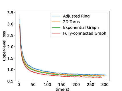
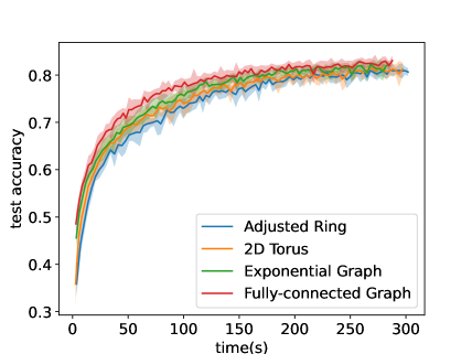
Figure 6: The upper-level loss and test accuracy of D-SOBA and MA-DSBO with different communication topologies.

References

- [1] Sulaiman A Alghunaim and Kun Yuan. A unified and refined convergence analysis for non-convex decentralized learning. IEEE Transactions on Signal Processing, 2022.
- [2] Sanjeev Arora, Simon Du, Sham Kakade, Yuping Luo, and Nikunj Saunshi. Provable representation learning for imitation learning via bi-level optimization. In International Conference on Machine Learning, pages 367–376. PMLR, 2020.
- [3] Mahmoud Assran, Nicolas Loizou, Nicolas Ballas, and Mike Rabbat. Stochastic gradient push for distributed deep learning. In International Conference on Machine Learning (ICML), pages 344–353, 2019.
- [4] L Bertinetto, J Henriques, P Torr, and A Vedaldi. Meta-learning with differentiable closed-form solvers. In International Conference on Learning Representations (ICLR), 2019. International Conference on Learning Representations, 2019.
- [5] Zalán Borsos, Mojmir Mutny, and Andreas Krause. Coresets via bilevel optimization for continual learning and streaming. Advances in neural information processing systems, 33:14879–14890, 2020.
- [6] Jerome Bracken and James T McGill. Mathematical programs with optimization problems in the constraints. Operations research, 21(1):37–44, 1973.
- [7] Tsung-Hui Chang, Mingyi Hong, and Xiangfeng Wang. Multi-agent distributed optimization via inexact consensus admm. IEEE Transactions on Signal Processing, 63(2):482–497, 2014.
- [8] Jianshu Chen and Ali H Sayed. Diffusion adaptation strategies for distributed optimization and learning over networks. IEEE Transactions on Signal Processing, 60(8):4289–4305, 2012.
- [9] Tianyi Chen, Yuejiao Sun, Quan Xiao, and Wotao Yin. A single-timescale method for stochastic bilevel optimization. In International Conference on Artificial Intelligence and Statistics, pages 2466–2488. PMLR, 2022.
- [10] Tianyi Chen, Yuejiao Sun, and Wotao Yin. Closing the gap: Tighter analysis of alternating stochastic gradient methods for bilevel problems. Advances in Neural Information Processing Systems, 34:25294–25307, 2021.
- [11] Xuxing Chen, Minhui Huang, and Shiqian Ma. Decentralized bilevel optimization. arXiv preprint arXiv:2206.05670, 2022.
- [12] Xuxing Chen, Minhui Huang, Shiqian Ma, and Krishna Balasubramanian. Decentralized stochastic bilevel optimization with improved per-iteration complexity. In International Conference on Machine Learning, pages 4641–4671. PMLR, 2023.
- [13] Xuxing Chen, Tesi Xiao, and Krishnakumar Balasubramanian. Optimal algorithms for stochastic bilevel optimization under relaxed smoothness conditions. arXiv preprint arXiv:2306.12067, 2023.
- [14] Yiming Chen, Kun Yuan, Yingya Zhang, Pan Pan, Yinghui Xu, and Wotao Yin. Accelerating gossip sgd with periodic global averaging. In International Conference on Machine Learning (ICML), 2021.
- [15] Ashok Cutkosky and Francesco Orabona. Momentum-based variance reduction in non-convex sgd. Advances in neural information processing systems, 32, 2019.
- [16] Mathieu Dagréou, Pierre Ablin, Samuel Vaiter, and Thomas Moreau. A framework for bilevel optimization that enables stochastic and global variance reduction algorithms. Advances in Neural Information Processing Systems, 35:26698–26710, 2022.
- [17] P. Di Lorenzo and G. Scutari. Next: In-network nonconvex optimization. IEEE Transactions on Signal and Information Processing over Networks, 2(2):120–136, 2016.
- [18] Justin Domke. Generic methods for optimization-based modeling. In Artificial Intelligence and Statistics, pages 318–326. PMLR, 2012.
- [19] Youran Dong, Shiqian Ma, Junfeng Yang, and Chao Yin. A single-loop algorithm for decentralized bilevel optimization. arXiv preprint arXiv:2311.08945, 2023.
- [20] John C Duchi, Alekh Agarwal, and Martin J Wainwright. Dual averaging for distributed optimization: Convergence analysis and network scaling. IEEE Transactions on Automatic control, 57(3):592–606, 2011.
- [21] Luca Franceschi, Paolo Frasconi, Saverio Salzo, Riccardo Grazzi, and Massimiliano Pontil. Bilevel programming for hyperparameter optimization and meta-learning. In International conference on machine learning, pages 1568–1577. PMLR, 2018.
- [22] Hongchang Gao, Bin Gu, and My T Thai. On the convergence of distributed stochastic bilevel optimization algorithms over a network. In International Conference on Artificial Intelligence and Statistics, pages 9238–9281. PMLR, 2023.
- [23] Saeed Ghadimi and Mengdi Wang. Approximation methods for bilevel programming. arXiv preprint arXiv:1802.02246, 2018.
- [24] Andrew Gibiansky. Bringing HPC techniques to deep learning. https://andrew.gibiansky.com/blog/machine-learning/baidu-allreduce/, 2017. Accessed: 2020-08-12.
- [25] Riccardo Grazzi, Luca Franceschi, Massimiliano Pontil, and Saverio Salzo. On the iteration complexity of hypergradient computation. In International Conference on Machine Learning, pages 3748–3758. PMLR, 2020.
- [26] Andreas Griewank and Andrea Walther. Evaluating derivatives: principles and techniques of algorithmic differentiation. SIAM, 2008.
- [27] Zhishuai Guo, Quanqi Hu, Lijun Zhang, and Tianbao Yang. Randomized stochastic variance-reduced methods for multi-task stochastic bilevel optimization. arXiv preprint arXiv:2105.02266, 2021.
- [28] Mingyi Hong, Hoi-To Wai, Zhaoran Wang, and Zhuoran Yang. A two-timescale stochastic algorithm framework for bilevel optimization: Complexity analysis and application to actor-critic. SIAM Journal on Optimization, 33(1):147–180, 2023.
- [29] Minhui Huang, Dewei Zhang, and Kaiyi Ji. Achieving linear speedup in non-iid federated bilevel learning. arXiv preprint arXiv:2302.05412, 2023.
- [30] Kaiyi Ji, Junjie Yang, and Yingbin Liang. Bilevel optimization: Convergence analysis and enhanced design. In International conference on machine learning, pages 4882–4892. PMLR, 2021.
- [31] Rie Johnson and Tong Zhang. Accelerating stochastic gradient descent using predictive variance reduction. Advances in neural information processing systems, 26, 2013.
- [32] Anastasia Koloskova, Nicolas Loizou, Sadra Boreiri, Martin Jaggi, and Sebastian U Stich. A unified theory of decentralized sgd with changing topology and local updates. In International Conference on Machine Learning (ICML), pages 1–12, 2020.
- [33] Mu Li, David G Andersen, Jun Woo Park, Alexander J Smola, Amr Ahmed, Vanja Josifovski, James Long, Eugene J Shekita, and Bor-Yiing Su. Scaling distributed machine learning with the parameter server. In 11th USENIX Symposium on Operating Systems Design and Implementation (OSDI 14), pages 583–598, 2014.
- [34] Z. Li, W. Shi, and M. Yan. A decentralized proximal-gradient method with network independent step-sizes and separated convergence rates. IEEE Transactions on Signal Processing, July 2019. early acces. Also available on arXiv:1704.07807.
- [35] Xiangru Lian, Ce Zhang, Huan Zhang, Cho-Jui Hsieh, Wei Zhang, and Ji Liu. Can decentralized algorithms outperform centralized algorithms? A case study for decentralized parallel stochastic gradient descent. In Advances in Neural Information Processing Systems, pages 5330–5340, 2017.
- [36] Xiangru Lian, Ce Zhang, Huan Zhang, Cho-Jui Hsieh, Wei Zhang, and Ji Liu. Can decentralized algorithms outperform centralized algorithms? a case study for decentralized parallel stochastic gradient descent. In I. Guyon, U. Von Luxburg, S. Bengio, H. Wallach, R. Fergus, S. Vishwanathan, and R. Garnett, editors, Advances in Neural Information Processing Systems, volume 30. Curran Associates, Inc., 2017.
- [37] Tao Lin, Sai Praneeth Karimireddy, Sebastian U Stich, and Martin Jaggi. Quasi-global momentum: Accelerating decentralized deep learning on heterogeneous data. In International Conference on Machine Learning, 2021.
- [38] Zhuqing Liu, Xin Zhang, Prashant Khanduri, Songtao Lu, and Jia Liu. Interact: Achieving low sample and communication complexities in decentralized bilevel learning over networks. In Proceedings of the Twenty-Third International Symposium on Theory, Algorithmic Foundations, and Protocol Design for Mobile Networks and Mobile Computing, pages 61–70, 2022.
- [39] Songtao Lu, Xiaodong Cui, Mark S Squillante, Brian Kingsbury, and Lior Horesh. Decentralized bilevel optimization for personalized client learning. In ICASSP 2022-2022 IEEE International Conference on Acoustics, Speech and Signal Processing (ICASSP), pages 5543–5547. IEEE, 2022.
- [40] Songtao Lu, Siliang Zeng, Xiaodong Cui, Mark Squillante, Lior Horesh, Brian Kingsbury, Jia Liu, and Mingyi Hong. A stochastic linearized augmented lagrangian method for decentralized bilevel optimization. Advances in Neural Information Processing Systems, 35:30638–30650, 2022.
- [41] Songtao Lu, Xinwei Zhang, Haoran Sun, and Mingyi Hong. Gnsd: A gradient-tracking based nonconvex stochastic algorithm for decentralized optimization. In 2019 IEEE Data Science Workshop (DSW), pages 315–321. IEEE, 2019.
- [42] Yucheng Lu and Christopher De Sa. Optimal complexity in decentralized training. In International Conference on Machine Learning, pages 7111–7123. PMLR, 2021.
- [43] Dougal Maclaurin, David Duvenaud, and Ryan Adams. Gradient-based hyperparameter optimization through reversible learning. In International conference on machine learning, pages 2113–2122. PMLR, 2015.
- [44] Angelia Nedić and Alex Olshevsky. Distributed optimization over time-varying directed graphs. IEEE Transactions on Automatic Control, 60(3):601–615, 2014.
- [45] A. Nedic, A. Olshevsky, and W. Shi. Achieving geometric convergence for distributed optimization over time-varying graphs. SIAM Journal on Optimization, 27(4):2597–2633, 2017.
- [46] Angelia Nedic and Asuman Ozdaglar. Distributed subgradient methods for multi-agent optimization. IEEE Transactions on Automatic Control, 54(1):48–61, 2009.
- [47] Youcheng Niu, Jinming Xu, Ying Sun, Yan Huang, and Li Chai. Distributed stochastic bilevel optimization: Improved complexity and heterogeneity analysis. arXiv preprint arXiv:2312.14690, 2023.
- [48] Shi Pu, Alex Olshevsky, and Ioannis Ch Paschalidis. A sharp estimate on the transient time of distributed stochastic gradient descent. IEEE Transactions on Automatic Control, 67(11):5900–5915, 2021.
- [49] Mark Schmidt, Nicolas Le Roux, and Francis Bach. Minimizing finite sums with the stochastic average gradient. Mathematical Programming, 162:83–112, 2017.
- [50] Amirreza Shaban, Ching-An Cheng, Nathan Hatch, and Byron Boots. Truncated back-propagation for bilevel optimization. In The 22nd International Conference on Artificial Intelligence and Statistics, pages 1723–1732. PMLR, 2019.
- [51] W. Shi, Q. Ling, G. Wu, and W. Yin. EXTRA: An exact first-order algorithm for decentralized consensus optimization. SIAM Journal on Optimization, 25(2):944–966, 2015.
- [52] Wei Shi, Qing Ling, Kun Yuan, Gang Wu, and Wotao Yin. On the linear convergence of the admm in decentralized consensus optimization. IEEE Transactions on Signal Processing, 62(7):1750–1761, 2014.
- [53] Alexander Smola and Shravan Narayanamurthy. An architecture for parallel topic models. Proceedings of the VLDB Endowment, 3(1-2):703–710, 2010.
- [54] Jake Snell, Kevin Swersky, and Richard Zemel. Prototypical networks for few-shot learning. Advances in neural information processing systems, 30, 2017.
- [55] Hanlin Tang, Xiangru Lian, Ming Yan, Ce Zhang, and Ji Liu. : Decentralized training over decentralized data. In International Conference on Machine Learning, pages 4848–4856, 2018.
- [56] Davoud Ataee Tarzanagh, Mingchen Li, Christos Thrampoulidis, and Samet Oymak. Fednest: Federated bilevel, minimax, and compositional optimization. In International Conference on Machine Learning, pages 21146–21179. PMLR, 2022.
- [57] Luis N Vicente and Paul H Calamai. Bilevel and multilevel programming: A bibliography review. Journal of Global optimization, 5(3):291–306, 1994.
- [58] Han Xiao, Kashif Rasul, and Roland Vollgraf. Fashion-mnist: a novel image dataset for benchmarking machine learning algorithms. arXiv preprint arXiv:1708.07747, 2017.
- [59] Ran Xin, Usman A Khan, and Soummya Kar. An improved convergence analysis for decentralized online stochastic non-convex optimization. arXiv preprint arXiv:2008.04195, 2020.
- [60] J. Xu, S. Zhu, Y. C. Soh, and L. Xie. Augmented distributed gradient methods for multi-agent optimization under uncoordinated constant stepsizes. In IEEE Conference on Decision and Control (CDC), pages 2055–2060, Osaka, Japan, 2015.
- [61] Junjie Yang, Kaiyi Ji, and Yingbin Liang. Provably faster algorithms for bilevel optimization. Advances in Neural Information Processing Systems, 34:13670–13682, 2021.
- [62] Shuoguang Yang, Xuezhou Zhang, and Mengdi Wang. Decentralized gossip-based stochastic bilevel optimization over communication networks. Advances in Neural Information Processing Systems, 35:238–252, 2022.
- [63] Yifan Yang, Peiyao Xiao, and Kaiyi Ji. Simfbo: Towards simple, flexible and communication-efficient federated bilevel learning. arXiv preprint arXiv:2305.19442, 2023.
- [64] Bicheng Ying, Kun Yuan, Yiming Chen, Hanbin Hu, Pan Pan, and Wotao Yin. Exponential graph is provably efficient for decentralized deep training. In Advances in Neural Information Processing Systems (NeurIPS), 2021.
- [65] Bicheng Ying, Kun Yuan, Hanbin Hu, Yiming Chen, and Wotao Yin. Bluefog: Make decentralized algorithms practical for optimization and deep learning. arXiv preprint arXiv:2111.04287, 2021.
- [66] Kun Yuan, Sulaiman A Alghunaim, and Xinmeng Huang. Removing data heterogeneity influence enhances network topology dependence of decentralized SGD. Journal of Machine Learning Research, 24(280):1–53, 2023.
- [67] Kun Yuan, Yiming Chen, Xinmeng Huang, Yingya Zhang, Pan Pan, Yinghui Xu, and Wotao Yin. DecentLaM: Decentralized momentum SGD for large-batch deep training. International Conference on Computer Vision, 2021.
- [68] Kun Yuan, Xinmeng Huang, Yiming Chen, Xiaohan Zhang, Yingya Zhang, and Pan Pan. Revisiting optimal convergence rate for smooth and non-convex stochastic decentralized optimization. Advances in Neural Information Processing Systems, 35:36382–36395, 2022.
- [69] Kun Yuan, Qing Ling, and Wotao Yin. On the convergence of decentralized gradient descent. SIAM Journal on Optimization, 26(3):1835–1854, 2016.
- [70] K. Yuan, B. Ying, X. Zhao, and A. H. Sayed. Exact dffusion for distributed optimization and learning – Part I: Algorithm development. IEEE Transactions on Signal Processing, 67(3):708 – 723, 2019.
- [71] Yihua Zhang, Prashant Khanduri, Ioannis Tsaknakis, Yuguang Yao, Mingyi Hong, and Sijia Liu. An introduction to bi-level optimization: Foundations and applications in signal processing and machine learning. arXiv preprint arXiv:2308.00788, 2023.
- [72] Yihan Zhang, My T Thai, Jie Wu, and Hongchang Gao. On the communication complexity of decentralized bilevel optimization. arXiv preprint arXiv:2311.11342, 2023.
- [73] Yihua Zhang, Guanhua Zhang, Prashant Khanduri, Mingyi Hong, Shiyu Chang, and Sijia Liu. Revisiting and advancing fast adversarial training through the lens of bi-level optimization. In International Conference on Machine Learning, pages 26693–26712. PMLR, 2022.