Risk-Aware MPC for Stochastic Systems with Runtime Temporal Logics

Abstract

: This paper concerns the risk-aware control of stochastic systems with temporal logic specifications dynamically assigned during runtime. Conventional risk-aware control typically assumes that all specifications are predefined and remain unchanged during runtime. In this paper, we propose a novel, provably correct control scheme for linear systems with unbounded stochastic disturbances that dynamically evaluates the feasibility of runtime signal temporal logic specifications and automatically reschedules the control inputs. The method guarantees the probabilistic satisfaction of newly accepted runtime specifications without sacrificing the satisfaction of the previously accepted ones. The proposed control method is validated by a robotic motion planning case study. The idea of closed-loop control rescheduling with probabi-listic risk guarantees provides a novel solution for runtime control synthesis of stochastic systems.

1 introduction

Practical engineering systems are required to accomplish certain desired tasks with restricted risk levels. This can be achieved by risk-aware control incorporating stochastic uncertainties, which renders a stochastic planning problem with probabilistic risk constraints (Sadigh and Kapoor, 2015). For stochastic systems with signal temporal logic (STL) specifications, control synthesis has been performed in (Farahani et al., 2017) by underapproximating the fixed chance constraints using linear inequalities. Similarly, for dynamic systems with bounded disturbances, control synthesis has been performed based on the worst-case optimization (Farahani et al., 2015; Raman et al., 2015; Sadraddini and Belta, 2019). For probability STL (PrSTL), one can convert the probabilistic satisfaction of specifications to a Boolean combination of risk constraints (Sadigh and Kapoor, 2016). For example, this method has been used in (Mehr et al., 2017) to solve the ramp merging problem.

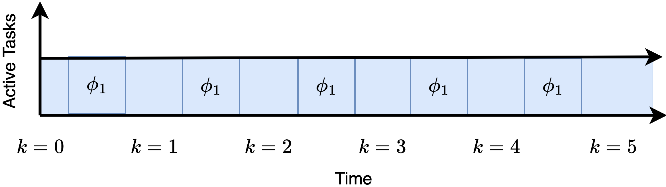
Figure 1: An illustration of the classical fixed specification problem.

Common amongst all previously mentioned works is the assumption of predefined specifications, as illustrated in Fig. 1. Moreover, predefining specifications extends to most work on conventional risk-aware control of stochastic systems. Nevertheless, practical applications in multi-robot systems and human-robot collaboration often need to dynamically allocate tasks during runtime (Zhu and Yang, 2006; Bruno and Antonelli, 2018). For example, a restaurant service robot delivering a dish may receive another delivery task at any time. It then needs to evaluate whether taking the order affects the accomplishment of the current delivery. As shown in Fig. 2, for a general control system, this indicates that it should automatically reschedule its current control policy by evaluating the risks of newly assigned specifications during runtime. To our knowledge, such control schemes have yet to be introduced in the literature, although some inspiring work exists. A shrinking-horizon model predictive control (MPC) method has been provided in (Farahani et al., 2018) to solve closed-loop risk-aware control of stochastic systems with temporal logic specifications. In (Mustafa et al., 2023), multiple risk bounds are evaluated from a set of control policies where the best policy with the least conservativeness is selected. The work in (Farahani et al., 2015) proposes a scheme to accept or reject a specification by evaluating its feasibility. In (Hewing and Zeilinger, 2018), tube-based stochastic MPC has been used to synthesize controllers for predefined probabilistic set constraints. In (Engelaar et al., 2023), probabilistic reachable tubes have been used to optimize risk bounds over predefined probabilistic set constraints. These approaches and concepts provide inspiring ideas for the risk re-evaluation and control rescheduling of stochastic systems with runtime specifications.

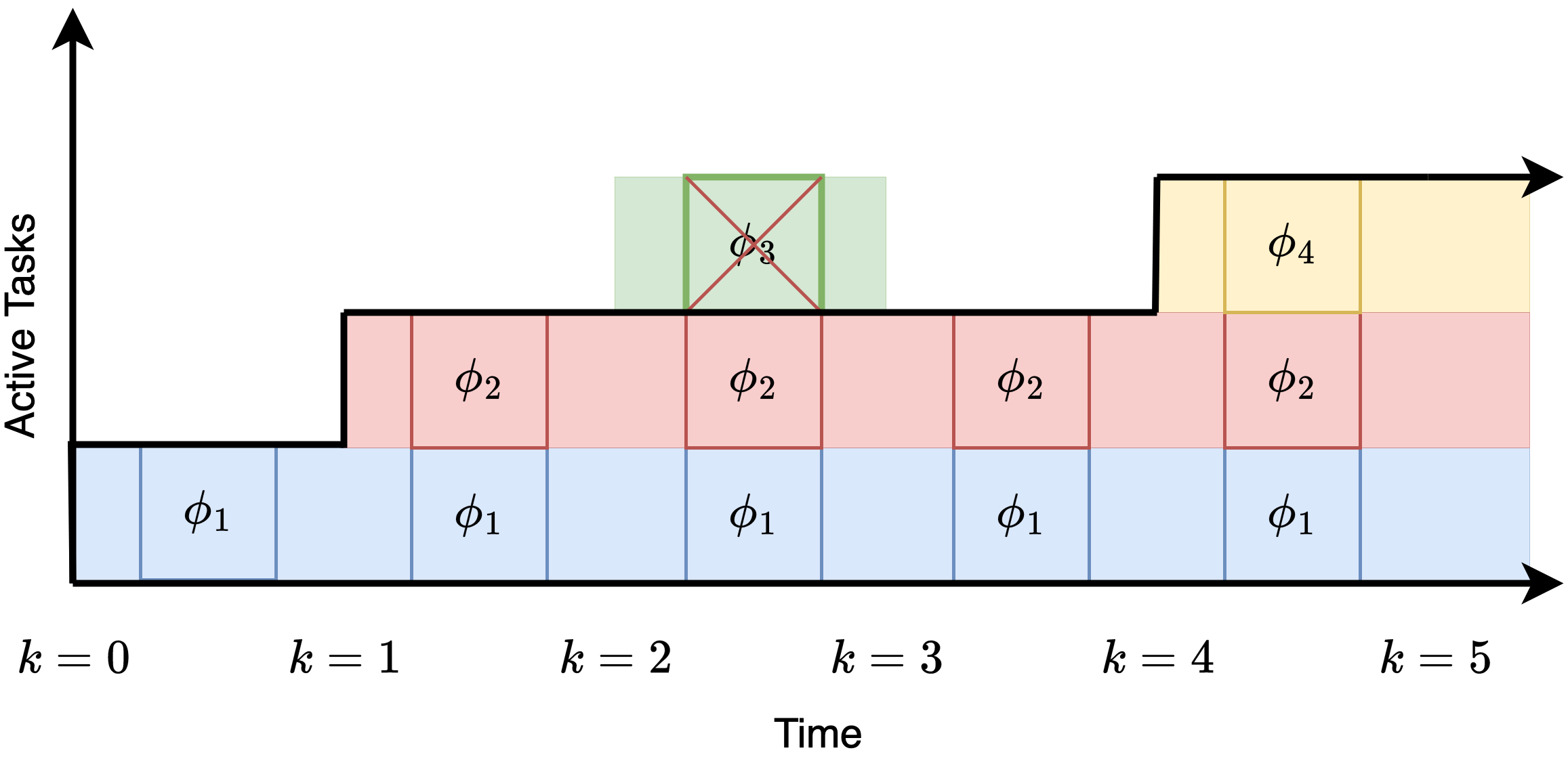
Figure 2: An illustration of the dynamic specification problem. Here, a new task is accepted at times $k=0$, $k=1$, and $k=4$, while at time $k=2$, a task is rejected.

Motivated by the above open problem, this paper develops a risk-aware rescheduling control scheme for linear systems with runtime STL specifications and unbounded disturbance. Inspired by the shrinking horizon MPC approach of (Farahani et al., 2018), we design a closed-loop control method by solving a stochastic planning problem with probabilistic tube-based constraints (Hewing and Zeilinger, 2018) at each time, with historical system trajectories kept fixed. Once an STL specification is assigned during runtime, we use probabilistic reachable tubes (Engelaar et al., 2023) to re-calculate the risk bounds of the probabilistic constraints and reschedule the control input to satisfy the newly assigned specifications while retaining the satisfaction of the previously assigned specifications. The developed algorithm rejects any assigned specification that might compromise previously accepted specifications. A two-dimensional vehicle motion planning case with dynamically assigned targets is used to validate the efficacy of our method.

The remaining part of the paper is organized as follows. In Sec. 2, the preliminaries, system dynamics, temporal specifications, probability satisfaction, and problem statement are introduced. Sec. 3 explains the control design based on probabilistic guarantee computation for STL specifications and the control rescheduling for newly assigned specifications. In Sec. 4, a robot motion planning case is used to validate the proposed method. Finally, Sec. 5 concludes the paper.

2 Preliminaries and Problem Statement

This section introduces the preliminaries, class of systems, temporal logics, and basic assumptions, culminating in a problem statement and an approach.

2.1 Preliminaries

For a given probability measure $\mathbb{P}$ defined over Borel measurable space $(\mathbb{X},\mathcal{B}(\mathbb{X}))$, we denote the probability of an event $\mathcal{A}\in\mathcal{B}(\mathbb{X})$ as $\mathbb{P}(\mathcal{A})$. In this paper, we will work with Euclidean spaces and Borel measurability. Further details on measurability are omitted, and we refer the interested reader to (Bertsekas and Shreve, 1996). Additionally, any half-space $H\subset\mathbb{R}^{n}$ is defined as $H:=\{x\in\mathbb{R}^{n}\mid g^{T}x\geq b\}$ with $g\in\mathbb{R}^{n}$ and $b\in\mathbb{R}$. A polyhedron is the intersection of finitely many half-spaces, also denoted as $H:=\{x\in\mathbb{R}^{n}\mid Gx\geq b\}$ with $G\in\mathbb{R}^{q\times n}$ and $b\in\mathbb{R}^{q}$. The 2-norm is defined by $||x||=\sqrt{x^{T}x}$ with $x\in\mathbb{R}^{n}$. The identity matrix is denoted by $I_{n}\in\mathbb{R}^{n\times n}$. The vector of all elements one is denoted by $\boldsymbol{1}_{n}\in\mathbb{R}^{n}$, but if the context is clear, it will instead be denoted by $\boldsymbol{1}$. The zero vector is denoted by $\boldsymbol{0}_{n}\in\mathbb{R}^{n}$, but if the context is clear, it will instead be denoted by $0$.

2.2 Class of Systems

In this paper, we consider systems with linear time-invariant dynamics with additive noise, given by

$$x(k+1)=Ax(k)+Bu(k)+w(k),$$ (1)

where matrix pair $(A,B)$ is stabilizable, $x\in\mathbb{X}\subseteq\mathbb{R}^{n}$ is the state of the system, $x(0)\in\mathbb{X}$ is an initial state, $u\in\mathbb{U}\subseteq\mathbb{R}^{m}$ is the input of the system and $w\in\mathbb{R}^{n}$ is an independent, identically distributed noise disturbance with distribution $\mathcal{Q}_{w}$, i.e., $w(k)\sim\mathcal{Q}_{w}$, which can have infinite support. We will assume that the distribution has at least a known mean and variance, with the latter assumed to be strictly positive definite. Additionally, we assume that the distribution is central convex unimodal.

To control the system, we define a sequence of policies $\boldsymbol{f}:=\{f_{0},f_{1},\dots\}$, such that $f_{k}:\mathbb{H}_{k}\to\mathbb{U}$ maps the history of states and inputs to inputs, i.e., $\mathbb{H}_{k}:=(\mathbb{X}\times\mathbb{U})^{k}\times\mathbb{X}$ with element $(x(0),u(0),\cdots,u(k-1),x(k))$. By implementing controller $\boldsymbol{f}$ upon system (1), we obtain its controlled form for which the control input satisfies the feedback law $u(k)=f_{k}(h(k))$ with $h(k)\in\mathbb{H}_{k}$. We indicate the input sequence of system (1) by $\boldsymbol{u}:=\{u(0),u(1),\dots\}$ and define its executions as sequences of states $\boldsymbol{x}:=\{x(0),x(1),\dots\}$, referred to as signals. Any signal $\boldsymbol{x}$ can be interpreted as a realization of the probability distribution induced by implementing controller $\boldsymbol{f}$, denoted by $\boldsymbol{x}\sim\mathbb{P}_{\boldsymbol{f}}$. Similarly, the suffix fragment $\vec{\boldsymbol{x}}_{k}=\{x(k),x(k+1),\dots\}$ of a signal $\boldsymbol{x}$ can be interpreted as a realization $\boldsymbol{\vec{x}}_{k}\sim\mathbb{P}_{\boldsymbol{f},k}$. We define the segment of any signal $\boldsymbol{x}:=\{x(0),x(1),\ldots\}$ by $\boldsymbol{x}_{[i,j]}:=\{x(i),\ldots,x(j)\}$ with $i\leq j$.

2.3 Signal Temporal Logic

To mathematically describe tasks, e.g., reaching a target space within a given time frame, we consider specifications given by signal temporal logic. Here, we assume that all STL specifications adhere to the negation normal form (NNF), see (Raman et al., 2014). This assumption does not restrict the overall framework since (Sadraddini and Belta, 2015) proves that every STL specification can be rewritten into the negation normal form.

STL consists of predicates $\mu$ that are either true ($\top$) or false ($\bot$). Each predicate $\mu$ is described by a function $h:\mathbb{R}^{n}\to\mathbb{R}^{q}$ as follows

$$\mu:=\begin{cases}\top\text{ if }h(x)\geq 0\\ \bot\text{ if }h(x)<0.\end{cases}$$ (2)

Note that $x$ in $h(x)$ is a vector, not a signal. Let $\boldsymbol{x}(k)\in\mathbb{R}^{n}$ denote the $k$-th element of signal $\boldsymbol{x}$, then $h(\boldsymbol{x}(k))$ determines the truth value of $\mu$ at time $k$. We will assume that all predicate functions are linear affine functions of the form $h(x)=Gx-b$ with $G\in\mathbb{R}^{q\times n}$, $b\in\mathbb{R}^{q}$ and $||g_{j}||=1$ for all $j\in\{1,\cdots,q\}$, where $g_{j}$ is the $j$-th row of $G$. Notice that satisfaction of the predicate $\mu$ is defined by whether $x$ is contained within the polyhedron $H_{\mu}:=\{x\in\mathbb{R}^{n}\mid Gx\geq b\}$. Since all rows of $G$ are normalized, we denote the polyhedron $H_{\mu}$ as normalized.

Let the set of all predicates be given by $\mathcal{P}$. The syntax of STL will be given by

$$\phi::=\top\mid\mu\mid\lnot\mu\mid\phi_{1}\wedge\phi_{2}\mid\phi_{1}\vee\phi_{2}\mid\square_{[a,b]}\phi\mid\phi_{1}\ U_{[a,b]}\ \phi_{2},$$

where $\mu\in\mathcal{P}$, $\phi$, $\phi_{1}$ and $\phi_{2}$ are STL formula, $a,b\in\mathbb{N}$, and $a\leq b$. The semantics are given next, where $\boldsymbol{\vec{x}}_{k}\vDash\phi$ denotes the suffix of signal $\boldsymbol{x}$ satisfying specification $\phi$.

Definition 1

The STL semantics are recursively given by:

$$\boldsymbol{\vec{x}}_{k}\vDash\mu \iff h({\boldsymbol{x}(k)})\geq 0$$

$$\boldsymbol{\vec{x}}_{k}\vDash\lnot\mu \iff h({\boldsymbol{x}(k)})<0$$

$$\boldsymbol{\vec{x}}_{k}\vDash\phi_{1}\wedge\phi_{2} \iff \boldsymbol{\vec{x}}_{k}\vDash\phi_{1}\text{ and }\boldsymbol{x}_{k}\vDash\phi_{2}$$

$$\boldsymbol{\vec{x}}_{k}\vDash\phi_{1}\vee\phi_{2} \iff \boldsymbol{\vec{x}}_{k}\vDash\phi_{1}\text{ or }\boldsymbol{x}_{k}\vDash\phi_{2}$$

$$\boldsymbol{\vec{x}}_{k}\vDash\square_{[a,b]}\ \phi \iff \forall k^{\prime}\in[k+a,k+b]:\boldsymbol{\vec{x}}_{k^{\prime}}\vDash\phi$$

$$\boldsymbol{\vec{x}}_{k}\vDash\phi_{1}\ U_{[a,b]}\ \phi_{2} \iff \exists k_{1}\in[k+a,k+b]:\boldsymbol{\vec{x}}_{k_{1}}\vDash\phi_{2}$$

$$\text{ and }\forall k_{2}\in[k,k_{1}],\ \boldsymbol{\vec{x}}_{k_{2}}\vDash\phi_{1}.$$

Here, we introduced a slight abuse of the notation as $[a,b]$ is used to describe the set of all natural numbers within the real interval $[a,b]$. Additional operators can be derived such as the eventually-operator $\lozenge_{[a,b]}\phi:=\top U_{[a,b]}\phi$.

Since the dynamical system is assumed to behave stochastically, each STL specification can only be satisfied with a certain probability. Should a specification be assigned at time $k$, the probability can be determined based on the state $x(k)$, the controller $\boldsymbol{f}$, and the system dynamics (1). Accordingly, we consider the probability that suffix fragment $\vec{\boldsymbol{x}}_{k}$ satisfies specification $\phi$, given state $x(k)$, denoted by

$$\mathbb{P}_{\boldsymbol{f}}(\phi,k):=\mathbb{P}_{\boldsymbol{f},k}(\vec{\boldsymbol{x}}_{k}\vDash\phi\mid x(k)).$$ (3)

Due to the complexity of STL specifications, in general, $\mathbb{P}_{\boldsymbol{f}}(\phi,k)$ cannot be computed directly. Hence, throughout this paper, we will focus on obtaining a lower bound for the probability satisfaction $\mathbb{P}_{\boldsymbol{f}}(\phi,k)$. Accordingly, these lower bounds will function as guarantees on the probabilistic satisfaction of given specifications.

2.4 Problem Statement

We consider a dynamical system (1) that needs to satisfy a sequence of STL specifications. Specifications will be provided in real-time and are assumed to be unknown until the time of assignment. The paper’s objective is two-fold. Firstly, to design a control synthesis technique that gives probabilistic guarantees, i.e., a lower bound on the probability satisfaction of any STL specification. Secondly, to update the control strategy in real-time whenever a new specification is assigned to the dynamical system.

We formalize the above problem description into two problems. Here, we consider the dynamical system (1) with noise distribution $\mathcal{Q}_{w}$ and state update $x(k)$, at each time step $k\in\mathbb{N}$.

Problem 1: Given a STL specification $\phi$ at time $k$ and a maximal risk $r_{\phi,\max}$, develop a method for the synthesis of a controller $\boldsymbol{f}$ that ensures $\mathbb{P}_{\boldsymbol{f}}(\phi,k)\geq 1-r_{\phi,\max}$.

Problem 2: Given a finite sequence of STL specifications $\boldsymbol{\phi}:=\{\phi_{1},\cdots,\phi_{q}\}$ assigned, respectively, at time instances $\{k_{1},\cdots,k_{q}\}$ with $k_{i}<k_{j}$ for $i<j$, with maximal risk $r_{\phi_{i},\max}$, develop a method for updating controller $\boldsymbol{f}$ at time $k$, such that $\mathbb{P}_{\boldsymbol{f}}(\phi_{i},k_{i})\geq 1-r_{\phi_{i},\max}$ if $k_{i}<k$, and, $\mathbb{P}_{\boldsymbol{f}}(\psi,k)\geq 1-r_{\psi,\max}$ if $\psi$ is a newly assigned specification. Here, we allow specification $\psi$ to be rejected if necessary.

Approach. To solve both problems, we consider the approach in Fig. 3. First, we reformulate STL specifications into deterministic linear constraints. Next, a probabilistic reachable tube (PRT) is fitted inside these linear constraints. Here, the tube can upper bound the risk that states are not contained within the tube. By constraining the risks, a tube-based MPC problem is defined at each time instance, which reschedules the controller, decides whether a new specification can be accepted and updates all probabilistic guarantees.

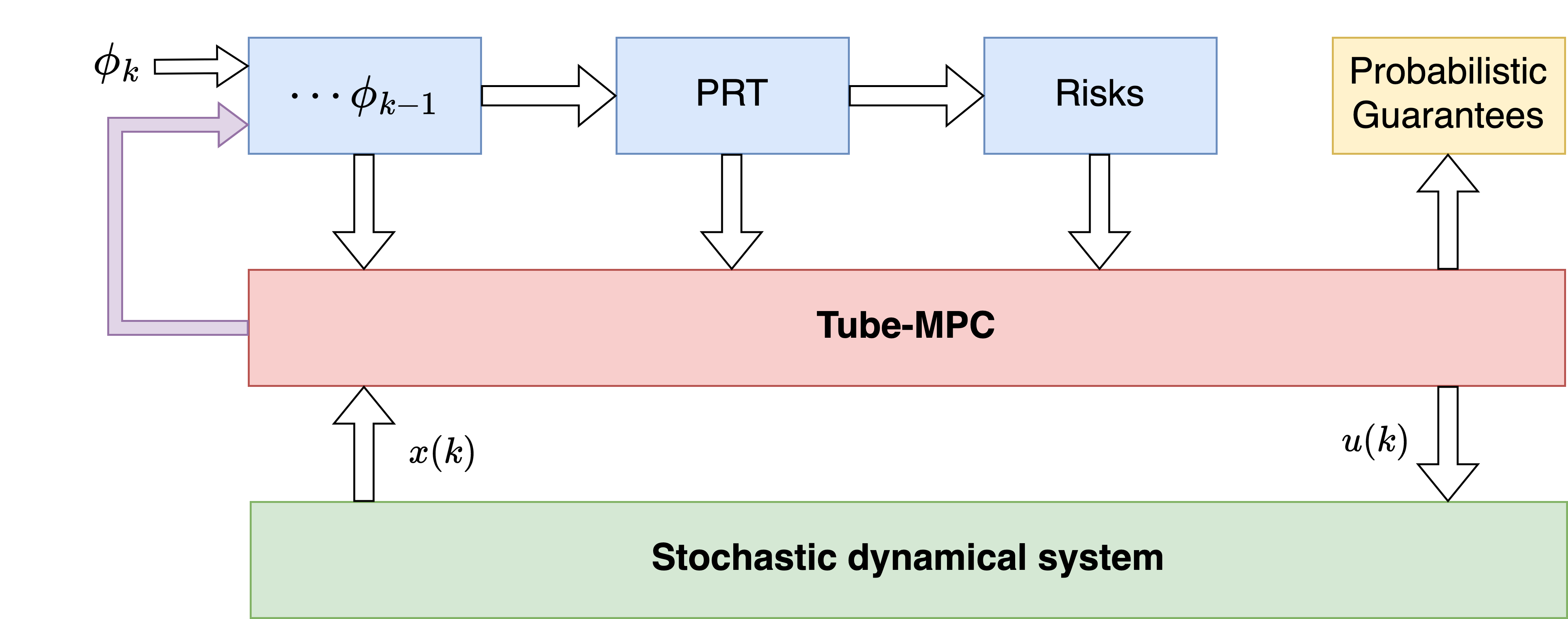
Figure 3: Illustration of the developed approach: real-time specifications, PRTs and risks are dynamically updated and integrated within a deterministic tube-MPC problem, which yields probabilistic guarantees.

3 Risk-Aware Tube-MPC design with Rescheduling

In this section, we will define probabilistic reachable tubes and determine all relevant constraints, c.f. Fig. 3. Next, we introduce a tube-based MPC problem, which will initialize and reschedule the controller per the requirements of both problem statements.

Throughout this section, we decompose the dynamics of (1) into a nominal and an error part. The nominal dynamics, denoted as $z$, contain no stochasticity, and the (stochastic) error dynamics, denoted as $e$, are autonomous. This yields

$$z(k+1) =Az(k)+Bv(k),$$ (4a)

$$e(k+1) =A_{K}e(k)+w(k),$$ (4b)

$$\mbox{with }x(k) =z(k)+e(k),$$ (4c)

$$u(k) =v(k)+Ke(k).$$ (4d)

Here $A_{K}=A+BK$ and $K$ is a stabilizing feedback gain meant to keep the error $e$ small.

3.1 Probabilistic Reachable Tubes

We define probabilistic reachable sets as follows, similar to (Hewing and Zeilinger, 2018).

Definition 2 (Probabilistic Reachable Sets)

A probabilis-tic reachable set (PRS) of dynamic probability level $p$ for error dynamics (4b), denoted by $\mathcal{R}^{p}$, is a set that satisfies

$$e(0)=0\Rightarrow\mathbb{P}(e(k)\in\mathcal{R}^{p})\geq p,\ \forall k\geq 0.$$ (5)

Definition 2 states that a PRS of probability level $p$ will contain at any time instance $k$ the accumulating error $e(k)$ with at least probability $p$, if the initial error satisfies $e(0)=0$. Moreover, due to the invariance property of PRS with respect to the accumulating error, a PRS may be defined at any time and can be moved over the time horizon without this influencing its probability level.

Multiple representations for probabilistic reachable sets exist, including the ellipsoidal representation. For simplicity, we will make the following assumption.

Assumption 1

Distribution $\mathcal{Q}_{w}$ has zero mean.

The above assumption is not necessary to obtain an ellipsoidal representation but will simplify most of the computations. The ellipsoidal representation is obtained from the multivariable Chebyshev inequality; details are given in (Hewing and Zeilinger, 2018). Under Assumption 1, the ellipsoidal representation is given by

$$\mathcal{R}^{p}=\{x\in\mathbb{R}^{n}\mid x^{T}\Sigma_{\infty}^{-1}x\leq\tilde{p}\},$$ (6)

where $\Sigma_{\infty}$ solves the Lyapunov equation

$$A_{K}\Sigma_{\infty}A_{K}^{T}-\Sigma_{\infty}+\text{var}(\mathcal{Q}_{w})=0,$$ (7)

$p$ is the probability level, and

$$\tilde{p}=\frac{n}{1-p}.$$ (8)

Since the variance of $\mathcal{Q}_{w}$ is assumed to be strictly positive definite and $A_{K}$ is stable, Lyapunov theory states that $\Sigma_{\infty}$ is strictly positive definite. Hence, in the sequel, we consider the transformed state and constraints for which $\Sigma_{\infty}=I_{n}$. We call these transformed dynamics the normalized dynamics, and in the remainder, we maintain our notations as if the dynamics are normalized. Notice that each PRS is now a hypersphere with radius $\sqrt{\tilde{p}}$. Accordingly, Eq. (8) is now a relation between the radius and the probability level of each PRS.

Remark 1

In the case of Gaussian disturbance, a less conservative relation exists, compared to Eq. (8). This alternative relation is given by $\tilde{p}=\chi^{2}_{n}(p)$, the inverse cumulative distribution function of the chi-squared distribution with $n$ degrees of freedom.

By defining a PRS $\mathcal{R}^{p_{k}}$ at each time instance $k\in\{0,\cdots,N\}$, we obtain a finite sequence of PRS called a probabilistic reachable tube $\mathcal{R}:=\{\mathcal{R}^{p_{0}},\cdots,\mathcal{R}^{p_{N}}\}$. A probabilistic reachable tube can have either constant or varying diameter, with the former only if $p(i)=p(j)$ for all $i\leq j$. We define the risk level $r_{k}$ as an upper bound on the probability that $\mathcal{R}^{p_{k}}$ does not contain the error $e(k)$.

Lemma 3 (Risk-Aware Tube Lemma)

The risk that errors $\{e(0),\cdots,e(N)\}$ are not contained within a given probabilistic reachable tube $\{\mathcal{R}^{p_{0}},\cdots,\mathcal{R}^{p_{N}}\}$ is at most

$$\bar{r}=\sum_{i=1}^{N}(1-p_{i}).$$ (9)

Proof 3.4.

The probability that the errors are contained within the PRT is given by $p=1-\mathbb{P}(\cup_{i=0}^{N}E_{i})$, where $E_{i}$ is the event that the $i^{\text{th}}$ element of the PRT does not contain the $i^{\text{th}}$ element of the errors. Notice that $\mathbb{P}(E_{0})=0$ and $\mathbb{P}(E_{i})\leq r_{i}=1-p_{i}$. We can lower bound $p$ as follows:

$$\bar{p}=1-\sum_{i=1}^{N}r_{i}\leq 1-\sum_{i=0}^{N}\mathbb{P}(E_{i})\leq 1-\mathbb{P}(\cup_{i=0}^{N}E_{i})=p.$$

The first inequality is due to the probabilistic reachable set relation (5), and the second is due to the union bound argument or Boole’s inequality (Boole, 1847). An upper bound on the risk is then obtained from $\bar{r}=1-\bar{p}$.

3.2 Risk-Aware Tube-MPC Constraints Design

This subsection aims to relate each STL specification $\phi$ assigned at time $k$, by means of a PRT, to the upper bound risk $r_{\phi}^{k}$ of failing an STL specification $\phi$, assigned at time $k$. This way, by constraining $r_{\phi}^{k}\leq r_{\phi,\max}$ at each time step $i\geq k$, we can ensure that all accepted specifications have acceptable probabilistic guarantees.

We first define the active horizon $\mathcal{H}_{\phi}^{k}$ of any specification $\phi$ as the set of all time instances needed to evaluate $\boldsymbol{x}_{k}\vDash\phi$.

Definition 3.5.

The active horizon is recursively given by:

$$\boldsymbol{\vec{x}}_{k}\vDash\top \iff \mathcal{H}_{\top}^{k}=\emptyset$$

$$\boldsymbol{\vec{x}}_{k}\vDash\mu \iff \mathcal{H}_{\mu}^{k}=\{k\}$$

$$\boldsymbol{\vec{x}}_{k}\vDash\lnot\mu \iff \mathcal{H}_{\lnot\mu}^{k}=\{k\}$$

$$\boldsymbol{\vec{x}}_{k}\vDash\phi_{1}\wedge\phi_{2} \iff \mathcal{H}_{\phi_{1}\wedge\phi_{2}}^{k}=\mathcal{H}_{\phi_{1}}^{k}\cup\mathcal{H}_{\phi_{2}}^{k}$$

$$\boldsymbol{\vec{x}}_{k}\vDash\phi_{1}\vee\phi_{2} \iff \mathcal{H}_{\phi_{1}\vee\phi_{2}}^{k}=\mathcal{H}_{\phi_{1}}^{k}\cup\mathcal{H}_{\phi_{2}}^{k}$$

$$\boldsymbol{\vec{x}}_{k}\vDash\square_{[a,b]}\ \phi \iff \mathcal{H}_{\square_{[a,b]}\phi}^{k}=\cup_{i=k+a}^{k+b}\mathcal{H}_{\phi}^{i}$$

$$\boldsymbol{\vec{x}}_{k}\vDash\phi_{1}\ U_{[a,b]}\ \phi_{2} \iff \mathcal{H}_{\phi_{1}\ U_{[a,b]}\ \phi_{2}}=\mathcal{H}_{1}\cup\mathcal{H}_{2}$$

$$\text{ with }\mathcal{H}_{1}=\cup_{i=k}^{k+b}\mathcal{H}_{\phi_{1}}^{i}\text{ and }\mathcal{H}_{2}=\cup_{j=k+a}^{k+b}\mathcal{H}_{\phi_{2}}^{j}.$$

Notice that the suffix $\boldsymbol{x}_{N+1}$ with $N=\max{\mathcal{H}_{\phi}^{k}}$, does not influence the satisfaction of $\boldsymbol{x}_{k}\vDash\phi$. Hence, in the remainder of the paper, we consider only the prefix $\boldsymbol{x}_{[k,N]}:=\{x(k),\cdots,x(N)\}$ and note that $\mathbb{P}_{\boldsymbol{f}}(\phi,k)=\mathbb{P}_{\boldsymbol{f},k}(\vec{\boldsymbol{x}}_{k}\vDash\phi\mid x(k))=\mathbb{P}_{\boldsymbol{f},k}(\vec{\boldsymbol{x}}_{[k,N]}\vDash\phi\mid x(k))$.

Remark 3.6.

The value of $N$ defined above has a close relation to the length $L(\cdot)$ of an STL specification, formally defined in (Maler and Nickovic, 2004). Specifically, for a specification $\phi$ assigned at time $k$ with a length $L(\phi)$, we have $L(\phi)=N-k$.

Given an STL specification $\phi$ assigned at time $k$, Raman et al. (2014) explains that mixed integer linear constraints can represent any STL specification in negation normal form. As can be observed in the following equations, for each time instance $i\in\mathcal{H}_{\phi}^{k}$, these STL specifications define a linear constraint that is parametrized with binary variable $s$, as follows

$$G(i)x(i)+MF(i)s \geq b(M,i)+\rho(i)\boldsymbol{1},$$ (10a)

$$Cs\geq d,\ \epsilon\leq\rho(i) \leq\frac{M}{2},\ \forall i\in\mathcal{H}_{\phi}^{k},$$ (10b)

where $G(i)$, $E(i)$, $C$ and $b(M,i)$, $d$ are, respectively, matrices and vectors of appropriate sizes; $M$ is a large positive number; $\epsilon$ is a small positive number; and $\rho(i)>0\in\mathbb{R}$ is a positive real number. For more information on the derivation, consider the Appendix.

From robustness per time instance $i$ to risk. Note that $\rho(i)$ performs a similar function as the robustness notion in (Donzé and Maler, 2010). However, unlike those notions, we have opted for a local notion of robustness for the $i$-th time instance. That is, $\rho(i)$ defines the slack available in the constraints active for the state $x(i)$. Furthermore, given that the predicates are normalized, $\rho(i)$ denotes the minimal distance between the state $x(i)$ and the active constraints. This crucially determines the maximal radii of the probabilistic reachable tube for which the constraints are still satisfied. Thereby, we can quantify the risk $r_{\phi}^{k}$ as given in the following theorem.

Theorem 3.7.

Let specification $\phi$ be assigned at time $k$ to the system (4) with normalized dynamics. If the nominal trajectory $\{z(k),\cdots,z(N)\}$ with $z(k)=x(k)$ and nominal controls $\{v(k),\cdots,v(N-1)\}$ satisfies (10) with $\{\rho(k),\cdots,\rho(N)\}$ strictly positive, than

$$\mathbb{P}_{\boldsymbol{f}}(\phi,k)=\mathbb{P}_{\boldsymbol{f},k}(\vec{\boldsymbol{x}}_{k}\vDash\phi\mid x(k))\geq 1-r_{\phi}^{k},$$

where risk $r_{\phi}^{k}$ is at most

$$r_{\phi}^{k}=\sum_{i\in\mathcal{H}_{\phi}^{k}\backslash\{k\}}\frac{n}{\rho(i)^{2}}.$$ (11)

Proof 3.8.

The nominal trajectory $\mathbf{z}_{[k,N]}$ satisfies the specification $\phi$ since $\rho(i)$ is positive for all $i$. We now need to prove the lower bound of the satisfaction probability based on the actual trajectory $\boldsymbol{x}_{[k,N]}$ that is affected by the noise. Given the sequence of $\rho$ values we know that $\boldsymbol{x}_{[k,N]}$ satis-fies the specification if $\forall i\in\mathcal{H}_{\phi}^{k}\backslash\{k\}$ the error $e(i)$ is con-strained as $\|e(i)\|\leq\rho(i)$. Based on Lemma 3 and Eq. (8), we have than that $\mathbb{P}_{\boldsymbol{f}}(\phi,k)\geq 1-r_{\phi}^{k}$ with $r_{\phi}^{k}$ as in (11).

3.3 Risk-Aware Tube-MPC Rescheduling

Utilizing the relation between STL specifications and their risks, established during the previous subsection, we first consider the general case in which we constrain the risks to maintain the probabilistic guarantees on the satisfaction of previously accepted specifications. Afterwards, we consider the special case in which new specifications are provided in real-time. Both cases will result in tube-based MPC problems, which we solve recursively at each time instance.

Preserving risks bounds with Tube-MPC. We consider multiple specifications at the same time. For each of these specifications $\pi$, we denote with $k_{\pi}$ the time at which the specification was accepted. We denote with $\mathcal{P}^{k}$ the set of all accepted specifications $\pi$ at time $k$ with $k_{\pi}\leq k$. Therefore, at time $k$ we are controlling the system to satisfy $\phi=\wedge_{\pi\in\mathcal{P}^{k}}\lozenge_{[k_{\pi},k_{\pi}]}\pi$. Each part of this specification $\pi$ has an individual maximal risk $r_{\pi,\max}$.

We are now interested in implementing an MPC algorithm that at each time instance $k\in[0,N]$ recomputes the optimal nominal trajectory $\boldsymbol{z}_{[k,N]}$, the optimal nominal input $\boldsymbol{v}_{[k,N-1]}$, and the optimal risk levels $\boldsymbol{r}_{[k,N]}$. For this, we assume given $x(k)$ together with $\boldsymbol{z}_{[0,k]}$, $\boldsymbol{v}_{[0,k-1]}$ and $\boldsymbol{r}_{[0,k]}$ computed at time $k-1$. Furthermore, for all $\pi\in\mathcal{P}^{k}$, we assume $\mathcal{H}_{\pi}^{k_{\pi}}\subseteq[0,N]$.

Let us consider the following tube-based MPC problem

$$\min_{\Xi}\ J(\boldsymbol{z}_{[0,N]},\boldsymbol{v}_{[0,N-1]},\boldsymbol{r}_{[0,N]})+Ma(k),$$ (12a)

s.t. $$z(k)=(1-a(k))x(k)+a(k)z_{k},\ a(k)\in\{0,1\},\!\!$$ (12b)

$$z(i+1)=Az(i)+Bv(i),\forall i\in\{k,\cdots,N-1\},\!\!$$ (12c)

$$G(j)z(j)+MF(j)s(k)\geq b(M,j)+\rho(j)\boldsymbol{1},$$ (12d)

$$Cs(k)\geq d,\ \epsilon\leq\rho(j)\leq\textstyle\frac{M}{2},\ \forall j\in\{0,\cdots,N\},$$ (12e)

$$n=\rho(j)^{2}r(j),\hskip 56.9055pt\forall j\in\{0,\cdots,N\},$$ (12f)

$$\textstyle\sum_{\{j\in\mathcal{H}_{\pi}^{k_{\pi}}\setminus k_{\pi}\}}\ r(j)\leq r_{\pi,\max},\hskip 28.45274pt\forall\pi\in\mathcal{P}^{k},$$ (12g)

where $\Xi:=\{\boldsymbol{z}_{[k,N]},\boldsymbol{v}_{[k,N-1]},\boldsymbol{r}_{[k+1,N]},s(k),a(k)\}$, $z_{k}$ is the last element of $\boldsymbol{z}_{[0,k]}$, $J$ is either a linear or quadratic cost function, and the constraints (12d)-(12e) are obtained from $\phi=\wedge_{\pi\in\mathcal{P}^{k}}\lozenge_{[k_{\pi},k_{\pi}]}\pi$.

At $k=0$, the MPC problem, initialized with $z_{0}=x(0)$, will find a controller $\boldsymbol{f}$ composed of the optimal nominal trajectory $\boldsymbol{z}_{[0,N]}$, the optimal nominal input $\boldsymbol{v}_{[0,N-1]}$, and the optimal risk levels $\boldsymbol{r}_{[0,N]}$. Note that in this case, Eq. (12b) is trivially satisfied for $z(0)=z_{0}=x(0)$. Therefore, in this case, Theorem 3.7 will hold and for each of the specifications $\pi\in\mathcal{P}^{0}$ the maximal risk $r_{\pi,\max}$ is satisfied if the computed nominal input sequence $\boldsymbol{v}_{[0,N-1]}$ is applied.

At $k>0$, we remark that constraint (12b) considers either the previously computed nominal state $z(k)$ or the measured state $x(k)$, similar to (Hewing and Zeilinger, 2018). In the former case, the previously computed nominal input will be applied and this will also preserve the previously computed risk levels. In the latter case, with $z(k)=x(k)$ the MPC algorithm will yield a recomputed optimal nominal trajectory $\boldsymbol{z}_{[k,N]}$, optimal nominal input $\boldsymbol{v}_{[k,N-1]}$, and optimal risk levels $\boldsymbol{r}_{[k+1,N]}$. Due to Definition 2, we can use (Hewing and Zeilinger, 2018; Engelaar et al., 2023) to show that this guarantees $\mathbb{P}_{\boldsymbol{f}}(\pi,k_{\pi})\geq 1-\sum_{\{j\in\mathcal{H}_{\pi}^{k_{\pi}}\setminus k_{\pi}\}}\ r(j)$ for each $\pi\in\mathcal{P}^{k}$. This, together with constraint (12g), ensures risk bounds on previously accepted specifications are maintained.

To ensure a linear or quadratic programming scheme is viable in solving optimization problem (12), the non-linear expression can be replaced by a piece-wise linear function that over-approximates the risk levels $r(j)$. By over-approximating the risk levels, $r_{\pi}^{k_{\pi}}$ will become more conservative and thus remain valid. To mitigate this conservativeness, we can increase the number of piece-wise elements within the linear over-approximation.

Up to now, we have implicitly assumed that $\mathcal{P}^{k-1}=\mathcal{P}^{k}$. In case specifications arrive in real-time, this will not hold.

Real-time Specifications. Let $\psi$ be a newly assigned specification, $\mathcal{P}^{k}=\mathcal{P}^{k-1}\cup\psi$. To maintain probabilistic guarantees on the satisfaction of all previously accepted specifications and be able to either accept or reject the new specification, we consider the following tube-based MPC problem, given by

$$P_{k}:\min_{\Xi,c(k)}\ J(\boldsymbol{z}_{[0,N]},\boldsymbol{v}_{[0,N-1]},\boldsymbol{r}_{[0,N]})+Ma(k)+Mc(k),\!\!$$ (13a)

s.t. $$z(k)=(1-a(k))x(k)+a(k)z_{k},\ a(k)\in\{0,1\},\!\!$$

$$z(i+1)=Az(i)+Bv(i),\ i\in\{k,\cdots,N-1\},\!\!$$

$$\text{constraints }\eqref{Eq:TMPC_SpecOld}-\eqref{Eq:TMPC_ProbGuar}\text{ for }\pi\in\mathcal{P}^{k-1},$$

$$\bar{G}(j)z(j)+M\bar{F}(j)s(k)\geq\bar{b}(M,j)$$ (13b)

$$\hskip 113.81102pt+(\rho(j)-c(k)M^{2})\boldsymbol{1},$$

$$c(k)\geq a(k),\ c(k)\in\{0,1\},$$ (13c)

$$\textstyle\sum_{\{j\in\mathcal{H}_{\psi}^{k}\setminus k\}}r(j)\leq r_{\psi,\max}+c(k)M,\!\!\!$$ (13d)

where again the constraint (13b) is obtained from $\psi$. We remark that constraint (13c) ensures that a new specification will be accepted only if $z(k)=x(k)$, while inequality (13d) ensures a bound on the risk only if the specification is accepted ($c(k)=0$).

Combining the steps in the previous section to compute the probabilistic reachable sets, normalize the dynamics, and writing out the specifications with the above MPC problem, we get the following algorithm to reschedule the controller during runtime and synthesize a control input.

Algorithm 1 Control rescheduling algorithm

1:Given: System (1) initialized at $x(0)$

2:Determine $K$ and compute $\Sigma_{\infty}$ from Eq. (7)

3:Get normalized dynamics of (1)

4:Set $k=0$, $z_{0}=x(0)$

5:for $k\in\{0,N-1\}$ do

6:     if no new specification then go to line 14

7:     Rescheduling MPC with old and new specifications:

8:     ($\psi$, $r_{\psi,\max}$) $\leftarrow$ load new specification

9:     Solve (13) to get $\boldsymbol{z}_{[k,N]}$, $\boldsymbol{v}_{[k,N-1]}$, $\boldsymbol{r}_{[k+1,N]}$, $c(k)$

10:     if $c(k)=1$ then go to line 14 $\triangleright$ $\psi$ is infeasible

11:     Set $\mathcal{P}^{k}=\mathcal{P}^{k-1}\cup\psi$ $\triangleright$ $\psi$ is added

12:     go to line 16

13:     MPC with only old specifications:

14:     Solve (12) to get $\boldsymbol{z}_{[k,N]}$, $\boldsymbol{v}_{[k,N-1]}$, $\boldsymbol{r}_{[k+1,N]}$

15:     Implement control

16:     Compute $u(k)$ from Eq. (4)

17:     Implement $u(k)$, and measure $x(k+1)$

18:end for

Theoretical Analysis. As shown next, the tube-MPC problem (13) is recursively feasible.

Theorem 3.9.

For all $k\in\{1,\cdots,N\}$, and all $x(k)\in\mathbb{R}^{n}$, if the tube-MPC problem $P_{k-1}$ defined in (13) is feasible, then the corresponding problem $P_{k}$ at the next time instant remains feasible.

Proof 3.10.

Let $\boldsymbol{z}_{[0,N]}$, $\boldsymbol{v}_{[0,N-1]}$ and $\boldsymbol{r}_{[0,N]}$ be solutions of $P_{k-1}$. Take $a(k)=c(k)=1$ and notice that constraints (12b)-(12c) are satisfied by $\boldsymbol{z}_{[0,N]}$, $\boldsymbol{v}_{[0,N-1]}$ and $a(k)=1$ for $P_{k}$. Notice that constraints (12d)-(12g), and (13b)-(13d) in $P_{k-1}$ are equivalent to constraints (12d)-(12g) in $P_{k}$. Hence, $\boldsymbol{z}_{[0,N]}$, $\boldsymbol{v}_{[0,N-1]}$ and $\boldsymbol{r}_{[0,N]}$ satisfy constraints (12d)-(12g) for $P_{k}$. Finally, by taking $c(k)=1$ constraints (13b)-(13d) are also trivially satisfied. We conclude that $\Xi=\{\boldsymbol{z}_{[0,N]},\boldsymbol{v}_{[0,N-1]},\boldsymbol{r}_{[0,N]},a(k),c(k)\}$ is a solution to $P_{k}$. Hence, if $P_{k-1}$ is feasible, then $P_{k}$ is feasible.

For each of the specifications $\pi\in\mathcal{P}^{N}$ accepted by $k=N$ in Algorithm 1, we need to have that

$$\mathbb{P}_{\boldsymbol{f}}(\pi,k_{\pi})\geq 1-r_{\pi,\max}.$$ (14)

To show that this holds, it is sufficient to show that if at $k=0$, the optimal solution with $\boldsymbol{r}^{(k=0)}_{[0,N]}$ is such that

$$\textstyle\sum_{\{j\in\mathcal{H}_{\pi}^{k_{\pi}}\setminus k_{\pi}\}}\ r^{(k=0)}(j)\leq r_{\pi,\max},$$

then the open-loop implementation will satisfy (14). This would equate to solving (12) and(13) with $z(k)=z_{k}$. Additionally, as shown in (Hewing and Zeilinger, 2018, Theorem 3), if we instead use the updated state $z(k)=x(k)$, we still strictly preserve the original probability bounds due to the definition of the probabilistic reachable sets and the unimodal convexity of the additive disturbance.

4 Numerical Simulation

Consider a two-dimensional robot-motion planning case to validate the efficacy of the proposed control rescheduling method. The dynamic model of the robot is described by Eq. (1) with $A=B=I_{2}$, $x(0)=(0,0)$, $n=2$, and $w(k)\sim\mathcal{N}(0,\sigma I_{2})$ independent for all $k\in\{0,\cdots,N-1\}$, with $\sigma=0.002$. We consider a finite time-horizon $N=40$, a stabilizing feedback gain $K\approx 0.618I_{2}$ for Eq. (4b), a maximal risk $r_{\pi,\max}=0.5$ for any specification $\pi$ and a cost $J(\boldsymbol{z},\boldsymbol{v})=u^{T}Ru+\sum_{i=1}^{N}r(i)$ for Eq. (13a) with $R=0.001I_{2}$. A coordinate transformation is performed to ensure all PRS are spherical and the dynamics are normalized.

Instead of the non-linear constraints (12f), we impose the following equality and inequality constraints, which imply that the original constraints hold. These constraints are computationally preferable, as they are quadratic convex equality and linear inequality constraints, respectively. We replace the non-linear equality (12f) with a quadratic equality $r(k)=a\rho(k)^{2}+b$ and a linear inequality $0.01\leq r(k)\leq 1$, with $a=-0.005$ and $b=1.01$. It is easy to verify that $a\rho(k)^{2}+b\geq\frac{n}{\rho(k)^{2}}$ always holds for $r(k)\in[\,0.01,1\,]$. Therefore, the transformed optimization problem provides a sound solution to obtaining valid upper bound risks $r_{\phi}^{k}$.

The motion planning scenario is illustrated in Fig. 4 which contains a safety set $S:=\{(x_{1},x_{2})\in\mathbb{R}^{2}\mid-10\leq x_{1}\leq 10\text{ and }-2\leq x_{2}\leq 10\}$, a home set $H:=\{(x_{1},x_{2})\in\mathbb{R}^{2}\mid-10\leq x_{1}\leq 10\text{ and }-2\leq x_{2}\leq 0\}$, an obstacle $O:=\{(x_{1},x_{2})\in\mathbb{R}^{2}\mid-2\leq x_{1}\leq 2\text{ and }3\leq x_{2}\leq 10\}$, two targets $T_{1}:=\{(x_{1},x_{2})\in\mathbb{R}^{2}\mid-10\leq x_{1}\leq-8\text{ and }8\leq x_{2}\leq 10\}$ and $T_{2}:=\{(x_{1},x_{2})\in\mathbb{R}^{2}\mid 7\leq x_{1}\leq 9\text{ and }7\leq x_{2}\leq 9\}$, and a charger $C:=\{(x_{1},x_{2})\in\mathbb{R}^{2}\mid-8\leq x_{1}\leq-3\text{ and }2\leq x_{2}\leq 4\}$. Note that all sets above are rectangular and can easily be represented as normalized polyhedral predicates.

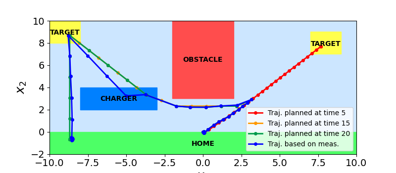
Figure 4: The red, orange and green trajectory show robotic movement planned at $k=5$, $k=15$ and $k=20$ respectively. The blue trajectory shows the robots’ actual movement.

This case study considers a reach-avoid problem in which new reach objectives are dynamically assigned. More precisely, the specifications $\{\phi_{0},\phi_{1},\phi_{2},\phi_{3}\}$ are assigned to the robot at times $k=0,\ k=5,\ k=15$ and $k=20$, respectively. Here $\phi_{0}:=\square_{[0,40]}\left[(x(k)\in S)\wedge\lnot(x(k)\in O)\right]$, $\phi_{1}:=\lozenge_{[20,30]}\left[(x(k)\in T_{1})\vee(x(k)\in T_{2})\right]$, $\phi_{2}:=\lozenge_{[20,25]}(x(k)\in C)$, and $\phi_{3}:=\lozenge_{[25,30]}\square_{[0,5]}(x(k)\in H)$. Additionally, we specify that the control inputs are limited by $-2\leq u(k)\leq 2$ for all $k\in\{0,1,\cdots,N-1\}$. We use the stlpy toolbox to synthesize our controller (Kurtz and Lin, 2022). The results are shown in Fig. 4 and Table 1.

	$\phi_{0}$	$\phi_{1}$	$\phi_{2}$	$\phi_{3}$
$k=k_{i}$	0.40	0.10	0.05	0.10
$k=N$	0.40	0.10	0.05	0.10

Table 1: A table containing the upper bound risks of $\phi_{i}$ at time of acceptance $k_{i}$ and after runtime.

From Fig. 4, we notice that at time $k=5$, the robot was scheduled to move towards the right target, only for it to move to the left target when it was additionally tasked with recharging its battery at time $k=15$. This result clearly illustrates that our control scheme allows the robot to make changes during runtime to accomplish as many tasks as possible. Additionally, upper bound risks on specifications, see Table 1, remained below the maximum of $r_{\pi,\max}=0.5$. This result illustrates the ability to obtain valid probabilistic guarantees. Finally, it can be seen that state updates likely influence the robot’s movement since the blue trajectory clearly differs from the green trajectory around the charger, something which is unlikely to be attributed only to the additive disturbances due to the variance being relatively small.

5 Conclusion

In this paper, we developed a formal rescheduling control scheme for linear stochastic systems that must satisfy dynamically assigned specifications while preserving the performance of existing specifications. This was achieved by integrating real-time specification updates with probabilistic reachable tubes, risks and tube-MPC algorithms. A limitation of the developed approach is the conservativeness introduced in the upper bound risks due to the probabilistic reachable tubes and the union-bound argument. Relaxing this further will be considered in future work. We will also investigate an extension of the method to multi-agent systems, where specifications rejected by one agent are assigned to other agents within the system.

Appendix

Additional information on minimal distances.

The minimal distance between a point $\bar{x}$ and a normalized hyperplane $g^{T}x=b$, i.e., $||g||=1$, is given by $l=|g^{T}\bar{x}-b|$.

Additional information on the derivations of (10).

In (Raman et al., 2014, IV-B), each predicate $\mu$ can be represented by two inequality constraints and a binary variable $s_{k}^{\mu}$. Here, the constraints enforce that $s_{k}^{\mu}=1$ if the predicate is satisfied at time step $k$, i.e. $h(\boldsymbol{x}(k))\geq 0$. Utilizing the notation of this paper with minor simplification, these inequality constraints are given by

$$h(\boldsymbol{x}(k)) \geq(M(s_{k}^{\mu}-1)+\epsilon)\boldsymbol{1}_{q},$$ (15a)

$$-h(\boldsymbol{x}(k)) \geq(\epsilon-Ms^{\mu}_{k})\boldsymbol{1}_{q},$$ (15b)

where $M$ is a large positive number and $\epsilon$ is a small positive number. Notice that, should the predicate be satisfied at time $k$, $h(\boldsymbol{x}(k))\geq\epsilon\boldsymbol{1}_{q}$. By replacing $\epsilon$ with $\rho(k)$, we can also consider the minimal distance between the state $\boldsymbol{x}(k)$ and the hyperplane boundaries of the normalized polyhedron predicate. To ensure the constraints remain valid, we assume that $\epsilon\leq\rho(k)\leq\frac{M}{2}$, ensuring that $\rho(k)-M$ is a large negative number, similar to $\epsilon-M$.

References

- Bertsekas and Shreve (1996) Bertsekas, D. and Shreve, S.E. (1996). Stochastic optimal control: the discrete-time case, volume 5. Athena Scientific.
- Boole (1847) Boole, G. (1847). The mathematical analysis of logic. Philosophical Library.
- Bruno and Antonelli (2018) Bruno, G. and Antonelli, D. (2018). Dynamic task classification and assignment for the management of human-robot collaborative teams in workcells. The International Journal of Advanced Manufacturing Technology, 98, 2415–2427.
- Dharmadhikari and Jogdeo (1976) Dharmadhikari, S. and Jogdeo, K. (1976). Multivariate unimodality. The Annals of Statistics, 607–613.
- Donzé and Maler (2010) Donzé, A. and Maler, O. (2010). Robust satisfaction of temporal logic over real-valued signals. In International Conference on Formal Modeling and Analysis of Timed Systems, 92–106. Springer.
- Engelaar et al. (2023) Engelaar, M., Haesaert, S., and Lazar, M. (2023). Stochastic model predictive control with dynamic chance constraints. In 27th International Conference on System Theory, Control and Computing, 356–361.
- Farahani et al. (2018) Farahani, S.S., Majumdar, R., Prabhu, V.S., and Soudjani, S. (2018). Shrinking horizon model predictive control with signal temporal logic constraints under stochastic disturbances. IEEE Transactions on Automatic Control, 64(8), 3324–3331.
- Farahani et al. (2017) Farahani, S.S., Majumdar, R., Prabhu, V.S., and Soudjani, S.E.Z. (2017). Shrinking horizon model predictive control with chance-constrained signal temporal logic specifications. In 2017 American Control Conference (ACC), 1740–1746. IEEE.
- Farahani et al. (2015) Farahani, S.S., Raman, V., and Murray, R.M. (2015). Robust model predictive control for signal temporal logic synthesis. IFAC-PapersOnLine, 48(27), 323–328.
- Hewing and Zeilinger (2018) Hewing, L. and Zeilinger, M.N. (2018). Stochastic model predictive control for linear systems using probabilistic reachable sets. In 2018 IEEE Conference on Decision and Control (CDC), 5182–5188.
- Kurtz and Lin (2022) Kurtz, V. and Lin, H. (2022). Mixed-integer programming for signal temporal logic with fewer binary variables. IEEE Control Systems Letters, 6, 2635–2640.
- Maler and Nickovic (2004) Maler, O. and Nickovic, D. (2004). Monitoring temporal properties of continuous signals. In International Symposium on Formal Techniques in Real-Time and Fault-Tolerant Systems, 152–166. Springer.
- Mehr et al. (2017) Mehr, N., Sadigh, D., Horowitz, R., Sastry, S.S., and Seshia, S.A. (2017). Stochastic predictive freeway ramp metering from signal temporal logic specifications. In 2017 American Control Conference, 4884–4889. IEEE.
- Mustafa et al. (2023) Mustafa, K.A., de Groot, O., Wang, X., Kober, J., and Alonso-Mora, J. (2023). Probabilistic risk assessment for chance-constrained collision avoidance in uncertain dynamic environments. arXiv preprint arXiv:2302.10846.
- Raman et al. (2014) Raman, V., Donzé, A., Maasoumy, M., Murray, R.M., Sangiovanni-Vincentelli, A., and Seshia, S.A. (2014). Model predictive control with signal temporal logic specifications. In 53rd IEEE Conference on Decision and Control, 81–87. IEEE.
- Raman et al. (2015) Raman, V., Donzé, A., Sadigh, D., Murray, R.M., and Seshia, S.A. (2015). Reactive synthesis from signal temporal logic specifications. In Proceedings of the 18th international conference on hybrid systems: Computation and control, 239–248.
- Sadigh and Kapoor (2015) Sadigh, D. and Kapoor, A. (2015). Safe control under uncertainty. arXiv preprint arXiv:1510.07313.
- Sadigh and Kapoor (2016) Sadigh, D. and Kapoor, A. (2016). Safe control under uncertainty with probabilistic signal temporal logic. In Proceedings of Robotics: Science and Systems XII.
- Sadraddini and Belta (2015) Sadraddini, S. and Belta, C. (2015). Robust temporal logic model predictive control. In 2015 53rd Annual Allerton Conference on Communication, Control, and Computing (Allerton), 772–779. IEEE.
- Sadraddini and Belta (2019) Sadraddini, S. and Belta, C. (2019). Formal synthesis of control strategies for positive monotone systems. IEEE Transactions on Automatic Control, 64(2), 480–495.
- Zhu and Yang (2006) Zhu, A. and Yang, S.X. (2006). A neural network approach to dynamic task assignment of multirobots. IEEE transactions on neural networks, 17(5), 1278–1287.