Optimal and Near-Optimal Adaptive Vector Quantization

Abstract

Quantization is a fundamental optimization for many machine-learning use cases, including compressing gradients, model weights and activations, and datasets. The most accurate form of quantization is adaptive, where the error is minimized with respect to a given input, rather than optimizing for the worst case. However, optimal adaptive quantization methods are considered infeasible in terms of both their runtime and memory requirements.

We revisit the Adaptive Vector Quantization (AVQ) problem and present algorithms that find optimal solutions with asymptotically improved time and space complexity. We also present an even faster near-optimal algorithm for large inputs. Our experiments show our algorithms may open the door to using AVQ more extensively in a variety of machine learning applications.

1 Introduction

Quantization is a central building block for optimizing a large range of machine learning applications. It is often used for compressing gradients to reduce network requirements in distributed and federated learning (e.g., Suresh et al. (2017); Konečnỳ & Richtárik (2018); Caldas et al. (2018); Vargaftik et al. (2022); Dorfman et al. (2023)); for reducing memory footprint while accelerating the computation via post-training quantization (e.g., Frantar et al. (2023); Jeon et al. (2023)), quantization-aware training of models (e.g., Micikevicius et al. (2018); Shen et al. (2020)) and LLMs key-value (KV) cache (Sheng et al., 2023); and for quantization of datasets for faster training and inference (e.g., Zhou et al. (2023)).

A fundamental quantization method is stochastic quantization, where a sender quantizes an input vector $X\in\mathbb{R}^{d}$ using a set $Q\subset\mathbb{R}$ of $|Q|=s$ quantization values in an unbiased manner (Ben Basat, Ran and Mitzenmacher, Michael and Vargaftik, Shay, 2021). That is, each coordinate $x\in X$ is quantized into a value $\widehat{x}\in Q$ such that $\mathbb{E}\left[\widehat{x}\right]=x$. The Adaptive Vector Quantization (AVQ) problem (e.g., Zhang et al. (2017); Fu et al. (2020); Faghri et al. (2020)) then lies in selecting the set $Q$ to minimize the mean squared error given by

$$\mathbb{E}\left[\left\lVert\widehat{X}-X\right\rVert_{2}^{2}\right]=\sum_{x\in X}\mathrm{Var}{[}\widehat{x}]\,\,,$$

also known as the sum of variances.

Previous quantization works can largely be categorized into two classes. The first includes methods that are distribution-agnostic, i.e., design the quantization without optimizing it for the specific input. For example, Stochastic Uniform Quantization (Suresh et al., 2017), QGSD (Alistarh et al., 2017), and Natural Compression (Horvóth et al., 2022) determine the quantization values with respect to global properties such as the vector’s norm, or min and max values.

Other works, including Suresh et al. (2017); Caldas et al. (2018); Safaryan et al. (2020); Vargaftik et al. (2021, 2022); Basat et al. (2022), apply a reversible transformation that converts $X$ into a vector $X^{\prime}$ with controlled distribution (e.g., with $\max(X^{\prime})-\min(X^{\prime})=\tilde{O}(\left\lVert X\right\rVert/\sqrt{d})$), thus allowing quantizing $X^{\prime}$ in a way that optimizes the worse-case sum of variances. The receiver then applies the inverse transform on the quantization of $X^{\prime}$ to obtain an estimate of $X$.

The second class, which addresses the AVQ problem, uses the fact that in many cases the quantized inputs have a significant structure that can be leveraged to reduce the error. For example, DNN gradients (which are often compressed in distributed and federated learning applications to reduce bandwidth (Konečný et al., 2017; Li et al., 2024)) were observed to follow log-normal-like (Chmiel et al., 2021) or normal-like (Banner et al., 2019; Ye et al., 2020) distributions, while sub-Weibull characterizes the distribution of deep activation layers (Vladimirova et al., 2018).

Adaptive methods therefore ask: how can we optimize the choice of $Q$ for a given input $X$?

The answer to this question proves tricky, with the problem being non-convex even for $s{=}4$ (two-bit quantization) (Faghri et al., 2020). Thus, solutions like ZipML (Zhang et al., 2017) approach the challenge using a dynamic programming approach that allows one to optimize $Q$ in polynomial time. However, this solution has a significant overhead and solving the problem optimally is often considered to be infeasible; for example, (Faghri et al., 2020) develop approximate solutions as they write,

“To find the optimal sequence of quantization values, a dynamic program is solved whose computational and memory cost is quadratic in the number of points … For this reason, ZipML is impractical for quantizing on the fly”.

As another evidence of the problem’s hardness, Fu et al. (2020) solve the problem only for a given (Weibull) distribution, writing that

“The empirical distribution is usually non-differentiable, making the searching of $Q$ infeasible”.

Nevertheless, there is a significant interest in advancing AVQ solutions towards wider adoption as even approximate adaptive solutions like ALQ (Faghri et al., 2020) were shown to be more precise than advanced distribution-agnostic methods such such Non-Uniform QSGD (NUQSGD) (Ramezani-Kebrya et al., 2021). Moreover, AVQ methods can improve more complex schemes (e.g., including the aforementioned ones that utilize worst-case to average-case transformations) by replacing distribution-agnostic quantization with an adaptive one.

In this paper, we show that one can, in fact, solve the problem optimally and efficiently. To this end, we introduce QUantized Adaptive Vector EncodeR (QUIVER), an algorithm that features novel acceleration methods and leverages concaveness properties of the underlying problem to reduce the runtime complexity from $O(s\cdot d^{2})$ to $O(s\cdot d)$ and the space complexity from $O(d^{2})$ to $O(s\cdot d)$. We then further accelerate QUIVER by deriving a closed from solution for $s=3$, allowing it to place two quantization values at a time. Finally, we show that one can achieve a $1+o(1)$ approximation in $O(d)+\widetilde{O}(s\cdot\sqrt{d})$ time and space complexities, allowing QUIVER to quantize large vectors on the fly.

We implement our algorithms in C++ and show that QUIVER can, e.g., compute the optimal quantization values for a vector with $1M$ entries in $250ms$ and compute a $1.005$-approximation for a $133M$-sized vector in under a millisecond on a commodity PC. We evaluate our solutions compared to the state of the art AVQ methods on a variety of distributions that are of interest, vector sizes, number of quantization values, and approximation ratios, and demonstrate a speed up of (up to four) orders of magnitude.

We note that there are many works that investigate different forms of compression, including non adaptive quantization, sparsification, low-rank decomposition, variable-length coding and more. Many of these are orthogonal to our work and can be used in conjunction with it. For example, one can use AVQ to quantize a sparsified vector or apply variable length encoding to further reduce the quantization size.

2 Preliminaries

2.1 Notations and definitions

Given two quantization values $a,b$ and a number $x\in[a,b]$, Stochastic Quantization (SQ) is a procedure that rounds $x$ to $\widehat{x}$ where $\widehat{x}\in\left\{a,b\right\}$. Specifically, $\widehat{x}$ obtains the value $a$ with probability $p_{a}=\frac{b-x}{b-a}$ and the value $b$ with probability $p_{b}=\frac{x-a}{b-a}$ (i.e., $p_{a}+p_{b}=1$). An important property of SQ is that the expected rounded value is unbiased, i.e.,

$$\mathbb{E}\left[\widehat{x}\right]=a\cdot p_{a}+b\cdot p_{b}=x.$$

The variance of stochastically quantizing $x$ is then given by

$$\mathbb{E}\left[(x-\widehat{x})^{2}\right]=(x-a)^{2}\cdot p_{a}+(x-b)^{2}\cdot p_{b}=(b-x)(x-a).$$

Given a vector $X\in\mathbb{R}^{d}$ and an integer $s\in\mathbb{N}$, the Adaptive Vector Quantization (AVQ) problem (Zhang et al., 2017; Faghri et al., 2020; Fu et al., 2020) looks for a set of quantization values $Q$ where $|Q|=s$ and that minimizes the mean squared error (MSE) resulting in stochastically quantizing $X$ to $\widehat{X}\in Q^{d}$. That is, each entry $x\in X$ is stochastically quantized between $a_{x}=\max\left\{q\in Q\mid q\leq x\right\}$ and $b_{x}=\min\left\{q\in Q\mid q\geq x\right\}$.

Formally, AVQ seeks to minimize the MSE, given by

$$\mathbb{E}\left[\left\lVert X-\widehat{X}\right\rVert^{2}\right]=\sum_{x\in X}(b_{x}-x)(x-a_{x}),$$

where $\mathbb{E}\left[\widehat{X}\right]=X$ holds by construction.

2.2 Existing AVQ methods

Leveraging the properties that any optimal solution must include $\min X$ and $\max X$ and that there exists an optimal solution in which $Q\subseteq X$ (Zhang et al., 2017), one can naively solve the problem in $O\left({d-2\choose s-2}\right)=d^{\Theta(s)}$ time by going over all choices for the quantization values (as mentioned, the AVQ problem is non-convex for any $s>3$). Instead, we present the following dynamic program (DP) that allows us to solve it optimally and efficiently for any $s$. Given a sorted vector $X=\left\langle x_{1},\ldots,x_{d}\right\rangle$, we denote by $\mathit{MSE}[i,j]$ the optimal MSE of quantizing the prefix vector $X_{j}=\left\langle x_{1},\ldots,x_{j}\right\rangle$ using $i$ quantization values that include $x_{j}$. Our goal is then to compute $\mathit{MSE}[s,d]$ and a quantization values set $Q$ that obtains it. Accordingly, we express the dynamic program as follows. To begin, we define $C[k,j]$ as the sum of variances of all entries in the range $[x_{k},x_{j}]$, i.e.,

$$C[k,j]=\sum_{x\in[x_{k},x_{j}]}(x_{j}-x)(x-x_{k})\ \ .$$

Here and when clear from context, to simplify notation, we write $\sum_{x}$ to denote $\sum_{x\in X}$.

For $i\in[2,s],j\in[i,d]$, we set $\mathit{MSE}[2,j]=C[1,j]\,\,\forall j$ and use the recurrence

$$\mathit{MSE}[i,j]=\min\limits_{k\in\left\{i,\ldots,j\right\}}\ \mathit{MSE}[i-1,k]+C[k,j]~{}.$$

Here, the index $k$ denotes the coordinate in $X$, $x_{k}$, of the rightmost quantization value to the left of $x_{j}$. A naive solution for the above DP is first to compute the matrix $C$ (which takes $O(d^{3})$ time and $O(d^{2})$ space) and then calculate $\mathit{MSE}[s,d]$ in $O(s\cdot d^{2})$ time and $O(s\cdot d)$ space.

An improved solution that uses $O(s\cdot d^{2})$ time and $O(d^{2})$ space was proposed by (Zhang et al., 2017), but it remains infeasible even for moderate (e.g., $d=10^{5}$) dimensions.

We now describe a meta-algorithm that finds the optimal quantization values using the dynamic program, with pseudo-code given by Algorithm 1. The algorithm iteratively computes $\mathit{MSE}[i,\cdot]$ given $\mathit{MSE}[i-1,\cdot]$ (lines 1-1) and traces back the optimal quantization values given the solution (lines 1-1).

Algorithm 1 Meta Algorithm

Require:$C:[d]\times[d]\to\mathbb{R}^{+}$. $j=2$to$d$$\mathit{MSE}[2,j]=C[1,j]$$i=3$to$s$$j=i$to$d$$\mathit{MSE}[i,j]=\!\!\min\limits_{k\in\left\{i,\ldots,j\right\}}\mathit{MSE}[i-1,k]+C[k,j]$$j=d$$Q=\emptyset$$i=s$down to$3$$j=\text{argmin}_{k\in\left\{i,\ldots,j\right\}}\quad\mathit{MSE}[i-1,k]+C[k,j]$$Q=Q\cup\left\{j\right\}$$\mathit{MSE}[s,d],Q$

3 Optimization Using Pre-processing

A vital ingredient in our solution is the usage of preprocessed arrays that allow us to efficiently compute $C[k,j]$ in constant time, at the cost of only $O(d)$ additional space. We define the following arrays, $\beta,\gamma\in\mathbb{R}^{d}$, that store the cumulative sums of the vector and its squared entries:

$$\beta_{j} ={\sum_{x\in X_{j}}x}\quad\ \ ,\quad j\in\left\{1,\ldots,d\right\}\ ,$$

$$\gamma_{j} ={\sum_{x\in X_{j}}x^{2}}\quad,\quad j\in\left\{1,\ldots,d\right\}\ .$$

Denoting $\beta_{0}=\gamma_{0}=0$, both are computable in $O(d)$ time as $\beta_{i}=\beta_{i-1}+x_{i}$ and $\gamma_{i}=\gamma_{i-1}+x_{i}^{2}$.

We can then express $C[k,j]$ as follows:

$$C [k,j]=\sum_{x\in[x_{k},x_{j}]}(x_{j}-x)(x-x_{k})$$

$$=\sum_{x\in(x_{k},x_{j}]}(x_{j}-x)(x-x_{k})$$

$$=x_{j}\cdot x_{k}\cdot\sum_{x\in(x_{k},x_{j}]}1+(x_{j}-x_{k})\cdot\sum_{x\in(x_{k},x_{j}]}x-\sum_{x\in(x_{k},x_{j}]}x^{2}$$

$$=x_{j}\cdot x_{k}\cdot(j-k)+(x_{j}-x_{k})\cdot(\beta_{j}-\beta_{k})-(\gamma_{j}-\gamma_{k}).$$

With this optimization, we can evaluate $C[k,j]$ in constant time, yielding a solution that uses $O(s\cdot d)$ memory instead of $O(d^{2})$. Next, we show how to improve the runtime.

4 An $O(s\cdot d\cdot\log d)$ Time Algorithm Using Binary Search

We now state a property of the problem’s structure and later show how to leverage it to accelerate the computation.

Proposition 4.1.

Assume $j_{1},j_{2}\in\left\{i,\ldots,d\right\}$ and let

$$k_{1} =\mbox{argmin}_{k}\ \ \mathit{MSE}[i-1,k]+C[k,j_{1}],$$

$$k_{2} =\mbox{argmin}_{k}\ \ \mathit{MSE}[i-1,k]+C[k,j_{2}].$$

Then, $j_{1}\geq j_{2}$ implies $x_{k_{1}}\geq x_{k_{2}}$.

Proof.

Assume to the contrary that $j_{1}\geq j_{2}$ but $x_{k_{1}}<x_{k_{2}}$. We now show that this implies that $k_{1}$ is not optimal for $j_{1}$.

Recall that $\mathit{MSE}[i,j_{1}]$ is the MSE of stochastically quantizing the elements in $X_{j_{1}}$ using $i$ quantization values. Let us break this quantity into (a) the MSE of quantizing the elements in $X_{j_{2}}$ and (b) the MSE of quantizing the elements in $X_{j_{1}}\setminus X_{j_{2}}$. For (a), we have that switching to $k_{2}$ must minimize the MSE by its definition. For (b), notice that using $k_{1}$, the MSE is $\sum_{x\in X_{j_{1}}\setminus X_{j_{2}}}(x_{j_{1}}-x)(x-x_{k_{1}})$; however, since $x_{k_{1}}<x_{k_{2}}\leq x_{j_{2}}\leq x$, we have that $(x_{j_{1}}-x)(x-x_{k_{1}})<(x_{j_{1}}-x)(x-x_{k_{2}})$. That is, we have $\mathit{MSE}[i,j_{1}]=\mathit{MSE}[i-1,k_{1}]+C[k_{1},j_{1}]<\mathit{MSE}[i-1,k_{2}]+C[k_{2},j_{1}]$, which is a contradiction. ∎

Intuitively, this proposition suggests that if we know that the optimal value for $\mathit{MSE}[i,j]$ was obtained using $k^{*}$, we can restrict the search range for $\mathit{MSE}[i,j^{\prime}]$ to $k\in\left\{k^{*},\ldots,j^{\prime}\right\}$ for all $j^{\prime}>j$ and to $k\in\left\{i,\ldots,,k^{*}\right\}$ for $j^{\prime}<j$. That is, when filling $\mathit{MSE}[i,j]$, we do not need to consider the minimum over all $k\in\left\{i,\ldots,j\right\}$.

Using this proposition, our algorithm computes $\mathit{MSE}$  more efficiently. Namely, we define the MSEi($i,\ell,r,k_{\min},k_{\max}$) procedure, whose pseudo-code is given in Algorithm 2, to compute $\mathit{MSE}[i,j]$ for $j=\ell,\ldots,r$, knowing that $k_{\min}\leq k^{*}\leq k_{\max}$, where

$$k^{*}=\text{argmin}_{k\in\left\{i,\ldots,j\right\}}\quad\mathit{MSE}[i-1,k]+C[k,j].$$

The procedure first computes $k^{*}$ for the middle of the range, $m=\left\lfloor(\ell+r)/2\right\rfloor$. It then recursively invokes MSEi($i,\ell,m-1,k_{\min},k^{*}$) to calculate $\mathit{MSE}[i,j]$ for the prefix $j=\ell,\ldots,m-1$ and MSEi($i,m+1,r,k^{*},k_{\max}$) for $j=m+1,\ldots,r$. For example, as the initial call is MSEi($i,i,d,i,d$), it computes $\mathit{MSE}[i,\left\lfloor(i+d)/2\right\rfloor]$, where $k^{*}\in\left\{i,\ldots,\left\lfloor(i+d)/2\right\rfloor\right\}$, and recurses accordingly.

This gives the following time complexity bound recursion:

$$T(n,z)\leq\max_{k^{\prime}\in\left\{0,\ldots,z\right\}}T(n/2,k^{\prime})+T(n/2,z-k^{\prime})+O(z),$$

where we are interested in $T(d,d)$. Here, $T(n,z)$ corresponds to a bound on the time it takes to compute MSEi$(i,\ell,r,k_{\min},k_{\max})$ such that $n=r-\ell$ and $z=k_{\max}-k_{\min}$. The simple observation that $k^{\prime}+(n-k^{\prime})=n$ implies that regardless of the choice of $k^{\prime}$, the amount of work at each level of the recursion for a given $i$ is bounded by $d$ while we have $O(\log d)$ depth for a total runtime of $O(d\log d)$. Overall, this implies that the runtime of Algorithm 2 is $O(s\cdot d\log d)$. The above algorithm is simple and effective for moderately-sized inputs. To address quantizing vectors of larger dimensions, we further optimize the asymptotic runtime.

5 An $O(s\cdot d)$ Time Algorithm via Concaveness

To derive a faster algorithm, we observe that $C$ satisfies the quadrangle inequality, defined below:

Definition 5.1.

A function $w{:}\left\{1,\ldots,d\right\}{\times}\left\{1,\ldots,d\right\}{\to}\mathbb{R}$ satisfies the quadrangle inequality if for any $\texttt{a}{\leq}\texttt{b}{\leq}\texttt{c}{\leq}\texttt{d}$:

$$w(\texttt{a},\texttt{c})+w({\texttt{b}},\texttt{d})\leq w(\texttt{a},\texttt{d})+w({\texttt{b}},\texttt{c}).$$

Lemma 5.2.

$C$ satisfies the quadrangle inequality.

Proof.

We first observe that for any $x\in[x_{\texttt{a}},x_{\texttt{b}}]:$

$$(x_{\texttt{c}}-x)(x-x_{\texttt{a}}) =(x_{\texttt{d}}-x)(x-x_{\texttt{a}})+(x_{\texttt{c}}-x_{\texttt{d}})(x-x_{\texttt{a}})$$

$$\leq(x_{\texttt{d}}-x)(x-x_{\texttt{a}}).$$ (1)

For any $x\in[x_{\texttt{c}},x_{\texttt{d}}]$, we similarly get:

$$(x_{\texttt{d}}-x)(x-x_{\texttt{b}}) =(x_{\texttt{d}}-x)(x-x_{\texttt{a}})+(x_{\texttt{d}}-x)(x_{\texttt{a}}-x_{\texttt{b}})$$

$$\leq(x_{\texttt{d}}-x)(x-x_{\texttt{a}}).$$ (2)

Similarly, for $x\in[x_{\texttt{b}},x_{\texttt{c}}]$, we have that:

$$(x_{\texttt{c}}-x)(x-x_{\texttt{a}})+(x_{\texttt{d}}-x)(x-x_{\texttt{b}})\\ =(x_{\texttt{c}}-x)(x-x_{\texttt{b}})+(x_{\texttt{d}}-x)(x-x_{\texttt{a}})+(x_{\texttt{a}}-x_{\texttt{b}})(x_{\texttt{d}}-x_{\texttt{c}})\\ \leq(x_{\texttt{c}}-x)(x-x_{\texttt{b}})+(x_{\texttt{d}}-x)(x-x_{\texttt{a}}).$$ (3)

Therefore, we get:

$$C({\texttt{a}},{\texttt{c}})+C({\texttt{b}},{\texttt{d}})\\ =\sum_{x\in[x_{\texttt{a}},x_{\texttt{c}}]}(x_{\texttt{c}}-x)(x-x_{\texttt{a}})+\sum_{x\in[x_{\texttt{b}},x_{\texttt{d}}]}(x_{\texttt{d}}-x)(x-x_{\texttt{b}})\\ =\sum_{x\in[x_{\texttt{a}},x_{\texttt{b}}]}(x_{\texttt{c}}-x)(x-x_{\texttt{a}})+\sum_{x\in[x_{\texttt{c}},x_{\texttt{d}}]}(x_{\texttt{d}}-x)(x-x_{\texttt{b}})\\ +\sum_{x\in[x_{\texttt{b}},x_{\texttt{c}}]}(x_{\texttt{c}}-x)(x-x_{\texttt{a}})+(x_{\texttt{d}}-x)(x-x_{\texttt{b}})\\ \leq\sum_{x\in[x_{\texttt{a}},x_{\texttt{b}}]}(x_{\texttt{d}}-x)(x-x_{\texttt{a}})+\sum_{x\in[x_{\texttt{c}},x_{\texttt{d}}]}(x_{\texttt{d}}-x)(x-x_{\texttt{a}})\\ +\sum_{x\in[x_{\texttt{b}},x_{\texttt{c}}]}(x_{\texttt{c}}-x)(x-x_{\texttt{b}})+(x_{\texttt{d}}-x)(x-x_{\texttt{a}}).\\ =\sum_{x\in[x_{\texttt{a}},x_{\texttt{d}}]}(x_{\texttt{d}}-x)(x-x_{\texttt{a}})+\sum_{x\in[x_{\texttt{b}},x_{\texttt{c}}]}(x_{\texttt{c}}-x)(x-x_{\texttt{b}})\\ =C({\texttt{a}},{\texttt{d}})+C({\texttt{b}},{\texttt{c}}).$$

Here, the inequality follows from equations (1)-(3). ∎

We then use the Concave-1D algorithm (Galil & Park, 1990) that solves in $O(d)$ time dynamic programs of the form

$$E[j]=\min_{0\leq k<j}\left\{D[k]+w(k,j)\right\}\quad\mbox{for $1\leq j\leq d$},$$

where $w$ satisfies the quadrangle inequality and can be computed in constant time (which is achieved by our preprocessing in Section 3). Namely, we apply the algorithm $s-2$ times, each yielding $\mathit{MSE}[i,\cdot]$ from $\mathit{MSE}[i-1,\cdot]$ with $E[j]=\mathit{MSE}[i,j]$ and $D[k]=\mathit{MSE}[i-1,k]$. The resulting solution, termed QUantized Adaptive Vector EncodeR (QUIVER), is given in Algorithm 3 and requires just $O(s\cdot d)$ time to compute the optimal quantization values.

Algorithm 2 Binary Search

Require:$C:[d]\times[d]\to\mathbb{R}^{+}$. $j=2$to$d$$\mathit{MSE}[2,j]=C[1,j]$$i=3$to$s$MSEi($i,i,d,i,d$) procedure MSEi$(i,\ell,r,k_{\min},k_{\max})$if$\ \ell>r\$thenreturn$m=\left\lfloor(\ell+r)/2\right\rfloor$$k^{*}=\operatorname*{argmin}\limits_{k\in\left\{k_{\min},\ldots,\min\left\{m,k_{\max}\right\}\right\}}\!\!\!\mathit{MSE}[i-1,k]+C[k,m]$$\mathit{MSE}[i,m]=\mathit{MSE}[i-1,k^{*}]+C[k^{*},m]$MSEi($i,\ell,m-1,k_{\min},k^{*}$)  MSEi($i,m+1,r,k^{*},k_{\max}$)

Algorithm 3 QUIVER

Require:$C:[d]\times[d]\to\mathbb{R}^{+}$. $j=2$to$d$$\mathit{MSE}[2,j]=C[1,j]$$i=3$to$s$$\mathit{MSE}[i,\cdot]=$Concave-1D($\mathit{MSE}[i-1,\cdot],C$)

Further speed up.

To accelerate QUIVER, we rely on the following observation, which states that while the problem is non-convex even when $s=4$, it admits a closed-form solution when $s=3$.

Denoting by

$$C_{2}[k,j]=\min_{b\in\left\{k,\ldots,j\right\}}\left(C[k,b]+C[b,j]\right)\quad$$

the optimal MSE of quantizing the range $[x_{k},x_{j}]$ using three quantization values (at $x_{k},x_{b},x_{j}$), we show how to compute $C_{2}$ in constant time.

Namely, consider adding a quantization value $q\in[x_{k},x_{j}]$ (not necessarily in $X$) between two existing quantization values $x_{k}$ and $x_{j}$. Let us define the sum of variances of all input points in $[x_{k},x_{j}]$ as a function of $q$:

$$Q(q)=\sum_{x\in[x_{k},q]}(q-x)(x-x_{k})+\sum_{x\in(q,x_{j}]}(x_{j}-x)(x-q).$$

This function is differentiable in $[x_{k},x_{j}]\setminus X$, and we get:

$$\frac{dQ(q)}{dq}=\sum_{x\in[x_{k},q]}(x-x_{k})-\sum_{x\in(q,x_{j}]}(x_{j}-x).$$

Notice that the derivative is monotonically non-decreasing and for any $\ell\in\left\{k,k+1,\ldots,j-1\right\}$ is fixed (independent of $q$) at any interval $(x_{\ell},x_{\ell+1})$. This means that $Q(q)$ is minimized at $u=\inf_{q}(\frac{dQ(q)}{dq}>0)$, where $u\in X$.

Denote by $b^{*}_{k,j}\in\left\{k,\ldots,j\right\}$ the value such that $x_{b^{*}_{k,j}}=u$. Notice that while $\frac{dQ(u)}{dq}$ may not be defined, we have that $\lim_{h\to 0^{+}}\frac{dQ(u+h)}{dq}>0$ is well-defined. We thus require

$$\sum_{i=k+1}^{b^{*}_{k,j}}(x_{i}-x_{k})-\sum_{i=b^{*}_{k,j}+1}^{j}(x_{j}-x_{i})>0.$$

With some simplifications, this is equivalent to:

$$\sum_{i=k+1}^{j}x_{i}-(b^{*}_{k,j}-k)x_{k}-(j-b^{*}_{k,j})x_{j}>0,$$

yielding

$$b^{*}_{k,j}>\frac{jx_{j}-kx_{k}-\sum_{i=k+1}^{j}x_{i}}{x_{j}-x_{k}}.$$

As $b^{*}_{k,j}$ is an integer, we get a formula for $C_{2}[k,j]$ that can be computed in constant time using:

$$b^{*}_{k,j}{=}\!\left\lceil\frac{jx_{j}-kx_{k}-\sum_{i=k+1}^{j}x_{i}}{x_{j}-x_{k}}\right\rceil\!{=}\!\left\lceil\frac{jx_{j}-kx_{k}-(\beta_{j}-\beta_{k})}{x_{j}-x_{k}}\right\rceil\!\!.$$

That is, for any $1\leq k\leq j\leq d$ we have that

$$C_{2}[k,j]=C[k,b^{*}_{k,j}]+C[b^{*}_{k,j},j]$$

is the sum of the variances in quantizing the points in $[x_{k},x_{j}]$ using the quantization values $\left\{x_{k},x_{b^{*}_{k,j}},x_{j}\right\}$.

We can then use this method to halve the required number of invocations of Concave-1D by always using it to pick the second-next quantization value and computing the optimal quantization value in between directly. Our accelerated dynamic program is then given by:

$$\mathit{MSE}[i,j]=\begin{cases}\min\limits_{k\in[i,j]}\ \ \mathit{MSE}[i-2,k]+C_{2}[k,j]&\mbox{$i>3$}\\ C_{2}[1,j]&\mbox{$i=3$}\\ C[1,j]&\mbox{$i=2$}\end{cases}\ \ .$$

To prove the correctness of this approach when used with Concave-1D, we provide the following lemma.

Lemma 5.3.

$C_{2}$ satisfies the quadrangle inequality.

Proof.

The lemma claims that, for any $\texttt{a}\leq\texttt{b}\leq\texttt{c}\leq\texttt{d}$:

$$C_{2}[\texttt{a},\texttt{c}]+C_{2}[\texttt{b},\texttt{d}]\leq C_{2}[\texttt{a},\texttt{d}]+C_{2}[\texttt{b},\texttt{c}].$$

Recall that for any $a\leq c\in\left\{1,\ldots,d\right\}$, we denote

$$b^{*}_{a,c}=\operatorname*{argmin}\limits_{b\in\left\{a,\ldots,c\right\}}C[a,b]+C[b,c].$$

We prove the lemma by a case analysis:

• Case $b^{*}_{\texttt{b},\texttt{c}}\leq b^{*}_{\texttt{a},\texttt{d}}$. In this case, we have that:

  $$C_{2}(\texttt{a},\texttt{c})+C_{2}(\texttt{b},\texttt{d})\\ =C(\texttt{a},b^{*}_{\texttt{a},\texttt{c}})+C(b^{*}_{\texttt{a},\texttt{c}},\texttt{c})+C(\texttt{b},b^{*}_{\texttt{b},\texttt{d}})+C(b^{*}_{\texttt{b},\texttt{d}},\texttt{d})\\ \underset{(i)}{\leq}C(\texttt{a},b^{*}_{\texttt{b},\texttt{c}})+C(b^{*}_{\texttt{b},\texttt{c}},\texttt{c})+C(\texttt{b},b^{*}_{\texttt{a},\texttt{d}})+C(b^{*}_{\texttt{a},\texttt{d}},\texttt{d})\\ \underset{(ii)}{\leq}C(\texttt{b},b^{*}_{\texttt{b},\texttt{c}})+C(b^{*}_{\texttt{b},\texttt{c}},\texttt{c})+C(\texttt{a},b^{*}_{\texttt{a},\texttt{d}})+C(b^{*}_{\texttt{a},\texttt{d}},\texttt{d})\\ =C_{2}(\texttt{b},\texttt{c})+C_{2}(\texttt{a},\texttt{d}).$$

  Here, the Inequality $(i)$ follows from the definition of $b^{*}_{a,c}$ that minimizes the MSE over the interval $[x_{\texttt{a}},x_{\texttt{c}}]$ and $b^{*}_{b,d}$ that minimizes it over $[x_{\texttt{b}},x_{\texttt{d}}]$. Inequality $(ii)$ follows from the quadrangle inequality of $C$ (Lemma 5.2), as $\texttt{a}\leq\texttt{b}\leq b^{*}_{\texttt{b},\texttt{c}}\leq b^{*}_{\texttt{a},\texttt{d}}$, and thus

  $$C(\texttt{a},b^{*}_{\texttt{b},\texttt{c}})+C(\texttt{b},b^{*}_{\texttt{a},\texttt{d}})\leq C(\texttt{b},b^{*}_{\texttt{b},\texttt{c}})+C(\texttt{a},b^{*}_{\texttt{a},\texttt{d}}).$$

• Case $b^{*}_{\texttt{b},\texttt{c}}>b^{*}_{\texttt{a},\texttt{d}}$. In this case, we have that:

  $$C_{2}(\texttt{a},\texttt{c})+C_{2}(\texttt{b},\texttt{d})\\ =C(\texttt{a},b^{*}_{\texttt{a},\texttt{c}})+C(b^{*}_{\texttt{a},\texttt{c}},\texttt{c})+C(\texttt{b},b^{*}_{\texttt{b},\texttt{d}})+C(b^{*}_{\texttt{b},\texttt{d}},\texttt{d})\\ \underset{(i)}{\leq}C(\texttt{a},b^{*}_{\texttt{a},\texttt{d}})+C(b^{*}_{\texttt{a},\texttt{d}},\texttt{c})+C(\texttt{b},b^{*}_{\texttt{b},\texttt{c}})+C(b^{*}_{\texttt{b},\texttt{c}},\texttt{d})\\ \underset{(ii)}{\leq}C(\texttt{b},b^{*}_{\texttt{b},\texttt{c}})+C(b^{*}_{\texttt{b},\texttt{c}},\texttt{c})+C(\texttt{a},b^{*}_{\texttt{a},\texttt{d}})+C(b^{*}_{\texttt{a},\texttt{d}},\texttt{d})\\ =C_{2}(\texttt{b},\texttt{c})+C_{2}(\texttt{a},\texttt{d}).$$

  Here, the Inequality $(i)$ follows again from $b^{*}_{a,c}$ and $b^{*}_{b,d}$ being optimal for $[x_{\texttt{a}},x_{\texttt{c}}]$ and $[x_{\texttt{b}},x_{\texttt{d}}]$. Inequality $(ii)$ follows from the quadrangle inequality of $C$, as $b^{*}_{\texttt{a},\texttt{d}}\leq b^{*}_{\texttt{b},\texttt{c}}\leq\texttt{c}\leq\texttt{d}$ and, therefore,

  $$C(b^{*}_{\texttt{a},\texttt{d}},\texttt{c})+C(b^{*}_{\texttt{b},\texttt{c}},\texttt{d})\leq C(b^{*}_{\texttt{a},\texttt{d}},\texttt{d})+C(b^{*}_{\texttt{b},\texttt{c}},\texttt{c}).\qed$$

The resulting solution is given by Algorithm 4.

6 Faster Approximate Solutions

All the above techniques find the optimal quantization values. We now show how the usage of histograms gives a controllable tradeoff between accuracy and speed. Intuitively, by replacing the vector with a histogram (which takes $O(d)$ time to compute) of size $M+1$, we can reduce QUIVER’s computation time to $O(d+s\cdot M)$ and get a good solution when $M$ is not too small. In this section, we assume without loss of generality that $X$ has more than $s$ distinct values, as otherwise there is a trivial optimal solution with no error.

To that end, consider the discrete set

$$S=\left\{x_{1}+\ell\cdot\frac{x_{d}-x_{1}}{M}\mid\ell\in\left\{0,\ldots,M\right\}\right\}~{}.$$

We first stochastically quantize each coordinate $x_{i}$ to a point in $S$. Namely, denoting $\ell_{i}=\left\lceil M\cdot\frac{x_{i}-x_{1}}{x_{d}-x_{1}}\right\rceil$, we round $x_{i}$ to $x_{1}+\ell_{i}\cdot\frac{x_{d}-x_{1}}{M}$ with probability $\frac{x_{i}-\left(x_{1}+\ell_{i}\cdot\frac{x_{d}-x_{1}}{M}\right)}{\frac{x_{d}-x_{1}}{M}}$ and round it to $x_{1}+(\ell_{i}-1)\cdot\frac{x_{d}-x_{1}}{M}$ otherwise.

We then compute the frequency vector of the rounded vector, $W\in\left\{0,\ldots,d\right\}^{M+1}$, i.e., $W$ is the vector that for each $\ell\in\left\{0,\ldots,M\right\}$ counts how many coordinates were rounded to the value $x_{1}+\ell\cdot\frac{x_{d}-x_{1}}{M}$.

As we show, our algorithms can be adapted to work with weighted vectors, thus allowing solving the problem given $W$ as input in time $O(s\cdot M)$. As the computation of $W$ takes $O(d)$ time, the overall runtime is then $O(d+s\cdot M)$.

We note that the introduction of the histogram introduces an error as we compute the optimal quantization value set on $W$ instead of $X$. However, we show that the error is controllable, and by selecting the appropriate $M$ value, the error does not increase significantly. Specifically, for any $M=\omega(\sqrt{d})$, the resulting solution has a sum of variances (for quantizing $X$) of $\texttt{opt}\cdot(1+o(1))+o(\left\lVert X\right\rVert_{2}^{2})$, where opt is the MSE of the optimal solution for $X$. We note that for a constant $s$, the worst-case sum of variances is $\Omega(\left\lVert X\right\rVert_{2}^{2})$, and this is generally unavoidable except for very structured inputs. Accordingly, the additive $o(\left\lVert X\right\rVert_{2}^{2})$ is generally insignificant. To summarize, this allows us to compute a $1+o(1)$ approximation in time $O(d)+\widetilde{O}(s\cdot\sqrt{d})$, e.g., by selecting $M=\sqrt{d}\cdot\log d$. In most practical settings, the $s$ values that are of interest satisfy $s=O(\sqrt{d}/\log d)$, and thus our algorithm would have time and space complexities that are linear in $d$, which is optimal.

Generalizing the algorithms for weighted inputs

As the analysis for weighted inputs is quite similar to the analysis for the unweighted variant, we defer the discussion and derivation of how to generalize our algorithms to weighted inputs to Appendix A. As a summary, we require one more pre-processed array that holds the cumulative sum of weights over $W$, and another for the inverse of this array. For our histogram use case, the resulting time and space complexities for QUIVER become $O(d+s\cdot M)$, at the cost of a controlled increase in MSE which we analyze next.

Analyzing the resulting error

We first observe that $x_{d}-x_{1}\leq\sqrt{2}\cdot\left\lVert X\right\rVert_{2}$, and thus the distance between every two consecutive points in $S$ is at most $\frac{\sqrt{2}\cdot\left\lVert X\right\rVert_{2}}{M}$.

Each coordinate in $X$ is stochastically quantized to a point in $S$; let us denote by $\widetilde{X}$ the resulting vector. For a given coordinate, this process has a variance of at most $\frac{\left\lVert X\right\rVert_{2}^{2}}{2M^{2}}$ (which is tight if a coordinate is exactly mid-range between points in $S$). As a result, the sum of variances of this process (without quantizing yet) is therefore no larger than $\frac{d\cdot\left\lVert X\right\rVert_{2}^{2}}{2M^{2}}$.

Our algorithm gives the optimal quantization values for $W$, and thus for $\widetilde{X}$. This means that quantizing $X$ using the quantization values for $\widetilde{X}$ is at least as accurate as first rounding it and then quantizing it. We then use the following lemma, which we restate for completeness.

Lemma 6.1 (Vargaftik et al. (2022)).

Consider two unbiased compression techniques $\mathcal{A}$ and $\mathcal{B}$ (i.e., $\forall X:E[\mathcal{A}(X)]=E[\mathcal{B}(X)]=X$) with independent randomness. Then:

$$\left(\frac{\mathbb{E}[\left\lVert\mathcal{A}(X)-X]\right\rVert_{2}^{2}}{\left\lVert X\right\rVert_{2}^{2}}\right)\leq A\ \ \mbox{and}\ \ \left(\frac{\mathbb{E}[\left\lVert\mathcal{B}(X)-X]\right\rVert_{2}^{2}}{\left\lVert X\right\rVert_{2}^{2}}\right)\leq B,$$

imply:

$$\left(\frac{\mathbb{E}[\left\lVert\mathcal{B}(\mathcal{A}(X))-X]\right\rVert_{2}^{2}}{\left\lVert X\right\rVert_{2}^{2}}\right)\leq A+AB+B.$$

In our case, $A=\frac{d}{2M^{2}}$, and $B=\texttt{opt}/\left\lVert X\right\rVert_{2}^{2}$ is the sum of variances for optimal quantization for $\widetilde{X}$, normalized by the squared norm of $X$. Therefore, we get that the sum of variances is at most:

$$\frac{d\cdot\left\lVert X\right\rVert_{2}^{2}}{2M^{2}}+\texttt{opt}\cdot\left(1+\frac{d}{2M^{2}}\right).$$

By selecting $M=\omega(\sqrt{d})$, e.g., $M{=}\sqrt{d}\cdot\log d$, we get a sum of variances of $\texttt{opt}\cdot(1+o(1))+o(\left\lVert X\right\rVert_{2}^{2})$. The space and time complexities are then $O(d+s\cdot M)=O(d){+}\widetilde{O}(s{\cdot}\sqrt{d})$, i.e., linear for values of $s$ that are of interest.

Algorithm 4 Accelerated QUIVER

Require:$C:[d]\times[d]\to\mathbb{R}^{+}$. $s\mod 2==0$$j=2$to$d$$\mathit{MSE}[2,j]=C[1,j]$$i=2$to$s/2$$\mathit{MSE}[2\cdot i,\cdot]\!=\!$Concave-1D($\mathit{MSE}[2\cdot i-2,\cdot],C_{2}$) $j=2$to$d$$\mathit{MSE}[3,j]=C_{2}[1,j]$$i=2$to$(s-1)/2$$\mathit{MSE}[2\cdot i+1,\cdot]=$Concave-1D($\mathit{MSE}[2\cdot i-1,\cdot],C_{2}$)

7 Evaluation

In this section, we evaluate QUIVER’s MSE and runtime and compare it against SOTA AVQ solutions. Instead of displaying MSE, we use $\mbox{vNMSE}=\frac{\mathbb{E}\left[\left\lVert X-\widehat{X}\right\rVert^{2}_{2}\right]}{\left\lVert X\right\rVert^{2}_{2}}$, which is a normalized measure that enables us to reason about the results among different dimensions and distributions. This error metric is standard in quantization works (e.g., see Vargaftik et al. (2022) and the references therein).

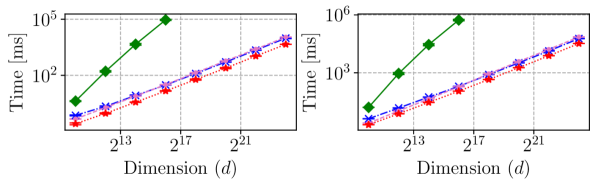
(a) Dimension sweep. Runtime for $s=4,16$.

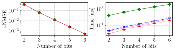
(b) Quantization values sweep. vNMSE and runtime for $d=2^{12}$.

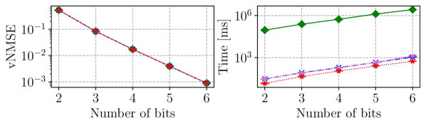
(c) Quantization values sweep. vNMSE and runtime for $d=2^{16}$.

Figure 1: Exact solutions. Sweeping dimension ($d$) and number of quantization values ($s$) for the LogNormal(0,1) distribution.

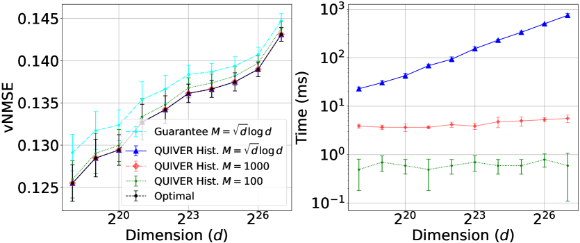
Figure 2: The effect of $M$ on runtime, vNMSE, and the theoretical guarantee for the LogNormal(0,1) distribution and $s=8$.

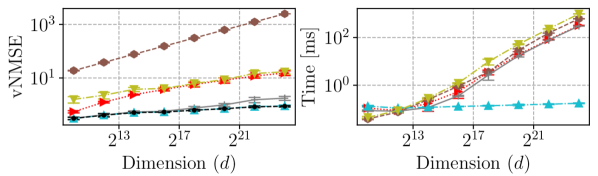
(a) Using $s=4$ quantization values and $M=100$ bins.

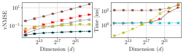
(b) Using $s=16$ quantization values and $M=400$ bins.

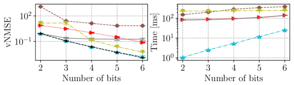
(c) Using dimension $d=2^{22}$ and $M=1000$ bins.

(d) Using dimension $d=2^{22}$ and $s=32$ quantization values.

Figure 3: Approximate solutions. Sweeping $d$, $s$ and the number of bins ($M$) for the LogNormal(0,1) distribution.

Setup.

We implement all algorithms in C++. We use a g4dn.4xlarge AWS EC2 server with custom Intel Cascade Lake CPUs (optimized for ML) with 64 GB RAM and Ubuntu 22.04 OS. All results are averaged over 5 seeds, and presented with error bars.

Distributions.

Here, we present results for the LogNormal distribution and defer to Appendix D results for Normal, Exponential, TruncNorm, and Weibull distributions. As mentioned, these distributions are of interest as they are reported to capture gradients, model weights and activations (see Section 1).

Baselines.

We evaluate our binary search (§4) algorithm, QUIVER and its accelerated version (§5), and compare its MSE and runtime to ZipML (Zhang et al., 2017). For the approximate variant, we evaluate QUIVER (termed QUIVER Hist) with an $M$-sized histogram. We compare it with three approximation variants of ZipML proposed in (Zhang et al., 2017) and the recently proposed ALQ (Faghri et al., 2020). We further discuss these approximations in Appendix B.

Optimal algorithms experiments.

The results are presented in Figure 1. Figure 1(a) shows the runtime for optimally solving the AVQ problem for different dimensions and $s$. As shown, all our solutions are markedly faster than ZipML, which we are unable to run for dimensions $d\geq 2^{17}$ due to its prohibitively large memory requirements. The asymptotic difference ($O(s\cdot d^{2})$ for ZipML, $O(s\cdot d\log d)$ for our Bin-Search algorithm and $O(s\cdot d)$ for QUIVER and its acceleration) is clearly visible in the different slopes on the log-log plot. It is evident that the accelerated version of QUIVER is faster than both Bin-Search and QUIVER. For example, Acc. QUIVER can compute the optimal quantization values for a $1$M-sized vector in under a quarter of a second.

Next, Figure 1(b) and  Figure 1(c) show the vNMSE and speed with respect to the number of bits $b$ (i.e., $s=2^{b}$) for $d=2^{12}$ and $d=2^{16}$. As shown, the vNMSE decays exponentially with $b$ while the runtime increases linearly in $s$. As shown, even for these small dimensions, our algorithms are orders of magnitude faster than ZipML. Also, it is evident that Bin-Search is faster than QUIVER for low dimensions (Figure 1(b)). Again, the accelerated version of QUIVER is faster than both for all evaluated parameters.

Approximate algorithms experiments.

We first run an experiment, whose results are shown in Figure 2, that shows the vNMSE and runtime of QUIVER with different histogram sizes $M$. As shown, the error with $M=\sqrt{d}\log d$ is indeed lower than the theoretical guarantee (Section 6). Interestingly, it shows that with $M=1000$, the error is nearly identical to the Optimal while being significantly faster, and even $M=100$ is not far behind. As a result, we conduct further experiments with $M\in[100,1000]$. Notably, with $M=100$, QUIVER Hist quantizes vectors larger than $133$M coordinates within less than 1 millisecond while being not much worse than the optimum.

The comparison results are presented in Figure 3. It is evident in Figures 3(a) and 3(b) that approximate solutions are significantly faster than exact ones. Also, QUIVER Hist offers both near-optimal vNMSE and the fastest runtime as the dimension increases. As can be seen in Figures 3(c) and 3(d), QUIVER Hist offers these advantages for a different number of quantization values and for a low number of bins.

8 Discussion

We show that computing the optimal (or near-optimal) quantization values can be done on the fly, even for large input vectors, using our algorithms that asymptotically improve the runtime and space complexity of the state of the art. Similarly to previous works (e.g., Zhang et al. (2017)), we assume that the input vector is sorted. If it is not, one can sort the vector, bringing the exact solution complexity to $O(d\log d+s\cdot d)$. In practice, this sorting can be done on the GPU and is rarely the bottleneck; indeed, in Appendix C we measure the time it takes to sort the vector on a T4 GPU, and also to quantize the vector after an AVQ outputs the optimal quantization values.

For example, the sorting and quantization time for a 1$M$-sized vector sums up to only 4ms where the runtime of Accelerated QUIVER is 250ms.

Finally, we note that the histogram solutions do not require the vector to be sorted and the time complexity remains $O(d+s\cdot M)$ even for non-sorted inputs, potentially making them even more appealing compared to the exact ones. Moreover, the histogram calculation is GPU-friendly, and by offloading it to GPU we get that the time complexity of the CPU implementation can reduce to $O(s\cdot M)$, i.e., sublinear in the input vector size.

Acknowlegements:

We thank Wenchen Han for his insightful comments and suggestions.

Appendix A Generalizing Our Algorithms to Weighted Inputs

We now generalize our algorithms for processing sorted weighted inputs $Y=\left\langle(y_{1},w_{1}),\ldots,(y_{n},w_{n})\right\rangle$ (where each entry has value $y_{\ell}$ and weight $w_{\ell}$ and $y_{1}\leq y_{2}\leq\ldots,y_{n}$).

Most of the algorithmic parts, including the Binary Search (Algorithm 2) and QUIVER (Algorithm 3) only require a revised method for computing $C$ in constant time, which is achieved through the modified pre-processing procedure below. The accelerated method (Algorithm 4) needs some $C_{2}$ to be computable in constant time, which is possible for the histogram use case, as we later show.

Pre-processing.

To allow constant time computation of $C$ for weighted inputs we need another auxiliary array. Namely, we define the following:

$$\alpha_{j}={\sum_{(y,w)\in Y_{j}}w}\qquad\ \ \ ,\quad j\in\left\{1,\ldots,n\right\}\ ,$$

$$\beta_{j}={\sum_{(y,w)\in Y_{j}}w\cdot y}\quad\ \ ,\quad j\in\left\{1,\ldots,n\right\}\ ,$$

$$\gamma_{j}={\sum_{(y,w)\in Y_{j}}w\cdot y^{2}}\quad,\quad j\in\left\{1,\ldots,n\right\}\ .$$

Then, we can then write:

$$C [k,j]=\sum_{y_{\ell}\in[y_{k},y_{j}]}w\cdot(y_{j}-y_{\ell})(y_{\ell}-y_{k})$$

$$=\sum_{y_{\ell}\in(y_{k},y_{j}]}w\cdot(y_{j}-y_{\ell})(y_{\ell}-y_{k})$$

$$=y_{j}\cdot y_{k}\cdot\sum_{y_{\ell}\in(y_{k},y_{j}]}w_{\ell}+(y_{j}-y_{k})\cdot\sum_{y_{\ell}\in(y_{k},y_{j}]}w_{\ell}\cdot y_{\ell}$$

$$\qquad\qquad\qquad-\sum_{y_{\ell}\in(y_{k},y_{j}]}w_{\ell}\cdot y_{\ell}^{2}$$

$$=y_{j}\cdot y_{k}\cdot(\alpha_{j}-\alpha_{k})+(y_{j}-y_{k})\cdot(\beta_{j}-\beta_{k})-(\gamma_{j}-\gamma_{k}).$$

Optimal quantization value.

We repeat the analysis for the weighted case. Let us define the sum of weighted variances in the range $[y_{k},y_{j}]$ as a function of $q$, given quantization values at $\left\{y_{k},q,y_{j}\right\}$:

$$Q(q) =\sum_{y_{\ell}\in[y_{k},q]}w_{\ell}\cdot(q-y_{\ell})(y_{\ell}-y_{k})$$

$$+\sum_{y_{\ell}\in(q,y_{j}]}w_{\ell}\cdot(y_{j}-y_{\ell})(y_{\ell}-q).$$

This function is differentiable in $[y_{k},y_{j}]\setminus Y$, and we get:

$$\frac{dQ(q)}{dq}=\sum_{y_{\ell}\in[y_{k},q]}w_{\ell}\cdot(y_{\ell}-y_{k})-\sum_{y_{\ell}\in(q,y_{j}]}w_{\ell}\cdot(y_{j}-y_{\ell}).$$

Similarly, $Q(q)$ is minimized at $u=\inf_{q}(\frac{dQ(q)}{dq}>0)$, where $u\in Y$. Denote by $b^{*}_{k,j}$, where $b^{*}_{k,j}\in\left\{k,\ldots,j\right\}$ the value such that $y_{b^{*}_{k,j}}=u$. Therefore, we require

$$\sum_{\ell=k+1}^{b^{*}_{k,j}}w_{\ell}\cdot(y_{\ell}-y_{k})-\sum_{\ell={b^{*}_{k,j}}+1}^{j}w_{\ell}\cdot(y_{j}-y_{\ell})>0.$$

With some simplifications, this is equivalent to:

$$\sum_{\ell=k+1}^{j}w_{\ell}\cdot y_{\ell}-y_{k}\sum_{\ell=k+1}^{b^{*}_{k,j}}w_{\ell}-y_{j}\sum_{\ell={b^{*}_{k,j}}+1}^{j}w_{\ell}>0$$

$$(\beta_{j}-\beta_{k})-y_{k}(\alpha_{b^{*}_{k,j}}-\alpha_{k})-y_{j}(\alpha_{j}-\alpha_{b^{*}_{k,j}})>0$$

$$\alpha_{b^{*}_{k,j}}>\frac{y_{j}\alpha_{j}-y_{k}\alpha_{k}+(\beta_{j}-\beta_{k})}{y_{j}+y_{k}}.$$

For our histogram use-case (i.e., $n=M+1$), all the weights are integers and they sum up to $d$. We thus find that:

$$\alpha_{b^{*}_{k,j}}=\left\lceil\frac{y_{j}\alpha_{j}-y_{k}\alpha_{k}+(\beta_{j}-\beta_{k})}{y_{j}+y_{k}}\right\rceil,$$

which gives

$${b^{*}_{k,j}}=\alpha^{-1}\left(\left\lceil\frac{y_{j}\alpha_{j}-y_{k}\alpha_{k}+(\beta_{j}-\beta_{k})}{y_{j}+y_{k}}\right\rceil\right).$$

We can therefore compute ${b^{*}_{k,j}}$ in constant time by storing the inverse mapping $\alpha^{-1}:\left\{1,\ldots,d\right\}\to\left\{1,\ldots,M+1\right\}$ explicitly using $O(d)$ space.

Appendix B AVQ Approximation Baselines

In the ZipML paper (Zhang et al., 2017), the authors propose two heuristic methods for improving the runtime. The first heuristic includes calculating the optimal solution on a subset of $X$ called candidate points (CP); they further present an analysis that bounds the error with respect to the maximal difference between consecutive CPs and the maximal number of points in $X$ between consecutive CPs; however, as they do not provide a way to select the CPs, we consider two natural choices: using Uniform CPs, i.e., $\left\{x_{1}+\ell\cdot\frac{x_{d}-x_{1}}{M}\mid\ell\in\left\{0,\ldots,M\right\}\right\}$. This variant is termed ‘ZipML-CP Unif.’ in our evaluation. The second choice of CP is Quantiles, which uses the set $\left\{x_{\left\lfloor 1+\ell\cdot(d-1)/M\right\rfloor}\mid\ell\in\left\{0,\ldots,M\right\}\right\}.$ This variant is termed ‘ZipML-CP Quant.’ in our evaluation.

The second heuristic has a bicretira MSE guarantee: using $2s$ quantization values, it ensures that the MSE is at most twice that of the optimal solution with $s$ quantization values. This variant is termed ‘ZipML 2-Apx’ in our evaluation.

We also compare against ALQ (Faghri et al., 2020), which fits the parameters of a truncated normal distribution to approximate the distribution of the input vector after normalizing it by its norm. It then uses an iterative solution to approximate the optimal quantization values of the fitted distribution up to the desired precision. As suggested by the authors, we use ten iterations, which were shown to converge to the optimal quantization levels for the resulting (truncated normal) distribution.

Appendix C Additional Overheads

We measure the sort and quantize operations using the same EC2 server that is also equipped with an NVIDIA T4 GPU, PyTorch v2.1.2, and CUDA tool kit v12.3. As shown in Figure 4, both operations are fast even for large vectors, despite the usage of a somewhat weak GPU. This specific measurement was done over the LogNormal(0,1) distribution, but the sorting and quantization times are largely independent of the specific distribution and were similar to other tested distributions as well.

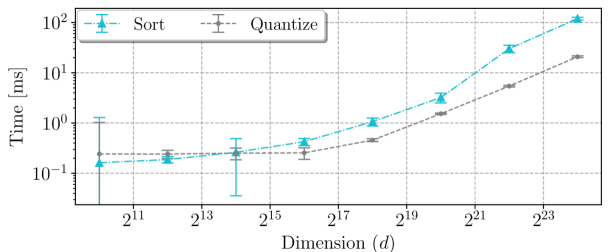
Figure 4: Sort and quantization times vs. $d$ on a T4 GPU.

Appendix D Additional evaluation results

Additional evaluation results of exact solutions.

We provide results for additional input vectors distributions: Normal (Figure 5), Exponential (Figure 6), Truncated Normal (Figure 7), and Weibull (Figure 8). As shown, all follow the same trends in terms of vNMSE, while the runtime is largely independent of the input.

Additional evaluation results of approximate solutions.

Similarly, we show the approximation algorithms evaluation results for the various distributions and $s$ values: LogNormal (Figure 9), Normal (Figure 10), Exponential (Figure 11), Truncated Normal (Figure 12), and Weibull (Figure 13). Once again, the runtime of all algorithms is hardly affected by the input distribution. QUIVER Hist. is always the most accurate and has a near-optimal vNMSE when using a sufficient value for $M$ (e.g., $M\geq 400$) while being markedly faster than all alternatives.

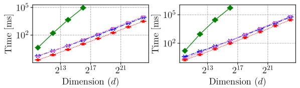
(a) Dimension sweep. Runtime for $s=4,16$.

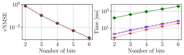
(b) Quantization values sweep. vNMSE and runtime for $d=2^{12}$.

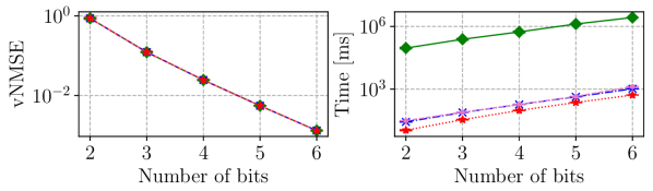
(c) Quantization values sweep. vNMSE and runtime for $d=2^{16}$.

Figure 5: Exact solutions. Sweeping dimension ($d$) and number of quantization values ($s$) for the Normal(0,1) distribution.

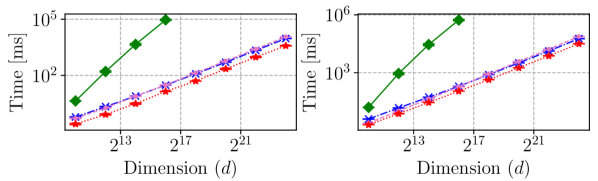
(a) Dimension sweep. Runtime for $s=4,16$.

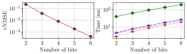
(b) Quantization values sweep. vNMSE and runtime for $d=2^{12}$.

(c) Quantization values sweep. vNMSE and runtime for $d=2^{16}$.

Figure 6: Exact solutions. Sweeping dimension ($d$) and number of quantization values ($s$) for the Exponential(1) distribution.

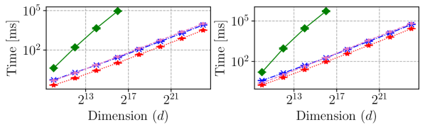
(a) Dimension sweep. Runtime for $s=4,16$.

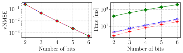
(b) Quantization values sweep. vNMSE and runtime for $d=2^{12}$.

(c) Quantization values sweep. vNMSE and runtime for $d=2^{16}$.

Figure 7: Exact solutions. Sweeping dimension ($d$) and number of quantization values ($s$) for the TruncNorm($\mu=$0,$\sigma^{2}=$1,$a=$-1,$b=$1) distribution.

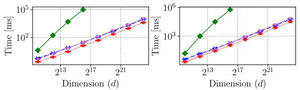
(a) Dimension sweep. Runtime for $s=4,16$.

(b) Quantization values sweep. vNMSE and runtime for $d=2^{12}$.

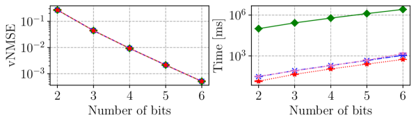
(c) Quantization values sweep. vNMSE and runtime for $d=2^{16}$.

Figure 8: Exact solutions. Sweeping dimension ($d$) and number of quantization values ($s$) for the Weibull(1,1) distribution.

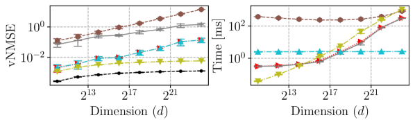
(a) Using $s=64$ quantization values and $M=100$ bins.

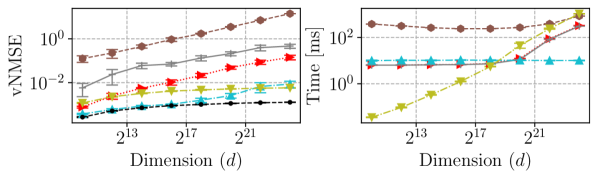
(b) Using $s=64$ quantization values and $M=400$ bins.

(c) Using dimension $d=2^{22}$ and $M=1000$ bins.

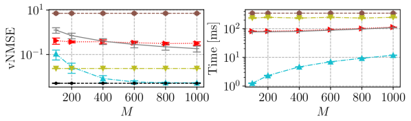
(d) Using dimension $d=2^{22}$ and $s=32$ quantization values.

Figure 9: Approximate solutions. Sweeping $d$, $s$ and the number of bins ($M$) for the LogNormal(0,1) distribution.

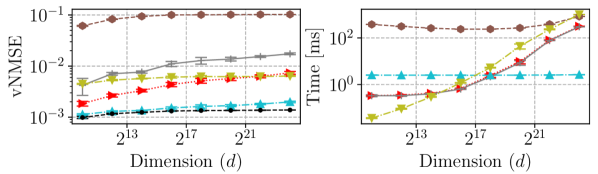
(a) Using $s=64$ quantization values and $M=100$ bins.

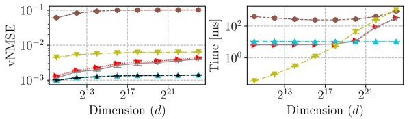
(b) Using $s=64$ quantization values and $M=400$ bins.

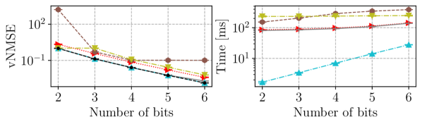
(c) Using dimension $d=2^{22}$ and $M=1000$ bins.

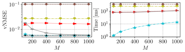
(d) Using dimension $d=2^{22}$ and $s=32$ quantization values.

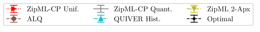
Figure 10: Approximate solutions. Sweeping $d$, $s$ and the number of bins ($M$) for the Normal(0,1) distribution.

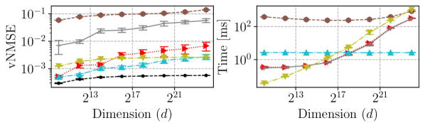
(a) Using $s=64$ quantization values and $M=100$ bins.

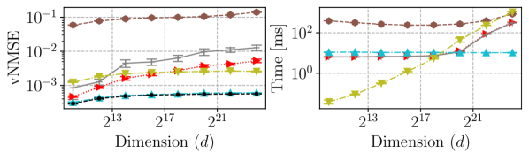
(b) Using $s=64$ quantization values and $M=400$ bins.

(c) Using dimension $d=2^{22}$ and $M=1000$ bins.

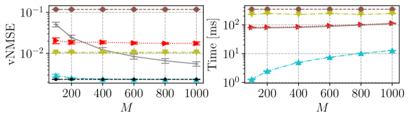
(d) Using dimension $d=2^{22}$ and $s=32$ quantization values.

Figure 11: Approximate solutions. Sweeping $d$, $s$ and the number of bins ($M$) for the Exponential(1) distribution.

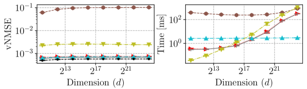
(a) Using $s=64$ quantization values and $M=100$ bins.

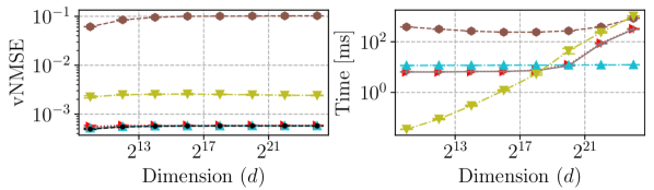
(b) Using $s=64$ quantization values and $M=400$ bins.

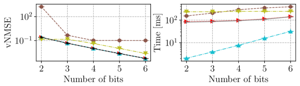
(c) Using dimension $d=2^{22}$ and $M=1000$ bins.

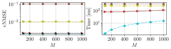
(d) Using dimension $d=2^{22}$ and $s=32$ quantization values.

Figure 12: Approximate solutions. Sweeping $d$, $s$ and the number of bins ($M$) for the TruncNorm($\mu=$0,$\sigma^{2}=$1,$a=$-1,$b=$1) distribution.

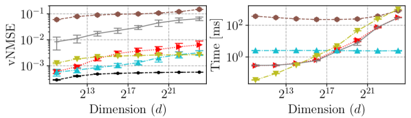
(a) Using $s=64$ quantization values and $M=100$ bins.

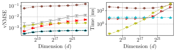
(b) Using $s=64$ quantization values and $M=400$ bins.

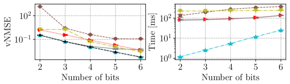
(c) Using dimension $d=2^{22}$ and $M=1000$ bins.

(d) Using dimension $d=2^{22}$ and $s=32$ quantization values.

Figure 13: Approximate solutions. Sweeping $d$, $s$ and the number of bins ($M$) for the Weibull(1,1) distribution.

References

• Alistarh et al. (2017) Alistarh, D., Grubic, D., Li, J., Tomioka, R., and Vojnovic, M. QSGD: Communication-Efficient SGD via Gradient Quantization and Encoding. Advances in Neural Information Processing Systems, 30:1709–1720, 2017.
• Banner et al. (2019) Banner, R., Nahshan, Y., and Soudry, D. Post Training 4-Bit Quantization of Convolutional Networks for Rapid-Deployment. In NeurIPS, 2019.
• Basat et al. (2022) Basat, R. B., Vargaftik, S., Portnoy, A., Einziger, G., Ben-Itzhak, Y., and Mitzenmacher, M. QUIC-FL: Quick Unbiased Compression for Federated Learning. arXiv preprint arXiv:2205.13341, 2022.
• Ben Basat, Ran and Mitzenmacher, Michael and Vargaftik, Shay (2021) Ben Basat, Ran and Mitzenmacher, Michael and Vargaftik, Shay. How to Send a Real Number Using a Single Bit (And Some Shared Randomness). In 48th International Colloquium on Automata, Languages, and Programming (ICALP 2021), volume 198, pp.  25, 2021.
• Caldas et al. (2018) Caldas, S., Konečný, J., McMahan, H. B., and Talwalkar, A. Expanding the Reach of Federated Learning by Reducing Client Resource Requirements. arXiv preprint arXiv:1812.07210, 2018.
• Chmiel et al. (2021) Chmiel, B., Ben-Uri, L., Shkolnik, M., Hoffer, E., Banner, R., and Soudry, D. Neural Gradients are Near-Lognormal: Improved Quantized and Sparse Training. In International Conference on Learning Representations. OpenReview.net, 2021. URL https://openreview.net/forum?id=EoFNy62JGd.
• Dorfman et al. (2023) Dorfman, R., Vargaftik, S., Ben-Itzhak, Y., and Levy, K. Y. DoCoFL: downlink compression for cross-device federated learning. In International Conference on Machine Learning, pp.  8356–8388. PMLR, 2023.
• Faghri et al. (2020) Faghri, F., Tabrizian, I., Markov, I., Alistarh, D., Roy, D. M., and Ramezani-Kebrya, A. Adaptive Gradient Quantization for Data-parallel SGD. Advances in neural information processing systems, 33:3174–3185, 2020.
• Frantar et al. (2023) Frantar, E., Ashkboos, S., Hoefler, T., and Alistarh, D. Optq: Accurate quantization for generative pre-trained transformers. In The Eleventh International Conference on Learning Representations, 2023.
• Fu et al. (2020) Fu, F., Hu, Y., He, Y., Jiang, J., Shao, Y., Zhang, C., and Cui, B. Don’t waste your bits! squeeze activations and gradients for deep neural networks via tinyscript. In International Conference on Machine Learning, pp.  3304–3314. PMLR, 2020.
• Galil & Park (1990) Galil, Z. and Park, K. A Linear-time Algorithm for Concave One-dimensional Dynamic Programming. Information Processing Letters, 33(6):309–311, 1990.
• Horvóth et al. (2022) Horvóth, S., Ho, C.-Y., Horvath, L., Sahu, A. N., Canini, M., and Richtárik, P. Natural Compression for Distributed Deep Learning. In Mathematical and Scientific Machine Learning, pp.  129–141. PMLR, 2022.
• Jeon et al. (2023) Jeon, Y., Lee, C., Park, K., and Kim, H.-y. A Frustratingly Easy Post-Training Quantization Scheme for LLMs. In Proceedings of the 2023 Conference on Empirical Methods in Natural Language Processing, pp.  14446–14461, 2023.
• Konečnỳ & Richtárik (2018) Konečnỳ, J. and Richtárik, P. Randomized Distributed Mean Estimation: Accuracy vs. Communication. Frontiers in Applied Mathematics and Statistics, 4:62, 2018.
• Konečný et al. (2017) Konečný, J., McMahan, H. B., Yu, F. X., Richtárik, P., Suresh, A. T., and Bacon, D. Federated Learning: Strategies for Improving Communication Efficiency. arXiv preprint arXiv:1610.05492, 2017.
• Li et al. (2024) Li, M., Basat, R. B., Vargaftik, S., Lao, C., Xu, K., Tang, X., Mitzenmacher, M., and Yu, M. THC: Accelerating Distributed Deep Learning Using Tensor Homomorphic Compression. In USENIX Symposium on Networked Systems Design and Implementation, 2024.
• Micikevicius et al. (2018) Micikevicius, P., Narang, S., Alben, J., Diamos, G., Elsen, E., Garcia, D., Ginsburg, B., Houston, M., Kuchaiev, O., Venkatesh, G., et al. Mixed Precision Training. In International Conference on Learning Representations, 2018.
• Ramezani-Kebrya et al. (2021) Ramezani-Kebrya, A., Faghri, F., Markov, I., Aksenov, V., Alistarh, D., and Roy, D. M. NUQSGD: Provably Communication-efficient Data-parallel SGD via Nonuniform Quantization. The Journal of Machine Learning Research, 22(1):5074–5116, 2021.
• Safaryan et al. (2020) Safaryan, M., Shulgin, E., and Richtárik, P. Uncertainty Principle for Communication Compression in Distributed and Federated Learning and the Search for an Optimal Compressor. Information and Inference: A Journal of the IMA, 2020.
• Shen et al. (2020) Shen, S., Dong, Z., Ye, J., Ma, L., Yao, Z., Gholami, A., Mahoney, M. W., and Keutzer, K. Q-BERT: Hessian Based Ultra Low Precision Quantization of BERT. In Proceedings of the AAAI Conference on Artificial Intelligence, volume 34, pp.  8815–8821, 2020.
• Sheng et al. (2023) Sheng, Y., Zheng, L., Yuan, B., Li, Z., Ryabinin, M., Chen, B., Liang, P., Ré, C., Stoica, I., and Zhang, C. Flexgen: High-Throughput Generative Inference of Large Language Models With a Single GPU. In International Conference on Machine Learning, pp.  31094–31116. PMLR, 2023.
• Suresh et al. (2017) Suresh, A. T., Felix, X. Y., Kumar, S., and McMahan, H. B. Distributed Mean Estimation With Limited Communication. In International Conference on Machine Learning, pp.  3329–3337. PMLR, 2017.
• Vargaftik et al. (2021) Vargaftik, S., Ben-Basat, R., Portnoy, A., Mendelson, G., Ben-Itzhak, Y., and Mitzenmacher, M. Drive: One-bit Distributed Mean Estimation. Advances in Neural Information Processing Systems, 34:362–377, 2021.
• Vargaftik et al. (2022) Vargaftik, S., Basat, R. B., Portnoy, A., Mendelson, G., Itzhak, Y. B., and Mitzenmacher, M. Eden: Communication-efficient and robust distributed mean estimation for federated learning. In International Conference on Machine Learning, pp.  21984–22014. PMLR, 2022.
• Vladimirova et al. (2018) Vladimirova, M., Arbel, J., and Mesejo, P. Bayesian Neural Networks Become Heavier-Tailed With Depth. In NeurIPS 2018-Thirty-second Conference on Neural Information Processing Systems, pp.  1–7, 2018.
• Ye et al. (2020) Ye, X., Dai, P., Luo, J., Guo, X., Qi, Y., Yang, J., and Chen, Y. Accelerating CNN Training by Pruning Activation Gradients. In European Conference on Computer Vision, pp.  322–338. Springer, 2020.
• Zhang et al. (2017) Zhang, H., Li, J., Kara, K., Alistarh, D., Liu, J., and Zhang, C. ZipML: Training Linear Models with End-to-End Low Precision, and a Little Bit of Deep Learning. In International Conference on Machine Learning, pp.  4035–4043. PMLR, 2017.
• Zhou et al. (2023) Zhou, D., Wang, K., Gu, J., Peng, X., Lian, D., Zhang, Y., You, Y., and Feng, J. Dataset Quantization. In Proceedings of the IEEE/CVF International Conference on Computer Vision, pp.  17205–17216, 2023.