Trustworthiness of Optimality Condition Violation in Inverse Optimal Control Methods Based on the Minimum Principle

Abstract

In this work, we analyze the applicability of Inverse Optimal Control (IOC) methods based on the minimum principle (MP). The IOC method determines unknown cost functions in a single- or multi-agent setting from observed system trajectories by minimizing the so-called residual error, i.e. the extent to which the optimality conditions of the MP are violated with a current guess of cost functions. The main assumption of the IOC method to recover cost functions such that the resulting trajectories match the observed ones is that the given trajectories are the result of an OC problem with a known parameterized cost function structure. However, in practice, when the IOC method is used to identify the behavior of unknown agents, e.g. humans, this assumption cannot be guaranteed. Hence, we introduce the notion of the trustworthiness of the residual error and provide necessary conditions for it to define when the IOC method based on the MP is still applicable to such problems. From the necessary conditions, we conclude that the residual-based IOC method cannot be used to validate OC models for unknown agents. Finally, we illustrate this problem by validating a differential game model for the collision avoidance behavior between two mobile robots with human operators.

I Introduction

Inverse Optimal Control (IOC) methods have gained significant research interest in the last years. Starting with the work of Kalman [1], the question is asked whether a given arbitrary control law is an optimal one, i.e. the solution to an OC problem. To answer this research question, conditions on the system dynamics, control laws and cost functions were proposed under which the given control law is optimal. In recent years, so-called data-based IOC methods arose (see e.g. [2, 3, 4, 5, 6, 7]) which aim at computing unknown cost functions from given system trajectories such that these trajectories are equal to the optimal trajectories resulting from the determined cost functions. In addition, these methods were extended to inverse coupled dynamic optimization problems, i.e. Inverse Dynamic Games (IDG), to determine cost functions for all players such that the given system trajectories are equal to the Nash trajectories resulting from the computed cost functions (see e.g. [8, 9, 10, 11, 12, 13, 14]).

There are two kind of methods to solve such data-based inverse dynamic optimization problems. In direct approaches (see e.g. [8, 14, 7]), the error between the given system trajectories (so-called ground truth (GT)) and trajectories resulting from a current guess of the cost functions is minimized. Here, typically bi-level optimization problems follow. In an upper level, the trajectory error is minimized and in a lower level, a dynamic optimization problem is solved to evaluate the trajectory error in the upper level at a current cost function guess. In indirect approaches (see e.g. [8, 9, 10, 11, 12, 13, 14, 2, 3, 4, 5, 6]), an important assumption, which is made on the given trajectories (see e.g. [8, Definition 6.1], [10, Assumption 1] or [11, Assumption 4.2]), is that they constitute a solution to an OC or DG problem with parameterized cost functions, e.g. running costs are represented by a linear combination of basis functions. Via the indirect method, the unknown parameters of these parameterized cost functions are computed by minimizing violations of optimality conditions, i.e. the so-called residual error, that are fulfilled for the given trajectories and the unknown optimal parameters. The residual error can be defined based on the minimum principle (MP), like in [8, 10, 11, 12, 14, 2, 6], the Hamilton-Jacobi-Bellman equation (see e.g. [9, 13, 3]), the Euler-Lagrange equations (see e.g. [5]) or the Karush-Kuhn-Tucker conditions (see e.g. [4]).

The main assumption of residual-based IOC methods that the given trajectories are optimal w.r.t. known parameterized cost function structures is to be seen critical in practical applications. Data-based IOC approaches are typically used to identify the behavior of an unknown agent or unknown mutually coupled agents from measurement data. Examples can be found in [15, 16, 17, 7] for human movement identification, in [11, 18] for the cooperative steering behavior of two humans or in [19] for the collision avoidance behavior between two birds. In all these cases, the question to be examined is ”are the observed trajectories optimal”, i.e. can an OC/DG model be found to describe the GT data. Since also the cost function structure is unknown, fulfillment of the main assumption cannot be guaranteed. Hence, the crucial question arises if residual-based IOC methods can be used to validate OC/DG models with a postulated cost function structure and if they guarantee usable parameters for a given structure such that the trajectories resulting from the identified models are sufficiently near the best possible trajectories to describe the GT data. For a residual-based IOC method to possess these characteristics, what we call in the following the trustworthiness of the residual error is necessary, i.e. global minimizers of the residual error yield global minimum errors to the GT trajectories. With necessary conditions for the trustworthiness, the applicability of the residual-based IOC method for model validation and determination of usable parameters can be discussed. Until now, research regarding the trustworthiness of residual errors and the possible limitations of corresponding IOC methods for the identification of the behavior of unknown agents is scarce. In literature (see e.g. [11, 13, 14, 6]), only simulations with noisy optimal GT trajectories can be found where the residual error seems to be trustworthy, but conditions or a deeper analysis, e.g. for unknown cost function structures, is missing.

With the contributions in this paper, we close this research gap. Firstly, we define the trustworthiness of the residual error in IOC methods based on the MP. We show that the main assumption of the IOC method (optimality of the given trajectories w.r.t. known cost function structures) is actually a necessary condition for the trustworthiness. Therefore, we conclude that the residual-based IOC method cannot be used in practice to validate OC/DG model assumptions and usable parameters are only determined if a validated cost function structure is already given. Finally, we illustrate this in a practical example by validating a differential game model for the collision avoidance behavior between two mobile robots with human operators. Although we focus on the IOC method based on the MP, we suspect that the results and conclusions generalize to all residual-based IOC methods.

II Inverse Optimal Control based on the Minimum Principle

In this section, we introduce the IDG method based on the MP [8, 10, 11, 14]. For the special case of one player the following DG reduces to an OC problem and the IDG approach to the IOC method in [6].

Let an input-affine dynamic system be defined by

$$\begin{aligned} \dot{\bm{x}}=\bm{f}\left(\bm{x},\bm{u}_{1},\dots,\bm{u}_{N}\right)=\bm{f}_{\bm{x}}(\bm{x})+\sum_{i=1}^{N}\bm{G}_{i}(\bm{x})\bm{u}_{i}\end{aligned}$$ (1)

and $\bm{x}(0)=\bm{x}_{0}$, where $\bm{x}\in\mathbb{R}^{n}$ denotes the system state, $\bm{u}_{i}\in\mathbb{R}^{m_{i}}$ the control variable of player $i\in\mathcal{P}=\{1,\dots,N\}$ and $\bm{x}_{0}$ the initial state at the initial time $t_{0}=0$. Moreover, $\bm{f}_{\bm{x}}:\mathbb{R}^{n}\rightarrow\mathbb{R}^{n}$ and $\bm{G}_{i}:\mathbb{R}^{n}\rightarrow\mathbb{R}^{n\times m_{i}}$ are continuously differentiable w.r.t. $\bm{x}$. Furthermore, let $\bm{u}=\left[\begin{matrix}\bm{u}_{1}^{\top}&\dots&\bm{u}_{N}^{\top}\end{matrix}\right]^{\top}$ and $\bm{u}_{\neg i}=\left[\begin{matrix}\bm{u}_{1}^{\top}&\dots&\bm{u}_{i-1}^{\top}&\bm{u}_{i+1}^{\top}&\dots&\bm{u}_{N}^{\top}\end{matrix}\right]^{\top}$. In the DG, each player $i\in\mathcal{P}$ influences system (1) by applying a control strategy $\bm{u}_{i}(t)=\bm{\gamma}_{i}\left(\bm{x}_{0},t_{0}\right)$ from the set of admissible strategies $\Gamma_{i}$ such that its individual cost function

$$J_{i}=h_{i}(\bm{x}(T))+\int_{0}^{T}g_{i}\left(\bm{x},\bm{u}_{i}\right)\text{d}t$$ (2)

is minimized, where $h_{i}:\mathbb{R}^{n}\rightarrow\mathbb{R}$ denotes the terminal costs and $g_{i}:\mathbb{R}^{n}\times\mathbb{R}^{m_{i}}\rightarrow\mathbb{R}$ the running costs. Furthermore, $h_{i}$ is supposed to be continuously differentiable and convex w.r.t. $\bm{x}$ and $g_{i}(\bm{x},\bm{u}_{i})=q_{i}(\bm{x})+\bm{u}_{i}^{\top}\bm{R}_{i}\bm{u}_{i}$ with $q_{i}:\mathbb{R}^{n}\rightarrow\mathbb{R}$ being continuously differentiable w.r.t. $\bm{x}$ and positive semidefinite and $\bm{R}_{i}$ positive definite. Here, we assume an open-loop (OL) information pattern of the players, i.e. the admissible strategies $\bm{\gamma}_{i}(\bm{x}_{0},t_{0})$ depend only on the initial state and time. In the OL pattern, the strategies are equivalent to the control trajectories $\bm{u}_{i}(t),\forall t\in[0,T]$ applied during the game. Overall, the DG problem is defined by finding $\forall i\in\mathcal{P}$ the optimal control strategy $\bm{\gamma}_{i}^{*}\in\Gamma_{i}$ such that $J_{i}$ is minimized.

We assume a non-cooperative game, i.e. all players minimize their individual cost function (2) regardless of possible negative influences on other players, and that all players act simultaneously. Therefore, the corresponding solution concept are OL Nash equilibria (OLNE). Lemma 1 states the necessary and sufficient conditions to calculate them.

Lemma 1

Let a DG be defined by (1) and (2). Furthermore, let the Hamiltonian functions

$$H_{i}(\bm{\psi}_{i},\bm{x},\bm{u})=g_{i}(\bm{x},\bm{u}_{i})+\bm{\psi}_{i}^{\top}\bm{f}(\bm{x},\bm{u}),\quad\forall i\in\mathcal{P},$$ (3)

where $\bm{\psi}_{i}:[0,T]\rightarrow\mathbb{R}^{n}$ are so-called costate functions, be continuously differentiable and convex w.r.t. $\bm{x}$. If $\bm{\gamma}^{*}=\left[\begin{matrix}{\bm{\gamma}_{1}^{*}(\bm{x}_{0},t_{0})}^{\top}&\dots&{\bm{\gamma}_{N}^{*}(\bm{x}_{0},t_{0})}^{\top}\end{matrix}\right]^{\top}=\bm{u}^{*}(t)$ provides an OLNE with the corresponding state trajectory $\bm{x}^{*}(t)$, the costate functions $\bm{\psi}_{i}(t),\forall i\in\mathcal{P}$ fulfill

$$\dot{\bm{x}}^{*}(t) =\bm{f}\left(\bm{x}^{*}(t),\bm{u}^{*}(t)\right),\quad\bm{x}^{*}(0)=\bm{x}_{0},$$ (4)

$$\bm{0} =\nabla_{\bm{u}_{i}}H_{i}\left(\bm{\psi}_{i}(t),\bm{x}^{*}(t),\bm{u}_{i},\bm{u}_{\neg i}^{*}(t)\right)\big{|}_{\bm{u}_{i}=\bm{u}_{i}^{*}(t)},$$ (5)

$$\dot{\bm{\psi}}_{i}(t) =-\nabla_{\bm{x}}H_{i}(\bm{\psi}_{i}(t),\bm{x},\bm{u}^{*}(t))\big{|}_{\bm{x}=\bm{x}^{*}(t)},$$ (6)

$$\bm{\psi}_{i}(T) =\nabla_{\bm{x}}h_{i}\left(\bm{x}\right)\big{|}_{\bm{x}=\bm{x}^{*}(T)}.$$ (7)

Furthermore, if a set of costate functions $\bm{\psi}_{i}(t),\forall i\in\mathcal{P}$, control $\bm{u}^{*}(t)$ and state trajectories $\bm{x}^{*}(t)$ satisfy (4), (5), (6) and (7), $\bm{u}^{*}(t)$ constitutes an OLNE.

Proof:

Necessity of the conditions (4), (5), (6) and (7) for an OLNE follows from [20, Theorem 6.11] and sufficiency from [21, Theorem 3.2]. ∎

Eqs. (4), (5), (6) and (7) constitute a two-point boundary value problem (TPBVP) with $(N+1)n$ differential equations, $n$ boundary conditions at $t_{0}$ and $Nn$ at $T$. Thus, depending on the concrete application, an OLNE can be found by using numerical methods such as shooting techniques or collocation formulas.

In order to solve the inverse problem to the defined DG only based on (5) and (6), a common approach is to rewrite $h_{i}$ and $g_{i}$ in (2) as linear combination of basis functions: $h_{i}(\bm{x})=\bm{\zeta}_{i}^{\top}\bm{\lambda}_{i}(\bm{x})$ and $g_{i}(\bm{x},\bm{u}_{i})=\bm{\eta}_{i}^{\top}\bm{\mu}_{i}(\bm{x},\bm{u}_{i})$. This yields

$$J_{i}\widehat{=}\int_{0}^{T}\bm{\theta}_{i}^{\top}\bm{\phi}_{i}\left(\bm{x},\bm{u}\right)\text{d}t$$ (8)

with $\bm{\theta}_{i}^{\top}=\left[\begin{matrix}\bm{\eta}_{i}^{\top}&\bm{\zeta}_{i}^{\top}\end{matrix}\right]\in\mathbb{R}^{M_{i}}$ and $\bm{\phi}_{i}^{\top}=\left[\begin{matrix}\bm{\mu}_{i}^{\top}&\dot{\bm{x}}^{\top}\partialderivative{\bm{\lambda}_{i}}{\bm{x}}^{\top}\end{matrix}\right]$.

Now, Assumption 1 is the typical assumption (see e.g. [8, Definition 6.1], [10, Assumption 1] or [11, Assumption 4.2]) made on the GT data to define the IDG Problem 1 for the IDG methods based on the MP.

Assumption 1

Let observed control $\tilde{\bm{u}}_{i}(t),\forall i\in\mathcal{P}$ and state trajectories $\tilde{\bm{x}}(t)$ be given (so-called GT data). Moreover, let these observed trajectories constitute an OLNE of the DG defined by (1) and (8) with $\bm{\theta}_{i}^{*},\forall i\in\mathcal{P}$: $\tilde{\bm{u}}_{i}(t)=\bm{u}_{i}^{*}(t),\forall i\in\mathcal{P}$ and $\tilde{\bm{x}}(t)=\bm{x}^{*}(t)$.

Problem 1

Let Assumption 1 hold. Find (at least) one non-trivial parameter vector $\hat{\bm{\theta}}_{i},\forall i\in\mathcal{P}$ such that

$$\begin{aligned} \tilde{\bm{u}}_{i}(t)&=\arg\min_{\bm{u}_{i}(t)}\int_{0}^{T}\hat{\bm{\theta}}_{i}^{\top}\bm{\phi}_{i}(\bm{x},\bm{u})\text{d}t,\quad\forall i\in\mathcal{P}\\ \text{w.r.t.}&\hphantom{=}\dot{\bm{x}}=\bm{f}(\bm{x},\bm{u}),\bm{x}(0)=\bm{x}_{0}.\end{aligned}$$ (9)

Due to Assumption 1, the given trajectories $\tilde{\bm{u}}(t)$ and $\tilde{\bm{x}}(t)$ fulfill the optimality conditions (4), (5), (6) and (7) with $\bm{\theta}_{i}^{*},\forall i\in\mathcal{P}$. For the inverse problem $\bm{\theta}_{i}^{*}$ is unknown, i.e. we want to find $\forall i\in\mathcal{P}$ parameters $\hat{\bm{\theta}}_{i}$ such that (5) and (6) are satisfied. This can be done by minimizing the extent to which these OLNE conditions are violated w.r.t. $\bm{\theta}_{i},\forall i\in\mathcal{P}$. This extent can be formulated by defining the residual functions $r_{C,i}(\bm{\theta}_{i},\bm{\psi}_{i})=\norm{\nabla_{\bm{u}_{i}}H_{i}(\bm{\theta}_{i},\bm{\psi}_{i})}_{2}^{2}$ and $r_{L,i}(\bm{\theta}_{i},\bm{\psi}_{i})=\norm{\dot{\bm{\psi}}_{i}+\nabla_{\bm{x}}H_{i}(\bm{\theta}_{i},\bm{\psi}_{i})}_{2}^{2}$ for each player $i\in\mathcal{P}$. Minimizing the so-called residual error $\delta_{R,i}$ w.r.t. $\bm{\theta}_{i}$,

$$\min_{\bm{\theta}_{i},\bm{\psi}_{i}}\underbrace{\int_{0}^{T}r_{C,i}(\bm{\theta}_{i},\bm{\psi}_{i})+r_{L,i}(\bm{\theta}_{i},\bm{\psi}_{i})\text{d}t}_{\delta_{R,i}(\bm{\theta}_{i},\bm{\psi}_{i})},$$ (10)

yields $\hat{\bm{\theta}}_{i}$. According to [11, Lemma 4.2], (10) can be rewritten as a quadratic program (QP), which can be solved independently for each player $i\in\mathcal{P}$.

Lemma 2

The residual error optimization (10) is solved by $\hat{\bm{\theta}}_{i}$ and $\hat{\bm{\psi}}_{i}(t)$ if and only if $\hat{\bm{\alpha}}_{i}^{\top}=\left[\begin{matrix}\hat{\bm{\theta}}_{i}^{\top}&\hat{\bm{\psi}}^{\top}_{i}(0)\end{matrix}\right]$ solves

$$\min_{\bm{\alpha}_{i}}\underbrace{\bm{\alpha}_{i}^{\top}\bm{P}_{i}(0)\bm{\alpha}_{i}}_{\delta_{R,i}(\bm{\alpha}_{i})},$$ (11)

where $\bm{P}_{i}(0)$ is symmetric, positive semidefinite and follows from the Riccati differential equation

$$\dot{\bm{P}}_{i}(t)=\left(\bm{P}_{i}(t)\bm{B}_{i}\!+\!\bm{N}_{i}(t)\right)\left(\bm{P}_{i}(t)\bm{B}_{i}\!+\!\bm{N}_{i}(t)\right)^{\top}\!\!-\!\bm{F}^{\top}_{i}(t)\bm{F}_{i}(t)$$ (12)

with $\bm{P}_{i}(T)=\bm{0}$, $\bm{B}_{i}=\left[\begin{matrix}\bm{0}_{n\times M_{i}}&\bm{I}_{n}\end{matrix}\right]^{\top}$, $\bm{N}^{\top}_{i}(t)=\left[\begin{matrix}\partialderivative{\bm{\phi}_{i}(t)}{\bm{x}}^{\top}&\partialderivative{\bm{f}(t)}{\bm{x}}^{\top}\end{matrix}\right]$ and

$$\bm{F}_{i}(t)=\left[\begin{matrix}\partialderivative{\bm{\phi}_{i}(t)}{\bm{x}}^{\top}&\partialderivative{\bm{f}(t)}{\bm{x}}^{\top}\\ \partialderivative{\bm{\phi}_{i}(t)}{\bm{u}_{i}}^{\top}&\partialderivative{\bm{f}(t)}{\bm{u}_{i}}^{\top}\end{matrix}\right].$$ (13)

Proof:

The result follows from [11, Lemma 4.1] and [11, Lemma 4.2]. ∎

With Lemma 2, potential solutions $\hat{\bm{\theta}}_{i}$ to Problem 1 can be found by solving the convex QP (11) with some additional constraints to avoid the trivial solution $\bm{\theta}_{i}=\bm{0}$, e.g. $\theta_{i,1}=1$. Problem 1 aims at finding parameters $\hat{\bm{\theta}}_{i}$ such that the error between the GT $\tilde{\bm{u}}(t)$ and $\tilde{\bm{x}}(t)$ and the estimated trajectories $\hat{\bm{u}}(t)$ and $\hat{\bm{x}}(t)$ vanishes. This trajectory error can for example be quantified by the normalized sum of absolute errors (NSAE) of the state $\delta_{T}^{\bm{x}}(\hat{\bm{\theta}})$ and controls $\delta_{T}^{\bm{u}}(\hat{\bm{\theta}})$:

$$\delta_{T}^{\bm{x}}(\bm{\theta}) =\sum_{j=1}^{n}\frac{1}{\max_{k}\absolutevalue{\tilde{x}_{j}^{(k)}}}\sum_{k=1}^{K}\absolutevalue{\tilde{x}_{j}^{(k)}-x_{j}^{(k)}\big{|}_{\bm{\theta}}},$$ (14)

$$\delta_{T}^{\bm{u}}(\bm{\theta}) =\sum_{i=1}^{N}\sum_{j=1}^{m_{i}}\frac{1}{\max_{k}\absolutevalue{\tilde{u}_{i,j}^{(k)}}}\sum_{k=1}^{K}\absolutevalue{\tilde{u}_{i,j}^{(k)}-u_{i,j}^{(k)}\big{|}_{\bm{\theta}}},$$ (15)

where $\bm{u}(t)\big{|}_{\bm{\theta}}$ is the OLNE of the DG (1), (8) with $\bm{\theta}$ and $\bm{x}(t)\big{|}_{\bm{\theta}}$ the corresponding state trajectory. Now, Lemma 3 yields sufficient conditions such that a global minimizer $\hat{\bm{\theta}}$ of the residual error $\delta_{R}(\bm{\alpha})=\sum_{i=1}^{N}\delta_{R,i}(\bm{\alpha}_{i})$ (10) solves Problem 1 and thus, yields the global minimum trajectory error $\delta_{T}(\hat{\bm{\theta}})=\delta_{T}^{\bm{x}}(\hat{\bm{\theta}})+\delta_{T}^{\bm{u}}(\hat{\bm{\theta}})=0$.

Lemma 3

Let $\bar{\bm{P}}_{i}$ follow from $\bm{P}_{i}(0)$ by deleting the first row and column. Furthermore, let $\bar{\bm{p}}_{i}$ be the first column of $\bm{P}_{i}(0)$ without the first element and $\bar{\bm{P}}^{+}_{i}$ the pseudoinverse of $\bar{\bm{P}}_{i}$. Let the singular value decomposition of $\bar{\bm{P}}_{i}$ be given by $\bar{\bm{P}}_{i}=\bm{U}_{i}\bm{\Sigma}_{i}\bm{U}_{i}^{\top}$ with

$$\bm{U}_{i}=\left[\begin{matrix}\bm{U}_{i}^{11}&\bm{U}_{i}^{12}\\ \bm{U}_{i}^{21}&\bm{U}_{i}^{22}\end{matrix}\right],$$ (16)

where $\bm{U}_{i}^{11}\in\mathbb{R}^{(M_{i}-1)\times r_{i}}$, $\bm{U}_{i}^{12}\in\mathbb{R}^{(M_{i}-1)\times(M_{i}+n-1-r_{i})}$, $\bm{U}_{i}^{21}\in\mathbb{R}^{n\times r_{i}}$, $\bm{U}_{i}^{22}\in\mathbb{R}^{n\times(M_{i}+n-1-r_{i})}$ and $r_{i}$ is the rank of $\bar{\bm{P}}_{i}$. If Assumption 1 holds and $r_{i}=M_{i}+n-1$ or $\bm{U}_{i}^{12}=\bm{0}$ holds $\forall i\in\mathcal{P}$, $\hat{\bm{\theta}}_{i}=c_{i}\bm{\theta}_{i}^{*}$, $\forall i\in\mathcal{P}$ with $c_{i}\in\mathbb{R}_{>0}$ and hence, the parameters $\hat{\bm{\theta}}_{i}$ solve Problem 1.

Proof:

From [10, Theorem 2], all solutions $\hat{\bm{\theta}}_{i}$ of (11) are unique up to a scaling factor $c_{i}\in\mathbb{R}_{>0}$ if $r_{i}=M_{i}+n-1$ or $\bm{U}_{i}^{12}=\bm{0}$. Furthermore, since Assumption 1 holds and the MP conditions are necessary, for all global minimizers of (11) $\delta_{R}=0$ holds and $\bm{\theta}_{i}^{*}$ is one of them. Thus, we find a $c_{i}$ such that $\hat{\bm{\theta}}_{i}=c_{i}\bm{\theta}_{i}^{*}$. Lastly, all parameters $\hat{\bm{\theta}}_{i}=c_{i}\bm{\theta}_{i}^{*}$ yield $\hat{\bm{u}}(t)=\tilde{\bm{u}}(t)$ and $\hat{\bm{x}}(t)=\tilde{\bm{x}}(t)$. ∎

As explained in Section I, Assumption 1 cannot be guaranteed in applications where the behavior of unknown agents needs to be identified. The parameterized cost function structures, i.e. the basis functions $\bm{\phi}_{i}$ in (8), are unknown as well. Hence, in practice, we first need to postulate such a cost function structure and validate it based on measurement data by computing the best possible parameters $\hat{\bm{\theta}}$ regarding the trajectory error $\delta_{T}$ with an IOC method. If a cost function structure is found guaranteeing a sufficiently small $\delta_{T}$ ($\delta_{T}=0$ is unrealistic in most applications), an IOC method is needed that determines usable parameters for the cost function structure, i.e. the resulting trajectories yield a sufficiently small $\delta_{T}$ although $\delta_{T}=0$ is not possible. Remarkably, since direct IOC methods minimize the trajectory error to the GT data, e.g. $\delta_{T}$, they fulfill these characteristics by definition. For a residual-based IOC method, the trustworthiness of the residual error, e.g. $\delta_{R}$ for the MP-based method, is necessary which we define in the following section. Since the conditions in Lemma 3 are only sufficient for the trustworthiness of $\delta_{R}$, we provide necessary conditions to discuss if Assumption 1, i.e. knowing the cost function structure/basis functions, is really a necessary condition for it. Then, the applicability of the residual-based IOC method for model validation and estimation of usable parameters can be assessed.

III Necessary Conditions for the Trustworthiness of Optimality Condition Violation

Definition 1

The residual error $\delta_{R}(\bm{\alpha})$ (10) of the IOC method based on the MP is called trustworthy if a global minimizer $\hat{\bm{\theta}}^{\text{MP}}$ of $\delta_{R}(\bm{\alpha})$ is (approximately) a global minimizer $\hat{\bm{\theta}}^{\text{BL}}$ of $\delta_{T}(\bm{\theta})=\delta_{T}^{\bm{x}}(\bm{\theta})+\delta_{T}^{\bm{u}}(\bm{\theta})$ (14), (15): $\norm{\hat{\bm{\theta}}^{\text{MP}}-\hat{\bm{\theta}}^{\text{BL}}}<\epsilon$ with $\epsilon$ sufficiently small.

In order to illustrate the trustworthiness of the residual error, we first look at the case where the conditions of Lemma 3 hold, which are sufficient for the trustworthiness of $\delta_{R}$ with $\epsilon=0$. Let the OC problem of a single-player double integrator be defined by the dynamic system

$$\dot{\bm{x}}=\left[\begin{matrix}0&1\\ 0&0\end{matrix}\right]\bm{x}+\left[\begin{matrix}0\\ 1\end{matrix}\right]u,\quad\bm{x}(0)=\left[\begin{matrix}1\\ -1\end{matrix}\right]$$ (17)

and the cost function

$$J_{i}=\int_{0}^{6}\left[\begin{matrix}1&2&1\end{matrix}\right]\left[\begin{matrix}u^{2}&x_{1}^{2}&x_{2}^{2}\end{matrix}\right]^{\top}\text{d}t.$$ (18)

Solving the OC problem given by (17) and (18) yields the GT trajectories $\tilde{\bm{x}}(t)$ and $\tilde{u}(t)$ that are optimal w.r.t. $\bm{\theta}^{*}=\left[\begin{matrix}1&2&1\end{matrix}\right]^{\top}$. Now, by stating the QP of Lemma 2 with equality constraint $\theta_{1}=1$, the IOC problem (Problem 1 with $N=1$) is tried to be solved. By evaluating the residual $\delta_{R}(\bm{\alpha})$ and the trajectory error $\delta_{T}(\bm{\theta})$ for varying $\theta_{2}$-values by setting $\theta_{1}=1$, $\theta_{3}=\theta_{3}^{*}$ and $\bm{\psi}(0)=\bm{\psi}^{*}(0)$, Fig. 1 results. Here, the residual error $\delta_{R}$ is trustworthy in the sense of Definition 1 with $\epsilon=0$: the global minimizers of $\delta_{R}$ are global minimizers of $\delta_{T}$ as well and since for the global minimum trajectory error $\delta_{T}=0$ holds, they solve Problem 1.

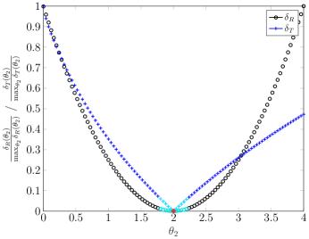
Figure 1: Normalized residual $\delta_{R}$ and trajectory error $\delta_{T}$ for the double integrator example system when $\delta_{R}$ is trustworthy in the sense of Definition 1. For both error types, the 10 smallest values are marked in cyan except that minimum value which is marked in red.

In order to relax the conditions in Lemma 3, Proposition 1 introduces necessary conditions for the trustworthiness of $\delta_{R}$.

Proposition 1

If the residual error $\delta_{R}(\bm{\alpha})$ (10) is trustworthy in the sense of Definition 1, the following conditions hold:

1. The optimality conditions used to derive $\delta_{R}$, i.e. in case of the IOC method from Section II (4), (5), (6) and (7) derived from the MP, are necessary and sufficient for the assumed OC/DG model.

2. The basis functions $\bm{\phi}_{i},\forall i\in\mathcal{P}$, which yield the smallest possible trajectory error $\delta_{T}$, are known.

3. The trivial solution ($\bm{\theta}_{i}=\bm{0}$) of the minimization of $\delta_{R}(\bm{\alpha})$ is omitted, e.g. by introducing suitable constraints.

Proof:

Regarding the first condition, suppose the GT trajectories $\tilde{\bm{x}}(t)$ and $\tilde{\bm{u}}(t)$ are indeed optimal w.r.t. $\bm{\phi}_{i},\forall i\in\mathcal{P}$ and $\bm{\theta}^{*}$. If the optimality conditions are not necessary, a global minimum of $\delta_{R}$ at $\bm{\theta}^{*}$ cannot be guaranteed, although $\delta_{T}=0$. If the optimality conditions are necessary but not sufficient, the residual error is zero when the GT trajectories are only candidates for an optimal solution. Hence, the trajectories that are indeed optimal w.r.t. the determined $\hat{\bm{\theta}}$ can be different: $\delta_{R}=0$ but $\delta_{T}>0$.

The second condition is proofed by a counterexample based on the single-player double integrator. Suppose the basis functions $\bm{\phi}(\bm{x},u)=\left[\begin{matrix}u^{2}&x_{1}^{2}&x_{2}^{2}\end{matrix}\right]^{\top}$, which yield the smallest possible trajectory error, i.e. $\delta_{T}=0$, are unknown and the IOC problem is tried to be solved with $\bm{\phi}(\bm{x},u)=\left[\begin{matrix}u^{2}&x_{2}^{2}\end{matrix}\right]^{\top}$ ($\bm{\theta}=\left[\begin{matrix}\theta_{1}&\theta_{3}\end{matrix}\right]^{\top}$) instead. Fig. 2 shows the residual $\delta_{R}$ and the trajectory error $\delta_{T}$ for varying $\theta_{3}$-values ($\theta_{1}=1$ for both errors and $\bm{\psi}(0)=\bm{\psi}^{*}(0)$ for $\delta_{R}$). The global minima of both error types differ clearly, i.e. $\epsilon\gg 0$. In order to assess if $\epsilon$ can maybe still be seen as sufficiently small in this case, we compare the state and control trajectories of the GT ($\tilde{\bm{x}}(t)$, $\tilde{u}(t)$), the trajectories resulting from the global minimizer $\hat{\bm{\theta}}^{\text{MP}}$ of $\delta_{R}$ ($\hat{\bm{x}}^{\text{MP}}(t)$, $\hat{u}^{\text{MP}}(t)$) and the trajectories resulting from the global minimizer $\hat{\bm{\theta}}^{\text{BL}}$ of $\delta_{T}$ ($\hat{\bm{x}}^{\text{BL}}(t)$, $\hat{u}^{\text{BL}}(t)$) in Fig. 3. Especially, by comparing the state trajectories $\hat{\bm{x}}^{\text{MP}}(t)$ and $\hat{\bm{x}}^{\text{BL}}(t)$, it can be concluded that $\epsilon$ is not sufficiently small in this case since they do not even show similar trends which makes an OC model with $\hat{\bm{\theta}}^{\text{MP}}$ significantly less useful as with $\hat{\bm{\theta}}^{\text{BL}}$.

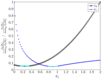
Figure 2: Normalized residual $\delta_{R}$ and trajectory error $\delta_{T}$ for the double integrator system when $\delta_{R}$ is not trustworthy.

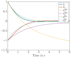
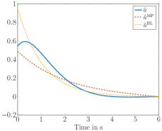
Figure 3: State and control trajectories of the GT (solid lines), the trajectories resulting from the global minimizer $\hat{\bm{\theta}}^{\text{MP}}$ of $\delta_{R}$ (dashed lines) and the trajectories resulting from the global minimizer $\hat{\bm{\theta}}^{\text{BL}}$ of $\delta_{T}$ (dotted lines) for the double integrator system when $\delta_{R}$ is not trustworthy.

With the third condition, the global minimizer $\bm{\alpha}=\bm{0}$ of $\delta_{R}$ is omitted since it yields $\delta_{T}>0$. ∎

Since Proposition 1 provides necessary conditions for the trustworthiness of the residual error. We can make the following conclusions regarding the application of the residual-based IOC method for the identification of unknown agents.

Remark 1

If the residual error $\delta_{R}$ is not trustworthy in the sense of Definition 1, we cannot make any kind of conclusion from the global minimizers of $\delta_{R}$ for the global minimum values of $\delta_{T}$. Regardless of $\delta_{T,\delta_{R,\min}}$ achieved with the global minimizer $\hat{\bm{\theta}}^{\text{MP}}$, $\delta_{T,\min}\approx 0$ or $\delta_{T,\min}\gg 0$ is possible for the global minimum trajectory error.

Since knowing the cost function structure (see condition $2$ in Proposition 1) is a necessary condition for the trustworthiness of $\delta_{R}$ and since trustworthiness of $\delta_{R}$ is necessary to make conclusions regarding $\delta_{T}$ (see Remark 1), an OC/DG model and its postulated cost function structure cannot be validated with the residual-based IOC approach.

Remark 2

The residual-based IOC method based on the MP cannot be used to validate an OC/DG model with a postulated cost function structure, e.g. set of basis functions.

Although the residual-based IOC method cannot be used for model validation for the behavior of unknown agents, the necessary conditions of Proposition 1 highlight that it can still provide usable parameters that yield trajectories with a sufficiently small $\delta_{T}$, even when Assumption 1 does not hold.

Remark 3

If an OC/DG model is validated, e.g. with a direct IOC approach, such that the corresponding cost function structure guarantees the smallest possible trajectory error, an approximate match (cf. Definition 1) of the global minimizers of $\delta_{R}$ and $\delta_{T}$ occurs.

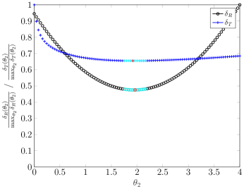
Figure 4: Normalized residual $\delta_{R}$ and trajectory error $\delta_{T}$ for the double integrator system when $\delta_{R}$ is trustworthy but the minimum values are non-zero.

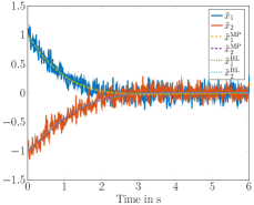
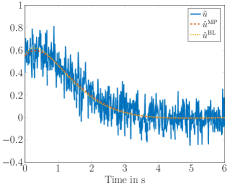
Figure 5: State and control trajectories of the GT, the trajectories resulting from the global minimizer $\hat{\bm{\theta}}^{\text{MP}}$ and the trajectories resulting from the global minimizer $\hat{\bm{\theta}}^{\text{BL}}$ for the double integrator system when $\delta_{R}$ is trustworthy but the minimum values are non-zero.

In order to illustrate Remark 3, we look at the double integrator system (17), (18) and define as GT data the OC solution with $\bm{\theta}^{*}$ but add Gaussian noise: $\tilde{\bm{x}}(t)=\bm{x}^{*}(t)+\bm{\varepsilon}_{1}(t)$, $\tilde{u}(t)=u^{*}(t)+\varepsilon_{2}(t)$ ($\bm{\varepsilon}_{1}(t)\sim\mathcal{N}(\bm{0},0.1^{2}\bm{I})$, $\varepsilon_{2}(t)\sim\mathcal{N}(0,0.1^{2})$). Here, we can assume that the given $\bm{\phi}$ are still the best possible basis functions regarding $\delta_{T}$. Fig. 4 shows the normalized $\delta_{R}$ (with $\theta_{1}=1$, $\theta_{3}=\theta_{3}^{*}$ and $\bm{\psi}(0)=\bm{\psi}^{*}(0)$) and $\delta_{T}$ (with $\theta_{1}=1$ and $\theta_{3}=\theta_{3}^{*}$) regarding different $\theta_{2}$-values. Although Assumption 1 does not hold and an exact match with the GT trajectories ($\delta_{T}=0$) is not possible, the global minimizers of $\delta_{R}$ and $\delta_{T}$ match approximately and trustworthiness of $\delta_{R}$ follows since very similar trajectories for $\hat{\bm{\theta}}^{\text{MP}}$ and $\hat{\bm{\theta}}^{\text{BL}}$ (see Fig. 5) are observed. This explains the results in literature with noisy GT trajectories (see e.g. [11, 13, 14, 6]). The counterexample in the proof of Proposition 1, where the trajectory error $\delta_{T,\min}$ at $\hat{\bm{\theta}}^{\text{BL}}$ in Fig. 3 could still be considered as sufficiently small for some applications, highlights the importance to know the best possible basis functions regarding $\delta_{T}$. For the counterexample, there are basis functions leading to smaller trajectory errors and therefore, the minimizers of both error types do not match sufficiently in Fig. 2.

Remark 3 can be beneficial in practice. Whereas validating a model assumption, e.g. for human movements, can typically be performed offline, applications of validated models often require fast or even real-time parameter identification, for example to adapt prediction models for human movements to different persons or changes in their characteristics. The high computation times of direct IOC approaches [14] can be tolerated in offline model validation but hinder such fast/real-time parameter identifications, which however are possible with residual-based methods [9].

We strongly suspect that Definition 1, Proposition 1, Remark 2 and Remark 3 generalize to residual errors derived in IOC methods based on other optimality conditions.

IV Practical Example: Identification of Multi-Agent Collision Avoidance Behavior

In this section, we illustrate the consequences of Remark 2 by analyzing the validity of a differential game model to describe the collision avoidance behavior between two humans driving mobile robots in a simulation environment with different IOC methods.

IV-A Differential Game Model for Multi-Agent Collision Avoidance between Mobile Robots with Human Operators

The dynamics of each robot $i\in\mathcal{P}=\{1,2\}$ are given by $\dot{\bm{x}}_{i}=\bm{u}_{i}$, where $x_{i,1}$ denotes the x-position and $x_{i,2}$ the y-position of robot $i$. This yields the complete system dynamics $\dot{\bm{x}}=\left[\begin{matrix}\dot{\bm{x}}^{\top}_{1}&\dot{\bm{x}}^{\top}_{2}\end{matrix}\right]^{\top}=\bm{u}$. The individual cost function of each human operator $i\in\mathcal{P}$ is modeled by (8) where the basis functions $\bm{\phi}_{i}(\bm{x},\bm{u})$ follow from

$$\bm{\lambda}_{i}(\bm{x}(T)) =\big{[}(x_{i,1}(T)-x_{i,T,1})^{2}\,\,\,(x_{i,2}(T)-x_{i,T,2})^{2}\big{]}^{\top},$$ (19)

$$\bm{\mu}_{i}(\bm{x},\bm{u}_{i}) =\big{[}u_{i,1}^{2}\,\,\,u_{i,2}^{2}\,\,\,(x_{i,1}-x_{i,T,1})^{2}\,\,\,(x_{i,2}-x_{i,T,2})^{2}$$

$$\hphantom{=}\norm{\bm{x}_{i}-\bm{x}_{j}}^{-1}_{2}\,\,\,\norm{\bm{x}_{i}-\bm{x}_{j}}^{-2}_{2}\big{]}^{\top}$$ (20)

with $j\in\mathcal{P}$ but $j\neq i$. Moreover, the starting positions are given by $\bm{x}_{0}=\left[\begin{matrix}-1\,\text{m}&-0.5\,\text{m}&1\,\text{m}&0\,\text{m}\end{matrix}\right]^{\top}$ and the displayed target points by $\bm{x}_{T}=\left[\begin{matrix}1\,\text{m}&1\,\text{m}&-1\,\text{m}&0\,\text{m}\end{matrix}\right]^{\top}$.

Firstly, we apply the IOC method based on the MP to GT trajectories computed by the DG model with $T=5\,\text{s}$, $\bm{\theta}^{*}_{1}=\left[\begin{matrix}1&4&0&0&0.2&0&100&100\end{matrix}\right]^{\top}$ and $\bm{\theta}^{*}_{2}=\left[\begin{matrix}1&1&0&0&0.2&0&100&100\end{matrix}\right]^{\top}$: $\tilde{\bm{x}}(t)=\bm{x}^{*}(t)$ and $\tilde{\bm{u}}(t)=\bm{u}^{*}(t)$. Due to rewriting the terminal costs in the integrand of $J_{i}$ (cf. (8)), the MP conditions are not sufficient anymore. Hence, the first condition in Proposition 1 is not fulfilled and by computing $\hat{\bm{\theta}}$ with the QP (11) with constraints $\theta_{1,1}=\theta_{2,1}=1$, $\delta_{R,\min}\approx 1.0\cdot 10^{-7}$ and $\delta_{T,\delta_{R,\min}}\approx 2.8\cdot 10^{3}$ follows at $\hat{\bm{\theta}}^{\text{MP}}$, although $\delta_{T,\min}\approx 0$ is possible. Therefore, $\theta_{1,7}\geq 500$, $\theta_{1,8}\geq 500$, $\theta_{2,7}\geq 500$ and $\theta_{2,8}\geq 500$ are used as additional constraints since the QP (11) shows global minimizers independently from the choice of these parameters. However, they need to be sufficiently large such that the DG solution reaches the target points. With the additional constraints, $\delta_{R,\min}\approx 2.8\cdot 10^{-3}$ and $\delta_{T,\delta_{R,\min}}\approx 12.6$ result.

IV-B Study Design

We conducted a simulation study where two humans controlled each a holonomic robot platform with a Playstation 4 controller in the x-y-plane in a Gazebo simulation (cf. Fig. 6). The task for both humans was to drive its robot in a given maximum time horizon of $5\,\text{s}$ from the starting position $\bm{x}_{i,0}$ to the displayed target point $\bm{x}_{i,T}$ (cross in the same color as the robot, yellow for robot $1$ and purple for robot $2$, see Fig. 6) while avoiding collision to the other robot and the test field bounds. The target point was considered as reached if it was inside the rectangular robot ($0.33\,\text{m}\times 0.31\,\text{m}$). A mutual visual starting signal for both players was given via the graphical user interface. Communication between the participants was prohibited before and during the experiment. The collision avoidance experiment was conducted with four groups with two participants each.

Figure 6: Screenshot of the simulation study to analyze the collision avoidance behavior between two humans.

Motivated by OC models for human movements (see e.g. [17, 7]), we hypothesize that the observed behavior can be described by an OLNE. The model assumption is checked by applying data-based IOC methods to the observed GT data. Before the actual collision avoidance experiment between both participants, a familiarization phase was implemented for each participant where the participant had to drive to $10$ arbitrary, successively displayed target points. Then, each group performed $10$ trials of the collision avoidance experiment as training phase to learn the other player’s behavior and then, $10$ trials to collect the GT data. The center of the robot was defined as $\bm{x}_{i}$ and its position was recorded with $50\,\text{Hz}$. The corresponding control signal $\bm{u}_{i}$ follows from numerical differentiation and a cubic spline smoothing. The start time $t_{0}$ of the DG model of one trial was defined as the first point in time where for one robot $\norm{\bm{u}_{i}}_{2}>0.15\,\frac{\text{m}}{\text{s}}$ holds and the final time $T$ as the first point in time where $\norm{\bm{u}_{i}}_{2}<0.1\,\frac{\text{m}}{\text{s}},\forall i\in\mathcal{P}$. Finally, $26$ valid trials result where no collisions occurred and the target points are reached at the final time $T$. For the valid trials, the model Assumption 2 is suggested.

Assumption 2

The collision avoidance behavior between two mobile robots with human operators can be described by an OLNE.

In order to validate Assumption 2, the GT trajectories $\tilde{\bm{x}}(t)$, $\tilde{\bm{u}}(t)$ of each trial are used to compute parameters $\hat{\bm{\theta}}$. The residual-based IOC method yields $\hat{\bm{\theta}}^{\text{MP}}$ at the global minimum residual error $\delta_{R,\min}$ and the direct bi-level-based method minimizing $\delta_{T}$ with the pattern search algorithm of the Matlab environment (same constraints used as for the QP of the residual-based optimization, see Section IV-A) $\hat{\bm{\theta}}^{\text{BL}}$. For each trial, $\bm{x}_{T}$ of the DG model is set to $\bm{x}_{T}=\tilde{\bm{x}}(T)$, where $T$ is the game time horizon determined for each trial based on the absolute velocity thresholds defined before. Afterwards, the trajectory errors $\delta_{T,\delta_{R,\min}}$ and $\delta_{T,\min}$ achieved with $\hat{\bm{\theta}}^{\text{MP}}$ and $\hat{\bm{\theta}}^{\text{BL}}$, respectively, can be compared to illustrate the problem resulting from Remark 2. It is not guaranteed that the proposed $\bm{\phi}_{i}$ are the best possible basis functions. Then, $\delta_{T,\min}$ is used to evaluate Assumption 2. We reject the assumption if for the maximum $\delta_{T,\min}\geq 250$ (threshold qualitatively derived from Fig. 7) holds.

IV-C Study Results

TABLE I: IOC results for the five best and the five worst trials according to $\delta_{T,\min}$.

Group	Trial Number	$\delta_{R,\min}$	$\delta_{T,\delta_{R,\min}}$	$\delta_{T,\min}$
$1$	$14$	$23.6$	$353.2$	$249.8$
$2$	$15$	$30.3$	$1.2\cdot 10^{3}$	$257.6$
$4$	$16$	$1.1\cdot 10^{3}$	$1.3\cdot 10^{3}$	$269.5$
$1$	$17$	$42.5$	-	$302.8$
$4$	$11$	$252.0$	-	$314.3$
$2$	$12$	$178.0$	-	$558.3$
$4$	$17$	$801.0$	-	$574.4$
$3$	$13$	$322.4$	$5.0\cdot 10^{16}$	$601.5$
$3$	$20$	$18.5$	-	$730.5$
$3$	$18$	$2.1\cdot 10^{3}$	-	$776.5$

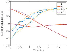
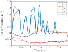
Figure 7: State and control trajectories of the GT and the direct bi-level-based identification for group $2$/trial $15$.

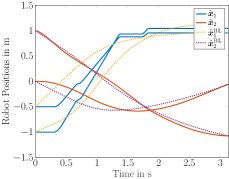
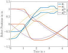
Figure 8: State trajectories of the GT and the bi-level-based identification for group $2$/trial $17$ ($\delta_{T,\min}\approx 434.8$) and group $4$/trial $17$ ($\delta_{T,\min}\approx 574.4$).

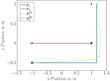
Figure 9: State trajectories and paths of the GT and the direct bi-level-based identification for group $3$/trial $18$.

Table I shows the achieved results of the IOC evaluation described in Section IV-B. The trials are sorted according to $\delta_{T,\min}$ and for clarity, only the five best and five worst trials are shown. Except for group $1$/trial $14$, in all cases $\delta_{T,\delta_{R,\min}}$ and $\delta_{T,\min}$ differ by at least one order of magnitude and in $19$ trials an OLNE cannot even be computed with the parameters $\hat{\bm{\theta}}^{\text{MP}}$ (see missing values for $\delta_{T,\delta_{R,\min}}$ in Table I). This highlights that the residual error is not trustworthy in this practical example due to the unknown optimal basis function configuration. Thus, the residual-based IOC method is not suitable to evaluate Assumption 2 or to provide usable parameters until the best possible basis function configuration is found by a direct IOC approach. The minimum, mean and maximum computation times for $\hat{\bm{\theta}}^{\text{MP}}$ are $0.33\,\text{s}$, $0.55\,\text{s}$ and $1.19\,\text{s}$, respectively. In contrast, the minimum, mean and maximum computation times for $\hat{\bm{\theta}}^{\text{BL}}$ are $2.30\cdot 10^{3}\,\text{s}$, $4.41\cdot 10^{3}\,\text{s}$ and $6.67\cdot 10^{3}\,\text{s}$, respectively, and thus, nearly four orders of magnitude higher.

By evaluating $\delta_{T,\min}$ for the valid trials, Assumption 2 needs to be rejected since $\delta_{T,\min}<250$ was not achieved for any trial. This threshold is qualitatively defined based on the result for group $2$ and its trial $15$ (cf. Fig. 7). The GT control trajectory of the first robot $\tilde{\bm{u}}_{1}(t)$ cannot be described with the DG model. Thus, a trajectory error $\delta_{T,\min}\approx 250$ cannot be sufficiently small to accept the model assumption. In simulation (see Section IV-A), only $\delta_{T,\min}\approx 13$ guarantees a perfect match between predicted and GT trajectories.

IV-D Discussion

The main reason for the relative high trajectory errors, follows from the GT control trajectories. Like in Fig. 7 for $\tilde{\bm{u}}_{1}(t)$, we observe in all trials concatenations of several single peaked bell-shapes. This indicates that the participant has chosen a sequence of intermediate target points building the trajectory to the desired displayed target point. The intermediate target points were chosen based on the observations of the other player’s behavior. Since the DG model extends OC models for single human movements, which describe one-shot movements to a single goal with a single peaked bell-shaped velocity profile, it gets clear that the DG defined in Section IV-A with one target point fails in describing the velocity profiles of the GT data with several peaks, which occur at asynchronous points in time between both players. The multi-agent collision avoidance behavior between two humans seems to result from a rapid interplay between two sensorimotor control levels, the action (”movement to a single goal”) and the decision level (”decision on the actual goal”). Understanding the features of sensorimotor control levels regarding human decision making and their interfaces to the action level as well as suitable mathematical models are still open questions [22, 23].

Although Assumption 2 is rejected since the observed sensorimotor control features cannot be adequately described by the DG model, it can still be sufficiently good for a concrete application where a small state trajectory error is sufficient, e.g. planning collision-free trajectories for an automated mobile robot. Fig. 7 qualitatively shows a nearly perfect match between $\hat{\bm{x}}^{\text{BL}}(t)$ and $\tilde{\bm{x}}(t)$ with a state trajectory error $\delta^{\bm{x}}_{T,\min}\approx 63.8$. Similar results follow for the other trials of the groups $1$, $2$ and $4$ (see e.g. Fig. 8). In Fig. 8, the higher trajectory and state trajectory errors ($\delta^{\bm{x}}_{T,\min}\approx 142.5$ for group $2$/trial $17$, $\delta^{\bm{x}}_{T,\min}\approx 258.5$ for group $4$/trial $17$) result from the reaction time of player $1$ and $2$, respectively. Reaction times are not integrated in the DG model and via the definition of the starting time $t_{0}$ based on the absolute velocity threshold of the fastest robot only the reaction time of the fastest player can be compensated. Despite this problem, in Fig. 8, the identified trajectories still predict the trend of the GT trajectories well. This conclusion only does not apply to some trials of group $3$ which yield the worst results in Table I (see e.g. Fig. 9). Here, one participant (player $1$) solved the collision avoidance problem by choosing an intermediate target point at $\left[\begin{matrix}1.2\,\text{m}&-0.5\,\text{m}\end{matrix}\right]^{\top}$ and bypassed the other player completely. The movements decompose into one movement to a single goal for player $2$ and two movements to single goals for player $1$.

V Conclusion

The crucial assumption in residual-based IOC methods to find parameters which yield trajectories matching the observed ones is that the given trajectories are the solution of an OC/DG problem where the cost function structure is known, e.g. the set of basis functions. In applications of IOC methods, like the identification of unknown agents, e.g. humans, this assumption cannot be guaranteed. In this paper, we define and proof necessary conditions for the trustworthiness of the residual error derived from the MP. If the residual error is trustworthy, the IOC method yields the best possible parameters regarding the error to the observed GT trajectories with the used cost function structure. However, since the knowledge of this cost function structure is necessary for the trustworthiness, we conclude that residual-based IOC methods cannot be used to validate OC/DG model assumptions in practice. We illustrate this problem by validating a differential game model for the collision avoidance behavior between two mobile robots with human operators. Since the humans’ cost function structures are unknown, the residual-based IOC approach fails in determining usable parameters for a postulated set of basis functions. However, a direct IOC method is able to find parameters which yield in most cases state trajectories sufficiently close to the GT ones. We strongly suspect that our findings generalize to all residual-based IOC methods, which we intend to show in future work.

References

- [1] R. E. Kalman, “When is a linear control system optimal?” J. Basic Eng., vol. 86, no. 1, pp. 51–60, 1964.
- [2] T. L. Molloy, J. J. Ford, and T. Perez, “Online inverse optimal control on infinite horizons,” 57th IEEE Conf. Decis. Control, 2018.
- [3] R. Kamalapurkar, “Linear inverse reinforcement learning in continuous time and space,” 2018 Am. Control Conf., 2018.
- [4] A. M. Panchea and N. Ramdani, “Inverse parametric optimization in a set-membership error-in-variables-framework,” IEEE Trans. Autom. Control, vol. 62, no. 12, pp. 6536–6543, 2017.
- [5] N. Aghasadeghi and T. Bretl, “Inverse optimal control for differentially flat systems with application to locomotion modeling,” IEEE Int. Conf. on Robot. Autom. (ICRA), 2014.
- [6] M. Johnson, N. Aghasadeghi, and T. Bretl, “Inverse optimal control for deterministic continuous-time nonlinear systems,” 52nd IEEE Conf. Decis. Control, 2013.
- [7] K. Mombaur, A. Truong, and J.-P. Laumond, “From human to humanoid locomotion—an inverse optimal control approach,” Auton. Robots, vol. 28, no. 3, pp. 369–383, 2010.
- [8] T. L. Molloy, J. Inga, S. Hohmann, and T. Perez, Inverse Optimal Control and Inverse Noncooperative Dynamic Game Theory. A Minimum Principle Approach. Cham: Springer Nature, 2022.
- [9] J. Inga, A. Creutz, and S. Hohmann, “Online inverse linear-quadratic differential games applied to human behavior identification in shared control,” 2021 European Control Conference, 2021.
- [10] T. L. Molloy, J. Inga, M. Flad, J. J. Ford, T. Perez, and S. Hohmann, “Inverse open-loop noncooperative differential games and inverse optimal control,” IEEE Trans. Autom. Control, vol. 65, no. 2, pp. 897–904, 2020.
- [11] J. Inga, Inverse Dynamic Game Methods for Identification of Cooperative System Behavior. Karlsruhe: KIT Scientific Publishing, 2020.
- [12] C. Awasthi and A. Lamperski, “Inverse differential games with mixed inequality constraints,” 2020 Am. Control Conf., 2020.
- [13] J. Inga, E. Bischoff, T. L. Molloy, M. Flad, and S. Hohmann, “Solution sets for inverse non-cooperative linear-quadratic differential games,” IEEE Control Syst. Lett., vol. 3, no. 4, pp. 871–876, 2019.
- [14] T. L. Molloy, J. J. Ford, and T. Perez, “Inverse noncooperative differential games,” 56th IEEE Conf. Decis. Control, 2017.
- [15] K. Westermann, J. F.-S. Lin, and D. Kulić, “Inverse optimal control with time-varying objectives: application to human jumping movement analysis,” Sci. Rep., vol. 10, 2020.
- [16] W. Jin, D. Kulic, J. F.-S. Lin, S. Mou, and S. Hirche, “Inverse optimal control for multiphase cost functions,” IEEE Trans. Rob., vol. 35, no. 6, pp. 1387–1398, 2019.
- [17] B. Berret, E. Chiovetto, F. Nori, and T. Pozzo, “Evidence for composite cost functions in arm movement planning: an inverse optimal control approach,” PLoS Comput. Biol., vol. 7, no. 10, 2011.
- [18] J. Inga, M. Flad, and S. Hohmann, “Validation of a human cooperative steering behavior model based on differential games,” IEEE Conf. Syst. Man Cybern. (SMC), 2019.
- [19] T. L. Molloy, G. S. Garden, T. Perez, I. Schiffner, D. Karmaker, and M. V. Srinivasan, “An inverse differential game approach to modelling bird mid-air collision avoidance behaviours,” IFAC-PapersOnLine, vol. 51, no. 15, pp. 754–759, 2018.
- [20] T. Başar and G. J. Olsder, Dynamic Noncooperative Game Theory. Philadelphia: SIAM, 1999.
- [21] E. J. Dockner, S. Jorgensen, N. V. Long, and G. Sorger, Differential Games in Economics and Management Science. Cambridge University Press, 2000.
- [22] J. P. Gallivan, C. S. Chapman, D. M. Wolpert, and J. R. Flanagan, “Decision-making in sensorimotor control,” Nat. Rev. Neurosci., vol. 19, no. 9, pp. 519–534, 2018.
- [23] J. Schneider, S. Rothfuß, and S. Hohmann, “Negotiation-based cooperative planning of local trajectories,” Front. Control Eng., vol. 3, 2022.