February 2024 IPMU24-0002

Abstract

A modified gravity model of Starobinsky inflation and primordial black hole production was proposed in good (within $1\sigma$) agreement with current measurements of the cosmic microwave background radiation. The model is an extension of the singularity-free Appleby-Battye-Starobinsky model by the $R^{4}$-term with different values of the parameters whose fine-tuning leads to efficient production of primordial black holes on smaller scales with the asteroid-size masses between $10^{16}$ g and $10^{20}$ g. Those primordial black holes may be part (or the whole) of the current dark matter, while the proposed model can be confirmed or falsified by detection or absence of the induced gravitational waves with the frequencies about $10^{-2}$ Hz. The main purpose of this paper was to estimate the size of quantum (loop) corrections in the model. It was found their relative contribution to the power spectrum of scalar perturbations is about $10^{-4}$ or less, so that the model is not ruled out by the quantum corrections.

1 Introduction

The Starobinsky model of inflation [1] as the modified $(R+\alpha R^{2})$ gravity is theoretically well motivated (see e.g., Refs. [2, 3] for a recent review), being in excellent agreement with the current cosmic microwave background (CMB) radiation measurements [4, 5, 6]. The Starobinsky model can be extended within modified $F(R)$ gravity in order to describe double slow-roll (SR) inflation with an ultra-slow-roll (USR) phase by engineering the function $F(R)$ leading to a near-inflection point in the inflaton potential below the scale of inflation [7, 8]. It results in large density perturbations whose gravitational collapse leads to production of primordial black holes (PBH).

Adding a near-inflection point and an USR phase requires fine-tuning of the model parameters [9, 10], which often lowers the value of the CMB tilt $n_{s}$ of scalar perturbations and thus leads to a tension with CMB measurements [11], while large perturbations may imply significant nonGaussianity and quantum (loop) corrections that may invalidate classical single-field models of inflation and PBH production [12, 13, 14, 15].

In this Letter, we estimate quantum loop corrections in the model of Ref. [8] by using the $\delta N$ formalism [16, 17, 18]. We use the natural units with $c=\hbar=M_{P}=1$ where $M_{P}$ is the reduced Planck mass.

2 The model

The phenomenological model [8] of inflation and PBH production has an $F(R)$ gravity action

$$S={{1}\over{2}}\int d^{4}x\sqrt{-g}\,F(R)~{}~{},$$ (1)

whose $F$-function of the spacetime scalar curvature $R$ reads

$$F(R)=(1+g\tanh b)R+gE_{AB}\ln\left[{{\cosh\left({\textstyle{R\over\vphantom{2}\smash{\raise 0.60275pt\hbox{$\scriptstyle{E_{AB}}$}}}}-b\right)}\over{\cosh(b)}}\right]+{{R^{2}}\over{6M^{2}}}-\delta{{R^{4}}\over{48M^{6}}}~{}~{},$$ (2)

where the first three terms are known in the literature as the Appleby-Battye-Starobinsky (ABS) model [19] with the Starobinsky mass $M\approx 1.3\times 10^{-5}$ defining the scale of the first SR phase of inflation.The ABS parameter

$$E_{AB}={{R_{0}}\over{2g\ln(1+e^{2b})}}$$ (3)

has the new scale $R_{0}$ defining the second SR phase of inflation below the Starobinsky scale.  The other parameters $g$ and $b$ define the shape of the inflaton potential and have to be fine-tuned in order to get a near-inflection point. The last term in Eq. (2) may be considered as a quantum gravity correction that was employed in Ref. [8] in order to get good (within $1\sigma$) agreement with the measured CMB value of $n_{s}$. The function (2) obeys the no-ghost (stability) conditions, $F^{\prime}(R)>0$ and $F^{\prime\prime}(R)>0$, for the relevant values of $R$, avoids singularities, obeys the Newtonian limit and describes double inflation with three phases (SR-USR-SR) after fine-tuning the parameters [8].

To produce PBH, one needs a large enhancement of the power spectrum of scalar perturbations by seven orders of magnitude against the CMB spectrum. Then, as was shown in Ref. [8], the parameters $(R_{0},g,b)$ should be fine-tuned as

$$R_{0}\approx 3.00M^{2}~{},\quad g\approx 2.25\quad{\rm and}\quad b\approx 2.89~{}.$$ (4)

It leads to production of PBH with asteroid-size masses in the range between $10^{16}$ g and $10^{20}$ g [8], exceeding the Hawking (black hole) evaporation limit of $10^{15}$ g, so that those PBH may form part (or the whole) of dark matter (DM) in the current universe [20].

A modified $F(R)$-gravity is known to be equivalent to the quintessence (scalar-tensor gravity) in terms of the canonical inflaton field $\phi$ with the scalar potential $V(R(\phi))$ in the parametric form [21],

$$V(R)={{F^{\prime}R-F}\over{2(F^{\prime})^{2}}}~{},\quad\phi(R)=\sqrt{{{3}\over{2}}}\ln F^{\prime}~{},$$ (5)

where the primes denote the derivatives with respect to $R$. The (numerically obtained) profile of the inflaton potential $V(\phi)$ for some values of $R_{0}$ and $\delta$ is given in Fig. 1.

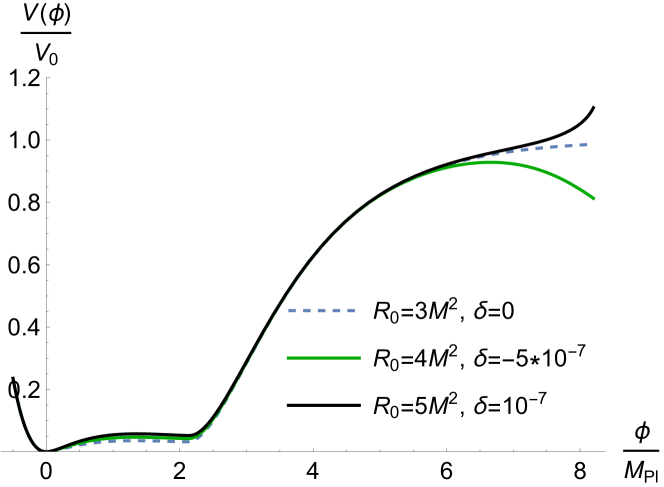
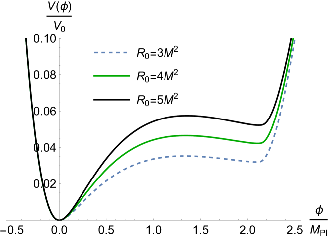
Figure 1: On the left: the inflaton potential having two plateaus for $g=2.25$ and $b=2.89$ with $V_{0}={{3}\over{4}}M^{2}$. On the right: zooming the potential for lower values of $\phi$ with a near-inflection point. The potential is unstable for negative values of $\delta$, and has the infinite plateau for $\delta=0$ describing Starobinsky inflation.

The standard SR conditions are given by $\epsilon_{\rm sr}\ll 1$ and $\left|\eta_{\rm sr}\right|\ll 1$, where

$$\epsilon_{\rm sr}(\phi)={{1}\over{2}}\left({{V^{\prime}(\phi)}\over{V(\phi)}}\right)^{2}\quad{\rm and}\quad\eta_{\rm sr}(\phi)={{V^{\prime\prime}(\phi)}\over{V(\phi)}}~{},$$ (6)

while the time clock is conveniently defined by the number $N$ of e-folds, $N=\int^{t_{end}}_{t_{in}}H(t)dt$, where $H(t)$ is Hubble function. The CMB tilt $n_{s}$ of scalar perturbations and the tensor-to-scalar ratio $r$ are related to the values of the SR parameters at the horizon exit with the standard pivot scale $k_{*}=0.05~{}{\rm Mpc}^{-1}$. In the model [8], the tensor-to-scalar ratio $r$ is well inside the current observational bound, $r<0.032$, and the tilt $n_{s}$ agrees within $1\sigma$ with the current CMB measurements [4, 5, 6], $n_{s}=0.9649\pm 0.0042$, with $\delta\sim 10^{-8}$.

Though an USR phase has dynamics different from SR one, the dimensionless power spectrum of scalar perturbations in the SR-approximation (see Eq. (16) for its definition)

$$P_{\zeta}={{H^{2}}\over{8\pi^{2}\epsilon_{\rm sr}}}$$ (7)

appears to be a good approximation in the USR phase also. The power spectrum in the model [8] in given in Fig. 2. The SR parameter $\epsilon_{\rm sr}$ exponentially drops to very low values during the USR phase.

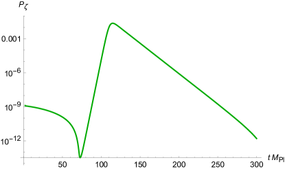
Figure 2: The primordial power spectrum $P_{\zeta}(t)$ of scalar (curvature) perturbations from Eq. (7). A derivation of the spectrum from Mukhanov-Sasaki equation leads to a very close result.

The value of $\eta_{\rm sr}\approx-0.025$ in the USR phase practically does not depend upon the parameters $R_{0}$ and $\delta$. The more illuminating functions are given by the Hubble flow parameters

$$\epsilon_{H}=-{{\dot{H}}\over{H^{2}}}~{},\quad\eta_{H}=\epsilon_{H}-{{\dot{\epsilon}_{H}}\over{2\epsilon_{H}H}}~{}~{}.$$ (8)

Though the $\epsilon_{\rm sr}$ and $\epsilon_{H}$ can be identified, evolution of $\eta_{\rm sr}$ and $\eta_{H}$ is different during the USR phase, see Fig. 3.

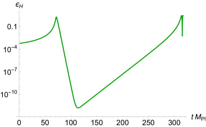
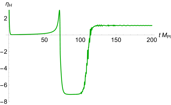
Figure 3: The evolution of $\epsilon_{H}(t)$ and $\eta_{H}(t)$ with the initial conditions $\phi_{in}=7.01$ and $\dot{\phi}_{in}=0$, and the parameters $\delta=2.7\cdot 10^{-8}$ and $R_{0}=3.0~{}M^{2}$. In the USR phase, the value of $\eta_{H}(t)$ is close to $-6$.

The peak in the power spectrum of Fig. 2 is broad and, hence, the peak amplitude of the induced gravitational waves (GW) can be roughly estimated as [22, 23, 24]

$$\Omega_{\mathrm{GW}}\approx 10^{-6}P^{2}_{\zeta}~{}.$$ (9)

The GW frequencies are related to the PBH masses as [25]

$$f_{p}\approx 5.7\left({{M_{\odot}}\over{M_{\mathrm{PBH}}}}\right)^{1/2}10^{-9}~{}\mathrm{Hz}~{},$$ (10)

where $M_{\odot}\approx 2\cdot 10^{33}$ g is the mass of the Sun. In the model under investigation, it leads to the GW frequencies between ${\cal O}(10^{-2})$ Hz and ${\cal O}(10^{-1})$ Hz, which are larger than the GW frequencies between ${\cal O}(10^{-9})$ Hz and ${\cal O}(10^{-7})$ Hz detected by NANOGrav [26].

The PBH-in-DM density fraction $f(k)$ on scale $k$ can be estimated in the Press-Schechter formalism [27] as

$$f(k)={{\Omega_{\rm PBH}(k)}\over{\Omega_{\rm DM}}}\approx{{1.2\cdot 10^{24}\beta_{f}(k)}\over{\sqrt{M_{\rm PBH}(k){\rm g}^{-1}}}}\approx 17.1(k~{}{\rm Mpc})\beta_{f}(k)~{}~{},$$ (11)

where [28, 29]

$$\beta_{f}(k)\simeq{{\sigma(k)}\over{\sqrt{2\pi}\delta_{c}}}e^{-{{\delta^{2}_{c}}\over{2\sigma^{2}(k)}}}~{},\quad\sigma^{2}(k)={{16}\over{81}}\int{{dq}\over{q}}\left({{q}\over{k}}\right)^{4}e^{-q^{2}/k^{2}}P_{\zeta}(q)~{},$$ (12)

with the constant $\delta_{c}$ depending upon the shape of the PBH peak in the power spectrum and representing the density threshold for PBH formation. The integral in Eq. (12) can be estimated as

$$\sigma^{2}\approx{{3.84}\over{81}}P_{\zeta}^{\rm peak}~{},$$ (13)

where $P_{\zeta}^{\rm peak}$ is the value of the power spectrum at the PBH peak. Then Eqs. (11) and (12) imply

$$f(k)\sim{{10^{23}}\over{\sqrt{M_{\rm PBH}(k){\rm g}^{-1}}}}\left({{\sqrt{P_{\zeta}^{\rm peak}}}\over{\delta_{c}}}\right)e^{-9.3\,\delta_{c}^{2}/P_{\zeta}^{\rm peak}}~{}.$$ (14)

This equation demonstrates high sensitivity of the PBH-in-DM fraction upon the value of $\delta^{2}_{c}/P_{\zeta}^{\rm peak}$. In the case of the power spectrum in Fig. 2, we have $\delta_{c}\approx 0.45$ and $P_{\zeta}^{\rm peak}\approx 0.05$. For instance, with the PBH masses between $10^{16}$ g and $10^{20}$ g predicted by our model, eq. (14) gives the PBH fraction in DM between $1\%$ and $100\%$. It is worth mentioning that even a small PBH fraction could have an important role in cosmology [20].

3 Loop corrections

In the $\delta N$ formalism [17] for single-field inflation, a scalar (comoving curvature) perturbation $\delta N\equiv\zeta$ is a function of variation $\delta\phi$ of inflaton $\phi_{i}$ at its initial value,

$$\delta N=N^{\prime}(\phi)\delta\phi+{{N^{\prime\prime}(\phi)}\over{2!}}\delta\phi^{2}+{{N^{\prime\prime\prime}(\phi)}\over{3!}}\delta\phi^{3}+\ldots~{},$$ (15)

where perturbations are not assumed to be small. The power spectrum of scalar perturbations is defined by a two-point function of Fourier components $\zeta_{\bf p}$ as

$$\langle\zeta_{\bf p_{1}}\zeta_{\bf p_{2}}\rangle=(2\pi)^{3}\delta^{3}({\bf{p_{1}}}+{\bf p_{2}})P(p)~{},\quad P_{\zeta}(p)={{k^{3}}\over{2\pi^{2}}}P(p)~{},$$ (16)

where

$$\zeta_{\bf p}=N^{\prime}\delta\phi_{\bf p}+{{N^{\prime\prime}}\over{2!}}\int{{d^{3}q}\over{(2\pi)^{3}}}\delta\phi_{\bf q}\delta\phi_{\bf p-q}+{{N^{\prime\prime\prime}}\over{3!}}\int{{d^{3}q_{1}}\over{(2\pi)^{3}}}{{d^{3}q_{2}}\over{(2\pi)^{3}}}\delta\phi_{\bf q_{1}}\delta\phi_{\bf q_{2}}\delta\phi_{\bf p-q_{1}-q_{2}}+\ldots$$ (17)

in terms of external 3D momenta ${\bf p}$ and loop momenta ${\bf q}$. Substituting Eq. (17) into Eq. (16) yields the loop expansion of the power spectrum $P_{\zeta}(p)$. In order to apply that to a particular model, one has to know the function $N(\phi)$ explicitly. It was derived in Ref. [18],

$$N_{\rm total}(\phi_{i})\simeq{{1}\over{\eta_{\rm sr}}}\ln\Big{[}1+{{\eta_{\rm sr}}\over{\sqrt{2\epsilon_{\rm sr}}}}(\phi_{i}-\phi_{s})\Big{]}-{{1}\over{3}}\ln\Big{[}1+{{3(\phi_{s}-\phi_{e})}\over{\pi_{s}}}\Big{]}+{{1}\over{\eta_{\rm V}}}\ln[-2\eta_{\rm V}\pi_{e}-6\sqrt{2\epsilon_{\rm V}}]~{},$$ (18)

where the first term refers to the SR(I) phase with the initial value $\phi_{i}$ and the end value $\phi_{s}$, the second term refers to the USR phase with the initial momentum value $\pi_{s}$ and the end momentum value $\pi_{e}$, and the third terms refers to the SR(II) phase with the slow-roll parameters $\epsilon_{\rm V}$ and $\eta_{\rm V}$. The subscripts $(s,e)$ refer to values of any quantity at the start and end of the USR phase, respectively. The leading contribution comes from the first term in Eq. (18).

To compute loop corrections, one has to calculate the derivatives $N^{(n)}(\phi)$. The first three derivatives can be estimated as follows:

$$N^{\prime}\approx{{1}\over{\sqrt{2\epsilon_{s}}}}\approx{{e^{-3\Delta N_{\rm USR}}}\over{\sqrt{2\epsilon_{e}}}}~{},\quad N^{\prime\prime}\approx-{{\eta_{\rm sr}}\over{2\epsilon_{s}}}~{},\quad N^{\prime\prime\prime}\approx{{2\eta_{\rm sr}^{2}}\over{(2\epsilon_{s})^{3/2}}}~{}~{},$$ (19)

where $\Delta N_{\rm USR}$ is the duration of the USR phase and $\eta_{\rm sr}\equiv\eta_{\rm sr}(\phi_{s})$.

To compute loop corrections to the amplitude of the power spectrum, we considered the effective action up to the third order with respect to $\delta\phi(\bm{x},t)$ on the background $\phi(t)$,

$$S_{\delta\phi}=S^{(2)}_{\delta\phi}+S^{(3)}_{\delta\phi}=\hbox{\large{${{\textstyle{{1}\over\vphantom{2}\smash{\raise 0.72331pt\hbox{$\scriptstyle{{2}}$}}}}}$}}\int d^{4}x\sqrt{-g}\Big{(}g_{\mu\nu}\partial^{\mu}\delta\phi\partial^{\nu}\delta\phi-V_{,\phi\phi}\delta\phi^{2}\Big{)}+\hbox{\large{${{\textstyle{{1}\over\vphantom{2}\smash{\raise 0.72331pt\hbox{$\scriptstyle{{2}}$}}}}}$}}\int d^{4}x\sqrt{-g}\Big{(}-\hbox{\large{${{\textstyle{{1}\over\vphantom{2}\smash{\raise 0.72331pt\hbox{$\scriptstyle{{3}}$}}}}}$}}V_{,\phi\phi\phi}\delta\phi^{3}\Big{)}.$$ (20)

When using the FLRW background, it reads

$$S_{\delta\phi}=\hbox{\large{${{\textstyle{{1}\over\vphantom{2}\smash{\raise 0.72331pt\hbox{$\scriptstyle{{2}}$}}}}}$}}\int d^{4}x\,a^{3}(t)\Big{[}\dot{\delta\phi}^{2}-a^{-2}(t)(\partial\delta\phi)^{2}-V_{,\phi\phi}\delta\phi^{2}\Big{]}+\int d^{4}x\Big{[}-\hbox{\large{${{\textstyle{{a^{3}(t)}\over\vphantom{2}\smash{\raise 0.72331pt\hbox{$\scriptstyle{{3!}}$}}}}}$}}V_{,\phi\phi\phi}\delta\phi^{3}\Big{]}~{},$$ (21)

where $\partial\equiv\sum_{i}\partial_{i}$ is a sum of spatial derivatives. The standard mode functions arising in the classical equations of motion obtained from a variation of the action (21),

$$u_{k}(\tau)={{H}\over{\sqrt{2k^{3}}}}(1+ik\tau)e^{-ik\tau}~{},$$ (22)

are written down in terms of the conformal time $d\tau=\hbox{\large{${{\textstyle{{dt}\over\vphantom{2}\smash{\raise 0.72331pt\hbox{$\scriptstyle{{a}}$}}}}}$}}$, where $-\infty<\tau\leq 0$. The CMB modes that left the horizon during inflation are given by $u_{k}(0)={{H}\over{\sqrt{2k^{3}}}}$ .

Canonical quantization implies a decomposition into positive and negative parts, as well as the commutation relations (in the interaction picture)

$$\begin{split}&\delta\phi^{I}_{\bf k}(\tau)=\delta\phi^{+}_{\bf k}(\tau)+\delta\phi^{-}_{\bf k}(\tau)=u_{k}(\tau)a_{\bf k}+u_{k}^{*}(\tau)a^{\dagger}_{\bf-k}~{},\\ &[a_{\bf p},a^{\dagger}_{\bf q}]=(2\pi)^{3}\delta^{3}(\bm{p}-\bm{q}),~{}~{}[a_{\bf p},a_{\bf q}]=[a^{\dagger}_{\bf p},a^{\dagger}_{\bf q}]=0~{}.\end{split}$$ (23)

To get the 1-loop correction according to Eqs. (16) and (17), one has to evaluate the three-point correlation function. For this purpose we applied the in-in formalism that gives

$$\langle\delta\phi_{\bf p}\delta\phi_{\bf q}\delta\phi_{\bf-p-q}\rangle=\langle\overline{T}e^{i\int_{t_{0}}^{t}d\widetilde{t}H_{\rm int}}~{}\delta\phi^{I}_{\bf p}\delta\phi^{I}_{\bf q}\delta\phi^{I}_{\bf-p-q}~{}Te^{-i\int_{t_{0}}^{t}d\widetilde{t}H_{\rm int}}\rangle~{},$$ (24)

where $T$ and $\overline{T}$ stand for the time ordering and anti-time ordering respectively, $t_{0}$ and $t$ are the times associated with the subhorizon and superhorizon scales, respectively, and $H_{\rm int}(\tilde{t})$ is the interaction Hamiltonian in the 3rd order,

$$H_{\rm int}(\tilde{t})=\hbox{\large{${{\textstyle{{1}\over\vphantom{2}\smash{\raise 0.72331pt\hbox{$\scriptstyle{{3!}}$}}}}}$}}a^{3}(\tilde{t})V_{,\phi\phi\phi}\int d^{3}x(\delta\phi^{I}(\bm{x},\tilde{t}))^{3}={{1}\over{3!(2\pi)^{6}}}a^{3}(\tilde{t})V_{,\phi\phi\phi}\int d^{3}kd^{3}\lambda\delta\phi^{I}_{\bf k}(\tilde{t})\delta\phi^{I}_{\bm{\lambda}}(\tilde{t})\delta\phi^{I}_{\bf-k-\bm{\lambda}}(\tilde{t})~{}.$$ (25)

The standard (Friedmann and Klein-Gordon) equations of motion yield the following asymptotic approximation for the third derivative of the potential in terms of the Hubble flow parameters (8):

$$V_{,\phi\phi\phi}\simeq-{{3H\dot{\eta_{H}}}\over{2\sqrt{2\epsilon_{H}}}}~{}~{}.$$ (26)

Expanding the T-exponentials in Eq. (24) to the first order with respect to $H_{\rm int}$, we find

$$\begin{split}&\langle\delta\phi_{\bf p}(t)\delta\phi_{\bf q}(t)\delta\phi_{\bf-p-q}(t)\rangle\approx-i\int_{t_{0}}^{t}d\widetilde{t}\langle[\delta\phi^{I}_{\bf p}(t)\delta\phi^{I}_{\bf q}(t)\delta\phi^{I}_{\bf-p-q}(t),H^{int}(\tilde{t})]\rangle\\ &=2{\rm Im}\Bigg{(}\int_{t_{0}}^{t}d\widetilde{t}\langle\delta\phi^{I}_{\bf p}(t)\delta\phi^{I}_{\bf q}(t)\delta\phi^{I}_{\bf-p-q}(t)H^{int}(\tilde{t})\rangle\Bigg{)}~{}.\end{split}$$ (27)

After substituting Eqs. (22), (23), (25) and (26) into Eq. (27) and using Wick’s theorem, we derived the three-point correlator as follows:

$$\begin{split}&\langle\delta\phi_{\bf p}\delta\phi_{\bf q}\delta\phi_{\bf-p-q}\rangle=\\ &=-{{1}\over{2(2\pi)^{6}}}{\rm Im}\Bigg{(}\int_{-\infty}^{0}d\widetilde{\tau}a^{3}(\tilde{\tau}){{H\eta^{\prime}(\widetilde{\tau})}\over{\sqrt{2\epsilon}}}\int d^{3}kd^{3}\lambda\langle\delta\phi^{+}_{\bf p}\delta\phi^{+}_{\bf q}\delta\phi^{+}_{\bf-p-q}\delta\phi^{-}_{\bf k}(\tilde{\tau})\delta\phi^{-}_{\bm{\lambda}}(\tilde{\tau})\delta\phi^{-}_{\bf-k-\bm{\lambda}}(\tilde{\tau})\rangle\Bigg{)}\\ &=-{{\Delta\eta}\over{2(2\pi)^{6}}}{\rm Im}\Bigg{(}{{H_{e}a_{e}^{3}}\over{\sqrt{2\epsilon_{e}}}}\int d^{3}kd^{3}\lambda\langle\delta\phi^{+}_{\bf p}(\tau)\delta\phi^{+}_{\bf q}(\tau)\delta\phi^{+}_{\bf-p-q}(\tau)\delta\phi^{-}_{\bf k}(\tau_{e})\delta\phi^{-}_{\bm{\lambda}}(\tau_{e})\delta\phi^{-}_{\bf-k-\bm{\lambda}}(\tau_{e})\rangle\Bigg{)}\\ &\approx{{3!(2\pi)^{3}\left|\Delta\eta\right|}\over{2}}{\rm Im}\Bigg{(}{{H^{4}_{e}a_{e}^{3}}\over{\sqrt{2\epsilon_{e}}}}{{H^{3}_{0}(1-iq\tau_{e})^{2}}\over{(2q^{3})^{2}2p^{3}}}e^{2iq\tau_{e}}\Bigg{)}~{},\end{split}$$ (28)

where the $H(0)=H_{0}$ denoted the Hubble value during the SR(I), the reference time was chosen at $\tau=0$ because we were only interested in the power spectrum on super-horizon scales relevant to CMB, and $p\ll q$. To avoid divergences, the vacuum expectation value was normalized by the volume of the entire system.

Dynamics of the parameter $\eta_{H}$ implies it is essentially constant everywhere except for the moments of a decrease or an increase (corresponding to $\tau_{s}$ and $\tau_{e}$, respectively), while the moment of the increase is particularly significant (see Fig. 3). The approximate solution (18) to the equations of motion in our model is smooth as well as the corresponding $\eta_{H}(t)$ function defined by the second equation (8). However, to simplify loop calculations, we found useful to employ the derivative of $\eta_{H}$ with respect to the conformal time as the (Dirac) delta function, $\eta_{H}^{\prime}(\tau)\sim\delta(\tau-\tau_{e})\Delta\eta$, where $\Delta\eta\approx-6$ is the depth of the pit, inside integrations, which corresponds to a sharp transition. Via integration, the delta function fixes the entire integrand at the time $\tau_{e}$ corresponding to the end of the USR stage.

Equations (15), (16) and (17) lead to a recovery of the tree-level contribution (7) as the leading term in the loop expansion of the power spectrum, as well as the first (1-loop) contribution as follows:

$$P^{\rm 1-loop}_{\zeta}(p)\equiv{{N^{\prime}N^{\prime\prime}}\over{2}}\int{{d^{3}q}\over{(2\pi)^{3}}}\langle\delta\phi_{\bf p}\delta\phi_{\bf q}\delta\phi_{\bf-p-q}\rangle~{}.$$ (29)

After substituting Eqs. (19) and (28) into Eq. (29) we found

$$\begin{split}&P^{\rm 1-loop}_{\zeta}(p)\approx{{\eta_{\rm sr}e^{-3\Delta N_{\rm USR}}}\over{2\sqrt{2\epsilon_{e}}2\epsilon_{s}}}\int_{\rm USR}dq(4\pi q^{2}){{3!\left|\Delta\eta\right|}\over{2}}{\rm Im}\Bigg{(}{{H^{4}_{e}a_{e}^{3}}\over{\sqrt{2\epsilon_{e}}}}{{H^{3}_{0}(1-iq\tau_{e})^{2}}\over{(2q^{3})^{2}2p^{3}}}e^{2iq\tau_{e}}\Bigg{)}\\ &\approx\eta_{\rm sr}e^{-3\Delta N_{\rm USR}}P_{\zeta}(p)P^{\rm PBH}_{\zeta}{{(2\pi)^{3}\left|\Delta\eta\right|}\over{4}}\Bigg{(}{{H_{0}}\over{H_{e}}}\Bigg{)}~{},\end{split}$$ (30)

where $P^{\rm PBH}_{\zeta}\sim 10^{-2}$ is the amplitude of the power spectrum on the small scales associated with the short-wavelength PBH modes exiting the horizon during the USR phase of inflation. The value of $H_{0}/H_{e}\approx 5$ defines the ratio of the inflation and PBH scales in our model.

It is evident from Eq. (30) that the dependence of the 1-loop correction upon the slow-roll parameter $\eta_{sr}$ comes from the second derivative $N^{\prime\prime}$, the exponential factor depending upon $\Delta N_{\rm USR}$ arises from the first derivative $N^{\prime}$, and the dependence upon ${P}^{\rm PBH}_{\zeta}$ and $\Delta\eta$ comes from the third derivative $V_{,\phi\phi\phi}$, namely, from the $\eta^{\prime}(\tau)$.

A detailed calculation of the higher-loop corrections is very involved and will not be given here. However, it is possible to get a rough estimate of the 2-loop correction by using the approximative formula given in Ref. [18],

$$P^{\rm 2-loop}_{\zeta}(p)\approx{{N^{\prime}N^{\prime\prime\prime}}\over{3!}}|\delta\phi_{\bf p}|^{2}\int{{d^{3}q}\over{(2\pi)^{3}}}|\delta\phi_{\bf q}|^{2}\sim\eta^{2}_{\rm sr}\Delta N_{\rm USR}P_{\zeta}(p)P^{\rm PBH}_{\zeta}~{}.$$ (31)

In our model, according to the plot on the right-hand-side of Fig. 3, we have $\Delta N_{\rm USR}\approx 3.1$.

Therefore, the relative size of the 1-loop and 2-loop corrections from PBH production to the power spectrum at the CMB pivot scale $k^{*}=0.05$ are

$${{P_{\zeta}^{\rm 1-loop}(k^{*}=0.05)}\over{P_{\zeta}(k^{*}=0.05)}}\approx\eta_{\rm sr}e^{-3\Delta N_{\rm USR}}P^{\rm PBH}_{\zeta}{{(2\pi)^{3}\left|\Delta\eta\right|}\over{4}}\Bigg{(}{{H_{0}}\over{H_{e}}}\Bigg{)}\approx 10^{-4}$$ (32)

and

$${{P_{\zeta}^{\rm 2-loop}(k^{*}=0.05)}\over{P_{\zeta}(k^{*}=0.05)}}\sim\eta^{2}_{\rm sr}\Delta N_{\rm USR}P^{\rm PBH}_{\zeta}\approx 10^{-5}~{},$$ (33)

where we have used $P_{\zeta}(k^{*}=0.05)\approx 2\cdot 10^{-9}$ for the CMB power spectrum. Therefore, the one-loop contribution is suppressed by the factor $\eta_{\rm sr}e^{-3\Delta N_{\rm USR}}$, whereas the two-loop contribution is suppressed by $\eta^{2}_{\rm sr}\Delta N_{\rm USR}$ (we recall that $\eta_{\rm sr}\approx-0.025$ in our model). Therefore, the longer the duration of the USR phase, the (exponentially) less significant the one-loop correction becomes. As regards the higher $n$-loop corrections, their structure includes the suppression factor $\eta^{n}_{\rm sr}P^{\rm PBH}_{\zeta}\sim 10^{-2n-2}$ so that they are expected to be negligible too.

The basic reasons for the smallness of loop corrections in our model are due to (i) smooth transitions between the SR and USR phases, in agreement with Ref. [18], and (ii) the duration of the USR phase $\Delta N_{\rm USR}>1$.

The sharpness of the SR-to-USR-to-SR transitions can be quantitatively estimated by the parameter $h$ defined by [16]

$$h=-6{{\sqrt{2\epsilon_{\rm V}}}\over{\pi_{e}}}\approx-6\sqrt{{{\epsilon_{\rm V}}\over{\epsilon_{s}}}}e^{-3\Delta N_{\rm USR}}~{},$$ (34)

where $\pi_{e}$ is the inflaton momentum at the end of the USR inflation, $\epsilon_{s}$ and $\epsilon_{\rm V}$ are the values of the SR parameter at the end of the USR phase and at the beginning of the SRII phase, respectively. In our model, we have the small value of $h\sim 10^{-3}$, which implies the smooth transitions.

4 Conclusion

It follows from our results in Sec. 3 that the modified gravity model [8] of Starobinsky inflation with PBH production is not ruled out by quantum loop corrections because the latter are relatively small by the factor of $10^{-4}$ against the tree-level (classical) contribution. The key role in this conclusion was played by the derivatives of the function $N(\phi)$ during the USR phase and the prolonged duration $\Delta N_{\rm USR}$, which led to the suppression of loop contributions.

References

• [1] A. A. Starobinsky, “A new type of isotropic cosmological models without singularity,” Phys. Lett. B 91 no. 1, (1980) 99 – 102.
• [2] S. V. Ketov, “On the equivalence of Starobinsky and Higgs inflationary models in gravity and supergravity,” J. Phys. A 53 no. 8, (2020) 084001, arXiv:1911.01008 [hep-th].
• [3] V. R. Ivanov, S. V. Ketov, E. O. Pozdeeva, and S. Y. Vernov, “Analytic extensions of Starobinsky model of inflation,” JCAP 03 no. 03, (2022) 058, arXiv:2111.09058 [gr-qc].
• [4] Planck Collaboration, Y. Akrami et al., “Planck 2018 results. X. Constraints on inflation,” Astron. Astrophys. 641 (2020) A10, arXiv:1807.06211 [astro-ph.CO].
• [5] BICEP, Keck Collaboration, P. A. R. Ade et al., “Improved Constraints on Primordial Gravitational Waves using Planck, WMAP, and BICEP/Keck Observations through the 2018 Observing Season,” Phys. Rev. Lett. 127 no. 15, (2021) 151301, arXiv:2110.00483 [astro-ph.CO].
• [6] M. Tristram et al., “Improved limits on the tensor-to-scalar ratio using BICEP and Planck data,” Phys. Rev. D 105 no. 8, (2022) 083524, arXiv:2112.07961 [astro-ph.CO].
• [7] D. Frolovsky, S. V. Ketov, and S. Saburov, “Formation of primordial black holes after Starobinsky inflation,” Mod. Phys. Lett. A 37 no. 21, (2022) 2250135, arXiv:2205.00603 [astro-ph.CO].
• [8] S. Saburov and S. V. Ketov, “Improved Model of Primordial Black Hole Formation after Starobinsky Inflation,” Universe 9 no. 7, (2023) 323, arXiv:2306.06597 [gr-qc].
• [9] S. R. Geller, W. Qin, E. McDonough, and D. I. Kaiser, “Primordial black holes from multifield inflation with nonminimal couplings,” Phys. Rev. D 106 no. 6, (2022) 063535, arXiv:2205.04471 [hep-th].
• [10] P. S. Cole, A. D. Gow, C. T. Byrnes, and S. P. Patil, “Primordial black holes from single-field inflation: a fine-tuning audit,” arXiv:2304.01997 [astro-ph.CO].
• [11] A. Karam, N. Koivunen, E. Tomberg, V. Vaskonen, and H. Veermäe, “Anatomy of single-field inflationary models for primordial black holes,” JCAP 03 (2023) 013, arXiv:2205.13540 [astro-ph.CO].
• [12] J. Kristiano and J. Yokoyama, “Ruling Out Primordial Black Hole Formation From Single-Field Inflation,” arXiv:2211.03395 [hep-th].
• [13] S. Choudhury, S. Panda, and M. Sami, “Quantum loop effects on the power spectrum and constraints on primordial black holes,” JCAP 11 (2023) 066, arXiv:2303.06066 [astro-ph.CO].
• [14] S.-L. Cheng, D.-S. Lee, and K.-W. Ng, “Primordial perturbations from ultra-slow-roll single-field inflation with quantum loop effects,” arXiv:2305.16810 [astro-ph.CO].
• [15] M. W. Davies, L. Iacconi, and D. J. Mulryne, “Numerical 1-loop correction from a potential yielding ultra-slow-roll dynamics,” arXiv:2312.05694 [astro-ph.CO].
• [16] Y.-F. Cai, X. Chen, M. H. Namjoo, M. Sasaki, D.-G. Wang, and Z. Wang, “Revisiting non-Gaussianity from non-attractor inflation models,” JCAP 05 (2018) 012, arXiv:1712.09998 [astro-ph.CO].
• [17] A. A. Abolhasani, H. Firouzjahi, A. Naruko, and M. Sasaki, Delta N Formalism in Cosmological Perturbation Theory. WSP, 2, 2019.
• [18] H. Firouzjahi and A. Riotto, “Primordial Black Holes and Loops in Single-Field Inflation,” arXiv:2304.07801 [astro-ph.CO].
• [19] S. A. Appleby, R. A. Battye, and A. A. Starobinsky, “Curing singularities in cosmological evolution of F(R) gravity,” JCAP 06 (2010) 005, arXiv:0909.1737 [astro-ph.CO].
• [20] B. Carr, K. Kohri, Y. Sendouda, and J. Yokoyama, “Constraints on primordial black holes,” Rept. Prog. Phys. 84 no. 11, (2021) 116902, arXiv:2002.12778 [astro-ph.CO].
• [21] K.-i. Maeda, “Towards the Einstein-Hilbert Action via Conformal Transformation,” Phys. Rev. D 39 (1989) 3159.
• [22] S. Pi and M. Sasaki, “Gravitational Waves Induced by Scalar Perturbations with a Lognormal Peak,” JCAP 09 (2020) 037, arXiv:2005.12306 [gr-qc].
• [23] G. Domènech, “Scalar Induced Gravitational Waves Review,” Universe 7 no. 11, (2021) 398, arXiv:2109.01398 [gr-qc].
• [24] D. Frolovsky and S. V. Ketov, “Fitting power spectrum of scalar perturbations for primordial black hole production during inflation,” Astronomy 2 (2023) 47–57, arXiv:2302.06153 [astro-ph.CO].
• [25] V. De Luca, G. Franciolini, and A. Riotto, “NANOGrav Data Hints at Primordial Black Holes as Dark Matter,” Phys. Rev. Lett. 126 no. 4, (2021) 041303, arXiv:2009.08268 [astro-ph.CO].
• [26] NANOGrav Collaboration, G. Agazie et al., “The NANOGrav 15 yr Data Set: Evidence for a Gravitational-wave Background,” Astrophys. J. Lett. 951 no. 1, (2023) L8, arXiv:2306.16213 [astro-ph.HE].
• [27] W. H. Press and P. Schechter, “Formation of galaxies and clusters of galaxies by selfsimilar gravitational condensation,” Astrophys. J. 187 (1974) 425–438.
• [28] K. Inomata, M. Kawasaki, K. Mukaida, Y. Tada, and T. T. Yanagida, “Inflationary Primordial Black Holes as All Dark Matter,” Phys. Rev. D 96 no. 4, (2017) 043504, arXiv:1701.02544 [astro-ph.CO].
• [29] Y. Aldabergenov, A. Addazi, and S. V. Ketov, “Primordial black holes from modified supergravity,” Eur. Phys. J. C 80 no. 10, (2020) 917, arXiv:2006.16641 [hep-th].