InterpretCC: Conditional Computation for Inherently Interpretable Neural Networks

Abstract

Real-world interpretability for neural networks is a tradeoff between three concerns: 1) it requires humans to trust the explanation approximation (e.g. post-hoc approaches), 2) it compromises the understandability of the explanation (e.g. automatically identified feature masks), and 3) it compromises the model performance (e.g. decision trees). These shortcomings are unacceptable for human-facing domains, like education, healthcare, or natural language, which require trustworthy explanations, actionable interpretations, and accurate predictions. In this work, we present InterpretCC (interpretable conditional computation), a family of interpretable-by-design neural networks that guarantee human-centric interpretability while maintaining comparable performance to state-of-the-art models by adaptively and sparsely activating features before prediction. We extend this idea into an interpretable mixture-of-experts model, that allows humans to specify topics of interest, discretely separates the feature space for each data point into topical subnetworks, and adaptively and sparsely activates these topical subnetworks. We demonstrate variations of the InterpretCC architecture for text and tabular data across several real-world benchmarks: six online education courses, news classification, breast cancer diagnosis, and review sentiment.

1 Introduction

In recent years, the steep rise in popularity of neural networks has come with a severe weakness: the lack of interpretability of their predictions. Neural networks are considered as black-box models due to their high number of parameters and complex operations. Therefore, humans cannot yet understand how the features impact the network decisions under the hood.

Interpretable models and techniques are a relatively new field of research in the machine-learning community. As a result of increasing interest in providing explanations for black-box models, several popular methods have been proposed. These include local instance-based approaches, such as LIME (Ribeiro et al., 2016) and SHAP (Lundberg & Lee, 2017), as well as using adversarial examples for counterfactual explanations (Dhurandhar et al., 2018). Gradient methods such as Grad-CAM (Selvaraju et al., 2019) assess the contribution of a model component to the output of the model have proven effective, along with concept-based explanations such as TCAV (Kim et al., 2017) and DTCAV (Ghorbani et al., 2019).

Most explainability methods for black-box models (i.e. neural networks) are post hoc, applied after model training. These require the user to trust the explainer’s approximation of the true explanation, which has been shown to be systematically biased and inconsistent (Krishna et al., 2022; Swamy et al., 2022c). On the other hand, intrinsically interpretable models (Chen et al., 2019; Sawada & Nakamura, 2022; Nauta et al., 2023) have mainly focused on example-based approaches, overwhelmingly in the image domain and rarely in time-series, tabular, or text modalities. Very recent interpretable-by-design literature in mixture-of-experts models has highlighted a hierarchical neural network structure with subnetworks, combining interpretable experts (i.e. decision trees) with DNNs for partially interpretable points (Ismail et al., 2023), selectively activating experts (Li et al., 2022), or extracting automatic concept for routing (You et al., 2023). However, none of these architectures put the human decision-making process at the center of the design, refusing to compromise on interpretability. The goal of this paper is to propose a interpretable-by-design neural network architecture that achieves guaranteed interpretability (certainty), and human-centric explanations (understandability) while maintaining comparable predictive performance. To achieve this, we consider using conditional computation in neural networks to craft interpretable neural pathways.

We aim to answer the question: Can we learn meaningful computation paths that give human-focused insight into the model decisions? Our model’s reasoning enables a statement of the form: ”This entry was predicted to be X because and only because it was assigned to human-interpretable categories A and B”. We refer to interpretability from the users’ perspective, focusing on the model’s local reasoning for a decision on a specific data point, as opposed to a global understanding of the model’s internals.

We provide the following contributions with our family of InterpretCC models:

• An architecture for a simple, interpretable-by-design neural network using instance-dependent gating.

• An architecture for an interpretable mixture-of-experts model that leverages human-specified group routing to distinctly separate the feature space and sparsely activate specific experts.

• Evaluation on real-world, human-centric modalities that are not often covered by interpretable-by-design deep learning approaches: time-series (education), tabular (healthcare), and text datasets (sentiment, news).

Our models are characterized by sparse explicit routing, truncated feature spaces, and adaptivity per data point. These traits are extremely important for human-centric trustworthiness as it provides clarity, consiseness, and personalization in explanations (Miller, 2019; Swamy et al., 2023b). We provide our code and experiments open source.

2 Methodology

2.1 Problem Formulation

Given an input $x$, the objective of our approach is to select a sparse subset $x$ that will be used to compute the output. In this work, we propose two architectures:

Feature Gating: The approach selects a subset of the features by applying a sparse mask $\mathcal{M}(x)$ on the input before processing it by a model $f$. The output is given by:

$$f(\mathcal{M}(x)\odot x)$$ (1)

where $\odot$ is the Hadamard product.

Gated Routing: A sparse mixture of models (Fedus et al., 2022a) applied on human-interpretable groups of features where each expert is assigned to a group of features:

$$\sum_{i=1}^{K}G(x)_{i}\cdot f_{i}(\mathcal{M}_{\mathcal{G}}(x)_{i}\odot x)$$ (2)

where $\mathcal{M}_{\mathcal{G}}(x)_{i}$ is a binary mask that selects only the features belonging to the $i$-th group, $f_{i}$ is the expert model associated with the $i$-th group, and $G(x)_{i}$ is the output of the gating network for group $i$. In Sections 2.2 and 2.3, we give an in-depth description of both our approaches.

In our experiments, we are considering 3 types of inputs:

• Tabular features: the input is a vector of dimension $n$: $x\in\mathds{R}^{n}$. In that case, the mask in the Feature Gating is a sparse vector $\mathcal{M}(x)\in[0,1]^{n}$ indicating which tabular feature to use and how important they are (if the weight is non 0) and the groups consist of subsets of the set of features.

• Text: the input is a sequence of $n$ tokens: $x=[t_{1},t_{2},\cdots,x_{t}]$. In that case, the mask in the Feature Gating is a sparse binary vector $\mathcal{M}(x)\in\{0,1\}^{n}$ that indicates which token to use and each group consists of a subset of the tokens.

• Time Series: the input is a time series of $n$ features across $T$ timesteps: $x\in\mathds{R}^{n\times T}$. In that case, the same mask in the Feature Gating model is applied at each timestep and indicates which feature to use. The groups are composed of distinct time series, each consisting of a subset of the attributes. Therefore, each expert processes a complete time series composed of features belonging to the same group.

Conditional Computation. InterpretCC is inspired by the idea of conditional computation, which selectively activates parts of a neural network at a time. Conditional computation was introduced to address the expensive training and evaluation time costs of neural networks (Bengio et al., 2013; Davis & Arel, 2013). Bengio et al. outline how block dropout conditional computation policies can be optimized using reinforcement learning (2015). Verelst et al. applied the conditional computation method to human pose estimation, an inherently spatially sparse task, to increase processing speed (2019). To achieve this, a residual block was introduced in which a small gating branch learns which spatial positions should be evaluated. These discrete gating decisions are trained end-to-end using Gumbel-Softmax, in combination with a sparsity criterion. With the InterpretCC models, we extend a similar routing idea with instance-dependent gating decisions (Jiang et al., 2024; Fedus et al., 2022b), for an interpretability objective as opposed to an efficiency or performance objective.

2.2 Feature Gating

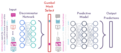
Figure 1: Feature Gating architecture - (i) features passed as input to a discriminator network which outputs a feature activation mask; (ii) features passed individually as input to sub-network + sigmoid for prediction; (iii) activated features’ corresponding predictions averaged for final output.

The Feature Gating architecture illustrated in Figure 1 serves as the first step towards using conditional computation paths for interpretability. The features are first passed through a discriminator network $D$ whose purpose is to select which features to use for computing the output. The discriminator network’s output $D(x)$ must have the same dimension as the input so that each dimension of the output is associated with a feature. The Gumbel-SoftMax trick (Jang et al., 2017) is then applied on each dimension of $D(x)$ to select which features to use in a differentiable way. Each feature $j$ is considered activated (the associated value in the mask is non-zero) if the output of the Gumbel-SoftMax is greater than a threshold $\tau$ whose value is a hyperparameter. The Gumbel-SoftMax enables our model to adaptively select the number of activated features according to each instance. This means that for instances that are straightforward to classify, the Feature Gating architecture might only use two features, whereas for instances that are more complex to classify, it could decide to utilize more features. A further discussion of the Gumbel-Softmax and its implementation in our architecture is detailed in Appendix C. In summary, the mask $\mathcal{M}(x)$ is computed using a discriminator network, followed by the Gumbel-SoftMax trick on each feature along with a threshold $\tau$. As described in equation 1, once the mask is computed, we use it to remove features from the input $x$. The output is computed using a model $f$ on the masked input, and since the explainability is at the feature level, using a ”black box” model for $f$ does not detract from the interpretability.

2.3 Group Routing

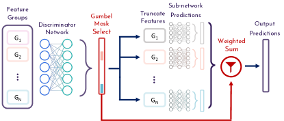
Figure 2: Group Routing architecture: (i) features passed through discriminator network which outputs a route activation mask (ii) features split by group to be passed as input to corresponding expert sub-network for prediction (iii) activated routes’ predictions are aggregated through a weighted sum for final output.

Our follow-up approach Group Routing builds upon the instance-dependent gating architecture. As displayed in Figure 2 instead of selecting features individually, the mask is applied to human interpretable groups of features. Doing so encourages cross-feature interactions while maintaining a meaningful grouping for human users and practitioners. To select the features belonging to group $i$, we use a binary mask $\mathcal{M}_{\mathcal{G}}(x)_{i}$ that is computed using human-specified rules. In section 3, we give an in-depth description of our approach to compute $\mathcal{M}_{\mathcal{G}}(x)_{i}$ for each dataset used in our experiments. Group Routing is a sparse mixture of models utilizing a gating network to assign a weight $G(x)_{i}$ to each group. This process mirrors that of Feature Gating, starting with a discriminator network $D_{\mathcal{G}}$ whose output has $K$ dimensions ($K$ begin the number of groups). It then applies the Gumbel-SoftMax and a threshold $\tau_{\mathcal{G}}$ to each group. As indicated in equation 2, the output of the model is a weighted sum of the output of each expert $f_{i}$ that only uses the features from the $i$-th group as input. Using our sparsity criteria, we ensure that few groups are used to compute the output, making the Group Routing inherently interpretable at the group level, regardless of the types of models used as experts. Group Routing also exhibits several traits in efficient inference without compromising the number of parameters the model can use at training. During the training phase, we employ soft masking, allowing all weights $G(x)_{i}$ to remain non-zero, thus granting the model access to every expert. This approach allows the model to leverage the full set of parameters during training, enhancing the training efficiency. However, at inference time, we switch to using a hard mask, making the weights sparse. This method allows for interpretability and efficiency at inference.

3 Prediction Setting

We apply the InterpretCC framework to three contexts: education, news/sentiment classification, and healthcare, covering different input types: time series, text, and tabular.

3.1 Education

In the education (EDU) context, we predict student success early in massive open online courses (MOOCs).

Data Set: This setting comprises student clickstream data from six different MOOCs. The raw clickstream input is transformed into weekly time-series features that have proven useful for student success prediction in previous literature (e.g. total video clicks, forum interactions). We incorporate weekly features from multiple papers (Lallé & Conati, 2020; Boroujeni et al., 2016; Chen & Cui, 2020; Marras et al., 2021), resulting in 45 input features. We refer to this approach as routing by paper. Since we are interested in early prediction, we only use the first $40\%$ of time steps as input to our models. We pad the features such that each sample has the same number of time steps.

Grouping: To derive human-interpretable concepts from the dataset, we turn to learning science literature. In routing by paper, we create 10 distinct feature subsets based on handcrafted initial input features from 10 papers, directing each to a specific expert subnetwork. For routing by pattern, we organize features according to six learning dimensions identified by (Asadi et al., 2022) and detailed in Table 1—effort, consistency, regularity, proactivity, control, and assessment—based on (Mejia et al., 2022), with a focus on these dimensions in an extended experiment. Thirdly, routing by Large Language Model (LLM), uses GPT-4’s capabilities, to aid humans in feature grouping (Achiam et al., 2023). GPT-4 is prompted as an ’expert learning scientist’ to group the features into self-regulated behavior categories that are easy to understand, which are then used to separate the features for InterpretCC. More details are included in Appendix A.

Dimensions	Corresponding measures	Student patterns
Effort	Total time online Total video clicks	Higher intensity Lower intensity
Consistency	Mean session duration Relative time online Relative video clicks	Uniform First half Second half
Regularity	Periodicity of week day Periodicity of week hour Periodicity of day hour	Higher peaks Lower peaks
Proactivity	Content anticipation Delay in lecture view	Anticipated Delayed
Control	Fraction time spent (video) Pause action frequency Average change rate	Higher intensity Lower intensity
Assessment	Competency strength Student shape	Higher intensity Lower intensity

Table 1: Routing by pattern uses learning dimensions from (Mejia et al., 2022) to create interpretable feature groupings.

3.2 Text Classification

In the news categorization setting (AG News), we predict a news category given a title and description of a real-world article. In the sentiment prediction setting (SST), we predict a binary sentiment from a sentence fragment sourced from a movie review.

Data Sets: AG News Corpus (AG-NEWS) is a collection of news articles from four news categories: ‘World‘, ‘Sports‘, ‘Business‘, ‘Sci/Tech‘ (Zhang et al., 2015). We use 36,000 samples and 3,000 test samples that are evenly distributed across categories. The Stanford Sentiment Treebank (SST) is a text dataset that is a well-known sentiment classification benchmark as an extension of the Movie Review Database (MRD) (Socher et al., 2013). SST comprises 11,855 individual sentences taken from movie reviews, each labeled by three annotators. It includes two sets of labels: one for binary sentiment classification and one for multiclass. We use it for binary classification to show a different setting than the multiclass classification in AG-News.

Grouping: The InterpretCC routing model requires an assignment of words to subnetworks. For this, we use the Dewey Decimal Code (DDC) for librarians and its hierarchy of topics for book classification to create 10 subnetworks, as showcased by topic in Table 2 (Satija, 2013). Each word is assigned to a subcategory (i.e. the word ‘school‘ is assigned to the subcategory ‘education‘ under category 300 for ‘social sciences‘) and routed to the appropriate parent network. The decision to use the DDC was to use subnetworks that were standardized, pervasive in daily life and clearly human-understandable. To conduct this assignment, we utilize SentenceBERT from the sentence-transformers library to encode the subtopics for each DDC heading (i.e. all of 010, 020, 030, etc. for the category 000) (Reimers & Gurevych, 2019). We also use SentenceBERT to encode each word, then assign each word to the most similar DDC category in embedding space with cosine similarity. The reasoning for the use SentenceBERT is to capture the broader context of multi-word category headings.

Code	Field of Study
000	Computer Science, Information
	and General Works
100	Philosophy and Psychology
200	Religion
300	Social Sciences
400	Language
500	Pure science
600	Technology
700	Arts and recreation
800	Literature
900	History and geography

Table 2: Dewey Decimal Classification (Scott & SCOTT, 1998). Each code represents a subnetwork in the text variations of the InterpretCC framework.

3.3 Healthcare

In the health setting (Breast Cancer), we conduct a diagnosis prediction for whether a tissue is malignant (1) or benign (0) based on descriptive features of three cells.

Data Set: The Wisconsin Breast Cancer dataset (Breast Cancer) is a tabular dataset attempting to identify the presence of cancerous tissue from an image of a fine needle aspirate (FNA) of a breast mass (Wolberg et al., 1995). It contains 30 features (10 from each of 3 cell nuclei) along with Malignant (1) or Benign (0) diagnoses for 569 patients.

Grouping: For the grouping logic, we simply group each cell nuclei and relevant features in a separate subnetwork.

4 Experimental Results

Through the following experiments, we will show the performance of the feature gating model against baselines, the performance of the group routing models against baselines, and a deeper analysis in to the practical interpretability of each approach. Our experiments will cover four datasets, and show that in each dataset the performance of InterpretCC is comparable to that of other models.
Experimental Setup: Many MOOC courses have a low passing rate (below 30%), and thus the data set has a heavy class imbalance. Therefore, for the EDU datasets, we use balanced accuracy for evaluation. We perform an 80-10-10 train-validation-test data split that is stratified on the output label in order to properly conserve the class imbalance in each subset to accurately perform our analysis. On the other datasets (text, tabular), the class split is more balanced, so we use accuracy as our evaluation metric. We experiment with the sparsity criterion for feature gating across the 6 online education courses, comparing feature gating with L1 regularization and Annealing L1 regularization in comparison to the baseline BiLSTM model, as discussed in App. B. We note that L1 regularization is substantially more stable than Annealing, and therefore use L1 regularization throughout the following experiments.

4.1 Base Prediction Module

For the education task, previous literature has relied on using BiLSTMs for best predictive performance (Swamy et al., 2022c; Marras et al., 2021). Thus, for comparative benchmarking, the most performant BiLSTM setting reported by Swamy et al. is used as a baseline model (2022b). For the AG News task, we use a fine-tuned DistilBERT as a baseline, and for the SST task, we use a different, finetuned DistilBERT. These choices were made as the baselines have also been reported in related literature (Yang et al., 2019; HF Canonical Model Maintainers, 2022). For the group routing experiments, we compare with a top-k expert network solution with k=2 for global routing. This is similar to the mixture-of-expert approaches presented by Jiang et al. and Li et al., except that their models make a choice of experts in each layer, which significantly reduces interpretability, while we make one global expert choice (2024; 2022). The results of the baseline are presented in comparison to feature gating approaches in Table 3.

4.2 Feature Gating

Performance: Table 3 shows the performance in terms of balanced accuracy (including means and $99\%$ confidence intervals) of our feature gating approach on the EDU, AG News, SST, and Breast Cancer data sets. For the EDU data sets, we observe that InterpretCC improves performance with respect to the baseline for two courses (DSP, HWTS) and shows comparable performance for the four other courses (indicated by the overlapping confidence intervals). Also for the text-based data sets AG News and SST, performance between our interpretable architecture and the baseline is comparable. For only the Breast Cancer dataset, feature gating decreases predictive performance, indicating that for this dataset, a higher number of the available features is necessary for prediction.

	Dataset	Baseline	InterpretCC Feature Gating
EDU	DSP	82.43 +/- 2.24	90.75 +/- 0.01
	Geo	71.81 +/- 4.25	71.92 +/- 0.01
	HWTS	73.53 +/- 5.01	82.89 +/- 0.04
	Structure	52.95 +/- 2.04	50.00 +/- 0.01
	Ventures	51.04 +/- 5.52	52.83 +/- 0.03
	VA	76.58 +/- 2.52	77.80 +/- 0.01
Text	AG-News	89.93 +/- 3.32	85.72 +/- 5.31
	SST	91.12 +/- 2.03	88.21 +/- 3.41
Health	Breast Cancer	89.70 +/- 1.05	74.67 +/- 9.52

Table 3: InterpretCC Feature Gating Performance: Performance in terms of balanced accuracy (averages and $99\%$ confidence intervals) on EDU, Text, and Health datasets in comparison to baselines.

Sparsity: Figure 3 illustrates the percentage of activated features per data point. We observe that for the EDU data sets, only a fraction of the features (VA: $11.8\%$, Geo: $9.5\%$) are activated per data point and the standard deviation is low. Indeed, for VA, only $8$ out of $45$ features are activated at least once, while for $Geo$ only $9$ out of $45$ features are activated at least once. For Breast Cancer data set, more features seem to be needed to make the prediction: about $x\%$ of the features are activated per data point. For the text-based data set, the number of available features (words) varies per data point. The AG News consists of news articles (average number of words per article: $35$) and again, only a small percentage of words is activated for each article. The SST data set contains sentences of variable length, with the shortest one containing only $1$ word (average number of words per sentence: $7$). This variability explains the higher percentage of features selected per data point ($59.8\%$) as well as the high standard deviation.

The achieved sparsity, concisely indicating the most important features in the original data set (especially for EDU and AG News, constitutes a major advantage of our feature gating approach. In comparison, popular post-hoc explainers tend to select a wider range of features as important (e.g., in previous work (Swamy et al., 2022c) on the EDU datasets, LIME and SHAP (Ribeiro et al., 2016; Lundberg & Lee, 2017) indicated broad importance over input features).

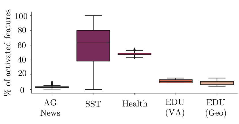
Figure 3: InterpretCC Feature Gating Sparsity: Percentage of features activated per data point across five representative datasets.

InterpretCC feature gating has the significant advantage of providing a simple, sparse feature selection without compromising performance.

4.3 Group Routing

In the following experiments, we examine the InterpretCC group routing architecture across four datasets, in comparison with a global top-k baseline.

Performance: As shown in Table 4, InterpretCC Routing has the potential to improve upon baseline performance, depending on the selected grouping. We for example achieve a $10\%$ increase in performance when grouping using patterns or GPT-4 for the Geo course. For the other courses, performance of our approach is similar to baseline performance. Only for VA, group routing leads to a decrease in balanced accuracy. Note that Structure and Ventures are courses with a small population as well as low pass ratios (e.g. $1.4\%$ in the case of Venture), explaining the low balanced accuracies of the baseline and our approach.

Table 5 illustrates performance on the text and health contexts, comparing to baselines and top-k routing. We observe that our InterpretCC group routing approach outperforms the top-k routing and the baseline on the AG News dataset. Otherwise, the $99\%$ confidence intervals between baseline, top-k routing, and our approach overlap.

Dataset	Baseline	InterpretCC Group Routing
		Paper	Pattern	GPT-4
DSP	82.43	83.40	84.34	85.15
Geo	71.81	68.71	80.98	81.52
HWTS	73.53	78.22	73.10	74.32
Structures	52.95	50.0	50.0	50.0
Venture	51.04	50.0	50.0	50.0
VA	76.58	67.22	72.12	71.07

Table 4: InterpretCC Group Routing Performance: performance in terms of balanced accuracy on the EDU data sets compared to baseline (BiLSTM) performance.

	Baseline	Top-K Routing	InterpretCC Group Routing
AG News	89.93 +/- 3.32	84.66 +/- 3.02	94.85 +/- 1.25
SST	91.12 +/- 2.03	87.25 +/- 2.48	90.35 +/- 1.07
Breast Cancer	89.70 +/- 1.05	92.98 +/- 0.88	91.75 +/- 1.86

Table 5: InterpretCC Group Routing Performance: performance in terms of balanced accuracy (average and $99\%$ confidence intervals) on AG News, SST, and Breast Cancer data sets in comparison to baseline and top-k routing performance.

Subnetwork activation: Our InterpretCC group routing approach activates different subnetworks with different weights for each data point. Figure 4 illustrates the number of activations and the average weight for each subnetwork for the text data sets. For AG News (Fig. 4 (top)), we observe that the average activation weight is similar across all subnetworks (min $0.10$, max $0.21$). However, some subnetworks are activated much more frequently (400 - Language: $18,335$ times). This observation indicates that most data points will be routed through the same subset of subnetworks, while the remaining subnetworks are important for specific data points only. For SST (Fig. 4 (bottom)), we observe a similar picture in terms of subnetwork activation. However, in contrast to SST, there distribution of average weights is not uniform: only three networks are activated with weights larger than $0.15$.

Figure 5, illustrates two entries of the AG News datasets and the corresponding InterpretCC interpretations. In the example abut the Perseid meteor shower (top), the words ‘stars’, ‘meteor’, and ‘SPACE’ are routed to the Pure Science (500) subnetwork with a $50\%$ activation weight, resulting in the correct prediction of ‘Sci  Tech‘ category. Likewise, for the Hip Hop article (bottom), both the Technology and Arts subnetworks are highly weighted, resulting in the correct prediction of the ‘Business‘ category. It is interesting that subnetwork Language (400) is activated. We suspect the high weights showcased for 400 in Figure 4 are representative of words the DDC does not have a close relation to in SentenceBERT embedding space, resulting in a generalized base model.

For the Breast Cancer data set, the subnetworks grouping features from Cell $1$ and Cell $2$ are activated much more frequently than the third subnetwork (see Fig. 6. Furthermore, Cell $3$ aso gets activated with higher weights than the other two cells (Cell $1$: $0.25$, Cell $2$: $0.40$, Cell $3$: $0.0.70$). Smoothness and texture of the tissue images were the most important features across cells.

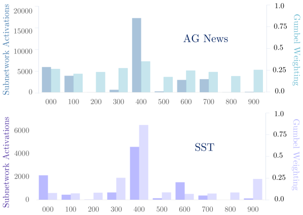
Figure 4: Number of subnetwork activations (classifying words into topics) as well as average Gumbel Softmax activation weights, grouped by Dewey Decimal Subtopic for AG News (top) and SST (bottom).

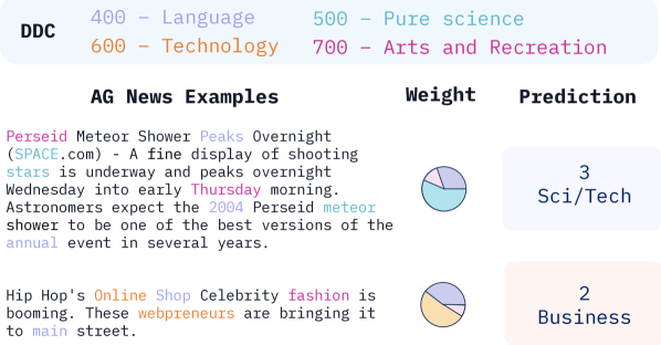
Figure 5: AG News Qualitative examples of interpretability with two articles from AG News. Highlighted text represent an activation from a corresponding DDC subnetwork. The pie chart represents the weighting of each subnetwork in the resultant prediction.

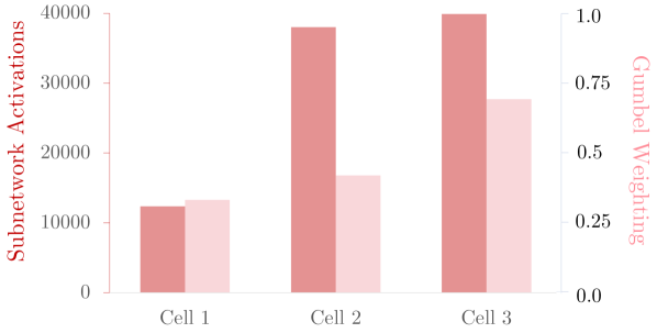
Figure 6: Number of subnetwork activations as well as average Gumbel Softmax activation weights by subnetwork (Cell) for the Breast Cancer dataset.

Influence of Grouping: To illustrate the influence of different feature groupings, we conduct a deep dive for course DSP 1 of the EDU context. Figure 7 illustrates the number of subnetwork activations and corresponding weights for three different groupings.

For the first two groupings (GPT-4, Paper), the subnetwork activations (number of times the route was activated) closely mirror the Gumbel Sigmoid adaptive weighting, indicating that a few networks are activated with high weights for prediction. In the group by GPT-4 setting, we see behaviors of competency, interaction patterns, and assessment frequently activated for student pass-fail predictions. Although ‘interaction patterns‘ is the largest category (most number of features chosen by GPT-4), it still comes second to competency (focusing on student achievement). In the group by paper setting, we see a clear preference for Marras et al. with over $17,500$ students predicted using this network (dark orange) and high weight given to the predictions from the network (light orange).

In contrast, in the third grouping (Pattern), we see a differentiation between the number of activations (dark orange) and the weight of the activations (light orange). Notably, the patterns of ‘Effort‘, ‘Proactivity‘, ‘Consistency‘ and ‘Control‘ all have higher than $50\%$ weight when they are activated, which means they contribute a lot to the overall prediction when chosen.

An in-depth analysis on grouping by paper and pattern over all six courses can be found in Appendix D. We additionally provide a detailed case study on the DSP course using more feature sets and architecture variations.

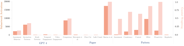
Figure 7: EDU Number of subnetwork activations (left) and Gumbel Softmax activation weights (right) across different groupings (GPT-4, Paper, Pattern) for course DSP 1 of the EDU context.

InterpretCC group routing provides human-centered interpretability without compromsing performance. InterpretCC enables automatic or user-defined grouping and provides adaptation to each data point.

5 Related Work

Conditional Computation (CC) has been proposed to address the time-consuming and computationally expensive training of neural networks by activating only parts of the network (Bengio et al., 2013; Davis & Arel, 2013).
Inspired by the foundations laid out by CC, expert models have rapidly gained popularity for improving both the efficiency and interpretability of neural networks. BASE layers (Lewis et al., 2021) direct each token to a designated expert and Switch Transformers (Fedus et al., 2022b) use Conditional Computation to select one out of four feedforward networks across each transformer layer, optimizing computational resources. LIMoE (Mustafa et al., 2022) further refines this concept by specializing visual experts in identifying distinct concepts such as textures and faces, enriching interpretability. Mixtral (Jiang et al., 2024) is a recent LLM using a mixture of experts to select 2 out of 8 expert networks at each layer at inference, reducing the numbers of parameters used by a factor of 4 compared to training, while allowing each token to have access to all the parameters. InterpretCC is similarly inspired by CC, but we focus on adaptively selecting the number of experts.

Expert models have also been used for global understanding of LLM’s internals. Indeed, through manual inspection of token assignments and expert utilization during inference, it is possible to directly link each expert to specific concepts or features observed in the test set. This analysis reveals a nuanced understanding of expert specialization, from linguistic elements in English LLMs (Lewis et al., 2021) to semantic specializations in multilingual LLMs (Zoph et al., 2022). These insights underscore the adaptability and depth of expert models in contributing to global interpretability. Building on these advances, the Interpretable Mixture of Experts (IME) framework (Ismail et al., 2023) describes and analyses the different approaches to using a mixture of experts for interpretability.

Interpretability based on groups is also explored by the Sum-of-Parts (SOP) model (You et al., 2023), where the prediction process involves making sparse groups of features, highlighting the model’s dependence on subsets of features for its decisions. InterpretCC differentiates from these models by filtering the feature space at the global level using human-understandable concepts.

Other approaches to interpretability use human-understandable concepts (Kim et al., 2017; Ghorbani et al., 2019), or hybrid approaches using both manually defined and unsupervised Concepts (Sawada & Nakamura, 2022). Similar to these approaches, InterpretCC allows users to specify interpretable concepts. However, we do not use examples but instead allow users to specify groupings over the feature space.

6 Conclusion

In this work, we present InterpretCC, a family of interpretable-by-design models that puts interpretability and human understanding at the forefront of the design. Through our experiments in simple, feature gating models and interpretable routing (mixture-of-expert) models, we show comparable performance to baseline approaches.

We provide a model that is optimally interpretable; providing as much interpretation as possible without compromising performance. An atypical student predicted to fail might require 6 features to classify where a regular student predicted to pass might only need 2 markers.

This architecture has limitations, especially grounded in human specification. While expert specification of important feature groupings is crucially needed for actions based on interpretations, it can cause a compromise in performance. Feature gating can also limit important features in a dataset if all features are equally important and minimal (i.e. 10 or less). However, we find that in human-centric applications, the problem is often too many features, not too few.

There is still much experimentation and extension to be done, examining the effects of interpretations downstream in case studies and the ease with which these models can be integrated into applications. We urge the machine community learning to design models for interpretability, as we often are not aware of the many unintended use cases or harmful outcomes of models we have provided.

Impact Statement

This paper presents work whose goal is to advance the field of Machine Learning. There are many potential societal consequences of our work in human-centri, none which we feel must be specifically highlighted here.

Appendix A GPT-4 Routing

To leverage LLMs for automated feature groupings, we use the following prompt alongside the feature descriptions from the appendix table of Swamy et. al (2022a).

Prompt: You are a talented learning scientist, specializing in self-regulated learning behavior. You want to group the following features together into smaller groups of logical concepts based on educational theory with headings. What are your feature groupings?

Response: Certainly, based on educational theory and self-regulated learning behavior, I would group the provided features into the following logical categories:

• Temporal Engagement:

  • DelayLecture

  • RegPeakTimeDayHour

  • RegPeriodicityDayHour

• Study Patterns:

  • NumberOfSessions

  • AvgTimeSessions

  • TotalTimeSessions

  • StdTimeSessions

  • StdTimeBetweenSessions

• Video Engagement:

  • AvgWatchedWeeklyProp

  • StdWatchedWeeklyProp

  • AvgReplayedWeeklyProp

  • StdReplayedWeeklyProp

  • AvgInterruptedWeeklyProp

  • StdInterruptedWeeklyProp

• Competency and Learning Progress:

  • CompetencyStrength

  • CompetencyAlignment

  • CompetencyAnticipation

  • ContentAlignment

  • ContentAnticipation

• Interaction Patterns:

  • TotalClicks

  • TotalClicksProblem

  • TotalClicksVideo

  • TotalClicksWeekday

  • TotalClicksWeekend

  • TotalTimeProblem

  • TotalTimeVideo

  • TotalClicksVideoLoad

  • TotalClicksVideo

  • FrequencyEventVideo

  • FrequencyEventLoad

  • FrequencyEventPlay

  • FrequencyEventPause

  • FrequencyEventStop

  • FrequencyEventSeekBackward

  • FrequencyEventSeekForward

  • FrequencyEventSpeedChange

  • AvgSeekLength

  • StdSeekLength

  • AvgPauseDuration

  • StdPauseDuration

  • AvgTimeSpeedingUp

  • StdTimeSpeedingUp

• Assessment Behavior:

  • StudentSpeed

  • StudentShape

Each grouping represents a different aspect of self-regulated learning behavior, focusing on how students engage with learning resources, interact with content, demonstrate competency, and approach assessments. This categorization aligns with principles of self-regulated learning and can help in analyzing and understanding students’ behaviors and strategies within an educational context.

Appendix B Sparsity Criterion Experiments

For the feature gating architecture to further improve interpretability, we would like the network to learn sparse feature activations. That is, for a given input $x$ we would like to reduce the number of features that affect the model prediction. To achieve this we apply some regularization to the generated feature mask.

One natural choice to enforce sparse feature activations is to apply $L_{1}$-norm regularization to the feature mask, which penalizes a high number of nonzero elements. Another choice is to use annealed regularization as presented by Verelst and Tuytelaars (2019), which might aid the model to first work through a prediction optimization phase that is not confounded by any additional error terms before moving towards a sparsity-enforcing phase.

We experiment with annealing L1 and L1 regularization across six courses, and find that traditional L1 regularization is more stable (at least in the time-series setting). The Baseline BiLSTM results are not reported as confidence intervals here as they are directly sourced from a recent benchmarking paper by Swamy et al., with confirmed similarity by Asadi et al. (2022a; 2023). We reproduce this benchmark above with similar values in 3.

EDU Dataset	Baseline	InterpretCC Feature Gating
40% EP	BiLSTM	Annealing	L1
DSP	82	87.76 +/- 3.12	90.75 +/- 0.01
Geo	76.2	81.13 +/- 5.39	71.92 +/- 0.01
HWTS	72	77.58 +/- 0.01	82.89 +/- 0.04
Structure	52.5	50.00 +/- 0.01	50.00 +/- 0.01
Ventures	51	57.51 +/- 9.12	52.83 +/- 0.03
VA	73.8	84.81 +/- 0.01	77.80 +/- 0.01

Table 6: Annealing L1 regularization in comparison with L1 regularization across 6 course datasets in EDU.

Appendix C Gumbel-SoftMax trick and its application to InterpretCC

To make the feature gating and routing architectures compatible with backpropagation, we need to make the masks differentiable. These discrete decisions can be trained end-to-end using the Gumbel-SoftMax trick (Jang et al., 2017). This method adapts soft decisions into hard ones while enabling backpropagation, i.e. provides a simple way to draw samples from a categorical distribution.

Given a categorical distribution with class probabilities $\pi=[\pi_{1}\,\pi_{2}\,...\,\pi_{N}]$, one can draw discrete samples $z$ as follows:

$$z=\textsc{OneHot}\left(\arg\max_{i}[g_{i}+\log\pi_{i}]\right)$$

where $g_{1}...g_{N}$ are i.i.d. samples drawn from the Gumbel$(0,1)$ distribution. Then, the softmax function is used as a differentiable approximation to $\arg\max$ to generate a $N$-dimensional sample vector $y$ such that

$$y_{i}=\frac{\exp((\log(\pi_{i})+g_{i})/\tau)}{\sum_{j=1}^{N}\exp((\log(\pi_{j})+g_{j})/\tau)}\quad\text{for }i=1,...,N$$

where $\tau$ is a softmax temperature parameter that is fixed at $\tau=1$ for experiments in this project.

Notice that for the gating mechanism, an independent sample is drawn for each ‘gate’ instead of for each datapoint in routing. For example in feature gating, for each feature $i$, a soft-decision $a_{i}\in(-\infty,+\infty)$ is outputted by the discriminator layers. The probability $\pi_{1}$ that the feature should be activated as well as the complement probability $\pi_{2}$ (feature is not activated) can then be computed by using the sigmoid function:

$$\pi_{1}=\sigma(a_{i})\qquad\pi_{2}=1-\pi_{1}=1-\sigma(a_{i})$$

The corresponding (1-dimensional) sample $y$ for each $i$ can thus be reduced to

$$y=\sigma\left(\frac{a_{i}+g_{1}-g_{2}}{\tau}\right)$$

In other words, the discriminator layers from Fig. 1 actually feed into an adapted Gumbel Sigmoid where $\sigma_{i}$ is the corresponding $y$ sample as described above.

For routing (see Fig. 2), the discriminator layers actually output the route logits to a Gumbel SoftMax, which constructs the categorical sample vector (of dimension equal to the number of routes and $i$-th entry $y_{i}$ defined as above).

Finally, we can use a straight-through estimator during training. In other words, binary (or hard/quantized) samples are then used for the forward pass while gradients are obtained from the soft samples for backpropagation. This means that, given soft decisions $\sigma_{i}$, architectures that use a mask $M=[m_{1}\,...\,m_{N}]$ with $m_{i}=\mathds{1}_{\{\sigma_{i}\geq 0.5\}}$ differ in value during the forward and backward pass:

$$m_{i}=\begin{cases}\mathds{1}_{\{\sigma_{i}\geq 0.5\}}\qquad\text{(forward pass)},\\ \sigma_{i}\qquad\qquad\quad\text{(backward pass)}\end{cases}$$

Appendix D Additional Analyses: EDU

Some additional analyses regarding the education InterpretCC routing models.

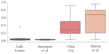
Figure 8: EDU Which route was taken? This is an analysis of group by paper routing averaged over all six courses for each paper grouping. The y-axis represents the proportion of points for which the subnetwork is activated.

In Figure 8, we see InterpretCC routing by research paper (grouping the features based on the paper they were proposed in). The Marras et al. and Chen Cui feature sets have clearly been identified as important over the majority of courses, echoing findings in other learning science literature using BiLSTM and random forest architectures (Marras et al., 2021; Chen & Cui, 2020; Swamy et al., 2023a). The large standard deviations in the box-plots indicate that for at least some courses (in this case Structures and Venture), Chen Cui and Marras were not found significantly important. Notably, the same courses that have low accuracies on routing in 3 are those that have low scores on the two most popular feature sets, showing a consensus among performant InterpretCC models and a validation of the identification of importance.

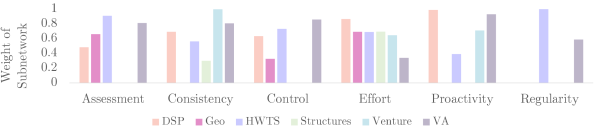
Figure 9: EDU Weighting distribution across subnetworks grouped by pattern for 6 courses.

In Fig. 9, we see a widely varying distribution of patterns selected across courses, showcasing the ability of InterpretCC to adaptively select subnetwork weights depending on the dataset.

Appendix E Case Study: DSP 1

In the following appendix section, we conduct a detailed case study for DSP 1 (Digital Signal Processing), a well-researched course in the learning science community (2016; 2022a). We extend the analysis from 4 papers of feature groups (45 features) to 10 papers of feature groups (97 features) (Lallé & Conati, 2020; Boroujeni et al., 2016; Chen & Cui, 2020; Marras et al., 2021; He et al., 2018; Lemay & Doleck, 2020; Mbouzao et al., 2020; Mejia et al., 2022; Mubarak et al., 2021; Wan et al., 2019).

Baseline Architectures The results in Table 7 provide a target performance for subsequent architectures. One might expect a tradeoff between gaining higher interpretability and lowering performance; however, the objective is to maintain similar predictive performance with an interpretable design.

Early prediction	Accuracy	Balanced Accuracy	ROC AUC
40%	0.835	0.653	0.858
60%	0.944	0.925	0.982

Table 7: Baseline model test performance metrics for both 40% and 60% early success prediction settings

Feature Gating First, a nice result for the feature gating architectures is that balanced accuracy is not only maintained but is actually improved upon compared to the baseline (see Table 8 for full model results). A maximum of 0.770 and 0.935 balanced accuracy is reached for the 40 and 60 percent settings respectively (compared to 0.653 and 0.925 baseline).

Setting	Model	Performance  ACC  BAC AUC	Activated Features $\;\;\;\mu\;\;\;$ $\,\,\;\sigma\;\,\,$
40%	Baseline L1 (1e-5) L1 (1e-4) Annealed MSE Truncated AMSE	0.835 0.653 0.858 0.790 0.711 0.817 0.763 0.748 0.784 0.768 0.770 0.823 0.805 0.743 0.823	97 0 8.54 0.58 2.20 1.64 13.26 3.72 5.95 1.03
60%	Baseline L1 (1e-5) L1 (1e-4) Annealed L1 (1e-5) Annealed MSE Truncated AMSE	0.944 0.925 0.982 0.914 0.935 0.963 0.914 0.917 0.957 0.910 0.927 0.957 0.892 0.927 0.952 0.787 0.788 0.839	97 0 37.60 3.97 31.38 4.45 38.36 3.61 21.45 3.23 - -

Table 8: Feature Gating - test performance metrics comparison between different sparsification methods next to their average and standard deviation of number of activated features for both 40% and 60% early success prediction settings; baseline benchmarks also provided for contrast.

An annealed mean-squared regularization proved most effective for the 40% setting, although it activated more features on average than $L_{1}$-norm regularization which more effectively reduced the feature space while achieving desirable balanced accuracy performance in this setting. By truncating the initial feature space to only the activated features and using the same architecture, performance is almost maintained even though the average number of activated features per datapoint is more than halved (from around 13 to 6). This method was not as effective for the 60% setting however. Truncating the feature space largely reduces predictive capability (e.g. almost a 0.15 drop in balanced accuracy). L1 regularization in this case proved best. Using an annealed regularization did not significantly improve or change model performance as well.

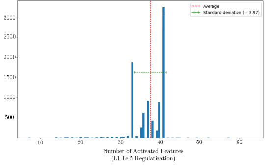
Figure 10: Feature gating (60% setting & L1(1e-5) regularization) - Number of activated routes distribution.

Next, experiments have also shown that the feature gating architecture successfully learns a dynamic feature activation mask (e.g. see Fig. 10). Interestingly, not all features are selected at least once, rather the activated features form a subset from the initial input set. There is large overlap and similarity in selected features regardless of sparsity criterion method. For example, in the 40% setting the most popular features that are almost always activated are total video load clicks, total video clicks, time between sessions statistics, total problem solving time, student speed, as well as competency strength. In the 60% setting, student speed and total problem solving time, as well as time between sessions statistics remain highly activated features.

Finally, to determine whether this dynamic feature activation is useful to increase model performance, we compare to a BiLSTM network that fixes the top $k$ activated features as input where $k=\left\lceil{\mu}\right\rceil$ is equal to the average number of active features rounded up. Balanced accuracy ends up slightly worse for both early prediction settings (0.64 and 0.91 respectively) thus there are above marginal gains to be gained from using dynamic feature selections.

Easy-hard Routing The easy-hard routing architecture performs on-par with the baseline in terms of accuracy and even slightly improves upon balanced accuracy (see Table 9). Interpretability gains, however, are marginal as only a small minority of datapoints pass through the ‘easy’ route for both prediction settings. This means there is only a minor interpretable advantage of having a reduced input feature space.

Early prediction	Accuracy	Balanced accuracy
40%	0.85	0.68
60%	0.95	0.93

Table 9: Easy-Hard routing - model test performance metrics for the 40% and 60% early prediction settings

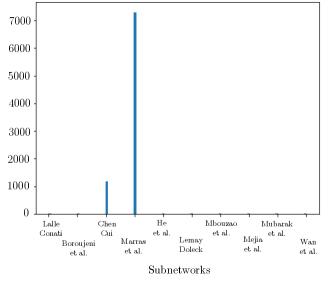
Figure 11: Pretrained routing - route choices

Routing by pattern Unfortunately the routing by pattern method was unable to confidently surpass 0.5 balanced accuracy for both early prediction settings. This is most likely due to the fact that the feature groupings are too small (at most 3 per route) given their current construction. However, one should further consider building larger feature groupings upon them in order for the sub-networks to gain independent predictive power. Here we have observed a limitation of the routing architecture: the overall model performance is heavily limited by the independent performance of the sub-networks. If the feature subsets passed as input are insufficient for the model to learn how to confidently predict all outcome classes, then there is no practical interpretability to gain. For example, in this routing case, the black-box model is a uniform class predictor (i.e. only outputs the same label) thus there is no sense in explaining its decisions as it cannot discriminate between the outcome classes. In summary, the routing architecture’s performance and utility is limited by the predictive quality of the chosen feature groupings.

Routing by paper In contrast to routing by pattern, the routing by paper experiments have shown performance that approximately matches the baseline target (see Table 10). The 40% model is slightly less effective than the balanced accuracy benchmark (0.621 versus 0.653) while the 60% version slightly surpasses it (0.935 versus 0.925).

Early prediction	Accuracy	Balanced accuracy	ROC AUC
40%	0.850	0.621	0.851
60%	0.940	0.935	0.976

Table 10: Routing by paper - model test performance metrics for the 40% and 60% early success prediction settings

The network chooses for a majority of datapoints to proceed with the ‘Marras et al.’ route for both settings. The ‘Chen and Cui’ route is given slight importance for 60% early prediction as well. More striking is that, by inspecting how the other routes fare on unseen data when activated, they precisely predict the outcome class with a 100% accuracy. Although this only concerns a minor portion of datapoints (between 2.5 to 5 percent of data) and should be further inspected, a possibility is that the concerned routes might identify a pattern or value in their input features that indicates with certainty the correct outcome label. This is incredibly helpful in terms of explainability as one might more easily pinpoint how the model came to its decision. Moreover, this model seemed to have identified the feature group with the best predictive capability (in this case ‘Marras et al.’) to which to send all unsure datapoints. Route activations might give an indication of feature importance, similarly to feature gating. Moreover, predictions are also made on a smaller input feature space which arguably increases interpretability. Overall, this method has promising results and behaviour which maintains benchmark performance and helps output explanations.

Routing by paper with pretrained sub-networks achieves 0.937 accuracy, 0.918 balanced accuracy, and 0.976 ROC AUC in the 60% setting. The individual test performance of the frozen sub-networks, as well as their number of input features and activation percentage are noted in Table 11.

Paper	# of features	% activated	Accuracy	Balanced accuracy	ROC AUC
Lallé and Conati	22	0.003	0.885	0.725	0.867
Boroujeni et al.	3	0.003	0.858	0.711	0.830
Chen and Cui	13	0.137	0.918	0.871	0.965
Marras et al.	7	0.840	0.941	0.923	0.979
He et al.	3	0.003	0.824	0.500	0.478
Lemay and Doleck	10	0.003	0.824	0.500	0.497
Mbouzao et al.	3	0.002	0.824	0.500	0.504
Mejia et al.	10	0.003	0.824	0.500	0.482
Mubarak et al.	13	0.003	0.824	0.500	0.534
Wan et al.	13	0.002	0.824	0.500	0.478

Table 11: Test performance of all pretrained sub-networks, along with their corresponding number of input features, and activation percentage when used in routing

All feature groupings below ‘Marras et al.’ in Table 11 have a balanced accuracy of 0.5. In other words, by taking such standalone feature groups as input, the current expert sub-network architecture is unable to discriminate between a passing or failing student, and performs no better than a uniform or random class predictor.

Routing in this case similarly activates in majority the ‘Marras et al.’ and ‘Chen and Cui’ routes just like normal routing. The notable result here is to notice that using pretrained sub-networks does not necesarily improve nor change the model behaviour. Thus it is not necessary to add an expert pre-training step to the model pipeline, and the model can optimize its sub-networks as well as learn the dynamic routing simultaneously during training.

Gated routing The gated routing alternative architecture (which takes the average of all activated routes’ predictions as output) does not perform as well as weighted routing (see Table 12) regardless of route sparsity criterion. However, once again routes are similarly activated across methods (see Table 13). Once again, the same ‘Marras et al.’ and ‘Chen and Cui’ routes are heavily favored with them being activated for every datapoint (along with the ‘Boroujeni et al.’ path). This architecture thus can also help outline feature group importance, although not as effectively as single-route routing.

Regularization	# of routes $\mu\pm\sigma$	Accuracy	Balanced accuracy	ROC AUC
L1	$4.64\pm 0.82$	0.901	0.788	0.960
Annealed L1	$3.92\pm 0.81$	0.902	0.807	0.959
Annealed MSE	$4.22\pm 0.89$	0.899	0.789	0.959

Table 12: Gated routing models performance comparison for different regularization methods along with the corresponding average and standard deviation of activated routes

Paper	% activated     L1 AL1 AMSE
Lallé and Conati Boroujeni et al. Chen and Cui Marras et al. He et al. Lemay and Doleck Mbouzao et al. Mejia et al. Mubarak et al. Wan et al.	0.535 0.252 0.523 1.000 1.000 1.000 1.000 1.000 1.000 1.000 1.000 1.000 0.001 0.000 0.023 0.000 0.000 0.000 0.000 0.000 0.000 0.751 0.449 0.098 0.000 0.000 0.000 0.352 0.220 0.578

Table 13: Gated routing - route activation percentage statistics for different sparsification methods ($L_{1}$-norm (L1), annealed $L_{1}$-norm (AL1), and annealed mean-squared error (AMSE))

Weighted routing Finally, the weighted group routing design yields the best performance seen so far, with balanced accuracy reaching 0.94 for a threshold of 0.005 (see Table 14). For all tested thresholds, accuracy remains at similar levels above the baseline performance, and differ mostly in the number of routes that are activated. For example, for a threshold of 0.005 there are an average of 2.35 activated routes with a standard deviation of 2.80 compared to $1.29\pm 0.55$ for a threshold of 0.1. Logically a higher threshold leads to a lower number of activated routes; therefore, one might consider the tradeoff between choosing a higher threshold for less computation power required at inference. In this case, the difference in predictive performance between a high and low threshold is almost negligible thus one should prefer minimizing the number of considered routes (for interpretability reasons as well as it is easier to consider a smaller subset of features).

Threshold	# of Routes $\mu\pm\sigma$	Accuracy	Balanced accuracy	ROC AUC
None ($\geq 0$)	$10\pm 0$	0.947	0.934	0.983
$\geq 0.005$	$2.35\pm 2.80$	0.950	0.939	0.984
$\geq 0.01$	$1.69\pm 1.55$	0.947	0.927	0.982
$\geq 0.05$	$1.27\pm 0.50$	0.940	0.935	0.982
$\geq 0.1$	$1.29\pm 0.55$	0.949	0.936	0.980

Table 14: Group weighted routing models test performance comparison for different thresholds along with their corresponding average and standard deviation of activated routes

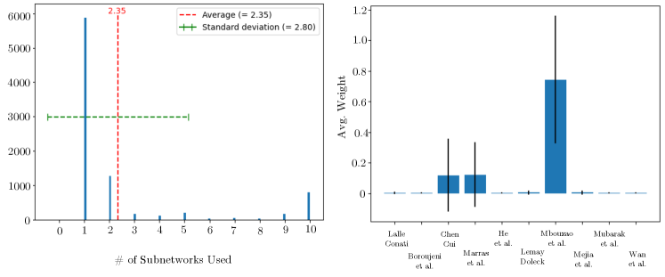
Figure 12: Group weighted routing threshold = 0.005 (left) Distribution of the number of activated routes. (right) Average route weights with standard deviation error bars.

We further look into how the routes are weighted for the best performing model (see Figure 12). At first glance, it seems that the model highly values the ‘Mbouzao et al.’ route, above the ‘Chen and Cui’ and ‘Marras et al.’ paths, which was previously not the case in other routing alternatives. However upon further inspection, the ‘Mbouzao’ path always suggests the same outcome label (fail) when activated. This means that when the model activates this path, it likely believes the given student belongs to the fail class. Thus it is normal that the average weight of this route is high since there is a strong class imbalance in favor of the latter outcome. This is very interesting from an interpretability point of view as we can understand the weighting of this path as a confidence score that a student will fail. Moreover, a higher weight of the ‘Marras’ and ‘Chen-Cui’ routes can be thought of as the model giving more importance to expert predictors when unsure of the outcome. This also comes at a disadvantage; that is, route weights cannot be easily correlated to feature importance. Another path instead of ‘Mbouzao’ might have been chosen under another model initialization, such as the ‘Mubarak’ route which also uniformly predicts the fail class. Thus one should consider differences from models built with different initialization seeds before coming to conclusions on feature importances. Overall, this weighting behaviour further improves understanding of the model decisions while providing excellent predictive performance.

Route	% activated	Route weight $\mu\pm\sigma$
Lallé and Conati	0.125	$0.002\pm 0.006$
Boroujeni et al.	0.113	$0.002\pm 0.005$
Chen and Cui	0.270	$0.118\pm 0.238$
Marras et al.	0.322	$0.121\pm 0.212$
He et al.	0.114	$0.002\pm 0.005$
Lemay and Doleck	0.159	$0.005\pm 0.014$
Mbouzao et al.	0.863	$0.742\pm 0.417$
Mejia et al.	0.144	$0.004\pm 0.012$
Mubarak et al.	0.124	$0.002\pm 0.005$
Wan et al.	0.115	$0.002\pm 0.005$

Table 15: Weighed routing (threshold = 0.005) - route activation statistics for (1) percentage activated; (2) average and standard deviation route weights

References

- Achiam et al. (2023) Achiam, J., Adler, S., Agarwal, S., Ahmad, L., Akkaya, I., Aleman, F. L., Almeida, D., Altenschmidt, J., Altman, S., Anadkat, S., et al. GPT-4 technical report. arXiv preprint arXiv:2303.08774, 2023.
- Asadi et al. (2022) Asadi, M., Swamy, V., Frej, J., Vignoud, J., Marras, M., and Käser, T. Ripple: Concept-based interpretation for raw time series models in education. In Proceedings of the 13th AAAI Symposium on Educational Advances in Artificial Intelligence, 2022. Accepted as a full paper at AAAI 2023: 37th AAAI Conference on Artificial Intelligence (EAAI: AI for Education Special Track), 7-14 of February 2023, Washington DC, USA.
- Asadi et al. (2023) Asadi, M., Swamy, V., Frej, J., Vignoud, J., Marras, M., and Käser, T. Ripple: Concept-based interpretation for raw time series models in education. In Proceedings of the AAAI Conference on Artificial Intelligence, 2023.
- Bengio et al. (2015) Bengio, E., Bacon, P.-L., Pineau, J., and Precup, D. Conditional computation in neural networks for faster models, 2015.
- Bengio et al. (2013) Bengio, Y., Léonard, N., and Courville, A. C. Estimating or propagating gradients through stochastic neurons for conditional computation, 2013.
- Boroujeni et al. (2016) Boroujeni, M. S., Sharma, K., Kidziński, Ł., Lucignano, L., and Dillenbourg, P. How to quantify student’s regularity? In Verbert, K., Sharples, M., and Klobučar, T. (eds.), Adaptive and Adaptable Learning, pp. 277–291, Cham, 2016. Springer International Publishing. ISBN 978-3-319-45153-4.
- Chen et al. (2019) Chen, C., Li, O., Tao, D., Barnett, A., Rudin, C., and Su, J. K. This looks like that: deep learning for interpretable image recognition. Advances in neural information processing systems, 32, 2019.
- Chen & Cui (2020) Chen, F. and Cui, Y. Utilizing student time series behaviour in learning management systems for early prediction of course performance. Journal of Learning Analytics, 7(2):1–17, 9 2020.
- Davis & Arel (2013) Davis, A. and Arel, I. Low-rank approximations for conditional feedforward computation in deep neural networks, 2013.
- Devlin et al. (2018) Devlin, J., Chang, M.-W., Lee, K., and Toutanova, K. Bert: Pre-training of deep bidirectional transformers for language understanding. arXiv preprint arXiv:1810.04805, 2018.
- Dhurandhar et al. (2018) Dhurandhar, A., Chen, P.-Y., Luss, R., Tu, C.-C., Ting, P., Shanmugam, K., and Das, P. Explanations based on the missing: Towards contrastive explanations with pertinent negatives. In Proceedings of the 32nd International Conference on Neural Information Processing Systems, NIPS’18, pp. 590–601, Red Hook, NY, USA, 2018. Curran Associates Inc.
- Fedus et al. (2022a) Fedus, W., Dean, J., and Zoph, B. A review of sparse expert models in deep learning. arXiv preprint arXiv:2209.01667, 2022a.
- Fedus et al. (2022b) Fedus, W., Zoph, B., and Shazeer, N. Switch transformers: Scaling to trillion parameter models with simple and efficient sparsity. The Journal of Machine Learning Research, 23(1):5232–5270, 2022b.
- Ghorbani et al. (2019) Ghorbani, A., Wexler, J., Zou, J., and Kim, B. Towards automatic concept-based explanations, 2019.
- He et al. (2018) He, H., Zheng, Q., Dong, B., and Yu, H. Measuring student’s utilization of video resources and its effect on academic performance. In 2018 IEEE 18th International Conference on Advanced Learning Technologies (ICALT), pp. 196–198, 2018.
- HF Canonical Model Maintainers (2022) HF Canonical Model Maintainers. distilbert-base-uncased-finetuned-sst-2-english (revision bfdd146), 2022.
- Ismail et al. (2023) Ismail, A. A., Arik, S. O., Yoon, J., Taly, A., Feizi, S., and Pfister, T. Interpretable mixture of experts. Transactions on Machine Learning Research, 2023.
- Jang et al. (2017) Jang, E., Gu, S., and Poole, B. Categorical reparameterization with gumbel-softmax. In International Conference on Learning Representations, 2017.
- Jiang et al. (2024) Jiang, A. Q., Sablayrolles, A., Roux, A., Mensch, A., Savary, B., Bamford, C., Chaplot, D. S., Casas, D. d. l., Hanna, E. B., Bressand, F., et al. Mixtral of experts. arXiv preprint arXiv:2401.04088, 2024.
- Kim et al. (2017) Kim, B., Wattenberg, M., Gilmer, J., Cai, C., Wexler, J., Viegas, F., and Sayres, R. Interpretability beyond feature attribution: Quantitative testing with concept activation vectors (tcav). ICML 2018, 2017.
- Krishna et al. (2022) Krishna, S., Han, T., Gu, A., Pombra, J., Jabbari, S., Wu, S., and Lakkaraju, H. The disagreement problem in explainable machine learning: A practitioner’s perspective. arXiv preprint arXiv:2202.01602, 2022.
- Lallé & Conati (2020) Lallé, S. and Conati, C. A data-driven student model to provide adaptive support during video watching across moocs. In Bittencourt, I. I., Cukurova, M., Muldner, K., Luckin, R., and Millán, E. (eds.), Artificial Intelligence in Education, pp. 282–295, Cham, 2020. Springer International Publishing. ISBN 978-3-030-52237-7.
- Lemay & Doleck (2020) Lemay, D. J. and Doleck, T. Grade prediction of weekly assignments in moocs: mining video-viewing behavior. Education and Information Technologies, 25(2):1333–1342, 2020.
- Lewis et al. (2021) Lewis, M., Bhosale, S., Dettmers, T., Goyal, N., and Zettlemoyer, L. Base layers: Simplifying training of large, sparse models. In International Conference on Machine Learning, pp. 6265–6274. PMLR, 2021.
- Li et al. (2022) Li, M., Gururangan, S., Dettmers, T., Lewis, M., Althoff, T., Smith, N. A., and Zettlemoyer, L. Branch-train-merge: Embarrassingly parallel training of expert language models. arXiv preprint arXiv:2208.03306, 2022.
- Lundberg & Lee (2017) Lundberg, S. M. and Lee, S.-I. A unified approach to interpreting model predictions. In Proceedings of the 31st International Conference on Neural Information Processing Systems, NIPS’17, pp. 4768–4777, Red Hook, NY, USA, 2017. Curran Associates Inc. ISBN 9781510860964.
- Marras et al. (2021) Marras, M., Tu, T., Vignoud, J., and Käser, T. Can feature predictive power generalize? benchmarking early predictors of student success across flipped and online courses. Proceedings of the 14th International Conference on Educational Data Mining, 2021.
- Mbouzao et al. (2020) Mbouzao, B., Desmarais, M. C., and Shrier, I. Early prediction of success in mooc from video interaction features. In Bittencourt, I. I., Cukurova, M., Muldner, K., Luckin, R., and Millán, E. (eds.), Artificial Intelligence in Education, pp. 191–196, Cham, 2020. Springer International Publishing. ISBN 978-3-030-52240-7.
- Mejia et al. (2022) Mejia, P., Marras, M., Giang, C., and Käser, T. Identifying and comparing multi-dimensional student profiles across flipped classrooms. In Artificial Intelligence in Education Proceedings, volume Part I of Lecture Notes in Computer Science. 13355, pp. 90–102. Springer, 2022.
- Miller (2019) Miller, T. Explanation in artificial intelligence: Insights from the social sciences. Artificial intelligence, 267:1–38, 2019.
- Mubarak et al. (2021) Mubarak, A. A., Cao, H., and Ahmed, S. A. Predictive learning analytics using deep learning model in moocs’ courses videos. Education and Information Technologies, 26:371–392, 2021.
- Mustafa et al. (2022) Mustafa, B., Riquelme, C., Puigcerver, J., Jenatton, R., and Houlsby, N. Multimodal contrastive learning with limoe: the language-image mixture of experts. Advances in Neural Information Processing Systems, 35:9564–9576, 2022.
- Nauta et al. (2023) Nauta, M., Schlötterer, J., van Keulen, M., and Seifert, C. Pip-net: Patch-based intuitive prototypes for interpretable image classification. In Proceedings of the IEEE/CVF Conference on Computer Vision and Pattern Recognition, pp. 2744–2753, 2023.
- Reimers & Gurevych (2019) Reimers, N. and Gurevych, I. Sentence-bert: Sentence embeddings using siamese bert-networks. arXiv preprint arXiv:1908.10084, 2019.
- Ribeiro et al. (2016) Ribeiro, M. T., Singh, S., and Guestrin, C. ”why should i trust you?”: Explaining the predictions of any classifier. 22nd ACM SIGKDD International Conference on Knowledge Discovery and Data Mining, pp. 1135–1144, 2016.
- Satija (2013) Satija, M. P. The theory and practice of the Dewey decimal classification system. Elsevier, 2013.
- Sawada & Nakamura (2022) Sawada, Y. and Nakamura, K. Concept bottleneck model with additional unsupervised concepts. IEEE Access, 10:41758–41765, 2022.
- Scott & SCOTT (1998) Scott, M. L. and SCOTT, M. L. Dewey decimal classification. Libraries Unlimited, 1998.
- Selvaraju et al. (2019) Selvaraju, R. R., Cogswell, M., Das, A., Vedantam, R., Parikh, D., and Batra, D. Grad-CAM: Visual explanations from deep networks via gradient-based localization. International Journal of Computer Vision, 128(2):336–359, 10 2019.
- Socher et al. (2013) Socher, R., Perelygin, A., Wu, J., Chuang, J., Manning, C. D., Ng, A. Y., and Potts, C. Recursive deep models for semantic compositionality over a sentiment treebank. In Proceedings of the 2013 conference on empirical methods in natural language processing, pp. 1631–1642, 2013.
- Swamy et al. (2022a) Swamy, V., Marras, M., and Käser, T. Meta transfer learning for early success prediction in moocs. In Proceedings of the Ninth ACM Conference on Learning@ Scale, pp. 121–132, 2022a.
- Swamy et al. (2022b) Swamy, V., Marras, M., and Käser, T. Meta transfer learning for early success prediction in moocs, 2022b.
- Swamy et al. (2022c) Swamy, V., Radmehr, B., Krco, N., Marras, M., and Käser, T. Evaluating the explainers: Black-box explainable machine learning for student success prediction in MOOCs. In Mitrovic, A. and Bosch, N. (eds.), Proceedings of the 15th International Conference on Educational Data Mining, pp. 98–109, Durham, United Kingdom, 7 2022c. International Educational Data Mining Society. ISBN 978-1-7336736-3-1.
- Swamy et al. (2023a) Swamy, V., Du, S., Marras, M., and Kaser, T. Trusting the explainers: teacher validation of explainable artificial intelligence for course design. In LAK23: 13th International Learning Analytics and Knowledge Conference, pp. 345–356, 2023a.
- Swamy et al. (2023b) Swamy, V., Frej, J., and Käser, T. The future of human-centric explainable artificial intelligence (xai) is not post-hoc explanations. arXiv preprint arXiv:2307.00364, 2023b.
- Verelst & Tuytelaars (2019) Verelst, T. and Tuytelaars, T. Dynamic convolutions: Exploiting spatial sparsity for faster inference, 2019.
- Wan et al. (2019) Wan, H., Liu, K., Yu, Q., and Gao, X. Pedagogical intervention practices: Improving learning engagement based on early prediction. IEEE Transactions on Learning Technologies, 12(2):278–289, 2019.
- Wolberg et al. (1995) Wolberg, W., Olvi, M., Street, N., and Street, W. Breast Cancer Wisconsin (Diagnostic). UCI Machine Learning Repository, 1995. DOI: https://doi.org/10.24432/C5DW2B.
- Yang et al. (2019) Yang, Z., Dai, Z., Yang, Y., Carbonell, J., Salakhutdinov, R. R., and Le, Q. V. Xlnet: Generalized autoregressive pretraining for language understanding. Advances in neural information processing systems, 32, 2019.
- You et al. (2023) You, W., Qu, H., Gatti, M., Jain, B., and Wong, E. Sum-of-parts models: Faithful attributions for groups of features. arXiv preprint arXiv:2310.16316, 2023.
- Zhang et al. (2015) Zhang, X., Zhao, J., and LeCun, Y. Character-level convolutional networks for text classification. Advances in neural information processing systems, 28, 2015.
- Zoph et al. (2022) Zoph, B., Bello, I., Kumar, S., Du, N., Huang, Y., Dean, J., Shazeer, N., and Fedus, W. Designing effective sparse expert models. arXiv preprint arXiv:2202.08906, 2, 2022.