A subspace method for large-scale trace ratio problems

Abstract

We present a subspace method to solve large-scale trace ratio problems. This method is matrix-free, only needing the action of the two matrices in the trace ratio. At each iteration, a smaller trace ratio problem is addressed in the search subspace. Additionally, our algorithm is endowed with a restarting strategy, that ensures the monotonicity of the trace ratio value throughout the iterations. We also investigate the behavior of the approximate solution from a theoretical viewpoint, extending existing results on Ritz values and vectors, as the angle between the search subspace and the exact solution to the trace ratio approaches zero. In the context of multigroup classification, numerical experiments show that the new subspace method tends to be more efficient than iterative approaches that need a (partial) eigenvalue decomposition in every step.

1 Introduction

Let $A$ and $B$ be $p\times p$ matrices, where $A$ is symmetric and $B$ is symmetric positive definite (SPD). Let $V$ be $p\times k$, with orthonormal columns, and $I_{k}$ be the $k\times k$ identity matrix. We develop and investigate a subspace method for the trace ratio optimization problem (TR, cf. [17])

(1) $$\max_{V^{T}V=I_{k}}\rho(V):=\frac{\mathop{{\rm tr}}(V^{T}\!AV)}{\mathop{{\rm tr}}(V^{T}\!BV)},$$

where $\mathop{{\rm tr}}(\cdot)$ indicates the trace of a matrix; $I_{k}$ is the $k\times k$ identity matrix. The TR problem has often been studied as an alternative method to Fisher’s discriminant analysis (FDA, see, e.g., [10, Ch. 11]) for dimensionality reduction and classification of multigroup data (cf. Section 5). For FDA, the problem of interest is the maximization of the trace of a ratio, which has the equivalent forms (cf. [1, Prop. 2.1.1]):

(2) $$\max_{V^{T}\!BV=I_{k}}\mathop{{\rm tr}}(V^{T}\!AV)=\max_{{\rm rank}(V)=k}\mathop{{\rm tr}}((V^{T}\!BV)^{-1}\,V^{T}\!AV),$$

where ${\rm rank}(\cdot)$ indicates the rank of a matrix. The maximizer of this problem is given by the $k$ generalized eigenvectors of the pair $(A,B)$, corresponding to the $k$ largest eigenvalues (see, e.g., [17]). Therefore, finding the solution to FDA is equivalent to solving the generalized eigenvalue problem (GEP) $A\mathbf{x}=\lambda B\mathbf{x}$, for its $k$ largest eigenvalues.

In general, TR does not have a closed-form solution. A typical Newton type iterative method to solve (1) consists of solving a sequence of eigenvalue problems, where, at each iteration, the $k$ leading eigenvectors are required. In a context where $p$ is large, subspace methods are preferable to (dense) methods solving all eigenpairs. In [34, 17], the implicitly restarted Lanczos method is employed for this task. Regarding the GEP (and also FDA), there exist several methods to retrieve the $k$ leading generalized eigenvectors from $(A,B)$, where $A$ is symmetric and $B$ is SPD; for instance, Davidson type methods (see, e.g., [2] or [20, Sec. 8.3]), LOBPCG [11], or Jacobi–Davidson approaches for hard cases with clustered eigenvalues [22].

Inspired by Davidson type methods, we propose a subspace method for solving the TR problem. The idea is to produce a suitable search subspace by solving a sequence of trace ratio problems after projecting $A$ and $B$. A residual matrix is then used to enrich the search subspace, and a suitable restarting technique is exploited to lower both the computational cost and the memory requirements. Finally, this method is especially convenient if $A$ and $B$ are sparse, or the matrix-vector multiplications by $A$ and $B$ are cheap to compute. In the context of multigroup classification, both $A$ and $B$ can be factored in a convenient way (see, e.g., [34]), making TR and FDA ideal candidates for subspace methods.

The paper is organized as follows. Section 2 gives an overview of the trace ratio problem, its properties, and the commonly used iterative method to find its solution. Section 3 describes the three phases of a new Davidson type method to solve TR: extraction, expansion, and restart. We show that the iterations of our algorithm generate a non-decreasing sequence of trace ratio values. Section 4 discusses the behavior of the approximate solution generated by the subspace method, and the related approximate eigenvalues, under the hypothesis that the angle between the search subspace and the exact solution approaches zero. In Section 5, we review TR and FDA in the context of multigroup classification. A Davidson’s method for solving FDA is proposed in Section 5.1. This is already known in the context of subspace methods for eigenvalue problems, but we provide some further insight on the restarting mechanism. The two TR algorithms and Davidson’s method for FDA are applied to multigroup classification in Section 6, and tested on both synthetic and real datasets. Conclusions are drawn in Section 7.

We denote the eigenvalues of symmetric matrix $A$ by $\lambda_{1}(A)\geq\cdots\geq\lambda_{p}(A)$. Similarly, $\lambda_{1}(A,B)\geq\cdots\geq\lambda_{p}(A,B)$ are the eigenvalues of the pair $(A,B)$, where $A$ is symmetric and $B$ is SPD. The Frobenius norm of a matrix and the Euclidean norm of a vector, are indicated with $\|\cdot\|$; the spectral norm of a matrix is $\|\cdot\|_{2}$; $\|\mathbf{x}\|_{A}^{2}=\mathbf{x}^{T}\!A\mathbf{x}$ is used for the $A$-weighted norm of an SPD matrix $A$.

2 Overview of the trace ratio problem

In this section, we recall some properties of the trace ratio problem and report the well-known iterative method to find its solution. The trace ratio problem is well defined, under the appropriate hypotheses on $(A,B)$, since it admits a finite solution [17, Prop. 3.2]:

Proposition 1.

Let $A$ be symmetric and $B$ be symmetric positive semidefinite, with ${\rm rank}(B)\geq p-k+1$. Then (1) admits a finite maximum.

Let $\rho^{\ast}$ be the global maximizer of (1). Then, a necessary condition for $V^{\ast}$ to be a corresponding maximizer is (cf. [17, Eq. (4.1)])

(3) $$\max_{V^{T}V=I_{k}}\mathop{{\rm tr}}(V^{T}(A-\rho^{\ast}B)\,V)=\mathop{{\rm tr}}((V^{\ast})^{T}(A-\rho^{\ast}B)\,V^{\ast})=0.$$

From the Courant–Fischer characterization (see, e.g., [17]), $V^{\ast}$ is an orthonormal basis for the eigenspace of $A-\rho^{\ast}B$, associated with its $k$ largest eigenvalues.

A direct consequence of (3) is formulated in [21, Thm. 2], which states that every local maximizer is also a global one. Moreover, [34, Thm. 3.4] shows that the condition (3) is also sufficient. We hereby report its statement:

Proposition 2.

Let $\rho^{\ast}$ be the global maximum of (1). Then any $V^{\ast}$ is a global maximizer for (1) if and only if it is an orthonormal basis for the eigenspace of the matrix $A-\rho^{\ast}B$, corresponding to its $k$ largest eigenvalues. In addition, $\mathop{{\rm tr}}((V^{\ast})^{T}(A-\rho^{\ast}B)V^{\ast})=0$.

Uniqueness (up to orthonormal transformations) is also discussed in, e.g., [21, 34, 17]. From [34, Thm. 3.4], the solution to (1) is spanned by the $k$ leading eigenvectors of $A-\rho^{\ast}B$. This subspace is unique if there is a gap between the $k$th and the $(k+1)$st largest eigenvalues, i.e., $\lambda_{k}(A-\rho^{\ast}B)>\lambda_{k+1}(A-\rho^{\ast}B)$. In this situation, the solution is uniquely described by the set $\{VQ\,:\,Q\in\mathbb{R}^{k\times k},\,Q^{T}Q=I_{k}\}$. When there is no gap, we still retain the uniqueness of $\rho^{\ast}$, as a consequence of Proposition 2. We also provide a small example.

Example 3.

Let $A={\rm diag}(3,2,1)$, $B={\rm diag}(1,4,3)$, $k=2$. One may check that the maximum trace ratio is $\rho^{\ast}=1$, with $A-\rho^{\ast}B={\rm diag}(2,-2,-2)$. The maximizing subspace is spanned by the first canonical basis vector $\mathbf{e}_{1}$, and any linear combination of $\mathbf{e}_{2}$ and $\mathbf{e}_{3}$.

Starting from (3), the trace ratio problem (1) can be recast as a root-finding problem [17]. Specifically, in view of (3), we look for a zero of $f(\rho)=\max_{V^{T}V=I_{k}}\mathop{{\rm tr}}(V^{T}(A-\rho B)V)$. A common iterative method to find it is a Newton type method, summarized in Algorithm 1. The method may also be viewed as member of the family of self-consistent field methods (see, e.g., [33], where a generalization of the trace ratio function is studied).

Algorithm 1 Iterative method to solve the trace ratio problem (1)

Input: Symmetric $A\in\mathbb{R}^{p\times p}$, SPD $B\in\mathbb{R}^{p\times p}$, dimension $k<p$; (optional) initial trace ratio value $\rho_{0}$, tolerance tol.
Output: $(p\times k)$ minimizer $V$ with maximum $\rho$.
1: If $\rho_{0}$ is not provided: 2:   M Select random $n\times k$ matrix $V$, orthogonalize columns 3:   M Determine $\rho_{0}=\frac{\mathop{{\rm tr}}(V^{T}\!AV)}{\mathop{{\rm tr}}(V^{T}\!BV)}$ 4: end 5: for $i=1,2,\dots$ 6:   M Determine $V$ as largest $k$ eigenvectors of $A-\rho_{i-1}B$ 7:   M Update $\rho_{i}=\frac{\mathop{{\rm tr}}(V^{T}\!AV)}{\mathop{{\rm tr}}(V^{T}\!BV)}$ 8:   M if converged (based on change in $V$ and/or $\rho$), return $V,\,\rho=\rho_{i}$ 9: end

Algorithm 1 has been proposed in this form by several authors. Guo et al. [6] introduce an iterative approach for solving (1), employing a bisection technique to update $\rho$, but still addressing an eigenvalue problem of the form $A-\rho B$ during the outer iterations. In the study by Wang et al. [30], the trace ratio algorithm already appears in the form of Algorithm 1, but no particular emphasis is put on the problems arising from the large-scale setting. To the best of our knowledge, [34] is the first to have proposed subspace methods for computing the required $k$ eigenvectors at each iteration. This work was soon followed by [17], which is a comprehensive review of the trace ratio method.

The global convergence of Algorithm 1 is stated in [34, Thm. 5.1], where the authors also provide a bound for the (linear) convergence rate:

$$|\rho_{i}-\rho^{\ast}|\leq\Big{(}1-\frac{\sum_{j=1}^{k}\lambda_{p-j+1}(B)}{\sum_{j=1}^{k}\lambda_{j}(B)}\Big{)}\,|\rho_{i-1}-\rho^{\ast}|.$$

This bound suggests that if some eigenvalues of $B$ are small (compared to the largest ones), the convergence of the method may be slower.

In contrast with the formulation of other authors, Algorithm 1 starts from a known estimate of $\rho$, if available. This choice is convenient for the subspace method we are introducing in the next section.

The most expensive part of Algorithm 1 is Line 6, especially in the large-scale setting, due to the need to solve an eigenvalue problem at each iteration. As proposed in [34, 17], a first improvement is to compute the $k$ leading eigenvectors of $A-\rho_{j}B$ by means of subspace methods. Both papers employ the standard Matlab routine eigs for this purpose. This is based on the implicitly restarted Arnoldi method (IRA, see, e.g., [27, Sec. 5.2]). Refined Ritz vectors are exploited in [8]. In our experiments, we opt for the thick restarted Lanczos method as implemented in [31], which is a specific instance of the more general Krylov–Schur method [29]. While IRA and the Krylov–Schur method are mathematically equivalent when shifts are equal to standard Ritz values, the latter method is much easier to implement, and more reliable than using implicit QR decomposition (cf. [27, p. 337]).

Existing state-of-the-art trace ratio algorithms for large-scale data have as common aspect that for every iterate $i$, a sequence of projected eigenvalue problems is solved, involving the (large) matrix $A-\rho_{i}B$. This means that we call a subspace method routine at each iteration. As an alternative strategy, we propose a subspace method which addresses a sequence of projected trace ratio problems. From this, an approximate solution $(V,\rho_{i})$ is delivered at each outer iteration, and used to enrich the search subspace. In contrast with Algorithm 1, we do not solve any of the full eigenvalue problems for $A-\rho_{i}B$.

3 A Davidson type method for trace ratio problems

We develop a Davidson type method for solving the trace ratio problem. This can be used either to find the maximizer of (1) or to cheaply generate a quality approximation to $\rho^{\ast}$. Davidson’s method dates back to 1975, and is mostly applied to eigenvalue problems (see, e.g., [20, Sec. 8.3] and [2, 24]) and generalized eigenvalue problems (see, e.g., [14]). The algorithm generally consists of three phases: during extraction, a projected eigenvalue problem is solved in the current search space; one or more preconditioned residual vectors (also called corrections) are used in the expansion phase, to improve the quality of the search subspace; an optional phase is restarting, where the current search subspace is replaced by a smaller one, which ideally collects the information gained in the previous iterations of the method.

Our method includes all three phases, making some necessary adaptations to account for the changing eigenvalue problem during the outer iterations. This is due to the updates of the trace ratio value. We proceed by describing the extraction phase.

3.1 Subspace extraction

In our subspace version of TR, the subspace extraction consists of finding an approximate solution to the trace ratio problem (1) in the $j$-dimensional search subspace $\mathcal{U}_{j}$, where $k\leq j\leq p$. Suppose $U_{j}\in\mathbb{R}^{p\times j}$ is a matrix with orthonormal columns, spanning $\mathcal{U}_{j}$. The desired approximate solution is then $V=U_{j}Z$, where $Z\in\mathbb{R}^{j\times k}$ solves the projected trace ratio problem:

(4) $$\rho_{j}=\max_{\begin{subarray}{c}V\,\subset\,\mathcal{U}_{j}\\ V^{T}V=I_{k}\end{subarray}}\rho(V)=\max_{\begin{subarray}{c}V\,=\,U_{j}Z\,\in\,\mathbb{R}^{p\times k}\\ V^{T}V=I_{k}\end{subarray}}\frac{\mathop{{\rm tr}}(V^{T}\!AV)}{\mathop{{\rm tr}}(V^{T}BV)}=\max_{Z^{T}Z=I_{k}}\frac{\mathop{{\rm tr}}(Z^{T}H_{j}Z)}{\mathop{{\rm tr}}(Z^{T}K_{j}Z)},$$

which is a TR problem for the pair of projected matrices $(H_{j},\,K_{j})=(U_{j}^{T}AU_{j},\,U_{j}^{T}BU_{j})$.

Given the characterization of the global maximizer of TR (see Proposition 2), one significant quantity to measure the accuracy of $V$ as approximate solution is the $p\times k$ residual matrix

(5) $$R=AV-\rho_{j}\,BV-V\Lambda=(I-VV^{T})(A-\rho_{j}B)\,V,$$

where $\Lambda=V^{T}\!AV-\rho_{j}\,V^{T}\!BV$ is diagonal, with $\mathop{{\rm tr}}(\Lambda)=0$, and contains the $k$ largest eigenvalues of $H_{j}-\rho_{j}K_{j}$. In addition, the matrix $\Lambda$ is a Rayleigh quotient for $A-\rho_{j}B$ and, therefore, satisfies the minimum residual condition

$$\Lambda=\operatorname*{\arg\!\min}_{E\,\in\,\mathbb{R}^{k\times k}}\,\|AV-\rho_{j}\,BV-VE\|.$$

It is easy to see that $R^{T}V=0$, i.e., $R$ satisfies a Galerkin condition (cf., e.g., [20, Sec. 4.3]). As stated in Proposition 2, $R=0$ is a necessary optimality condition for $(V,\rho_{j})$ to be the global solution of (1). We note in passing that $R$ is parallel to the gradient of the trace ratio in the Grassman manifold $\{VQ\,:\,V^{T}V=I_{k},\ Q\in\mathbb{R}^{k\times k},\,Q^{T}Q=I_{k}\}$ and with respect to the Euclidean metric (see, e.g., [3, Sec. 2.5.3]).

3.2 Subspace expansion

The aim of subspace expansion is to build a search subspace rich enough to contain the solution to the original problem. Due to memory constraints, it is reasonable to let the subspace size vary from ${\sf m_{1}}\geq k$ to ${\sf m_{2}}\leq p$, with ${\sf m_{1}}<{\sf m_{2}}$. In Davidson type methods, the current basis is typically expanded by including some information from preconditioned residual vectors. Before discussing the expansion for the trace ratio problem, we show that the trace ratio value remains non-decreasing, regardless of the augmentation strategy.

Proposition 4.

Consider two subspaces $\mathcal{U}_{j}\subset\mathcal{U}_{\widetilde{j}}$, where the dimensions satisfy $k\leq{\sf m_{1}}\leq j<\widetilde{j}\leq p$. Then

$$\max_{V\,\subset\,\mathcal{U}_{j},\,V^{T}V=I}\rho(V)\leq\max_{V\,\subset\,\mathcal{U}_{\widetilde{j}},\,V^{T}V=I}\rho(V).$$

Proof.

The thesis immediately follows from the inclusion of the two feasible regions. ∎

We remark that this result is also valid for $\widetilde{j}=p$, meaning that if we keep expanding the search space we will eventually reach the solution $\rho^{\ast}$ of the original TR (1). Since reaching $p$ is unwanted, it may happen that the method does not converge to the optimal $V^{\ast}$ with a very poor initial space and expansion technique. However, this is a rare situation, which is not observed in our experiments.

In Davidson’s methods for eigenvalue problems, we typically observe two main expansion techniques: one involves selecting a single residual vector (see, e.g., [16, 20, 24]), while the other is to keep the whole residual matrix, for a block expansion (see, e.g., [14, 2]). We also propose a block method, which extends the current search subspace $U_{j}$ by the ${\sf m}$ largest singular values of the residual matrix $R$, stored in $U_{\sf m}=[\mathbf{u}_{j+1},\dots,\mathbf{u}_{j+{\sf m}}]$. Here we choose $1\leq{\sf m}\leq k$; we also prefer ${\sf m}$ to be a common multiple of ${\sf m_{1}}$ and ${\sf m_{2}}$, which naturally includes ${\sf m}=1$. Without loss of generality, we assume $j+{\sf m}\leq{\sf m_{2}}$; if this is not the case for some iterations, we take ${\sf m}={\sf m_{2}}-j$. Note that, in our implementation, the block size ${\sf m}$ is further reduced by considering only those singular vectors $\mathbf{u}_{i}$, $i=j+1,\dots,j+{\sf m}$, that correspond to singular values $\sigma_{i}\geq 10^{-4}\cdot\sigma_{1}$.

Computationally, this block expansion amounts to a singular value decomposition (SVD) of a (thin) $p\times k$ matrix, with complexity $\mathcal{O}(pk^{2})$. The rationale behind the choice of the largest singular vectors is to condense the information contained in the residual matrix, which will diminish as $R$ approaches $0$. In addition, the SVD of $R$ will systematically provide the spectral norm of the residual matrix, which can be used as a stopping criterion.

We also remark that $U_{\sf m}\perp U_{j}$ (i.e., the column vectors of $U_{\sf m}$ are orthogonal to those of $U_{j}$), since $R$ satisfies $R\perp\mathcal{U}_{j}$. However, it is recommended to perform a reorthogonalization step (of the form $U_{\sf m}\leftarrow U_{\sf m}-U_{j}(U_{j}^{T}U_{\sf m})$), followed by the QR decomposition of $U_{\sf m}$ to keep the basis numerically orthogonal. When $U_{j}$ is $p\times j$, this takes $\mathcal{O}(pj{\sf m})$ work. When ${\sf m}=1$, the QR decomposition reduces to the renormalization of $U_{1}=\mathbf{u}_{j+1}$.

We remark that our method can be implemented without preconditioning the residual matrix. In standard eigenvalue problems preconditioning is frequently used. Otherwise, Davidson’s method without the preconditioning of residuals is equivalent to a more expensive Arnoldi method (see, e.g., [24]), where the extra cost is in the computation of an eigenvalue decomposition any time we add a new vector to the search subspace.

3.3 Restart

As $j$ increases, solving the projected trace ratio problem becomes increasingly expensive. When $j=p$, we would ultimately use Algorithm 1 combined with subspace methods, which is the routine we are aiming to improve. In addition, the $\mathcal{O}(pj)$ storage requirement also increases. Therefore, we need to restart the method, that is, reduce the dimension of the search space $\mathcal{U}_{j}$ to minimum dimension ${\sf m_{1}}$, once $j$ has reached the maximum dimension ${\sf m_{2}}$.

A typical restarting method for eigenvalue problems is to obtain ${\sf m_{1}}\geq k$ eigenvectors from the ${\sf m_{2}}\times{\sf m_{2}}$ projected problem, containing the $k$ eigenvectors we are interested in. We will see this in the Davidson type method for the GEP described in Section 5.1. The equivalent choice for the trace ratio problem would be to consider the projected TR (4) for $Z\in\mathbb{R}^{{\sf m_{2}}\times{\sf m_{1}}}$. However, for $k\leq{\sf m_{1}}\leq p$, the solution of the $k$-dimensional TR is generally not included in the ${\sf m_{1}}$-dimensional solution (cf., e.g., [4]). Additionally, as shown in [4, Prop. 7], the optimal trace ratio value is non-increasing as the size of its solution increases. Therefore the new trace ratio value would usually be smaller than the one corresponding to $Z\in\mathbb{R}^{{\sf m_{2}}\times k}$, causing a non-monotonic behavior of $\rho$ throughout the iterations.

Nevertheless, it is possible to obtain a restarting strategy that keeps the trace ratio non-decreasing. Let $\mathcal{U}_{\sf m_{2}}$ be a search subspace of dimension ${\sf m_{2}}$ and $\mathcal{U}_{\sf m_{1}}$ be the subspace after restarting. In a typical situation, $\mathcal{U}_{\sf m_{1}}\subset\mathcal{U}_{\sf m_{2}}$, and therefore, from Proposition 4,

(6) $$\max_{V\,\subset\,\mathcal{U}_{\sf m_{1}},\,V^{T}V=I_{k}}\rho(V)\leq\max_{V\,\subset\,\mathcal{U}_{\sf m_{2}},\,V^{T}V=I_{k}}\rho(V)=\rho_{\sf m_{2}}.$$

We aim at keeping the monotonicity of the trace ratio throughout the iterations, therefore a subspace $\mathcal{U}_{\sf m_{1}}$ which attains equality in (6) would be the ideal candidate for restarting. A choice that satisfies this requirement is the following. Let $U_{\sf m_{2}}$ be an orthonormal basis for $\mathcal{U}_{\sf m_{2}}$. We consider the $k$-dimensional projected TR (4), for the pencil $(H_{\sf m_{2}},\,K_{\sf m_{2}})=(U_{\sf m_{2}}^{T}AU_{\sf m_{2}},U_{\sf m_{2}}^{T}BU_{\sf m_{2}})$, where the matrices have size ${\sf m_{2}}\times{\sf m_{2}}$ and the solution is $(Z,\rho_{\sf m_{2}})$. Now consider expanding $Z$ with the next ${\sf m_{1}}-k$ eigenvectors of $H_{\sf m_{2}}-\rho_{\sf m_{2}}K_{\sf m_{2}}$, which we indicate by $Z_{{\sf m_{1}}-k}$. Let $Z_{{\sf m_{1}}}=[Z\ \,Z_{{\sf m_{1}}-k}]$. The search subspace for the restart is chosen as

$$U_{{\sf m_{1}}}=U_{\sf m_{2}}Z_{\sf m_{1}},\quad\text{with}\quad\mathcal{U}_{\sf m_{1}}\subset\mathcal{U}_{\sf m_{2}}.$$

Simple substitutions show that

$$\max_{V\,\subset\,\mathcal{U}_{\sf m_{1}},\,V^{T}V=I_{k}}\rho(V)=\max_{V=U_{\sf m_{2}}Z_{\sf m_{1}}C,\ C^{T}C=I_{k}}\frac{\mathop{{\rm tr}}(C^{T}Z_{\sf m_{1}}^{T}H_{\sf m_{2}}Z_{\sf m_{1}}C)}{\mathop{{\rm tr}}(C^{T}Z_{\sf m_{1}}^{T}K_{\sf m_{2}}Z_{\sf m_{1}}C)}\leq\rho_{\sf m_{2}},$$

where the upper bound is given by (6). From the definition of $Z$, it is readily seen that $C=[I_{k}\ 0]^{T}$ achieves $\rho_{\sf m_{2}}$, therefore attaining equality in the relation (6). We also note that, for this value of $C$, the new tentative solution is the same as the one coming from $\mathcal{U}_{\sf m_{2}}$, i.e., $V=U_{\sf m_{2}}Z_{{\sf m_{1}}}C=U_{\sf m_{2}}Z$. This also means that, immediately after this type of restarting, it is not necessary to go through the extraction phase to get a new vector for the expansion.

We conclude with some remarks. The matrix $C$ is not uniquely determined, so the equality between the tentative solutions is always up to $k\times k$ orthonormal transformations. Other choices can be made to replace $Z_{{\sf m_{1}}-k}$. In fact, the above argument shows that, to attain equality in (6), it is sufficient for the new basis to be in the span of $U_{\sf m_{2}}$ and contain $U_{\sf m_{2}}Z$.

3.4 Algorithm

Adding all ingredients, a pseudocode for a subspace method is given in Algorithm 2. In what follows, we discuss the costs and implementation aspects of the proposed algorithm. Each outer iteration requires two matrix-vector products, one with $A$ and one with $B$, for the extraction phase. The multiplication with $A$ and $B$ may have cost $\mathcal{O}(p^{2})$, but it may also be more efficient as we will see in Section 5. As we have already remarked, the cost of computing the left singular vectors of $R$ is $\mathcal{O}(pk^{2})$. The reorthogonalization cost in Line 11 is $\mathcal{O}(p{\sf m_{2}}{\sf m})$. Therefore, for large matrices, the main cost for an outer iteration is due to the matrix-vector products.

Algorithm 2 Subspace method for large-scale trace ratio problems

Input: Symmetric $A\in\mathbb{R}^{p\times p}$, SPD $B\in\mathbb{R}^{p\times p}$, $k<p$, maximum and minimum dimensions with $k\leq{\sf m_{1}}<{\sf m_{2}}\leq p$, block size $1\leq{\sf m}\leq k$, initial $p\times{\sf m_{1}}$ matrix $U_{\sf m_{1}}$ with orthonormal columns, tolerance tol.
Output: $p\times k$ matrix $V$ with orthonormal columns maximizing the trace ratio.
1: Compute $AU_{\sf m_{1}}$, $BU_{\sf m_{1}}$ and $H_{\sf m_{1}}=U_{\sf m_{1}}^{T}\!AU_{\sf m_{1}}$, $K_{\sf m_{1}}=U_{\sf m_{1}}^{T}\!BU_{\sf m_{1}}$; $j={\sf m_{1}}$ 2: for $i=1,2,\dots$ 3:   M Run Algorithm 1 on $(H_{j},K_{j})$, with output $(Z,\rho_{j})$ 4:   M $V=U_{j}Z$,  $R=AV-\rho_{j}\,BV-V(Z^{T}(H_{j}-\rho_{j}\,K_{j})Z)$ (cf. (5)) 5:   M Compute $U_{\sf m}=[\mathbf{u}_{j+1},\dots,\mathbf{u}_{j+{\sf m}}]$ largest left singular vectors of $R$ 6:   M if $\|R\|_{2}<{\sf tol}$,  return,  end 7:   M if $j={\sf m_{2}}$: 8:   MM Store ${\sf m_{1}}$ leading eigenvectors of $H_{\sf m_{2}}-\rho_{\sf m_{2}}K_{\sf m_{2}}$ in $Z_{\sf m_{1}}=[Z\ \ Z_{{\sf m_{1}}-k}]$ 9:   MM Set $j={\sf m_{1}}$, shrink $U_{j}=U_{\sf m_{2}}Z_{\sf m_{1}}$, $AU_{j}=AU_{\sf m_{2}}Z_{\sf m_{1}}$, $BU_{j}=BU_{\sf m_{2}}Z_{\sf m_{1}}$   MMm $H_{j}=Z_{\sf m_{1}}^{T}\!H_{\sf m_{2}}Z_{\sf m_{1}}$, $K_{j}=Z_{\sf m_{1}}^{T}\!K_{\sf m_{2}}Z_{\sf m_{1}}$ 10:   M end 11:   M Reorthogonalize $U_{\sf m}$ against $U_{j}$, expand $U_{j+1}=[U_{j}\ \ U_{\sf m}]$ 12:   M Compute $A\,U_{\sf m}$, $B\,U_{\sf m}$ and $U_{j+1}^{T}\!A\,U_{\sf m}$, $U_{j+1}^{T}\!B\,U_{\sf m}$ 13:   M $j=j+1$ 14: end

Given that $R=0$ is a necessary optimality condition, a reasonable stopping criterion may be based on the spectral norm of the residual matrix, as in Line 6 of Algorithm 2. This is a convenient choice, since we already need the SVD of $R$. It is also the reason why we begin the expansion phase before the restart phase. If another norm is selected as stopping criterion, the expansion may be postponed.

The extraction phase (Line 3 of Algorithm 2) consists in running Algorithm 1 with $j\times j$ matrices. In our experiments, we have noticed that the trace ratio value makes little progress in the last iterations of the method, while the residual norm keeps decreasing. Therefore, to reduce the number of inner iterations, for each projected TR we suggest starting Algorithm 1 from the latest available value of $\rho_{j-1}$, and computing the initial matrix $Z$ as the solution to the eigenvalue problem for $H_{j}-\rho_{j-1}K_{j}$. In our experiments, the inner stopping criterion of Algorithm 1 is given by $\|(I_{k}-ZZ^{T})(H_{j}-\rho_{j}K_{j})Z\|_{2}<10^{-8}$, where $\rho_{j}=\rho(Z)$ is the trace ratio in the current iterate $Z$. This expression corresponds to the spectral norm of a residual matrix; cf. (5).

In the computation of $R$ (cf. Line 4), we remark that $\rho_{j}$ is an approximate value for the maximum of the $j\times j$ projected TR (4). In particular, $Z$ is only an approximation to the eigenvectors corresponding to the $k$ largest eigenvalues of $H_{j}-\rho_{j}K_{j}$, and, as a consequence, $\Lambda=Z^{T}(H_{j}-\rho_{j}K_{j})Z=V^{T}(A-\rho_{j}B)V$ is generally not diagonal. This does not contradict the definition of the residual matrix in Section 3.1, since there we assume that $\rho_{j}$ is the (exact) maximum of the corresponding projected TR.

Regarding the initialization of Algorithm 2, we consider a random matrix $U_{\sf m_{1}}$ with orthonormal columns. When a crude estimate of the optimal trace ratio value $\widehat{\rho}\approx\rho^{\ast}$ is available, one may use a basis for the ${\sf m_{1}}$-dimensional Krylov subspace $\mathcal{K}_{{\sf m_{1}}}(A-\widehat{\rho}B,\mathbf{v}_{1})$ as starting point (where $\mathbf{v}_{1}\in\mathbb{R}^{p}$ is randomly chosen on the unit sphere). However, this estimate may be difficult to obtain; in fact, our subspace method is exactly meant to compute this quantity and associated $V^{\ast}$.

4 Analysis

In this section we analyze the quality of the output of Algorithm 2. Throughout the section, we assume that there is a gap between the $k$th and the $(k+1)$st eigenvalue of $A-\rho^{\ast}B$, so that the solution to TR $V^{\ast}$ is uniquely determined. Let $\rho^{\ast}$ be its corresponding maximum, and let $U$ be an orthonormal basis for the current search subspace $\mathcal{U}$, of dimension ${\sf m_{1}}\leq j\leq{\sf m_{2}}$. Let $(Z,\rho)$ be the solution to the projected TR (4) when the search subspace is $\mathcal{U}$, and let $V=UZ$ be the approximate solution to the original TR problem. As in Section 3.1, define $H=U^{T}\!AU$ and $K=U^{T}BU$.

Define the subspaces $\mathcal{V}={\rm span}(V)$ and $\mathcal{V}^{\ast}={\rm span}(V^{\ast})$. Our goal is to determine a bound for the eigenvalues of $H-\rho K$ and the angle $\angle(\mathcal{V},\mathcal{V}^{\ast})$ in terms of either the spectral norm of the residual matrix, or the sine of the angle $\angle(\mathcal{U},\mathcal{V}^{\ast})$. The latter is defined as (see, e.g., [9]):

(7) $$\sin\theta=\sin\angle(\mathcal{U},\mathcal{V}^{\ast})=\sin(U,V^{\ast})=\|U_{\perp}^{T}V^{\ast}\|_{2},$$

where $U_{\perp}$ is an orthonormal basis for the orthogonal complement of $\mathcal{U}$. Since $U$ and $V^{\ast}$ have different numbers of columns, the sine is not symmetric in its arguments (cf., e.g., [12]). Also note that (7) is well defined for any orthonormal bases of $\mathcal{U}$ and $\mathcal{V}^{\ast}$. Convergence results may be obtained under the hypothesis that $\sin\theta\to 0$, which means that the search subspace will eventually become rich enough to contain the solution of TR.

4.1 A bound for the approximate eigenvalues

In the Rayleigh–Ritz extraction for standard eigenvalue problems, it is known that some Ritz values converge to the desired eigenvalues, as $\theta\to 0$ (see, e.g., [9, Thm. 4.1] and [27, Sec. 4.4] for one approximate eigenvalue). The TR problem has the additional challenges that the optimal trace ratio value $\rho^{\ast}$ is not known in advance, and the underlying eigenvalue problem changes throughout the iterations. Nevertheless, it is still possible to extend this result.

We prove that there exist $k$ eigenvalues of $H-\rho K$ converging to the $k$ largest eigenvalues of $A-\rho^{\ast}B$, as $\theta\to 0$. To this aim, we first show a bound similar to the one derived in [9, Thm. 4.1].

Proposition 5.

Let $(V^{\ast},\rho^{\ast})$ be the solution to the TR (1), with $(A-\rho^{\ast}B)V^{\ast}=V^{\ast}\Lambda^{\ast}$, and let $\rho$ be the solution to the projected TR (4), restricted to the subspace $\mathcal{U}={\rm span}(U)$, where $U$ has orthonormal columns. Let $V^{\ast}$ be decomposed as

(8) $$V^{\ast}=UU^{T}V^{\ast}+U_{\perp}U_{\perp}^{T}V^{\ast}=:UE+U_{\perp}F.$$

In addition, let $H-\rho K$ be the projection of $A-\rho B$ onto $U$, i.e., $H-\rho K=U^{T}(A-\rho^{\ast}B)U$. Let $\theta$ be as in (7), and define the orthogonal matrix $\widehat{E}=E(E^{T}E)^{-1/2}$. Then there exists a matrix

(9) $$G=[(\rho-\rho^{\ast})\,K\widehat{E}+U^{T}(A-\rho^{\ast}B)\,U_{\perp}F(E^{T}\!E)^{-1/2}]\,\widehat{E}^{T}$$

with

$$\|G\|_{2}\leq(\rho^{\ast}-\rho)\,\|B\|_{2}+\frac{\sin\theta}{\sqrt{1-\sin^{2}\theta}}\,\|A-\rho^{\ast}B\|_{2},$$

and such that $((E^{T}E)^{1/2}\Lambda^{\ast}(E^{T}E)^{-1/2},\widehat{E})$ is an eigenblock of $H-\rho K+G$, with the same eigenvalues as $\Lambda^{\ast}$.

Proof.

From the optimality of $(V^{\ast},\rho^{\ast})$ we have that $U^{T}(A-\rho^{\ast}B)(UE+U_{\perp}F)=E\Lambda^{\ast}$, so

$$(H-\rho^{\ast}K)E+U^{T}(A-\rho^{\ast}B)\,U_{\perp}F=E\Lambda^{\ast}.$$

We look for a perturbation $G$ satisfying

$$(H-\rho^{\ast}K+G)\,\widehat{E}=\widehat{E}(E^{T}E)^{\frac{1}{2}}\Lambda^{\ast}(E^{T}E)^{-\frac{1}{2}}.$$

One possible solution is given by (9). We provide an upper bound for the spectral norm of $G$ as follows. We exploit the triangular inequality, the unitarily invariance of the spectral norm, and submultiplicativity:

$$\|G\|_{2}\leq(\rho^{\ast}-\rho)\,\|B\|_{2}+\|A-\rho^{\ast}B\|_{2}\cdot\|U_{\perp}^{T}V^{\ast}\|_{2}\cdot\|(E^{T}\!E)^{-1}E^{T}\|_{2}.$$

Let us consider the SVD of $E^{T}=U_{E}\Sigma_{E}V_{E}^{T}$. Then $(E^{T}E)^{-1}E^{T}=V_{E}\Sigma_{E}^{-1}V_{E}^{T}.$ Its spectral norm corresponds to the reciprocal of the smallest singular value of $U^{T}V^{\ast}$, which is the cosine of the largest angle between $U$ and $V^{\ast}$. Then we have

$$\|U_{\perp}^{T}V^{\ast}\|_{2}\cdot\|(E^{T}\!E)^{-1}E^{T}\|_{2}=\frac{\sin\theta}{\sqrt{1-\sin^{2}\theta}},$$

which completes the proof. ∎

We remark that this proposition holds for any $\rho\leq\rho^{\ast}$. In particular, when $\rho=\rho^{\ast}$, the result reduces to [9, Thm. 4.1]. Nevertheless, the solution to the projected TR (4) is the closest approximation to $\rho^{\ast}$ given $U$, making the bound for $\|G\|_{2}$ tighter. More importantly, $\rho$ plays a role in showing that the term $\rho^{\ast}-\rho$ vanishes as the search subspace approaches the solution to the trace ratio.

Proposition 6.

Let $(V^{\ast},\rho^{\ast})$ be the solution to the TR (1), and $\theta$ be as in (7). Let $\rho$ be the solution to the projected TR (4), where the problem is projected onto the subspace $\mathcal{U}={\rm span}(U)$ and $U$ has orthonormal columns. Then

$$\rho^{\ast}-\rho\to 0,\quad\text{as \ $\theta\to 0$}.$$

Proof.

Let $V^{\ast}$ be written in the form (8). Then it follows that

$$\mathop{{\rm tr}}((V^{\ast})^{T}BV^{\ast})\,(\rho^{\ast}-\rho) =\mathop{{\rm tr}}((V^{\ast})^{T}(A-\rho B)V^{\ast})$$

$$=\mathop{{\rm tr}}((UE+U_{\perp}F)^{T}(A-\rho B)(UE+U_{\perp}F))$$

(10) $$=\mathop{{\rm tr}}(E^{T}(H-\rho K)E)+\mathop{{\rm tr}}(F^{T}U_{\perp}^{T}(A-\rho B)(UE+V^{\ast})).$$

Since $F=U_{\perp}^{T}V^{\ast}$, the second term of the right-hand side vanishes when $\theta\to 0$.

Given that $V^{\ast}$ has orthonormal columns, as $\theta\to 0$, the columns of $E$ approach orthogonality. Therefore, we can write $E=\widetilde{E}+\Delta E$, where $\widetilde{E}$ has orthonormal columns. As one possible decomposition, given the SVD of $E=U_{E}\Sigma_{E}V_{E}^{T}$, we may define $\widetilde{E}=U_{E}V_{E}^{T}$ and $\Delta E=U_{E}(\Sigma_{E}-I_{j})V_{E}^{T}$, with $\|\Delta E\|_{2}\to 0$. In addition, $\mathcal{O}(\|\Delta E\|_{2})=\mathcal{O}(\|F\|_{2}^{2})$, which easily follows from the relation $E^{T}E+F^{T}F=I$ (which is equivalent to $-F^{T}F=\widetilde{E}^{T}\Delta E+\Delta E^{T}\widetilde{E}+\Delta E^{T}\Delta E$).

Therefore we conclude that

(11) $$\mathop{{\rm tr}}(E^{T}(H-\rho K)E)=\mathop{{\rm tr}}(\widetilde{E}^{T}(H-\rho K)\widetilde{E})+\mathcal{O}(\|F\|_{2}^{2}),$$

where $\mathop{{\rm tr}}(\widetilde{E}^{T}(H-\rho K)\widetilde{E})\leq 0$ from the characterization of the solution to TR (cf. Proposition 2). Since $\mathop{{\rm tr}}((V^{\ast})^{T}BV^{\ast})$ is bounded from below by the $k$ smallest eigenvalues of $B$, and $\rho^{\ast}-\rho\geq 0$, from (10) and (11) we obtain $\rho^{\ast}-\rho\to 0$ as $\theta\to 0$, which completes the proof. ∎

In Proposition 5 we have shown that the $k$ largest eigenvalues of $A-\rho^{\ast}B$ are equal to $k$ eigenvalues of $H-\rho K+G$, where $G$ is given by (9). Then the following result holds.

Corollary 7.

There exists a subset of $k$ eigenvalues of $H-\rho K$ converging to the $k$ largest eigenvalues of $A-\rho^{\ast}B$, as $\theta\to 0$.

Proof.

From Elsner’s Theorem (see, e.g., [27, Thm. 3.1, Ch. 1]) we deduce that for any $\lambda^{\ast}_{i}$ eigenvalue of $\Lambda^{\ast}$, there is an eigenvalue $\lambda_{\pi_{i}}$ of $H-\rho K$ such that

$$|\lambda_{\pi_{i}}-\lambda^{\ast}_{i}|\leq 4\,(2\,\|A-\rho^{\ast}B\|_{2}+\|G\|_{2})^{1-1/j}\ \|G\|_{2}^{1/j},$$

where $j$ is the dimension of $\mathcal{U}$. In addition, from Proposition 5 and Proposition 6, it holds that $\|G\|_{2}\to 0$ as $\theta\to 0$. This completes the proof. ∎

We remark that this result does not guarantee that the converging eigenvalues are actually the $k$ largest eigenvalues of $H-\rho K$, which is in line with the conclusion of Jia and Stewart [9] about Ritz values converging to the desired eigenvalues.

4.2 A bound for the approximate solution

We now provide a bound on the angle between the approximate solution and the solution to TR, i.e., $\angle(\mathcal{V},\mathcal{V}^{\ast})$, in terms of $\angle(\mathcal{U},\mathcal{V}^{\ast})$ and $\rho^{\ast}-\rho$. This result extends the bound in [26, Thm. 2] for approximate eigenspaces. We will need the definition of the ${\rm sep}$ function, which measures the separation between the spectra of two matrices (see, e.g., [9, Eq. (2.3)]):

(12) $${\rm sep}(A,B):=\min_{\|P\|_{2}=1}\|PA-BP\|_{2},$$

where $A$ is $k\times k$, $B$ is $(p-k)\times(p-k)$, and $P$ is $(p-k)\times k$, for any $1\leq k<p$. It can be shown (see, e.g., [9]) that ${\rm sep}$ is bounded from above by $\min_{i,j}|\lambda_{i}(A)-\lambda_{j}(B)|$, but can be much smaller (see, e.g., Example 2.4 from [28, Ch. V]).

Proposition 8.

Let $(V^{\ast},\rho^{\ast})$ be the solution to the TR (1), with $(A-\rho^{\ast}B)V^{\ast}=V^{\ast}\Lambda^{\ast}$, and let $(V,\rho)$ be the solution to the projected TR (4), restricted to the subspace $\mathcal{U}={\rm span}(U)$, where $U$ has orthonormal columns. In addition, let $H-\rho K$ be the projection of $A-\rho B$ onto $U$, i.e., $H-\rho K=U^{T}(A-\rho^{\ast}B)U$, and $\theta$ be as in (7).

Finally, consider an orthonormal basis for $\mathbb{R}^{p}$, split into three parts $[V\ Q\ U_{\perp}]$, where we have decomposed the search subspace as $U=[V\ Q]$; $Q$ spans the orthogonal complement of $V$ in $\mathcal{U}$; $U_{\perp}$ spans the orthogonal complement of $U$ in $\mathbb{R}^{p}$.

Then

(13) $$\sin^{2}(V,V^{\ast})\leq\sin^{2}\theta+\left(\frac{\eta\,\sin\theta+(\rho^{\ast}-\rho)\,\|B\|_{2}\,(1+\sin\theta)}{{\rm sep}(\Lambda^{\ast},M)}\right)^{2},$$

where $\eta=\|U^{T}(A-\rho^{\ast}B)U_{\perp}\|_{2}$, $M=Q^{T}(A-\rho B)Q$, and ${\rm sep}$ is defined in (12).

Proof.

Our start is the relation $(A-\rho^{\ast}B)V^{\ast}=V^{\ast}\Lambda^{\ast}$, written in the basis $[V\ Q\ U_{\perp}]$:

$$\begin{bmatrix}V^{T}\\ Q^{T}\\ U_{\perp}^{T}\end{bmatrix}(A-\rho^{\ast}B)[V\ Q\ U_{\perp}]\begin{bmatrix}V^{T}\\ Q^{T}\\ U_{\perp}^{T}\end{bmatrix}V^{\ast}=\begin{bmatrix}B_{11}&B_{12}&B_{13}\\ B_{12}^{T}&B_{22}&B_{23}\\ B_{13}^{T}&B_{23}^{T}&B_{33}\\ \end{bmatrix}\begin{bmatrix}E_{1}\\ E_{2}\\ F\end{bmatrix}=\begin{bmatrix}E_{1}\\ E_{2}\\ F\end{bmatrix}\Lambda^{\ast}.$$

We add and subtract $\rho\,[V^{T}\ \ Q^{T}]^{T}B\,[V\ \ Q]$, to exploit the fact that, by the definition of $V$ and $Q$, $[V^{T}\ \ Q^{T}]^{T}B\,[V\ \ Q]={\rm diag(\Lambda,M)}$ is block diagonal, with $\Lambda$ as in the definition of the residual matrix (5) and $M=Q^{T}(A-\rho B)Q$. Then the first $2\times 2$ block becomes

(14) $$\begin{bmatrix}B_{11}&B_{12}\\ B_{12}^{T}&B_{22}\\ \end{bmatrix}\begin{bmatrix}E_{1}\\ E_{2}\end{bmatrix}-\begin{bmatrix}E_{1}\\ E_{2}\end{bmatrix}\Lambda^{\ast}=\begin{bmatrix}\Lambda E_{1}-E_{1}\Lambda^{\ast}\\ ME_{2}-E_{2}\Lambda^{\ast}\\ \end{bmatrix}+(\rho-\rho^{\ast})\begin{bmatrix}V^{T}\\ Q^{T}\end{bmatrix}B\,(VE_{1}+QE_{2}).$$

We use the definition of ${\rm sep}$ (12) to determine upper and lower bounds for (14), as follows.

$$\|E_{2}\|_{2}\ {\rm sep}(\Lambda^{\ast},M) \leq\|ME_{2}-E_{2}\Lambda^{\ast}+(\rho-\rho^{\ast})Q^{T}B(VE_{1}+QE_{2})\|_{2}$$

$$\qquad+(\rho^{\ast}-\rho)\|Q^{T}B(VE_{1}+QE_{2})\|_{2}$$

$$\leq\Big{\|}\begin{bmatrix}B_{11}&B_{12}\\ B_{12}^{T}&B_{22}\\ \end{bmatrix}\begin{bmatrix}E_{1}\\ E_{2}\end{bmatrix}-\begin{bmatrix}E_{1}\\ E_{2}\end{bmatrix}\Lambda^{\ast}\Big{\|}_{2}+(\rho^{\ast}-\rho)\|B\|_{2}(1+\|F\|_{2})$$

$$\leq\Big{\|}\begin{bmatrix}B_{13}\\ B_{23}\end{bmatrix}\Big{\|}_{2}\cdot\|F\|_{2}+(\rho^{\ast}-\rho)\,\|B\|_{2}\,(1+\|F\|_{2}).$$

The second inequality comes from the fact $VE_{1}+QE_{2}=V^{\ast}-U_{\perp}F$. Let us define $\eta:=\|[B_{13}^{T}\,B_{23}^{T}]^{T}\|_{2}=\|U^{T}(A-\rho^{\ast}B)U_{\perp}\|_{2}$. For any $E,F$ with equal number of columns, it holds that $\|[E^{T}\ F^{T}]^{T}\|_{2}\leq\|E\|_{2}^{2}+\|F\|_{2}^{2}$. Then

$$\Big{\|}\begin{bmatrix}E_{2}\\ F\end{bmatrix}\Big{\|}_{2}^{2}\leq\|F\|^{2}_{2}+\left(\frac{\eta\,\|F\|_{2}+(\rho^{\ast}-\rho)\,\|B\|_{2}\,(1+\|F\|_{2})}{{\rm sep}(\Lambda^{\ast},M)}\right)^{2}.$$

It is not difficult to see that $\|[E_{2}^{T}\ F^{T}]^{T}\|_{2}=\|V_{\perp}^{T}V^{\ast}\|_{2}=\sin(V,V^{\ast})$ and $\|F\|_{2}=\|U_{\perp}^{T}V^{\ast}\|_{2}=\sin(U,V^{\ast})$, which concludes the proof. ∎

As for Proposition 5, when $\rho=\rho^{\ast}$, the bound in (13) is identical to the one derived in [26] for Ritz vectors in a standard eigenvalue problem. Since ${\rm sep}(M,\Lambda^{\ast})$ might also approach zero, as $\theta\to 0$, this proposition does not immediately guarantee the convergence of $V$ to the solution $V^{\ast}$. For this reason, we need the notion of uniform separation condition (see, e.g., [9]), i.e., we assume that there exists $\delta^{\ast}>0$, independent of $\theta$, such that ${\rm sep}(M,\Lambda^{\ast})\geq\delta^{\ast}>0$ for all $M$. This additional hypothesis, combined with the convergence of $\rho$ (cf. Proposition 6), is sufficient to conclude that $\sin(V,V^{\ast})\to 0$ as $\theta\to 0$.

4.3 A bound for the approximate solution in terms of the residual matrix

Given the current approximation to the solution to TR $(V,\rho)$, the spectral norm of the corresponding residual matrix (5) is used as stopping criterion in Algorithm 2. In the same spirit of [9, Thm. 6.1], we show that the norm of the residual matrix occurs in another upper bound for $\sin(V,V^{\ast})$.

Proposition 9.

Let $(V,\rho)$ be an approximate solution to the TR (1), with residual $R=(A-\rho B)V-V\Lambda$, as in (5). Let $(V^{\ast},\rho^{\ast})$ be the exact solution to the TR. Then

(15) $$\sin(V,V^{\ast})\leq\frac{\|R\|_{2}+(\rho^{\ast}-\rho)\,\|(V^{\ast}_{\perp})^{T}BV\|_{2}}{{\rm sep}(\Lambda,M^{\ast})}\leq\frac{\|R\|_{2}+(\rho^{\ast}-\rho)\,\|B\|_{2}}{{\rm sep}(\Lambda,M^{\ast})},$$

where $V^{\ast}_{\perp}$ is the orthogonal complement of $V^{\ast}$; $M^{\ast}$ is the eigenblock of $A-\rho^{\ast}B$ corresponding to $V^{\ast}_{\perp}$, and ${\rm sep}$ is defined as in (12).

Proof.

By the definitions of $R$ and $V^{\ast}_{\perp}$, the projection of $R$ onto $V^{\ast}_{\perp}$ can be rewritten as

$$(V^{\ast}_{\perp})^{T}R=M^{\ast}(V^{\ast}_{\perp})^{T}V-(V^{\ast}_{\perp})^{T}V\Lambda+(\rho^{\ast}-\rho)\,(V^{\ast}_{\perp})^{T}BV.$$

Therefore

$${\rm sep}(\Lambda,M^{\ast})\|(V^{\ast}_{\perp})^{T}V\|_{2}\leq\|(V^{\ast}_{\perp})^{T}R\|_{2}+(\rho^{\ast}-\rho)\|(V^{\ast}_{\perp})^{T}BV\|_{2}\leq\|R\|_{2}+(\rho^{\ast}-\rho)\|B\|_{2}.$$

∎

This proposition suggests that reasonable stopping criteria for TR could be based on either the norm of the residual matrix, or the difference between consecutive values of $\rho$. Nevertheless, we should keep in mind that if there is a small gap between the $k$th and the $(k+1)$st eigenvalue of $A-\rho^{\ast}B$, the denominator in (15) may become quite small, making the bound useless.

We now compare the behavior of $\rho^{\ast}-\rho$ and $\|R\|_{2}$ in an example.

Example 10.

Let $B\in\mathbb{R}^{p\times p}$ be a random SPD matrix, and let $A=H_{A}H_{A}^{T}\in\mathbb{R}^{p\times p}$, where $H_{A}$ has uniformly distributed entries in $(0,1)$, and $p\times(k+1)$; set $p=100$ and $k=5$. In addition, $H_{A}$ is centered so that its columns have zero mean. We run Algorithm 2 with ${\sf m_{1}}=10$ and ${\sf m_{2}}=25$. The iterations stop when $\|R\|_{2}\leq 10^{-6}$. The solution $(V^{\ast},\rho^{\ast})$ is provided by the output of Algorithm 1, with tolerance $10^{-8}$.

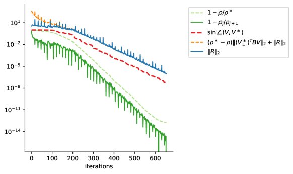
Figure 1: Numerical and theoretical quantities to check the convergence of the approximate solution to TR to the exact solution.

Figure 1 shows the values of $\sin(V,V^{\ast})$ in the iterations, along with the numerator of the tighter bound in (15), and the relative error in estimating $\rho^{\ast}$. In a usual context, these quantities would not be available; therefore, we also compare them with two computable quantities, which are the spectral norm of the residual matrix, and the relative difference between two consecutive trace ratio values.

We observe that the quantities depending solely on the trace ratio values decay faster than $\sin(V,V^{\ast})$, meaning that a stopping criterion based on this would give an unsatisfactory solution. The numerator in the bound (15) approaches $\|R\|_{2}$ in few iterations, suggesting that the norm of the residual is the dominant term. Both quantities follow $\sin(V,V^{\ast})$ with the same slope.

Motivated by the example, we further analyze the term $\rho^{\ast}-\rho$. We show that this quantity can be mostly explained by $\|R\|_{2}^{2}$. Let us decompose $V^{\ast}$ as $V^{\ast}=VE+V_{\perp}F$, and let $\beta^{\ast}=\mathop{{\rm tr}}((V^{\ast})^{T}BV^{\ast})$. Then

$$(\rho^{\ast}-\rho)\beta^{\ast}=\mathop{{\rm tr}}\Big{(}[E^{T}F^{T}]\begin{bmatrix}\Lambda&\bar{R}^{T}\\ \bar{R}&\bar{M}\end{bmatrix}\begin{bmatrix}E\\ F\end{bmatrix}\Big{)},$$

where $\bar{R}=V_{\perp}^{T}(A-\rho B)V$, $\bar{M}=V_{\perp}^{T}(A-\rho B)V_{\perp}$, and $\|\bar{R}\|_{2}=\|R\|_{2}$. Since $\mathop{{\rm tr}}(\Lambda)=\sum_{i=1}^{k}\lambda_{i}=0$ and from Courant–Fischer Theorem (see, e.g., [17]), one can quickly see that

$$0\leq\rho^{\ast}-\rho\leq\frac{\sum_{i=1}^{k}(\lambda_{i}(A-\rho B)-\lambda_{i})}{\sum_{i=1}^{k}\lambda_{p-k+i}(B)}.$$

Now let $\mu_{i}$ be the $i$th largest eigenvalue of the block diagonal matrix ${\rm diag}(\Lambda,\bar{M})$. [13, Cor. 1] shows that $|\lambda_{i}(A-\rho B)-\mu_{i}|\leq\delta^{-1}\|R\|^{2}_{2}$, where $\delta:=\min_{i,j}|\lambda_{i}(\Lambda)-\lambda_{j}(\bar{M})|$ measures the separation between the spectra of $\Lambda$ and $\bar{M}$. Then

$$\sum_{i=1}^{k}(\lambda_{i}(A-\rho B)-\lambda_{i}) \leq\sum_{i=1}^{k}(|\lambda_{i}-\mu_{i}|+|\lambda_{i}(A-\rho B)-\mu_{i}|)$$

$$\leq\sum_{i=1}^{k}|\lambda_{i}-\mu_{i}|+k\delta^{-1}\|R\|^{2}_{2}.$$

As remarked by Stewart in [25], there are bounds in the literature that do not depend on $\delta$, but they are linear in the residual norm. He states that the price one pays for the $\mathcal{O}(\|R\|^{2}_{2})$ bound is the dependence of the bound on a separation term.

We also observe that this bound does not depend on $(V^{\ast},\rho^{\ast})$. The open question remains whether we can determine a bound for $\sum_{i=1}^{k}|\mu_{i}-\lambda_{i}|$ in terms of $\|R\|_{2}$. Given the choices made for the expansion and the extraction phase, it is reasonable to expect that, as $\|R\|_{2}\to 0$, the eigenvalues of $\Lambda$ will coincide with the largest eigenvalues of ${\rm diag}(\Lambda,M)$. However, there might be some rare situations where $V$ fails to converge to the subspace spanned by the eigenvectors of $A-\rho^{\ast}B$, corresponding to the $k$ largest eigenvalues. The following example shows what we would observe in a typical case.

Example 11 (Continuation of Example 10).

The left plot of Figure 2 shows the behavior of $(\rho^{\ast}-\rho)\beta^{\ast}$. In this example, the squared norm of the residual seems to be an appropriate upper bound for this quantity. We also plot $\sum_{i=1}^{k}|\mu_{i}-\lambda_{i}|$, which drops after few iterations. At the same time, the eigenvalues of $H-\rho K$ approach the $k$ largest eigenvalues of $A-\rho B$. This can be seen in the right plot of Figure 2.

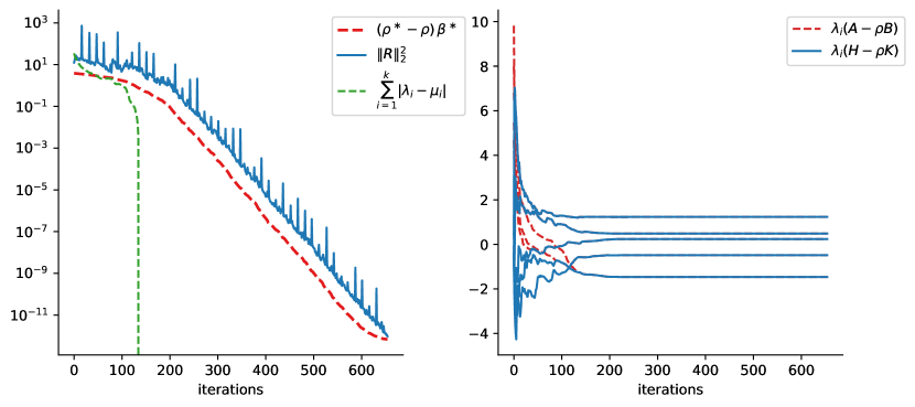
Figure 2: On the left: $(\rho^{\star}-\rho)\beta^{\ast}$ is bounded by the squared norm of the residual matrix. On the right: the approximate eigenvalues $\lambda_{i}(H-\rho K)$ converge to the $k$ largest eigenvalues of $A-\rho B$ throughout the iterations.

5 Classification task

We aim to compare the performance of Algorithm 1 with that of Algorithm 2, and FDA, in the context of classification problems. We provide a description of multigroup classification and introduce the relevant quantities involved in TR and FDA. In view of the numerical experiments of Section 6, some practical aspects are discussed, including the implementation of a subspace method for FDA.

Suppose we have a population described by the random vector $\mathbf{X}=(X_{1},\dots,X_{p})^{T}$, with mean $\mathbb{E}(\mathbf{X})=\boldsymbol{\mu}$ and covariance $\text{Var}(\mathbf{X})=\Sigma$. We make the common assumption that $\Sigma$ is nonsingular and so is its estimator. The population is divided into $g$ groups (or classes), modeled by the class variable $Y\in\{1,\dots,g\}$. Denote the expectation of $\mathbf{X}_{i}=(\mathbf{X}\mid Y=i)$ by $\mathbb{E}(\mathbf{X}_{i})=\boldsymbol{\mu}_{i}$, and its covariance matrix by $\text{Var}(\mathbf{X}_{i})=\Sigma_{i}$. The a priori probability of being in group $i$ is $p_{i}=P(Y=i)$.

Given a new observation $\mathbf{x}\in\mathbb{R}^{p}$, we would like to assign it to one of the $g$ classes, via a so-called classification rule, that is built on top of the available data. Let $\mathbf{x}_{i1},\dots,\mathbf{x}_{in_{i}}$ represent $n_{i}$ realizations of a random sample of $\mathbf{X}_{i}$; the total sample size is $n=\sum_{i=1}^{g}n_{i}$. We store the data row-wise, in an $n\times p$ matrix $X$. The sample mean and the sample covariance matrix of group $i$ are $\overline{\mathbf{x}}_{i}=n_{i}^{-1}\,\sum_{h=1}^{n_{i}}{\mathbf{x}_{ih}}$ and $S_{i}=n_{i}^{-1}\,\sum_{h=1}^{n_{i}}\,(\mathbf{x}_{ih}-\overline{\mathbf{x}}_{i})\,(\mathbf{x}_{ih}-\overline{\mathbf{x}}_{i})^{T}$, respectively. The overall sample mean is estimated by $\overline{\mathbf{x}}=\sum_{i=1}^{g}\tfrac{n_{i}}{n}\,\overline{\mathbf{x}}_{i}$. We define the classical between-class scatter matrix, $S_{B}$, and the classical within-class scatter matrix, $S_{W}$, as follows:

(16) $$S_{B}=n^{-1}\,\sum_{i=1}^{g}n_{i}\,(\overline{\mathbf{x}}_{i}-\overline{\mathbf{x}})\,(\overline{\mathbf{x}}_{i}-\overline{\mathbf{x}})^{T},\qquad S_{W}=n^{-1}\,\sum_{i=1}^{g}\sum_{h=1}^{n_{i}}\ (\mathbf{x}_{ih}-\overline{\mathbf{x}}_{i})\,(\mathbf{x}_{ih}-\overline{\mathbf{x}}_{i})^{T}.$$

From the definition of the overall mean and the group means, we deduce that ${\rm rank}(S_{B})\leq\min\{p,g-1\}$, while ${\rm rank}(S_{W})\leq\min\{p,n-g\}$. In both TR and FDA for multigroup classification, we look for a subspace that minimizes the distance within the projected groups while maximizing the distance between the projected groups. Therefore we set $A=S_{B}$ and $B=S_{W}$ in (1) for TR, and in (2) for FDA.

In subspace methods, it is sufficient to know how the scatter matrices act on a vector, without storing them. We make some practical considerations. First, the sum of the two scatter matrices gives the total sample covariance matrix, which represents the distance of each point from the center of the whole distribution:

(17) $$S_{T}=n^{-1}\,\sum_{i=1}^{g}\sum_{h=1}^{n_{i}}\,(\mathbf{x}_{ih}-\overline{\mathbf{x}})\,(\mathbf{x}_{ih}-\overline{\mathbf{x}})^{T}=S_{W}+S_{B}.$$

Simple computations also show that $S_{T}=n^{-1}X^{T}X-\overline{\mathbf{x}}\,\overline{\mathbf{x}}^{T}$. In addition, the covariance matrices (16) can be written as the product of the following matrices (see, e.g., [34]):

(18) $$H_{B} =[\sqrt{n_{1}}\,(\overline{\mathbf{x}}_{1}-\overline{\mathbf{x}}),\,\dots,\,\sqrt{n_{g}}\,(\overline{\mathbf{x}}_{g}-\overline{\mathbf{x}})]\in\mathbb{R}^{p\times g}$$

$$H_{W} =[\mathbf{x}_{ih}-\overline{\mathbf{x}}_{i}\mid i=1,\dots,g\ \text{and}\ h=1,\dots,n_{i}]\in\mathbb{R}^{p\times n}.$$

Then $S_{B}=H_{B}H_{B}^{T}$ and $S_{W}=H_{W}H_{W}^{T}$. In practice, we only use the decomposition of $S_{B}$, and compute $S_{W}=S_{T}-S_{B}$, which is more convenient. Then, apart from the data matrix, one would only need to store the group means and the overall mean to obtain the matrix-vector products $S_{B}\mathbf{v}$ and $S_{W}\mathbf{v}$, for $\mathbf{v}\in\mathbb{R}^{p}$. The second product is the most expensive and amounts to $\mathcal{O}(pn)$ operations; the first one requires $\mathcal{O}(gp)$ flops. However, we note that forming and storing $S_{W}$ costs $\mathcal{O}(p^{2}n)$, and therefore it might still be more convenient to compute $H_{W}(H_{W}^{T}\mathbf{v})$ at each iteration.

5.1 A Davidson type method for FDA

The trace ratio method is often compared to FDA in the context of multigroup classification. Therefore, we have implemented a Davidson type method to find the largest generalized eigenvalues of $(A,B)$ and their corresponding eigenvectors. This is described in Algorithm 3.

We remark that Davidson’s methods for the generalized eigenvalue problem can be found in the literature in, e.g., [14, 15, 19]. In [15], Davidson’s method is used for the computation of harmonic Ritz values. As for the basis of the search subspace, there are two possibilities: choosing a basis with orthonormal or $B$-orthogonal columns. The extraction phase changes accordingly. In the first case, we have to solve a projected generalized eigenvalue problem. In the second one, the $B$-orthogonal basis transforms the projected problem into a standard eigenvalue problem (see, e.g., [19, Alg. 2]). We prefer the first option, because it is generally favorable for the stability of the method, particularly for an ill-conditioned $B$. This choice is also suggested in [14, 15] and [19, Alg. 3]. Note that, with a search space spanned by orthonormal vectors, the approximate eigenvectors are automatically $B$-orthogonal.

Algorithm 3 A Davidson type method for FDA

Input: Symmetric $A\in\mathbb{R}^{p\times p}$, SPD $B\in\mathbb{R}^{p\times p}$, $k<p$, maximum and minimum dimensions with $k\leq{\sf m_{1}}<{\sf m_{2}}\leq p$, block size $1\leq{\sf m}\leq k$, initial $p\times{\sf m_{1}}$ matrix $U_{\sf m_{1}}$ with orthogonal columns, tolerance tol.
Output: $p\times k$ matrix $V$ with orthonormal columns maximizing the trace ratio.
1: Compute $AU_{\sf m_{1}}$, $BU_{\sf m_{1}}$ and $H_{\sf m_{1}}=U_{\sf m_{1}}^{T}\!AU_{\sf m_{1}}$, $K_{\sf m_{1}}=U_{\sf m_{1}}^{T}\!BU_{\sf m_{1}}$; $j={\sf m_{1}}$ 2: for $i=1,2,\dots$ 3:   M Solve GEP for $(H_{j},K_{j})$, store $k$ leading eigenvectors in $Z$, eigenvalues in $\Lambda$ 4:   M $V=U_{j}X$,  $R=AV-BV\Lambda=AU_{j}Z-BU_{j}Z\Lambda$ 5:   M Compute $U_{\sf m}=[\mathbf{u}_{j+1},\dots,\mathbf{u}_{j+{\sf m}}]$ largest left singular vectors of $R$ 6:   M if $\|R\|_{2}<{\sf tol}$,  return,  end 7:   M if $j={\sf m_{2}}$: 8:   MM Store ${\sf m_{1}}$ leading generalized eigenvectors of $(H_{\sf m_{2}},K_{\sf m_{2}})$ in $Z_{\sf m_{1}}=[Z\ Z_{{\sf m_{1}}-k}]$ 9:   MM Orthogonalize $Z_{\sf m_{1}}=Q_{\sf m_{1}}S_{\sf m_{1}}$ 10:   MM Set $j={\sf m_{1}}$, shrink $U_{j}=U_{\sf m_{2}}Q_{\sf m_{1}}$, $AU_{j}=AU_{\sf m_{2}}Q_{\sf m_{1}}$, $BU_{j}=BU_{\sf m_{2}}Q_{\sf m_{1}}$   MMm $H_{j}=Q_{\sf m_{1}}^{T}\!H_{\sf m_{2}}Q_{\sf m_{1}}$, $K_{j}=Q_{\sf m_{1}}^{T}\!K_{\sf m_{2}}Q_{\sf m_{1}}$ 11:   M end 12:   M Reorthogonalize $U_{\sf m}$ against $U_{j}$, expand $U_{j+1}=[U_{j}\ U_{\sf m}]$ 13:   M Compute $A\,U_{\sf m}$, $B\,U_{\sf m}$ and $U_{j+1}^{T}\!A\,U_{\sf m}$, $U_{j+1}^{T}\!B\,U_{\sf m}$ 14:   M $j=j+1$ 15: end

In the expansion phase, we maintain the choice made for TR, and use the $1\leq{\sf m}\leq k$ largest left singular vectors of the residual matrix. Reorthogonalization is also performed, as in Section 3.2.

The restarting procedure consists in using the ${\sf m_{1}}$ leading approximate generalized eigenvectors, extracted from the subspace $\mathcal{U}_{{\sf m_{2}}}$. This is similar to what has been done in [14], but also analogous to the restarting procedure in the Krylov–Schur method [29].

As in Section 3.3, we note that it is unnecessary to perform the extraction phase immediately after restarting, to get a new residual matrix. We start by recalling that the generalized eigenvalue problem for the first $k$ eigenvectors is also an optimization problem of the form (2). As in Proposition 4, if $\mathcal{U}_{{\sf m_{1}}}\subset\mathcal{U}_{{\sf m_{2}}}$, it holds

(19) $$\max_{V\,\subset\,\mathcal{U}_{{\sf m_{1}}},\,V^{T}BV=I_{k}}\mathop{{\rm tr}}(V^{T}\!AV)\leq\max_{V\,\subset\,\mathcal{U}_{{\sf m_{2}}},\,V^{T}BV=I_{k}}\mathop{{\rm tr}}(V^{T}\!AV).$$

We show that our restarting procedure attains equality in (19). Suppose the current search subspace is spanned by $U_{\sf m_{2}}\in\mathbb{R}^{p\times{\sf m_{2}}}$, and let $(H_{\sf m_{2}},K_{\sf m_{2}})$ be the corresponding projected $(A,B)$. Let $Z_{\sf m_{1}}=[Z\ Z_{{\sf m_{1}}-k}]$ contain the ${\sf m_{1}}$ largest generalized eigenvectors of $(H_{\sf m_{2}},K_{\sf m_{2}})$, where $Z$ is ${\sf m_{2}}\times k$, $Z_{{\sf m_{1}}-k}$ is ${\sf m_{2}}\times({\sf m_{1}}-k)$; consider its QR decomposition $Z_{\sf m_{1}}=Q_{\sf m_{1}}S_{\sf m_{1}}=Q_{\sf m_{1}}[S_{k}\ S_{{\sf m_{1}}-k}]$, where $Q_{\sf m_{1}}$ is ${\sf m_{2}}\times{\sf m_{1}}$ with orthonormal columns, $S_{\sf m_{1}}$ is ${\sf m_{1}}\times{\sf m_{1}}$ and upper triangular, and $S_{k}$ is the first ${\sf m_{1}}\times k$ block of $S_{\sf m_{1}}$. We define the new search subspace $\mathcal{U}_{\sf m_{1}}$ as the span of $U_{{\sf m_{1}}}:=U_{\sf m_{2}}Q_{\sf m_{1}}$, which has orthogonal columns.

The extraction phase for $U_{\sf m_{1}}$ is

(20) $$\max_{V\,\subset\,\mathcal{U}_{{\sf m_{1}}},\,V^{T}BV=I_{k}}\mathop{{\rm tr}}(V^{T}\!AV)=\max_{\begin{subarray}{c}V=U_{\sf m_{1}}C,\\ C^{T}U_{\sf m_{1}}^{T}BU_{\sf m_{1}}C=I_{k}\end{subarray}}\mathop{{\rm tr}}(C^{T}U_{{\sf m_{1}}}^{T}AU_{\sf m_{1}}C),$$

where

$$I_{k} =C^{T}U_{\sf m_{1}}^{T}BU_{\sf m_{1}}C=C^{T}Q_{\sf m_{1}}^{T}U_{\sf m_{2}}^{T}BU_{\sf m_{2}}Q_{\sf m_{1}}C$$

$$=C^{T}S_{\sf m_{1}}^{-T}Z_{\sf m_{1}}^{T}K_{\sf m_{2}}Z_{\sf m_{1}}S_{\sf m_{1}}^{-1}C=C^{T}S_{\sf m_{1}}^{-T}S_{\sf m_{1}}^{-1}C.$$

We have used the fact that $Q_{\sf m_{1}}=Z_{\sf m_{1}}S_{\sf m_{1}}^{-1}$, and $Z_{\sf m_{1}}$ has $K_{\sf m_{2}}$-orthogonal columns. In addition $Z_{\sf m_{1}}^{T}H_{\sf m_{2}}Z_{\sf m_{1}}=\Lambda_{\sf m_{1}}$, where $\Lambda_{\sf m_{1}}$ contains the first ${\sf m_{1}}$ generalized eigenvalues of $(H_{\sf m_{2}},K_{\sf m_{2}})$. Therefore we also obtain $C^{T}U_{{\sf m_{1}}}^{T}AU_{\sf m_{1}}C=C^{T}S_{\sf m_{1}}^{-T}\Lambda_{\sf m_{1}}S_{\sf m_{1}}^{-1}C$. This establishes the equivalence between (20) and

$$\max_{C^{T}C=I_{k}}\mathop{{\rm tr}}(C^{T}\Lambda_{\sf m_{1}}C),$$

whose maximizer is $C=[I_{k}\ 0]^{T}$. The maximum corresponds to the sum of the $k$ largest generalized eigenvalues of $(H_{\sf m_{2}},K_{\sf m_{2}})$. This means that $U_{\sf m_{1}}C$ achieves equality in (19). In addition, since $V=U_{{\sf m_{1}}}C=U_{\sf m_{2}}Q_{\sf m_{1}}S_{k}$, the residual matrix related to the new iteration can be computed by using the old quantities, without performing the extraction phase (20).

5.2 Regularization in the large-scale setting

It may happen that the within-scatter matrix is numerically singular. In view of Proposition 1, this might lead to an infinite trace ratio for TR, and to a so-called singular pencil for the GEP, which is known to be challenging to solve. One possible solution would be to cut out the nullspace of $S_{W}$ and solve either TR or FDA in the range of $S_{W}$. This has been done in, e.g., [17]. However, in the large-scale setting, performing a full eigenvalue decomposition to find the range of $S_{W}$ is undesirable (and possibly unfeasible). Therefore we choose the simpler idea of regularizing $S_{W}$ and consider the TR (FDA) for $(S_{B},(1-\alpha)S_{W}+\alpha I_{p})$, with $\alpha\in(0,1]$. This idea was originally proposed by [5] in the context of quadratic discriminant analysis.

It is easy to show that this problem is equivalent to TR (FDA) for $(S_{B},S_{W}+\frac{\alpha}{1-\alpha}I_{p})$, with $\frac{\alpha}{1-\alpha}\in[0,\infty)$. The latter formulation justifies the omission of the multiplicative factor $\mathop{{\rm tr}}(S_{W})/p$, which is present in [5, Eq. (18)]. There is no easy way of choosing the right amount of regularization. One may select $\alpha$ such that the subspace $V(\alpha)$ leads to the highest performance metric of interest in the classification task.

We note that a regularization of TR has already been proposed in [34], for high-dimensional problems, i.e., situations where the number of data points is much smaller than the dimension of the problem ($n\ll p$), and the data points are linearly independent. In this scenario, [34, Thm. 4.2] shows the equivalence between the solution to a regularized TR and a trace ratio method preceded by the QR decomposition of the data matrix $X$. In the high-dimensional setting, a QR step should be quite cheap, given that $n\ll p$, and leads to a smaller TR problem. In this case, QR combined with TR would be a better strategy than exploiting subspace methods.

5.3 Classification rule

TR and FDA are linear dimensionality reduction methods, i.e., they provide a subspace of a given dimension, which should maximize the separation between the groups in the data matrix. The quality of the solution is usually assessed on the capability of the model to correctly classify new observations, given the projected data.

In the experiments, we evaluate TR and FDA solutions in terms of classification accuracy, which is the proportion of data points that have been correctly classified. To do so, we adopt linear discriminant analysis (LDA, see, e.g., [7, Sec. 4.3]) as classification rule: first, we project the data onto the subspace spanned by either the solution to TR or FDA, indicated by $V$. Then we compute the projected group means and pooled covariance matrix, which is a multiple of the projected within-scatter matrix: $V^{T}S_{\rm pooled}V=\frac{n}{n-g}V^{T}S_{W}V$.

A new observation is first projected and then classified to the group with the closest projected centroid, based on the Mahalanobis distance and the number of samples in each group. In other words, if $\mathbf{x}$ is the new observation, then it is assigned to group $j$ if

$$j=\operatorname*{\arg\!\min}_{i}\|V^{T}(\mathbf{x}-\overline{\mathbf{x}}_{i})\|^{2}_{(V^{T}S_{\rm pooled}V)^{-1}}-2\log\tfrac{n_{i}}{n}.$$

We acknowledge that, following the linear dimensionality reduction step, other classifiers could be chosen for assigning the new observations. However, a deeper study on this matter is out of the scope of the paper.

6 Experiments

We now compare the two versions of TR (cf. Algorithm 1 and Algorithm 2) and the subspace method for FDA (cf. Algorithm 3). The methods are evaluated in terms of number of matrix-vector (MV) products and computational time (in seconds). The quality of their solution is assessed in terms of classification accuracy, by implementing the classification rule in Section 5.3. As Algorithm 1 and Algorithm 2 yield approximately the same solution, the comparison of their accuracy acts mainly as a sanity check.

We run some experiments first on synthetic data and then on real datasets. We consider only situations where $n\gg p$, for the reasons remarked at the end of Section 5.2. Unless otherwise specified, we assume that the block size is ${\sf m}=1$.

6.1 Synthetic data

We consider the example from [18], with $g$ groups, $g$ relevant features, and $q>0$ other irrelevant variables. The input variables of the $i$th class are $\mathbf{X}_{i}\sim\mathcal{N}_{g+q}(2\mathbf{e}_{i},\Sigma)$, for $i=1,\dots,g$, where $\mathbf{e}_{i}$ is the $i$th vector of the canonical basis of $\mathbb{R}^{g+q}$, and the covariance matrix is

$$\Sigma=\begin{bmatrix}1&0.1&\cdots&0.1&\\ 0.1&1&0.1&\vdots&\\ 0.1&0.1&\ddots&0.1&\\ 0.1&\cdots&0.1&1&\\ &&&&I_{q}\end{bmatrix}$$

for all groups. In other words, $\Sigma$ is a block diagonal matrix, where the first $g\times g$ block has ones on the main diagonal, and 0.1 as off-diagonal elements. The second block is a $q\times q$ identity matrix. The remaining elements are zeros. In our experiments, we use $g=3$ groups, $q=5000$ irrelevant variables, $n_{i}=50000$ training data points per group, and $n_{i}=1000$ test data points per group. We run $50$ random experiments, where $(S_{B},S_{W})$ are estimated in the classical way, according to (16), using the training data. In both TR and FDA, we project the data on a subspace of dimension $k=2$. TR in Algorithm 1 is indicated as TR KSchur, given that the eigenvalues in the inner iterations are computed with the Krylov–Schur method. Davidson’s methods for TR and FDA are indicated as TR subspace and FDA subspace, respectively. In all methods, the algorithms stop when $10^{5}$ (outer) iterations are reached. The stopping criterion is based on the spectral norm of the residual (see Section 3.2): $\|R\|_{2}<{\sf tol}$, with ${\sf tol}=10^{-6}$. For the Krylov–Schur method, TR subspace and FDA subspace, the minimum size of the search subspace is ${\sf m_{1}}=2k=4$, the maximum size is ${\sf m_{2}}=4k=8$.

In this first experiment, we also test two different ways of performing the matrix-vector multiplication by the within covariance matrix. While the product with $S_{B}$ is always computed via the decomposition (18), in one case, we precompute and store $S_{W}$ (16), and perform simple matrix-vector products. Alternatively, we exploit the relations (17) and (18) to decompose both $S_{B}$ and $S_{W}$, with very little extra storage. For a fair comparison of the two techniques, the computational time for precomputing the scatter matrices is also taken into account.

Table 1 shows the result of the simulations. All methods converge within $10^{5}$ iterations in all experiments. In this example, all methods give the same accuracy, even if, in general, TR and FDA provide different solutions. In particular, while the projection matrix of TR has orthonormal columns, the columns of the FDA solution are $S_{W}$-orthogonal.

In this example, FDA subspace and TR subspace show very similar performances, in terms of both average matrix-vector products and average computational time. TR KSchur requires more matrix-vector products and computational time. Because of this, the method benefits from the precomputation of the within covariance matrix. On the other hand, when fewer matrix-vector products are required (i.e., in TR subspace and FDA subspace), it is more convenient to compute the matrix-vector products by decomposing the scatter matrices.

Table 1: Results for the synthetic data, over $50$ experiments. Average (Avg) and standard deviation (Sd) of matrix-vector (MV) products, time (in seconds, $s$), and accuracy are reported. We also indicate whether the covariance matrices were precomputed and stored, or not.

Precomputed	$k$	Method	MV		Time ($s$)		Accuracy
			Avg	Sd	Avg	Sd	Avg	Sd
No	2	FDA subspace	22	0	9.0	0.1	0.85	$<0.01$
No	2	TR KSchur	70	0	27.5	0.1	0.85	$<0.01$
No	2	TR subspace	25	0.1	10.0	0.1	0.85	$<0.01$
Yes	2	FDA subspace	22	0	14.5	0.7	0.85	$<0.01$
Yes	2	TR KSchur	70	0	14.8	0.7	0.85	$<0.01$
Yes	2	TR subspace	25	0.1	14.6	0.7	0.85	$<0.01$

6.2 Real datasets

In what follows, we consider two real datasets to highlight problem-dependent behaviors of TR subspace, TR KSchur, and FDA subspace. In particular, we observe the algorithms for different levels of regularization $\alpha$ and reduced dimension $k$.

Fashion MNIST [32]

The dataset consists of $n=60000$ gray-scale images of fashion articles, with $p=784$ pixels. The pixels have been scaled by $255$, so each feature ranges in $[0,1]$. The number of classes is $g=10$. All classes are equally represented. We want to project the data onto a subspace of size $k=9$ and then classify the items with the LDA classifier. The classification accuracy is assessed via a 10-fold cross-validation. We run TR subspace, FDA subspace, and TR KSchur. For the three methods, the size of the search subspace varies between ${\sf m_{1}}=2k=18$ and ${\sf m_{2}}=5k=45$. Here we show how regularization affects the various methods, by setting $\alpha=0$ (i.e., no regularization) and $\alpha=0.1$. Results are shown in Table 2.

Table 2: Results of the 10-fold cross-validation on Fashion MNIST. Average (Avg) and standard deviation (Sd) of matrix-vector (MV) products, time (in seconds, $s$), and accuracy are reported. Different levels of regularization $\alpha$ are considered.

$\alpha$	$k$	Method	MV		Time ($s$)		Accuracy
			Avg	Sd	Avg	Sd	Avg	Sd
0	9	FDA subspace	17095	2606	9.4	2.6	0.82	$<0.01$
0	9	TR KSchur	79231	3995	7.8	0.5	0.48	0.01
0	9	TR subspace	9004	262	5.9	1.2	0.48	0.01
0.1	9	FDA subspace	163	1	0.5	$<0.01$	0.80	$<0.01$
0.1	9	TR KSchur	34807	1529	3.7	0.2	0.59	$<0.01$
0.1	9	TR subspace	7095	370	4.3	0.2	0.59	$<0.01$

First we note that TR subspace requires fewer matrix-vector products compared to TR KSchur, but it is less competitive in terms of computational time when $\alpha=0.1$. All three algorithms benefit from the regularization of $S_{W}$. This holds especially for FDA subspace. Regularization also improves the accuracy of the TR problem, from $48\%$ to $59\%$.

We now compare the behavior of TR KSchur, TR subspace, and FDA subspace throughout the iterations. We consider one of the splits in the 10-fold cross-validation, and plot the number of matrix-vector products per iteration against the spectral norm of the residual matrix, which constitutes the stopping criterion. We also run the two subspace methods without restart, which corresponds to setting ${\sf m_{2}}=p=784$. The idea is to check how well the restarting procedure behaves.

Results are shown in Figure 3. As already suggested by Table 2, the behavior of FDA changes significantly when regularization is added, for both ${\sf m_{2}}=5k$ and ${\sf m_{2}}=p$. The method does not show as many oscillations in $\|R\|_{2}$ as in the case $\alpha=0$. A possible hint for the slow convergence might be found in the fact that, before regularization, $\lambda_{p}(S_{W})\approx 10^{-7}$. When $\alpha=0.1$, $\lambda_{p}((1-\alpha)S_{W}+\alpha I_{p})\approx 10^{-2}$. An advantage of this regularization is that an $S_{W}$ with a larger minimal singular value avoids the problematic occurrence of almost singular pencils. Regularization seems to have a smaller impact on the behavior of TR subspace and TR KSchur. In particular, TR subspace with restart shows many oscillations in both cases. TR KSchur behaves differently since it performs fewer outer iterations, that require several inner matrix-vector products. As we have already observed, it converges in more matrix-vector products than TR subspace.

Figure 4 shows the value of the trace ratio per number of matrix-vector products. Interestingly, TR subspace gets close to the optimal trace ratio value faster than TR KSchur.

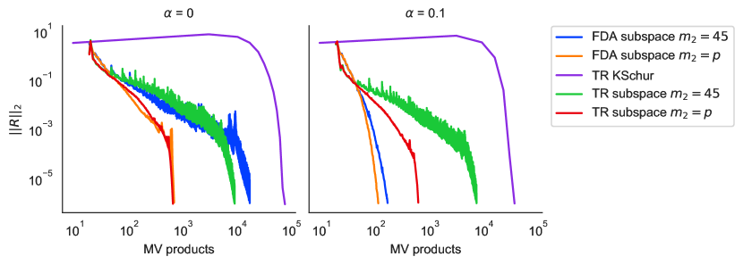
Figure 3: FDA and TR for Fashion MNIST, solved by various methods. The number of matrix-vector (MV) products is plotted against the spectral norm of the residual matrix, $\|R\|_{2}$. The graphs are for different levels of regularization in $S_{W}$.

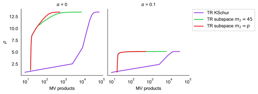
Figure 4: Trace ratio value $\rho$ per number of matrix-vector (MV) products. The graphs are for different levels of regularization in $S_{W}$.

German Traffic Sign Recognition [23]

The second dataset consists of $n=39209$ traffic signs, described by $p=6052$ features (HOG features, see [23] for more details), and divided into $g=43$ classes. The dataset is unbalanced, with $n_{i}\in[270,3000]$. The classification accuracy is assessed via a 10-fold cross-validation, with the LDA classifier. We run TR subspace, FDA subspace, and TR KSchur. For the three methods, the size of the search subspace is between ${\sf m_{1}}=2k$ and ${\sf m_{2}}=5k$. Given the large number of classes, we consider several reduced dimensions $k\in\{10,20,30\}$. We also test the block versions of the methods, with block size ${\sf m}=5$ (cf. [35] for a block Krylov–Schur method). In this example, the regularization parameter is set to $\alpha=0.1$.

The results of the 10-fold cross-validation are shown in Table 3. First we notice that, for all $k$, FDA gives slightly better results in terms of accuracy. Increasing $k$ leads to an increase of the average number of matrix-vector products (and computational time) for all methods. TR subspace and FDA subspace methods with block size ${\sf m}=5$ are on average faster than their counterparts with ${\sf m}=1$ in terms of computational time; nevertheless TR subspace with ${\sf m}=5$ tends to require more matrix-vector products than TR subspace with ${\sf m}=1$. TR KSchur with ${\sf m}=5$ seems to be slower than TR KSchur with ${\sf m}=1$, and shows a larger variability compared to the other methods. Among the TR methods, TR subspace with ${\sf m}=1$ is the one that requires the smallest average number of matrix-vector products for convergence; TR subspace with ${\sf m}=5$ is the least expensive in terms of computational time.

Table 3: Results of the 10-fold cross-validation on German Traffic Sign Recognition. Average (Avg) and standard deviation (Sd) of matrix-vector (MV) products, time (in seconds, $s$), and accuracy are reported. Different reduced dimensions $k$ are considered. The regularization parameter is set to $\alpha=0.1$.

$k$	Method	MV		Time ($s$)		Accuracy
		Avg	Sd	Avg	Sd	Avg	Sd
10	FDA subspace	225	2	14.0	0.3	0.83	0.01
10	FDA subspace, ${\sf m}=5$	229	2	11.8	0.3	0.83	0.01
10	TR KSchur	1022	15	21.4	0.4	0.74	0.01
10	TR Kschur, ${\sf m}=5$	9413	2788	35.5	7.3	0.74	0.01
10	TR subspace	574	9	19.1	0.3	0.74	0.01
10	TR subspace, ${\sf m}=5$	1175	100	15.4	0.5	0.74	0.01
20	FDA subspace	338	1	16.9	0.3	0.93	0.01
20	FDA subspace, ${\sf m}=5$	340	0	12.4	0.3	0.93	0.01
20	TR KSchur	2524	99	39.4	1.0	0.92	$<0.01$
20	TR Kschur, ${\sf m}=5$	8810	1797	35.2	4.9	0.92	$<0.01$
20	TR subspace	1683	32	43.4	0.6	0.92	$<0.01$
20	TR subspace, ${\sf m}=5$	2982	183	24.4	0.7	0.92	$<0.01$
30	FDA subspace	419	1	20.3	0.3	0.95	$<0.01$
30	FDA subspace, ${\sf m}=5$	420	0	13.1	0.3	0.95	$<0.01$
30	TR KSchur	6936	360	96.9	4.9	0.94	$<0.01$
30	TR Kschur, ${\sf m}=5$	36297	3370	115.9	10.0	0.94	$<0.01$
30	TR subspace	4553	118	130.5	3.7	0.94	$<0.01$
30	TR subspace, ${\sf m}=5$	11206	979	77.4	6.2	0.94	$<0.01$

In this problem, the slow convergence of TR is probably due to the fact that there is a small gap between the $k$th and the $(k+1)$st largest eigenvalues of the matrix $S_{B}-\rho^{\ast}S_{W}$ (cf. the discussion in Section 2). The gap decreases as the reduced dimension increases. For instance, for one of the $10$ splits we observe the following: for $k=10$, the gap is $\lambda_{k+1}-\lambda_{k}\approx 10^{-3}$, for $k=20$ it is $\lambda_{k+1}-\lambda_{k}\approx 10^{-4}$, for $k=30$, it is of order $10^{-6}$.

We note that, when the gap is numerically zero and uniqueness is lost, there is no guarantee that different solutions will provide the same classification results. Therefore, one might consider monitoring $\lambda_{k}(U^{T}(A-\rho B)U)-\lambda_{k+1}(U^{T}(A-\rho B)U)$ as an approximate value for $\lambda_{k}(A-\rho^{\ast}B)-\lambda_{k+1}(A-\rho^{\ast}B)$, where $U$ is the output search subspace of Algorithm 2. If this gap is not satisfactory, the user may decide to choose a different reduced dimension to run TR.

7 Conclusions

We have introduced a Davidson type subspace method for large-scale trace ratio problems. The details about the algorithm are covered in Section 3. In the extraction phase, a projected trace ratio problem is solved through the conventional Newton type routine for TR, as outlined in Algorithm 1. The information gathered within the residual matrix has been used to expand the search subspace. We have also designed a restart strategy to maintain a non-decreasing trace ratio value throughout the iterations.

Section 4 analyzes the behavior of the approximate solution to TR. As the angle between the search subspace and the solution to TR approaches zero, there is a subset of approximate eigenvalues approaching the largest eigenvalues of $A-\rho^{\ast}B$. This stems from the trace ratio value converging towards $\rho^{\ast}$ as the accuracy of the search subspace improves. If the largest eigenvalues of $A-\rho^{\ast}B$ are uniformly separated from some unwanted approximate eigenvalues, the angle between the approximate solution and the solution to TR also approaches zero.

Additionally, we have shown that this angle is bounded by the spectral norm of the residual matrix, augmented by a term that depends on the gap between $\rho^{\ast}$ and the current approximate trace ratio value. In typical situations, we expect this quantity to be bounded quadratically by the norm of the residual matrix. To some extent, this fact justifies the use of the spectral norm of the residual matrix in the computation of the stopping criterion.

The trace ratio problem finds common application in multigroup classification, which we have revisited in Section 5. Additionally, we have also presented an implementation of a Davidson type method for FDA, offering more insights into its restart mechanism.

Section 6 presents a numerical analysis of subspace methods for both the trace ratio problem (TR subspace) and FDA (FDA subspace), along with the Newton-type algorithm for TR (TR KSchur). This comparison involves both synthetic and real datasets. It seems that TR subspace requires fewer matrix-vector products than TR KSchur to converge to the TR maximizer. The difference is even more pronounced in the convergence of the trace ratio value towards $\rho^{\ast}$. In the context of real datasets, and in contrast to FDA subspace, the norm of the residual matrix exhibits more oscillations in TR subspace. This may be partly caused by a relatively narrow gap between the $k$th and $(k+1)$st eigenvalues of $A-\rho^{\ast}B$. While the regularization technique discussed in Section 5.2 has proven effective in improving the convergence speed of FDA, finding an appropriate regularization strategy for TR might be challenging, as the width of the gap itself depends on the optimal trace ratio value.

An implementation of TR KSchur, TR subspace, and FDA subspace is available in Matlab at github.com/gferrandi/traceratio-matlab.

Acknowledgments: This work is supported by the European Unions Horizon 2020 programme under the Marie Sklodowska-Curie Grant Agreement no. 812912. It has also received support from Fundação para a Ciência e Tecnologia, Portugal, through the project UIDB/04621/2020, with DOI 10.54499/UIDB/04621/2020.

References

- [1] P. A. Absil, R. Mahony, and R. Sepulchre. Optimization Algorithms on Matrix Manifolds. Princeton University Press, Princeton, NJ, USA, 2009.
- [2] M. Crouzeix, B. Philippe, and M. Sadkane. The Davidson method. SIAM J. Sci. Comput., 15(1):62–76, 1994.
- [3] A. Edelman, T. A. Arias, and S. T. Smith. The geometry of algorithms with orthogonality constraints. SIAM J. Matrix Anal. Appl., 20(2):303–353, 1998.
- [4] G. Ferrandi, I. V. Kravchenko, M. E. Hochstenbach, and M. R. Oliveira. On the trace ratio method and Fisher’s discriminant analysis for robust multigroup classification. preprint arXiv:2211.08120, 2022.
- [5] J.H. Friedman. Regularized discriminant analysis. J. Am. Stat. Assoc., 84(405):165–175, 1989.
- [6] Y. F. Guo, S. J. Li, J. Y. Yang, T. T. Shu, and L. D. Wu. A generalized Foley–Sammon transform based on generalized Fisher discriminant criterion and its application to face recognition. Pattern Recognit. Lett., 24(1-3):147–158, 2003.
- [7] T. Hastie, R. Tibshirani, and J. Friedman. The Elements of Statistical Learning. Springer Series in Statistics. Springer New York Inc., New York, NY, USA, 2009.
- [8] Z. Jia and F. Lai. A convergence analysis on the iterative trace ratio algorithm and its refinements. CSIAM Trans. Appl. Math., 2(2):297–312, 2021.
- [9] Z. Jia and G. W. Stewart. An analysis of the Rayleigh–Ritz method for approximating eigenspaces. Math. Comput., 70(234):637–647, 2000.
- [10] R.A. Johnson and D.W. Wichern. Applied Multivariate Statistical Analysis. Prentice Hall, Upper Saddle River, NJ, USA, 6th edition, 2007.
- [11] A. V. Knyazev. Toward the optimal preconditioned eigensolver: Locally optimal block preconditioned conjugate gradient method. SIAM J. Sci. Comp, 23(2):517–541, 2001.
- [12] A.V. Knyazev and M.E. Argentati. Principal angles between subspaces in an A-based scalar product: algorithms and perturbation estimates. SIAM J. Sci. Comp., 23(6):2008–2040, 2002.
- [13] R. Mathias. Quadratic residual bounds for the Hermitian eigenvalue problem. SIAM J. Matrix Anal. Appl., 19(2):541–550, 1998.
- [14] R. B. Morgan. Davidson’s method and preconditioning for generalized eigenvalue problems. J. Comput. Phys., 89(1):241–245, 1990.
- [15] R. B. Morgan. Computing interior eigenvalues of large matrices. Linear Algebra Appl., 154:289–309, 1991.
- [16] R. B. Morgan and D. S. Scott. Generalizations of Davidson’s method for computing eigenvalues of sparse symmetric matrices. SIAM J. Sci. Stat. Comput., 7(3):817–825, 1986.
- [17] T. T. Ngo, M. Bellalij, and Y. Saad. The trace ratio optimization problem. SIAM Rev., 54(3):545–569, 2012.
- [18] I. Ortner, P. Filzmoser, and C. Croux. Robust and sparse multigroup classification by the optimal scoring approach. Data Min. Knowl. Discov., 34(3):723–741, 2020.
- [19] E. Romero and J. E. Roman. A parallel implementation of davidson methods for large-scale eigenvalue problems in SLEPc. ACM Trans. Math. Softw., 40(2):1–29, 2014.
- [20] Y. Saad. Numerical Methods for Large Eigenvalue Problems. SIAM, Philadelphia, PA, 2011.
- [21] H. Shen, K. Diepold, and K. Hüper. A geometric revisit to the trace quotient problem. In MTNS 2010, pages 1–7, 2010.
- [22] G. L. G. Sleijpen and H. A. Van der Vorst. A Jacobi–Davidson iteration method for linear eigenvalue problems. SIAM Rev., 42(2):267–293, 2000.
- [23] J. Stallkamp, M. Schlipsing, J. Salmen, and C. Igel. The German traffic sign recognition benchmark: a multi-class classification competition. In Proc. Int. Jt. Conf. Neural Netw., pages 1453–1460. IEEE, 2011.
- [24] A. Stathopoulos, Y. Saad, and K. Wu. Dynamic thick restarting of the Davidson, and the implicitly restarted Arnoldi methods. SIAM J. Sci. Comput., 19(1):227–245, 1998.
- [25] G. W. Stewart. Error and perturbation bounds for subspaces associated with certain eigenvalue problems. SIAM Rev., 15(4):727–764, 1973.
- [26] G. W. Stewart. A generalization of Saad’s theorem on Rayleigh–Ritz approximations. Linear Algebra Appl., 327(1-3):115–119, 2001.
- [27] G. W. Stewart. Matrix Algorithms. Vol. II. SIAM, Philadelphia, PA, 2001.
- [28] G. W. Stewart and J. G. Sun. Matrix Perturbation Theory. Academic Press Inc., Boston, MA, 1990.
- [29] G.W. Stewart. A Krylov–Schur algorithm for large eigenproblems. SIAM J. Matrix Anal. Appl., 23(3):601–614, 2002.
- [30] H. Wang, S. Yan, D. Xu, and X. Huang. Trace-ratio vs. ratio-trace for dimensionality reduction. Proc. IEEE Comput. Soc. Conf. Comput. Vis. Pattern Recognit., pages 1–8, 2007.
- [31] K. Wu and H. Simon. Thick-restart Lanczos method for large symmetric eigenvalue problems. SIAM J. Matrix Anal. Appl., 22(2):602–616, 2000.
- [32] H. Xiao, K. Rasul, and R. Vollgraf. Fashion-MNIST: a novel image dataset for benchmarking machine learning algorithms. preprint arXiv:1708.07747, 2017.
- [33] L. H. Zhang and R. C. Li. Maximization of the sum of the trace ratio on the stiefel manifold, ii: Computation. Sci. China Math., 58(7):1549–1566, 2015.
- [34] L. H. Zhang, L. Z. Liao, and M. K. Ng. Fast algorithms for the generalized Foley–Sammon discriminant analysis. SIAM J. Matrix Anal. Appl., 31(4):1584–1605, 2010.
- [35] Y. Zhou and Y. Saad. Block Krylov–Schur method for large symmetric eigenvalue problems. Numer. Algorithms, 47:341–359, 2008.