Attractors in STGR with Boundary Correction

Abstract

We investigate the asymptotic behavior of the cosmological field equations in Symmetric Teleparallel General Relativity, where a nonlinear function of the boundary term is introduced instead of the cosmological constant to describe the acceleration phase of the universe. Our analysis reveals constraints on the free parameters necessary for the existence of an attractor that accurately represents acceleration. However, we also identify asymptotic solutions depicting Big Rip and Big Crunch singularities. To avoid these solutions, we must impose constraints on the phase-space, requiring specific initial conditions.

I Introduction

Recent cosmological observations od1 ; od2 ; od3 challenge Einstein’s General Relativity (GR). In recent years, many cosmologists have proposed various modified gravitational models to explain these observations Buda ; Ferraro ; mod1 ; rt11 ; rt12 ; f6 ; rt1 ; rt2 ; rt4 ; rt5 ; rt7 ; rt10 ; ff3 ; ff4 ; ff5 ; rr5 ; rr6 . Although these models can be examined using numerical techniques, analytical treatment is necessary to derive constraints on the models’ free parameters and draw conclusions about their cosmological viability.

In gravitational physics, the field equations are nonlinear differential equations, making the derivation of analytic solutions a challenging task. Certain approaches employed in the literature for constructing analytic solutions rely on symmetry analysis ns1 ; ns2 ; ns3 ; ns4 and the Painlevé algorithm p1 ; p2 ; p3 . However, in order to understand the global behaviour of the physical properties in a given gravitational model, we can study the behaviour of the field equations in the long run. The analysis of the asymptotics has been widely used in gravitational theories, yielding many interesting results dn1 ; dn2 ; dn3 ; dn4 ; dn5 ; dn6 ; dn7 ; dn8 ; dn9 ; dn10 .

In this work, we investigate the impact of nonlinear boundary corrections in Symmetric Teleparallel General Relativity (STGR) nester on cosmological solutions. In particular we assume the gravitational Lagrangian to be $L=Q+f\left(B\right)$, where $Q$ is the nonmetricity scalar, which is the fundamental scalar of STGR, and $f\left(B\right)$ is an arbitrary function of the boundary term $B$ which gives the difference of $Q$ with the Ricci scalar of the background spacetime. This model belongs to the the family of $f(Q,B)$-gravity, which proposed recently in ftc0 ; ftc1 ; ftc2 and it is a generalization of $f\left(Q\right)$ theory lav2 ; lav3 . The boundary term has been introduced before in the gravitational Action Integral previously within the framework of teleparallelism bah with various applications in cosmological studies, see for instance ftb1 ; ftb2 ; ftb3 ; ftb4 ; ftb5 .

The boundary term introduces higher-order derivatives into the field equations, which can be attributed to scalar fields anbound . These newly introduced scalar fields play a role in the field equations, imparting dynamic behavior to dark energy. In the following sections, we utilize asymptotic analysis to establish constraints on the free parameters of the gravitational theory and discuss the model’s viability based on initial conditions dn9 ; dn10 . The paper is structured as follows.

In Section II we briefly discuss the basic definitions of STGR and we introduce the boundary correction term. We consider a Friedmann–Lemaître–Robertson–Walker (FLRW) geometry and in Section III we present the field equations for the gravitational model of our consideration. Section IV includes the main results of this study where we present a detailed analysis of the dynamics for the cosmological field equations. Finally, in Section V we summarize our results.

II Symmetric Teleparallel General Relativity

Consider a four-dimensional (non-Riemannian) manifold characterized by the metric tensor $g_{\mu\nu}$ and the symmetric and flat connection $\Gamma_{\mu\nu}^{\kappa}$, defining the covariant derivative $\nabla_{\mu}$. Furthermore, we assume that the metric tensor and the connection $\Gamma_{\mu\nu}^{\kappa}$ possess identical symmetries.

Because $\Gamma_{\mu\nu}^{\kappa}$ differs from the Levi-Civita connection it follows $\nabla_{\lambda}g_{\mu\nu}\neq 0$. The tensor field

$$Q_{\lambda\mu\nu}\equiv\nabla_{\lambda}g_{\mu\nu}=\frac{\partial g_{\mu\nu}}{\partial x^{\lambda}}-\Gamma_{\;\lambda\mu}^{\sigma}g_{\sigma\nu}-\Gamma_{\;\lambda\nu}^{\sigma}g_{\mu\sigma}$$

is called the nonmetricity tensor and it is the essential for the STGR.

By definition, the connection is symmetric and flat, implying that both the curvature tensor and the torsion tensor vanish.

From the nonmetricity tensor we can construct the scalar $Q$ as nester

$$Q=Q_{\lambda\mu\nu}P^{\lambda\mu\nu},$$ (1)

which is the Lagrangian function of STGR.

In particular, in STGR the Action Integral is defined as

$$S_{STGR}=\int d^{4}x\sqrt{-g}Q.$$ (2)

Tensor $\ P^{\lambda\mu\nu}$ is given by the following expression nester

$$P_{\;\mu\nu}^{\lambda}=-\frac{1}{4}Q_{\;\mu\nu}^{\lambda}+\frac{1}{2}Q_{(\mu\phantom{\lambda}\nu)}^{\phantom{(\mu}\lambda\phantom{\nu)}}+\frac{1}{4}\left(Q^{\lambda}-\bar{Q}^{\lambda}\right)g_{\mu\nu}-\frac{1}{4}\delta_{\;(\mu}^{\lambda}Q_{\nu)},$$ (3)

and

$$Q_{\mu}=Q_{\mu\nu}^{\phantom{\mu\nu}\nu}~{},~{}\bar{Q}_{\mu}=Q_{\phantom{\nu}\mu\nu}^{\nu\phantom{\mu}\phantom{\mu}}.$$ (4)

Let $\tilde{\Gamma}_{\mu\nu}^{\kappa}$ be the Levi-Civita connection for the metric tensor $g_{\mu\nu}$, that is $\tilde{\nabla}_{\lambda}g_{\mu\nu}=0$, and $\tilde{R}$ is the Ricciscalar defined by the Levi-Civita connection. Then by definition lav3 $R-Q=B_{Q}$where $B$ is a boundary given by the expression lav3 $B_{Q}=-\tilde{\nabla}_{\mu}\left(Q^{\mu}-\bar{Q}^{\mu}\right)$.

Consequently it follows

$$\int d^{4}x\sqrt{-g}Q\simeq\int d^{4}x\sqrt{-g}R+\text{boundary terms.}$$ (5)

and the theory is equivalent to GR.

II.1 Boundary corrections

The influence of the boundary term on gravitational phenomena has been previously investigated, particularly in the context of teleparallel gravity bah .

In this study we consider the modified gravitational Action Integral

$$\hat{S}_{STGR}=\int d^{4}x\sqrt{-g}\left(Q+f\left(B\right)\right),$$ (6)

where we introduce a nonlinear function $f$ which depend on the boundary $B$. Action $\hat{S}_{STGR}$ belongs to the family of $f(Q,B)$ (also known as $f\left(Q,C\right)$) theory ftc0 ; ftc1 ; ftc2 . In our consideration we assume the dynamical degrees of freedom provided by the correction term $f\left(B\right)$ to play the role of a dynamical dark energy.

The gravitational field equations are

$$0 =\frac{2}{\sqrt{-g}}\nabla_{\lambda}\left(\sqrt{-g}P_{\;\mu\nu}^{\lambda}\right)-\frac{1}{2}\left(Q+B\right)g_{\mu\nu}+\left(P_{\mu\rho\sigma}Q_{\nu}^{\;\rho\sigma}-2Q_{\rho\sigma\mu}P_{\phantom{\rho\sigma}\nu}^{\rho\sigma}\right)$$

$$+\left(\frac{B}{2}g_{\mu\nu}-\nabla_{\mu}\nabla_{\nu}+g_{\mu\nu}g^{\kappa\lambda}\nabla_{\kappa}\nabla_{\lambda}-2P_{~{}~{}\mu\nu}^{\lambda}\nabla_{\lambda}\right)f_{,B},$$ (7)

or equivalent

$$G_{\mu\nu}=T_{\mu\nu}^{f\left(B\right)},$$ (8)

where now $G_{\mu\nu}$ is the Einstein tensor and $T_{\mu\nu}^{f\left(B\right)}$ attributes the dynamical degrees of freedom of the boundary term, that is,

$$T_{\mu\nu}^{f\left(B\right)}=\left(\nabla_{\mu}\nabla_{\nu}-g_{\mu\nu}g^{\kappa\lambda}\nabla_{\kappa}\nabla_{\lambda}+2P_{~{}~{}\mu\nu}^{\lambda}\nabla_{\lambda}\right)f_{,B}+\frac{1}{2}\left(f\left(B\right)-Bf_{,B}\right)g_{\mu\nu}.$$ (9)

We introduce the scalar field $\zeta=f_{,B}$; thus, the energy momentum tensor $T_{\mu\nu}^{f\left(B\right)}$ becomes

$$T_{\mu\nu}^{f\left(B\right)}=\left(\nabla_{\mu}\nabla_{\nu}\zeta-g_{\mu\nu}g^{\kappa\lambda}\nabla_{\kappa}\nabla_{\lambda}\zeta+2P_{~{}~{}\mu\nu}^{\lambda}\nabla_{\lambda}\zeta\right)+\frac{1}{2}V\left(\zeta\right)g_{\mu\nu},$$ (10)

where $V\left(\zeta\right)=\left(f\left(B\right)-Bf_{,B}\right).$

III FLRW Cosmology

On very large scales, the universe is isotropic and homogeneous, described by the spatially flat FLRW geometry with the line element

$$ds^{2}=-N\left(t\right)dt^{2}+a^{2}\left(t\right)\left(dx^{2}+dy^{2}+dz^{2}\right),$$ (11)

where $a\left(t\right)$ is the scale factor and $H\left(t\right)=\frac{1}{N}\frac{\dot{a}}{a}$ is the Hubble function and $N\left(t\right)$ is the lapse function, where without loss of generality we assume $N\left(t\right)=1$.

The FLRW geometry admits six isometries consisted by the three translation symmetries

$$\partial_{x}~{},~{}\partial_{y}~{},~{}\partial_{z}~{},$$

and the three rotations

$$y\partial_{x}-x\partial_{y}~{},~{}z\partial_{x}-x\partial_{z}~{},~{}z\partial_{y}-y\partial_{z}\text{.}$$

The requirement for the connection $\Gamma_{\mu\nu}^{\kappa}$ to be symmetric, flat, and to inherit the symmetries of the background geometry leads to three distinct families of connections Heis2 ; Zhao . The cosmological field equations for these three families of connections were derived previously in anbound .

For the first connection, namely $\Gamma_{1}$, the modified Friedmann equations are

$$-3H^{2} =3\dot{\zeta}H+\frac{1}{2}V\left(\zeta\right),$$ (12)

$$-2\dot{H}-3H^{2} =\ddot{\zeta}+\frac{1}{2}V\left(\zeta\right),$$ (13)

in which the scalar field $\zeta$ satisfy the Klein-Gordon equation

$$\dot{H}+3H^{2}+\frac{1}{6}V_{,\zeta}=0.$$ (14)

For connection $\Gamma_{2}$ the cosmological field equations are

$$-3H^{2} =3\dot{\zeta}H-\frac{3}{2}\dot{\zeta}\dot{\psi}+\frac{1}{2}V\left(\zeta\right),$$ (15)

$$-2\dot{H}-3H^{2} =\frac{3}{2}\dot{\zeta}\dot{\psi}+\ddot{\zeta}+\frac{1}{2}V\left(\zeta\right),$$ (16)

where the scalar fields satisfy the equations motion

$$\ddot{\zeta}+3H\dot{\zeta} =0,$$ (17)

$$6\dot{H}+18H^{2}-9H\dot{\psi}-3\ddot{\psi}+V_{,\zeta} =0.$$ (18)

Finally, for the third connection, i.e. $\Gamma_{3}$, the field equations are

$$-3H^{2} =3H\dot{\zeta}+\frac{3}{2}\frac{\dot{\zeta}}{a^{2}\dot{\Psi}}+\frac{1}{2}V\left(\zeta\right),$$ (19)

$$-2\dot{H}-3H^{2} =\frac{V\left(\zeta\right)}{2}+\frac{\dot{\zeta}}{8a^{2}\dot{\Psi}},$$ (20)

and the equations of motion for the scalar fields are

$$3\dot{\Psi}\ddot{\zeta}+\dot{\zeta}\left(\dot{\Psi}H-2\ddot{\Psi}\right) =0,$$ (21)

$$6\dot{H}+18H^{2}+V_{,\zeta}-\frac{3}{a^{2}\dot{\Psi}^{2}}\left(H\dot{\Psi}-\ddot{\Psi}\right) =0.$$ (22)

We emphasize that for connections $\Gamma_{2}$ and $\Gamma_{3}$, scalars $\psi$ and $\Psi$ play crucial roles in the dynamics’ evolution. In contrast, in the case of connection $\Gamma_{1}$, scalar $\gamma$ serves as a gauge function. Connection $\Gamma_{1}$ is defined in the coincidence gauge, whereas connections $\Gamma_{2}$ and $\Gamma_{3}$ are defined in the noncoincidence gauge.

We continue our study with the phase-space analysis of the field equations corresponding to the three connections. For the potential function $V\left(\zeta\right)$ we consider the exponential function $V\left(\zeta\right)=V_{0}e^{\lambda\zeta}$ which corresponds to the function

$$f\left(B\right)=-\frac{B}{\lambda}\ln\left(-\frac{B}{\lambda V_{0}}\right)-\frac{B}{\lambda}\text{.}$$ (23)

IV Analysis of asymptotics

In the following, we conduct an analysis of the asymptotics for the considered cosmological model. Specifically, we introduce dimensionless variables and express the field equations as a set of algebraic-differential equations. We calculate the stationary points and investigate their stability properties. Each stationary point corresponds to an asymptotic solution with specific physical properties. Finally, based on the stability properties, we can establish constraints on the free parameters of the models and discuss the initial value problem. This analysis is applied to the three different families of connections.

IV.1 Connection $\Gamma_{1}$

To examine the asymptotic evolution of the field equations for the first connection, we introduce the new variables

$$~{}z=\frac{\dot{\zeta}}{H}~{},~{}y=\frac{V\left(\zeta\right)}{6H^{2}}~{},~{}\lambda=\frac{V_{,\zeta}}{V}~{},~{}\tau=\ln a,$$ (24)

with inverse transformation

$$\dot{\zeta}=zH~{},~{}V\left(\zeta\right)=6yH^{2}~{},~{}V_{,\zeta}=\lambda V~{},~{}a=e^{\tau}.$$ (25)

Thus, the field equations transform into

$$\frac{dz}{d\tau} =3\left(1+z\right)+y\left(\lambda\left(2+z\right)-3\right),$$ (26)

$$\frac{dy}{d\tau} =y\left(6+\lambda\left(2y+z\right)\right),$$ (27)

$$\frac{d\lambda}{d\tau} =\lambda^{2}z\left(\Gamma\left(\lambda\right)-1\right)~{},~{}\Gamma\left(\lambda\left(\zeta\right)\right)=\frac{V_{,\zeta\zeta}V}{\left(V_{,\zeta}\right)^{2}},$$ (28)

and

$$1+y+z=0.$$ (29)

Moreover, the equation of state parameter $w_{eff}^{\Gamma_{1}}$ is expressed as follows

$$w_{eff}^{\Gamma_{1}}=1+\frac{2}{3}\lambda y.$$ (30)

For the exponential potential, where $\lambda$ is always a constant and with the application of the latter constraint equation we reduce the field equations to the single differential equation

$$\frac{dz}{d\tau}=\left(1+z\right)\left(6-\lambda\left(2+z\right)\right).$$ (31)

The stationary points $A=\left(z\left(A\right)\right)$ of the latter equation are two (in the finite and infinity regimes), point $A_{1}=-1$ and point $A_{2}=\frac{6}{\lambda}-2$. Point $A_{1}$ corresponds to a stiff fluid solution with $w_{eff}^{\Gamma_{1}}\left(A_{1}\right)=1$, while for point $A_{2}$ we calculate $w_{eff}^{\Gamma_{1}}\left(A_{2}\right)=-3+\frac{2\lambda}{3}$, where it follows that the de Sitter universe is recovered for $\lambda=3$, and the solution describes acceleration for $\lambda<4$. Finally, for $\lambda>6$  point $A_{1}$ is an attractor while for $\lambda<6$, the attractor is point $A_{2}$.

IV.2 Connection $\Gamma_{2}$

We introduce the dimensionless variables

$$x=\frac{\dot{\psi}}{2H}~{},~{}z=\frac{\dot{\zeta}}{H}~{},~{}y=\frac{V\left(\zeta\right)}{6H^{2}}~{},~{}\lambda=\frac{V_{,\zeta}}{V}~{},~{}\tau=\ln a,$$ (32)

that is,

$$\dot{\psi}=2xH~{},~{}\dot{\zeta}=zH~{},~{}V\left(\zeta\right)=6yH^{2}~{},~{}V_{,\zeta}=\lambda V~{},~{}a=e^{\tau}.$$ (33)

In terms of the new variables the field equations are

$$\frac{dx}{d\tau} =\frac{1}{2}\left(3x\left(y-2z-1\right)+3x^{2}z+3\left(1+z\right)+\left(2\lambda-3\right)y\right),$$ (34)

$$\frac{dz}{d\tau} =\frac{3}{2}z\left(y-1+z\left(x-1\right)\right),$$ (35)

$$\frac{dy}{d\tau} =y\left(3\left(1+y\right)+\left(\lambda-3\left(1-x\right)\right)z\right),$$ (36)

$$\frac{d\lambda}{d\tau} =\lambda^{2}z\left(\Gamma\left(\lambda\right)-1\right)~{},~{}\Gamma\left(\lambda\left(\zeta\right)\right)=\frac{V_{,\zeta\zeta}V}{\left(V_{,\zeta}\right)^{2}}.$$ (37)

Friedmann’s first equation yields the constraint

$$1+z\left(1-x\right)+y=0,$$ (38)

while the equation of state parameter reads

$$w_{eff}^{\Gamma_{2}}=y-z\left(1-x\right).$$ (39)

For the exponential potential, i.e. $\lambda$ is a constant, the stationary points $B=\left(B\left(x\right),B\left(z\right),B\left(y\right)\right)$ are

$$B_{1}=\left(x,-\frac{1}{1-x},0\right)~{},~{}B_{2}=\left(1-\frac{\lambda}{3},0,-1\right).$$ (40)

$B_{1}$ describes a family of points with correspond to stiff fluid solutions, that is, $w_{eff}^{\Gamma_{2}}\left(B_{1}\right)=1$. On the other hand, $B_{2}$ describes the de Sitter universe with $w_{eff}^{\Gamma_{2}}\left(B_{2}\right)=-1$.

As far as the stability is concerned the eigenvalues of the two-dimensional system in the space of variables $\left\{x,z\right\}$, around the stationary points $B_{1}$ are $\left\{0,6-\frac{\lambda}{1-x}\right\}$, while around the point $B_{2}$ are $\left\{-3,-3\right\}$. Thus, point $B_{2}$ is always an attractor, while for the stability properties of $B_{1}$ we should employ the center manifold theorem (CMT).

We introduce the new variable $\bar{z}=z+\frac{1}{1-x}$, such that the coordinates of points $B_{1}$ to be $B_{1}=\left(x,0,0\right)$. Then, we assume $\bar{z}=h\left(x\right)$ in order to determine the center manifold. In order a stable manifold to exist it should hold $h\left(x_{1}\right)=0$ and $\frac{dh}{dx}|_{x\rightarrow x_{1}}=0$. We calculate $h\left(x\right)=\frac{1}{1-x}-h_{0}\left(1-x-\lambda\right)$; thus, points $B_{1}$ describe always unstable solutions.

IV.2.1 Poincare variables

Because the dynamical variables are not constraint, they can take values at the infinity. Hence, in order to study the analysis at the infinity we introduce the Poincare variables

$$x=\frac{X}{\sqrt{1-X^{2}-Z^{2}}}~{},~{}z=\frac{Z}{\sqrt{1-X^{2}-Z^{2}}}~{},~{}dT=\sqrt{1-X^{2}-Z^{2}}d\tau,$$

where $\left\{X^{2},Z^{2}\right\}\leq 1$.

In terms of the new variables the field equations are expressed as

$$\frac{dX}{dT}=F_{1}\left(X,Z\right)~{},~{}\frac{dZ}{dT}=F_{2}\left(X,Z\right),$$ (41)

while the equation of state parameter is

$$w_{eff}^{\Gamma_{2}}=-1-2Z\frac{X-\sqrt{1-X^{2}-Z^{2}}}{1-X^{2}-Z^{2}}.$$ (42)

The stationary points $B^{\infty}=\left(B^{\infty}\left(X\right),B^{\infty}\left(Z\right)\right)$ at the infinity are

$$B_{1\pm}^{\infty}=\left(\pm 1,0\right)~{},~{}B_{2\pm}^{\infty}=\left(0,\pm 1\right),$$ (43)

and for $\lambda=3$, there exist the family of points

$$B_{3\pm}^{\infty}=\left(X,\pm\sqrt{1-X^{2}}\right).$$ (44)

Stationary points $B_{1\pm}^{\infty}$ describe de Sitter solutions, i.e. $w_{eff}^{\left(\Gamma_{2}\right)}\left(B_{1\pm}^{\infty}\right)=-1$, while the asymptotic solutions at points $B_{2\pm}^{\infty}$ describe Big Crunch or Big Rip singularities, that is $w_{eff}^{\left(\Gamma_{2}\right)}\left(B_{2\pm}^{\infty}\right)=\mp\infty$. Similarly, the family of points $B_{3\pm}^{\infty}$ describe Big Crunch and Big Rip singularities.

As far as the stability is concerned, the eigenvalues for the linearized system around points $B_{1\pm}^{\infty}$ are $\left\{0,0\right\}$, from where we infer that the stationary points describe unstable solutions. For points $B_{2\pm}^{\infty}$ the eigenvalues are $\left\{\pm 6,\pm\left(\lambda-3\right)\right\}$, which means that the Big Crunch solution $B_{2-}^{\infty}$ is an attractor for $\lambda>3$. Finally, for $\lambda=3$ the stability of the points $B_{3\pm}^{\infty}$ depend on the sing of the dynamical variable $X$.

In Fig. 1 we present phase-space portraits for the dynamical system, where it is clear for $\lambda<3$, the unique attractor is the de Sitter solution described by point $B_{2}$. Moreover, in Fig. 2 we present qualitative evolution of the equation of state parameter for various sets of initial conditions.

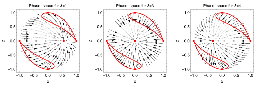
Figure 1: Phase-space portraits for the cosmological field equations of connection $\Gamma_{2}$ in the Poincare variables (41). The phase-space portraits are for $\lambda=1$, $\lambda=3$ and $\lambda=4$. With dots are the stationary points and red lines correspond to the family of points $B_{1}$. We observe that for $\lambda<3$, the unique attractor is the de Sitter solution described by point $B_{2}$.

Figure 2: Qualitative evolution of the equation of state parameter $w_{eff}^{\left(\Gamma_{2}\right)}$ for different values of $\lambda=\left(1,3,4\right)$ and for various initial conditions $\left(X_{0},Z_{0}\right)$. Solid lines are for $\left(0.95,0.1\right)$, dashed lines are for $\left(0.9,0.19\right)$, dotted lines are for $\left(0.8,0.3\right)$ and dash-dotted lines are for $\left(-0.8,0.3\right)$.

IV.3 Connection $\Gamma_{3}$

For the set of field equations related to the connection $\Gamma_{3}$ we introduce the dimensionless variables

$$\bar{x}=\frac{1}{2a^{2}H\dot{\Psi}}~{},~{}z=\frac{\dot{\zeta}}{H}~{},~{}y=\frac{V\left(\zeta\right)}{6H^{2}}~{},~{}\lambda=\frac{V_{,\zeta}}{V}~{},~{}\tau=\ln a,$$ (45)

that is,

$$\frac{1}{\dot{\Psi}}=2a^{2}\bar{x}H~{},~{}\dot{\zeta}=zH~{},~{}V\left(\zeta\right)=6yH^{2}~{},~{}V_{,\zeta}=\lambda V~{},~{}a=e^{\tau}.$$ (46)

The field equations read

$$\frac{d\bar{x}}{d\tau} =\frac{\bar{x}}{2z}\left(z\left(1+\bar{x}\right)-3+y\left(3-2\lambda\left(1-z\right)\right)\right),$$ (47)

$$\frac{dz}{d\tau} =3+\left(3-\bar{x}\right)z+y\left(\lambda\left(2+z\right)-3\right),$$ (48)

$$\frac{dy}{d\tau} =y\left(6+\lambda\left(2y+z\right)\right),$$ (49)

$$\frac{d\lambda}{d\tau} =\lambda^{2}z\left(\Gamma\left(\lambda\right)-1\right)~{},~{}\Gamma\left(\lambda\left(\zeta\right)\right)=\frac{V_{,\zeta\zeta}V}{\left(V_{,\zeta}\right)^{2}},$$ (50)

and constraint

$$1+y+\left(1+\bar{x}\right)z=0.$$ (51)

Moreover, the equation of state parameter is expressed as

$$w_{eff}^{\Gamma_{3}}=1+\frac{2}{3}\lambda y.$$ (52)

We remark that for the exponential potential $\lambda$ is always constant. Hence the stationary points $C=\left(C\left(\bar{x}\right),C\left(z\right),C\left(y\right)\right)$ for the latter algebraic-differential system are

$$C_{1}=\left(0,-1,0\right)~{},~{}C_{2}=\left(0,\frac{2}{\lambda}\left(3-\lambda\right),1-\frac{6}{\lambda}\right).$$ (53)

Point $C_{1}$ describes a stiff fluid solution, with $w_{eff}^{\Gamma_{3}}\left(C_{1}\right)=1$. On the other hand, the asymptotic solution at point $C_{2}$ describes an ideal gas with equation of state parameter $w_{eff}^{\Gamma_{3}}\left(C_{2}\right)=-3+\frac{2}{3}\lambda$. The stationary point describes acceleration for $\lambda<4$, while the cosmological constant is recovered for $\lambda=3$.

We make use of the constraint equation(51) and we reduce by one the dimension of the dynamical system. The eigenvalues of the linearized system around the stationary points $C_{1}$ and $C_{2}$ are $\left\{2,6-\lambda\right\}$; $\left\{\lambda-6,\frac{1}{2}\left(3\lambda-14\right)\right\}$ respectively. Therefore, point $C_{1}$ is a saddle point when $\lambda>6$, otherwise is a source; while point $C_{2}$ is an attractor for $\lambda<\frac{14}{3}$. We remark that when $C_{2}$ describes acceleration it is always attractor.

IV.3.1 Poincare variables

For the analysis at the infinity regime we work in the two-dimensional space defined by the dynamical variables $\left\{\bar{x},z\right\}$.

The Poincare variables are defined as

$$\bar{x}=\frac{\bar{X}}{\sqrt{1-\bar{X}^{2}-Z^{2}}}~{},~{}z=\frac{Z}{\sqrt{1-\bar{X}^{2}-Z^{2}}}~{},~{}dT=\sqrt{1-\bar{X}^{2}-Z^{2}}d\tau,$$

where $\left\{\bar{X}^{2},Z^{2}\right\}\leq 1$.

The field equations are reduced to the system of the form

$$\frac{dX}{dT}=F_{1}\left(X,Z\right)~{},~{}\frac{dZ}{dT}=F_{2}\left(X,Z\right),$$ (54)

and the equation of state parameter is expressed as

$$w_{eff}^{\Gamma_{3}}=1-\frac{2}{3}\lambda\left(1+\frac{Z\left(\bar{X}+\sqrt{1-X^{2}-Z^{2}}\right)}{1-X^{2}-Z^{2}}\right).$$ (55)

The stationary points $C^{\infty}=\left(X\left(C^{\infty}\right),Z\left(C^{\infty}\right)\right)$ at the infinity; that is, $1-\left(X\left(C^{\infty}\right)\right)^{2}-\left(Z\left(C^{\infty}\right)\right)^{2}=0$, are

$$C_{1\pm}^{\infty}=\left(0,\pm 1\right).$$

We calculate $w_{eff}^{\Gamma_{3}}\left(C_{1\pm}^{\infty}\right)=\mp\lambda\infty$. Hence, for $\lambda>0$, $C_{1+}^{\infty}$ corresponds to a Big Rip singularity, and $C_{1-}^{\infty}$ to a Big Crunch; nevertheless for $\lambda<0$, $C_{1+}^{\infty}$ corresponds to a Big Crunch singularity, and $C_{1-}^{\infty}$ to a Big Rip singularity.

The eigenvalues of the linearized system around the stationary points are $\left\{\pm 2\lambda,0\right\}$. Because the second eigenvalue is zero, we employ the CMT and we found that the stationary points does not posses any submanifold where the solutions are stable. Thus, the stationary points are saddle points or sources.

In Fig. 3 we present phase-space portraits for the dynamical system in Poincare variables. Furthermore, in Fig. 2 we present qualitative evolution of the equation of state parameter for various sets of initial conditions.

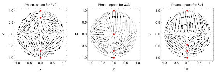
Figure 3: Phase-space portraits for the cosmological field equations of connection $\Gamma_{3}$ in the Poincare variables (41). The phase-space portraits are for $\lambda=2$, $\lambda=3$ and $\lambda=4$. With dots are the stationary points. We observe that the unique attractor is point $C_{2}$, while the two stationary points at the infinity regime are saddle points.

Figure 4: Qualitative evolution of the equation of state parameter $w_{eff}^{\left(\Gamma_{3}\right)}$ for different values of $\lambda=\left(2,2.5,3\right)$ and for various initial conditions $\left(X_{0},Z_{0}\right)$. Solid lines are for $\left(-0.95,0.05\right)$, dashed lines are for $\left(-0.8,0.2\right)$, dotted lines are for $\left(0.8,-0.2\right)$ and dash-dotted lines are for $\left(0.5,0.7\right)$.

V Conclusions

We conducted a detailed analysis of the asymptotic dynamics for an extension of STGR in which nonlinear components of the boundary term are introduced in the gravitational integral. In STGR, the definition of the connection is not unique, and for the spatially flat FLRW, there are three families of different connections. Although the selection of the connection does not affect the gravitational model in STGR when nonlinear terms of the boundary scalar are introduced, new dynamical degrees of freedom appear. The new degrees of freedom can be attributed to scalar fields, leading to three different sets of gravitational field equations, corresponding to the families of connections.

For the three different models, we employed dimensionless variables and determined the stationary points. We reconstructed the asymptotic solutions at the stationary points and investigated their stability properties. The results are summarized in Table 1.

The three gravitational models admit asymptotic solutions that can describe late-time acceleration. However, for connections $\Gamma_{2}$ and $\Gamma_{3}$, asymptotic solutions appear that can describe Big Rip or Big Crunch singularities. For connection $\Gamma_{2}$, a Big Crunch singularity is stable when the parameter $\lambda>3$. Thus, in this case, for the unique attractor to be the de Sitter solution, it follows that $\lambda\leq 3$. However, for these two specific models, the phase-space analysis leads to the derivation of sets for the initial conditions to avoid the appearance of such types of singularities.

The $Q+f\left(B\right)$ theory provides a mechanism to explain the late-time acceleration phase of the universe. Nevertheless, it is not obvious from this analysis if this theory can describe other eras of the cosmological history and if it solves the $H_{0}$-tension. In a future study, we plan to investigate this specific problem in the context of $f\left(Q,B\right)$-gravity.

Table 1: Asymptotic solutions in STGR with boundary correctons

Point	$\mathbf{w}_{eff}$	Acceleration	Stability
Connection $\mathbf{\Gamma}_{1}$
$A_{1}$	$1$	No	Stable$~{}\lambda>6$
$A_{2}$	$-3+\frac{2}{3}\lambda$	$\lambda<4$	Stable$~{}\lambda<6$
Connection $\mathbf{\Gamma}_{2}$
$B_{1}$	$1$	No	Unstable
$B_{2}$	$-1$	Yes	Stable
$B_{1\pm}^{\infty}$	$-1$	No	Unstable
$B_{2\pm}^{\infty}$	$\mp\infty$	Big Rip $B_{2+}^{\infty}$	$B_{2-}^{\infty}~{}$Stable $\lambda>3$
$B_{3\pm}^{\infty}~{}\left(\lambda=3\right)$	$\mp\infty$	Yes	Stable
Connection $\mathbf{\Gamma}_{3}$
$C_{1}$	$1$	No	Unstable
$C_{2}$	$-3+\frac{2}{3}\lambda$	$\lambda<4$	Stable $\lambda<\frac{14}{3}$
$C_{1\pm}^{\infty}$	$\mp\lambda\infty$	Big Rip	Unstable

References

• (1) A.G. Riess et al., Astron. J. 116, 1009 (1998)
• (2) M. Tegmark et al., Astrophys. J. 606, 702 (2004)
• (3) E. Komatsu et al., Astrophys. J. Suppl. Ser. 180, 330 (2009)
• (4) S. Nojiri, S.D. Odintsov and V.K. Oikonomou, Phys. Rept. 692, 1 (2017)
• (5) T. P. Sotiriou and V. Faraoni, Rev. Mod. Phys. 82 451, (2010)
• (6) S. Bahamonde, K. F. Dialektopoulos, C.ย Escamilla-Rivera,ย G.ย Farrugia, V. Gakis, M. Hohmann, J. L. Said, J. Mifsud and E. Di Valentino, Rep. Prog. Phys. 86, 026901 (2023)
• (7) H.A. Buchdahl, Mon. Not. Roy. Astron. Soc. 150, 1 (1970)
• (8) R. Ferraro and F. Fiorini, Phys. Rev. D 75, 084031 (2007)
• (9) J. B. Jimenez, L. Heisenberg and T. Koivisto, Phys. Rev. D 98, 044048 (2018)
• (10) S. M. Carrol, V. Duvvuri, M. Trodden and M. S. Turner, Phys. Rev. D., 70, 043528 (2004);
• (11) L.ย Amendola, D.ย Polarski and S.ย Tsujikawa, Phys.ย Rev.ย Lett.ย 98, 131302 (2007)
• (12) T. Clifton and J.D. Barrow, Class. Quant. Grav. 23, 2951 (2006)
• (13) R.C. Nunes, A. Bonilla, S. Pan and E.N. Saridakis, EPJC 77, 230 (2017)
• (14) A. de la Cruz-Dombriz, A. Dobado and A. L. Maroto, Phys. Rev. D 80, 124011 (2009)
• (15) J. Aftergood and A. DeBenedictis, Phys. Rev.ย D 90, 124006 (2014)
• (16) A. Lymperis, JCAP 11, 018 (2022)
• (17) S.H. Shekh, Phys. Dark Univ. 33, 100850 (2021)
• (18) F.K. Anagnastopoulos, S.ย Basilakos and E.N. Saridakis, Phys. Lett. B 822, 136634 (2021)
• (19) W.ย Hu and I. Sawicki, Phys. Rev. D. 76, 064004 (2007)
• (20) M. Krssak, R. J. van den Hoogen, J. G. Pereira, C. G. Boehmer and A. A. Coley, Class. Quantum Grav. 36, 183001 (2019)
• (21) M. Tsamparlis and A. Paliathanasis, Symmetry 10, 233 (2018)
• (22) K. Dialektopoulos, J.L. Said, Z. Oikonomopoulou, Eur. Phys. J. C 82, 259 (2022)
• (23) A.R. Akbarieh, P.S. Ilkhchi and Y. Kucukakca, Int. J. Geom. Meth. Mod. Phys. 20, 2350106 (2023)
• (24) S. Hembron, R. Bhaumik, S. Dutta and S. Chakraborty, Eur. Phys. J. C 84, 110 (2024)
• (25) S. Cotsakis and P.G.L. Leach, J. Phys. A: Math. Gen. 27, 1625 (1994)
• (26) J. Demaret and C. Scheen, J. Math. Phys. A: Math. Gen. 29, 59 (1996)
• (27) A. Paliathanasis, J.D. Barrow and P.G.L.ย Leach, Phys. Rev. D 94, 023525 (2016)
• (28) C.R Fadragas and G. Leon, Class. Quantum Grav. 31, 195011 (2014)
• (29) R. Lazkoz and G. Leon, Phys. Lett. B 638, 303 (2006)
• (30) T. Gonzales, G. Leon and I. Quiros, Class. Quantum Grav. 23, 3165 (2006)
• (31) A.A. Coley, Phys.ย Rev. D 62, 023517 (2000)
• (32) H. Farajollahi and A. Salehi, JCAP 07, 036 (2011)
• (33) E.J. Copeland, A.R. Liddle and D. Wands, Phys. Rev. D 57, 4686 (1998)
• (34) P. Christodoulidis, D. Roest and E.I. Sfakianakis, Scaling attractors in multi-field inflation, JCAP 12, 059 (2019)
• (35) L. Amendola, D.ย Polarski and S. Tsujikawa, IJMPD 16, 1555 (2007)
• (36) L. Amendola, D. Polarski and S. Tsujikawa, Phys. Rev. Lett. 98, 131302 (2007)
• (37) L. Amendola, R. Gannouji, D. Polarski and S. Tsujikawa, Phys.ย Rev. Dย 75, 083504 (2007)
• (38) J.M. Nester and H-J Yo, Chinese Journal of Physics 37, 113 (1999)
• (39) C.G. Boehmer and E. Jensko, Phys. Rev. D 104, 024010 (2021)
• (40) S. Capozziello, V. De Falco and C. Ferrara, Eur. Phys. J. C. 83, 915 (2023)
• (41) A.ย De, T.-H. Loo and E.N. Saridakis, Non-metricity with bounday terms: f(Q,C) gravity and cosmology, (2023) [arXiv:2308.00652]
• (42) L. Heisenberg, Phys. Reports 796, 1 (2019) lav2,lav3
• (43) J.B. Jimenez, L. Heisenberg, T. Koivisto and S. Pekar, Phys. Rev. D 101, 103507 (2020)
• (44) S. Bahamonde, C.G. Bohmer and M. Wright, Phys. Rev. D 10, 104042 (2015)
• (45) M. Wright, Phys. Rev. D 93, 103002 (2016)
• (46) M. Caruana, G. Farrugia and J.L.ย Said, EPJC 80, 640 (2020)
• (47) S. Bahamonde, A. Golovnev, M.-J. Guzmรกn, J.L. Said and C. Pfeifer, JCAP 01, 037 (2022)
• (48) A. Paliathanasis, JCAP 1708, 027 (2017)
• (49) A.ย Paliathanasis and G. Leon, EPJC 81, 718 (2021)
• (50) A. Paliathanasis, Phys. Dark Univ. 43, 101388 (2024)
• (51) F. Dโ€™ Ambrosio, L. Heisenberg and S. Kuhn, Class. Quantum Grav. 39 025013 (2022)
• (52) D. Zhao, Eur. Phys. J. C 82, 303 (2022)