Deep autoregressive density nets vs neural ensembles for model-based offline reinforcement learning

Abstract

We consider the problem of offline reinforcement learning where only a set of system transitions is made available for policy optimization. Following recent advances in the field, we consider a model-based reinforcement learning algorithm that infers the system dynamics from the available data and performs policy optimization on imaginary model rollouts. This approach is vulnerable to exploiting model errors which can lead to catastrophic failures on the real system. The standard solution is to rely on ensembles for uncertainty heuristics and to avoid exploiting the model where it is too uncertain. We challenge the popular belief that we must resort to ensembles by showing that better performance can be obtained with a single well-calibrated autoregressive model on the D4RL benchmark. We also analyze static metrics of model-learning and conclude on the important model properties for the final performance of the agent.

1 Introduction

Reinforcement learning consists in learning a control agent (policy) by interacting with a dynamical system (environment) and collecting its feedback (rewards). This learning paradigm turned out to be able to solve some of the world’s most difficult problems (Silver et al., 2017; 2018; Mnih et al., 2015; Vinyals et al., 2019). However, the scope of the systems that RL is capable of solving remains restricted to the simulated world and does not extend to real engineering systems. Two of the main reasons are i) small data due to operational constraints and ii) safety standards of such systems. In an attempt to bridge the gap between RL and engineering systems, we motivate the setting of offline reinforcement learning (Levine et al., 2020).

Offline reinforcement learning removes the need to query a dynamical system by using a previously collected dataset of controller-system interactions. In this optic, we view this setting as a supervised learning problem where one tries to approximate the underlying distribution of the data at hand, and hopefully be able to generalize to out-of-distribution samples. This turns out to be a difficult task for classical RL algorithms because of the distribution shift that occurs between the dataset and the learned policy during the learning process (Fujimoto et al., 2019; Levine et al., 2020). Thus we need to design algorithms that are well-suited for offline reinforcement learning. A common idea in this field is conservatism where one would only consider the learned agent when the input states are close to the support of the offline dataset. Depending on the algorithm, conservatism can take multiple forms, ranging from penalized Q-targets (Kumar et al., 2020) to uncertainty-penalized Markov decision processes (Kidambi et al., 2020; Yu et al., 2020). To develop further into this direction, we make the distinction between model-free and model-based RL (MBRL) algorithms.

Model-free algorithms learn a policy and/or a value function by observing the reward signal realizations and the underlying dynamics of the system, which in most environments requires a significant number of interactions for achieving good performance (Haarnoja et al., 2018). In this category, a way to incorporate conservatism is to penalize the value targets of data points that are distant from the offline dataset (Kumar et al., 2020). Other methods include behavior regularized policy optimization (Wu et al., 2020).

Model-based algorithms are composed of two independent (and often alternating) steps: i) model learning: a supervised learning problem of learning the dynamics (and sometimes also the reward function) of the system of interest; and ii) policy optimization, where we sample from the learned dynamics to learn a policy and/or a value function. MBRL is known to be sample-efficient, since policy/value learning is done (completely or partially) from imaginary model rollouts (also called background planning) that are cheaper and more accessible than rollouts in the true dynamics (Janner et al., 2019). Furthermore, a predictive model with good out-of-distribution performance affords easy transfer of the true model to new tasks or areas not covered in the offline dataset (Yu et al., 2020). Conservatism in MBRL is frequently achieved by uncertainty-based penalization of the model predictions. This relies on well-calibrated estimation of the epistemic uncertainty of the learned dynamics, which is a limitation of this approach.

It is of great interest to build models that know when (and how much) they do not know, thus uncertainty estimation remains a central problem in MBRL. Many recent works have made progress in this direction (Osband et al., 2021). The most common approach to date is bootstrap ensembles: we construct a population of predictive models (most often probabilistic neural networks) and consider disagreement metrics as our uncertainty measurement. The source of randomness in this case is the random initialization of the parameters of neural networks and the subset of the training data that each model sees. When the environment is stochastic, ensembles help to separate the aleatory uncertainty (intrinsic randomness of the environment) and the epistemic uncertainty (Chua et al., 2018). When the environment is deterministic (which is the case of the D4RL Mujoco benchmark environments considered in most of the offline RL literature (Fu et al., 2021a)), the error is fully epistemic: it consists of the estimation error (due to lack of training data) and the approximation error (mismatch between the model class and the true distribution) (Hüllermeier & Waegeman, 2021). This highlights the need of well-calibrated probabilistic models whose posterior variance can be used as an uncertainty measurement in conservative MBRL.

In this work, we propose to compare autoregressive dynamics models (Uria et al., 2016) to ensembles of probabilistic feedforward models, both in terms of static evaluation (supervised learning metrics on the task of learning the system dynamics) and dynamic evaluation (final performance of the MBRL agent that uses the model). Autoregressive models learn a conditional distribution of each dimension of the next state conditioned on the input of the model (current state and action) and the previously generated dimensions of the next state. Meanwhile, probabilistic feedforward models learn a multivariate distribution of the next state conditioned on the current state and action. We argue that autoregressive models can learn the implicit functional dependence between state dimensions, which makes them well-calibrated, leading to good uncertainty estimates suitable for conservatism in MBRL.

Our key contributions are the following.

• We apply autoregressive dynamics models in the context of offline model-based reinforcement learning and show that they improve over neural ensembles in terms of static evaluation metrics and the final performance of the agent.

• We introduce an experimental setup that decouples model selection from agent selection to reduce the burden of hyperparameter optimization in offline RL.

• We study the impact of static metrics on the dynamic performance of the agents, and conclude on the importance of single-step calibratedness in model-based offline RL.

2 Related work

Offline RL has been an active area of research following its numerous applications in domains such as robotics (Chebotar et al., 2021), healthcare (Gottesman et al., 2018), recommendation systems (Strehl et al., 2010), and autonomous driving (Kiran et al., 2022). Despite outstanding advances in online RL (Haarnoja et al., 2018; Silver et al., 2017; Mnih et al., 2015) and iterated offline RL (Wang et al., 2019; Wang & Ba, 2020; Matsushima et al., 2021; Kégl et al., 2021), offline RL remained a challenging problem due to the dependency on the data collection procedure and its potential lack of exploration (Levine et al., 2020).

Although any off-policy model-free RL agent can theoretically be applied to offline RL (Haarnoja et al., 2018; Degris et al., 2012; Lillicrap et al., 2016; Munos et al., 2016), it has been shown that these algorithms suffer from distribution shift and yield poor performance (Fujimoto et al., 2019; Levine et al., 2020). To alleviate the problem of distribution shift, conservatism was introduced successfully by several techniques, such as BEAR (Kumar et al., 2019), AlgaeDICE (Nachum et al., 2019), AWR (Peng et al., 2020), BRAC (Wu et al., 2020), and CQL Kumar et al. (2020). The general objective of these methods is to keep the model-free policy close to the behavioral policy, in other words, to avoid wandering into regions of the state/action space where no data was collected.

Model-based RL has been successfully applied to the online RL setting by alternating model learning and planning (Deisenroth & Rasmussen, 2011; Hafner et al., 2021; Gal et al., 2016; Levine & Koltun, 2013; Chua et al., 2018; Janner et al., 2019; Kégl et al., 2021). Planning is done either decision-time via model-predictive control (Draeger et al., 1995; Chua et al., 2018; Hafner et al., 2019; Pinneri et al., 2020; Kégl et al., 2021)), or Dyna style by learning a model-free RL agent on imagined model rollouts (Janner et al., 2019; Sutton, 1991; Sutton et al., 1992; Ha & Schmidhuber, 2018). For instance, MBPO (Janner et al., 2019) trains an ensemble of feed-forward models and generates imaginary rollouts to train a soft actor-critic, which policy is then used to generate new data for model learning. MBPO has been showed to achieve state of the art in continuous control task with the smallest sample efficiency. An adaptation of MBPO to the offline setting is MOPO (Yu et al., 2020). MOPO incorporates conservatism via a surrogate MDP where the rewards are penalized with the uncertainty of the model. While MOPO relies on disagreement metrics between the members of the learned ensemble, we suggest the use of well-calibrated autoregressive models whose learned variance is a good proxy to the model estimation error. Similar uncertainty penalized policy search is used in a number of other works (Kidambi et al., 2020; Lee et al., 2021; Shen et al., 2021; Swazinna et al., 2021; Depeweg et al., 2018), while others explore pessimism-based decision time planning (Argenson & Dulac-Arnold, 2021; Zhan et al., 2021), conservative value learning (Yu et al., 2021; Liu et al., 2021).

Autoregressive models have been studied in a number of previous works for generative modeling in general (Uria et al., 2016; 2013; Papamakarios et al., 2017; Van Den Oord et al., 2016). However, only a handful of papers use them in the context of MBRL (Kégl et al., 2021; Zhang et al., 2021b; Zhan et al., 2021). Zhang et al. (2021b) used autoregressive models for model-based off-policy evaluation, while we focus our study on the important model properties for offline policy optimization. We also adapt metrics from Kégl et al. (2021) to provide a complete guide on model selection for offline MBRL.

Previous works have tackled hyperparameter selection in online RL (Andrychowicz et al., 2021; Engstrom et al., 2020), MBRL (Zhang et al., 2021a), and offline RL (Paine et al., 2020), showing the sensibility of existing algorithms to hyperparameter choices. Lu et al. (2022) perform a similar analysis to this work. Similarly to us, they base their analysis on MOPO, but they focus on the uncertainty-related hyperparameters while we revisit the model design and architecture.

3 Preliminaries

The standard framework of RL is the finite-horizon Markov decision process (MDP) $\mathcal{M}=\langle\mathcal{S},\mathcal{A},p,r,\mu_{0},\gamma\rangle$ where $\mathcal{S}$ represents the state space, $\mathcal{A}$ the action space, $p:\mathcal{S}\times\mathcal{A}\mathrel{\text{\char 59\relax}}\mathcal{S}$ the (possibly stochastic) transition dynamics, $r:\mathcal{S}\times\mathcal{A}\rightarrow\mathbb{R}$ the reward function, $\mu_{0}$ the initial state distribution, and $\gamma\in[0,1]$ the discount factor. The goal of RL is to find, for each state $s\in{\cal S}$, a distribution $\pi(s)$ over the action space ${\cal A}$, called the policy, that maximizes the expected sum of discounted rewards $J(\pi,\mathcal{M}):=\mathbb{E}_{s_{0}\sim\mu_{0},a_{t}\sim\pi,\,s_{t>0}\sim p}[\sum_{t=0}^{H}\gamma^{t}r(s_{t},a_{t})]$, where $H$ is the MDP horizon. Under a policy $\pi$, we define the state-action value function (Q-function) at an $(s,a)\in{\cal S}\times{\cal A}$ pair as the expected sum of discounted rewards, starting from the state $s$, taking the action $a$, and following the policy $\pi$ afterwards until termination: $Q^{\pi}(s,a)=\mathbb{E}_{a_{t>0}\sim\pi,s_{t>0}\sim p}\big{[}\sum_{t=0}^{H}\gamma^{t}r(s_{t},a_{t})\mid s_{0}=s,a_{0}=a\big{]}$. We can similarly define the state value function by taking the expectation with respect to the initial action $a_{0}$: $V^{\pi}(s)=\mathbb{E}_{a_{t}\sim\pi,s_{t>0}\sim p}\big{[}\sum_{t=0}^{H}\gamma^{t}r(s_{t},a_{t})\mid s_{0}=s\big{]}$.

In offline RL, we are given a set of transitions $\mathcal{D}=\{(s_{t}^{i},a_{t}^{i},r_{t}^{i},s_{t+1}^{i})\}_{i=1}^{N}$, where $N$ is the size of the set, generated by an unknown behavioral policy $\pi^{\beta}$. The difficulty of offline RL comes from the fact that we are not allowed to interact further with the environment $\mathcal{M}$ even though we aim to optimize the objective $J(\pi,\mathcal{M})$ with $\pi\not=\pi^{\beta}$. In practice, the current offline RL algorithms are still provided with an online evaluation budget, a setting we will follow in the rest of the paper. The question of offline policy evaluation (or budget-limited policy evaluation) is an active research direction (see, e.g., Fu et al. (2021b)) and is beyond the scope of this paper.

Model-based RL algorithms use an offline dataset $\mathcal{D}$ to solve the supervised learning problem of estimating the dynamics of the environment $\hat{p}$ and/or the reward function $\hat{r}$. For various reasons (stochastic environment, ability to represent the uncertainty of the predictions), the loss function is usually the log-likelihood $\mathcal{L}(\mathcal{D};\hat{p})=\frac{1}{N}\sum_{i=1}^{N}\log\hat{p}(s^{i}_{t+1}|s^{i}_{t},a^{i}_{t})$. The learned model can then be used for policy search under the MDP $\hat{\mathcal{M}}=\langle\mathcal{S},\mathcal{A},\hat{p},\hat{r},\mu_{0},\gamma\rangle$, which has the same state and action spaces $\mathcal{S},\mathcal{A}$ as the true environment $\mathcal{M}$, but which has the transition probability $\hat{p}$ and the reward function $\hat{r}$ that are learned from the offline data $\mathcal{D}$. The obtained optimal policy $\hat{\pi}=\mathop{\rm argmax}_{\pi}J(\pi,\hat{\mathcal{M}})$ is not guaranteed to be optimal under the true MDP $\mathcal{M}$ due to distribution shift and model bias. $J(\pi,\hat{\mathcal{M}})$ and $J(\pi,\mathcal{M})$ are somewhat analogous to training and test scores in supervised learning, with two fundamental differences: i) they are only loosely connected to the actual supervised loss $\mathcal{L}(\mathcal{D};\hat{p})$ that we can optimize and measure on a data set, and ii) because we are not allowed to collect data using $\pi$, there is a distribution shift between training and test.

Regarding the type of model, the usual choice is a probabilistic model that learns the parameters of a multivariate Gaussian over the next state and reward, conditioned on the current state and action: $s_{t+1},r_{t}\sim\hat{p}_{\theta}(.|s_{t},a_{t})=\mathcal{N}\big{(}\mu_{\theta}(s_{t},a_{t}),\sigma_{\theta}(s_{t},a_{t})\big{)}$, where $\theta$ represents the parameters of the predictive model. In practice, we use fully connected neural networks as they are proved to be powerful function approximators (Nagabandi et al., 2018; Chua et al., 2018), and for their suitability to high-dimensional environments over simpler non-parametric models such as Gaussian processes. Following previous work (Chua et al., 2018), we assume a diagonal covariance matrix for which we learn the logarithm of the diagonal entries: $\sigma_{\theta}=\mathrm{Diag}(\exp(l_{\theta}))$ with $l_{\theta}$ output by the neural network.

One of the conditions of such a joint model is the conditional independence of the dimensions of the predicted state, which is a strong assumption, especially in the case of functional (or physical) dependency. $y$-interdependence (Kégl et al., 2021) happens, for example, when angles are represented by sine and cosine. For this purpose, we study autoregressive models that learn a single model per dimension, conditioned on the input of the model $(s_{t},a_{t})$ and the previously generated dimensions. Formally, $\hat{p}_{\theta}(s_{t+1}|s_{t},a_{t})=\hat{p}_{\theta_{1}}(s^{1}_{t+1}|s_{t},a_{t})\prod^{d_{s}}_{j=2}\hat{p}_{\theta_{j}}(s^{j}_{t+1}|s^{1}_{t+1},\ldots,s^{j-1}_{t+1},s_{t},a_{t})$, where $d_{s}$ is the dimension of the state space ${\cal S}$.

Conservatism in MBRL requires an uncertainty estimate $\hat{u}(s,a)$ reflecting the quality of the model in different regions of the state/action space. For this purpose, probabilistic models provide an uncertainty estimate by learning the variance of the predictions (in this case under a Gaussian distribution). In noisy environments, this uncertainty estimate represents both the aleatory uncertainty (intrinsic randomness of the environment) and the epistemic uncertainty (model estimation and approximation errors). Conservative MBRL uses the epistemic uncertainty only, so, in practice, the problem of separating the aleatory uncertainty and the epistemic uncertainty is addressed through the use of bootstrap ensembles (Chua et al., 2018). Ensembling consists in having $D\in\mathbb{N}^{*}-\{1\}$ models, each initialized randomly and trained on a set $\mathcal{D}_{\ell}$ for $\ell\in\{1,\ldots,D\}$ generated by sampling with replacement from a common dataset $\mathcal{D}$. Using ensembles, we can compute a disagreement metric to capture the epistemic uncertainty, as opposed to the aleatory uncertainty learned by each member of the ensemble. A detailed discussion about these uncertainty heuristics is provided in Section 4.

4 A baseline: model-based offline policy optimization (MOPO)

Models $\hat{p}$ in MBRL are not used in isolation. Their likelhood ratio, precision, and calibratedness (LR, R2, and KS in Section 5.1 and Appendix C) are good proxies, but ultimately their quality is judged when they are used in a policy. To compare the dynamic performance of the models $\hat{p}$, we fix the policy to MOPO (Yu et al., 2020), a conservative agent-learning algorithm. MOPO uses a pessimistic MDP (P-MDP) to ensure that the performance of the policy with the model will be a lower bound of the performance of the policy on the real system. Yu et al. (2020) show a theoretical lower bound on the true return based on the estimation error of the learned dynamics $J(\pi,\mathcal{M})\geq\mathbb{E}_{a\sim\pi,\,s\sim\hat{p}}\big{[}r(s,a)-\gamma|G^{\pi}_{\hat{\mathcal{M}}}(s,a)|\big{]}$. In this formula, $G^{\pi}_{\hat{\mathcal{M}}}(s,a)$ is defined by $\mathbb{E}_{s^{\prime}\sim\hat{p}(s,a)}[V^{\pi}_{\cal M}(s^{\prime})]-\mathbb{E}_{s^{\prime}\sim p(s,a)}[V^{\pi}_{\cal M}(s^{\prime})]$ which quantifies the effect of the model error on the return. However, this requires access to the value function of the policy $\pi$ under the true MDP ${\cal M}$, which is not given in practice.

To derive an algorithm based on this theoretical bound, MOPO relies on an upper bound of $G^{\pi}_{\hat{\mathcal{M}}}(s,a)$ based on the integral probability metric: $G^{\pi}_{\hat{\mathcal{M}}}(s,a)\leq\sup_{f\in\mathcal{F}}\mid\mathbb{E}_{s^{\prime}\sim\hat{p}}[f(s^{\prime})]-\mathbb{E}_{s^{\prime}\sim p}[f(s^{\prime})]\mid$, where $\mathcal{F}$ is an arbitrary set of functions. In practice, the authors use ensemble-based uncertainty heuristics to set an upper bound on the true error of the model. The maximum standard deviation among the ensemble members (labeled max aleatory or MA) is considered to define a penalized reward $\tilde{r}(s,a)=\hat{r}(s,a)-\lambda\hat{u}(s,a)$, where $\hat{u}(s,a)=\max_{\ell=1,\ldots,N}\|\sigma^{\ell}_{\theta}(s,a)\|_{F}$ and $\lambda$ is a penalty hyperparameter. Yu et al. (2020) then define the associated P-MDP $\tilde{\mathcal{M}}=\langle\mathcal{S},\mathcal{A},\hat{p},\tilde{r},\mu_{0},\gamma\rangle$ on which a soft actor-critic (SAC) (Haarnoja et al., 2018) agent is trained until convergence (Algorithm 1). This algorithm is based on Model-based policy optimization (MBPO) (Janner et al., 2019) which alternates between model learning and agent learning. MOPO can be described as one iteration of MBPO, which learns the dynamics model (a bootstrap ensemble of probabilistic neural networks) from the offline dataset and then learns the off-policy agent on a buffer of rollouts in the P-MDP $\tilde{\mathcal{M}}$. Using this P-MDP prevents the agent from exploiting rewards of highly uncertain regions.

Data: Dataset ${\cal D}$, penalty coefficient $\lambda$, rollout horizon $h$, Number of SAC training batches $B$, conservatism penalty $\hat{u}(s,a)$.

Train dynamics model $\hat{p}$ on offline dataset ${\cal D}$;

Initialize SAC policy $\pi$ and empty replay buffer ${\cal D}_{model}$;

for $1,2,\ldots,B$ do

       Sample initial state $s_{0}$ from ${\cal D}$;

       for $i=1,2,\ldots,h$ do

             Sample an action $a_{i}\sim\pi(s_{i})$;

             Sample the next state from the dynamics model $s_{i+1},r_{i}\sim\hat{p}(s_{i},a_{i})$;

             Compute the penalized reward $\tilde{r}_{i}=r_{i}-\lambda\hat{u}(s_{i},a_{i})$;

             Add sample $(s_{i},a_{i},\tilde{r}_{i},s_{i+1})$ to ${\cal D}_{model}$;

            

       end for

      Draw a batch from ${\cal D}_{model}$, update $\pi$ following SAC schema;

      

end for

Algorithm 1 MOPO pseudocode. Yu et al. (2020) uses $\hat{u}(s,a)=\max_{\ell=1,\ldots,N}\|\sigma^{\ell}_{\theta}(s,a)\|_{F}$; we also experimented with two other penalty heuristics by Lu et al. (2022).

While Yu et al. (2020) only tried the max aleatory estimator for the uncertainty heuristic, Lu et al. (2022) introduced concurrent ensemble-based uncertainty heuristics from recent works and deployed them in MOPO. Among these, we chose the following two, showing competitive performance in benchmarks.

• Max pairwise difference (MPD) (Kidambi et al., 2020): $\hat{u}(s,a)=\max_{l,l^{\prime}}\|\mu^{l}_{\theta_{l}}(s,a)-\mu^{l^{\prime}}_{\theta_{l^{\prime}}}(s,a)\|_{2}$ for $l\neq l^{\prime}\in{1,\ldots,D}$. This metric captures the largest disagreement among ensemble members as an indicator of model error.

• Ensemble standard deviation (ESD) (Lakshminarayanan et al., 2017):
  $\hat{u}(s,a)=\sqrt{\frac{1}{D}\sum_{l}^{D}\left((\sigma^{l}_{\theta_{l}}(s,a))^{2}+(\mu^{l}_{\theta_{l}}(s,a))^{2}\right)-(\bar{\mu}(s,a))^{2}}$ with $\bar{\mu}(s,a)=\frac{1}{D}\sum_{l}^{D}\mu^{l}_{\theta_{l}}(s,a)$, is the standard deviation of the ensemble, i.e., the standard deviation of the equally-weighted mixture of the Gaussian densities.

5 Experimental setup

We implement our MOPO baseline based on the MBRL library released by Kégl et al. (2021) which is built on top of the RAMP framework (Kégl et al., 2018). We run our experiments with the following models:

• DARMDN($D$): Deep autoregressive mixture density net. $d_{s}\in\mathbb{N}^{*}$ feed-forward neural network that learn the parameters (mean and log-standard deviation), and the weights of $D\in\mathbb{N}^{*}$ univariate Gaussian distributions ($d_{s}$ being the dimension of the state space $\mathcal{S}$). Although our implementation is general, for the rest of the paper we only consider DARMDN(1) due to runtime bottleneck, we refer to it as simply DARMDN.

• DMDN($D$): Deep mixture density net. A feed-forward neural network that learns the parameters (mean and log-standard deviation) and the weights of $D\in\mathbb{N}^{*}$ multivariate Gaussian distributions. For similar reasons as DARMDN, we only consider DMDN(1) and refer to it as DMDN.

• ENS: Ensemble of $D\in\mathbb{N}^{*}$ DMDN models. We implement a vectorized version that is optimized to run on a Graphical Processing Units (GPUs). Notice that ENS is equivalent to the original model MOPO used, modulo architectural choices.

For the single models (DARMDN and DMDN), we consider their learned standard deviation ($\sigma_{\theta}$) as the uncertainty heuristic to use for reward penalization, which is equivalent to the max aleatory heuristic for an ensemble of a single member. For ENS, we follow the schema by Lu et al. (2022) and tune the uncertainty heuristic as an additional hyperparameter among MA, MPD, and ESD, defined in Section 4.

In a typical MBRL loop, the experimental setup consists of alternating model learning and agent learning until the potential convergence of the dynamic performance (episodic return) of the agent on the real environment. For computationally limited hyperparameter optimization, this setup provides continuous feedback on the return of a given model, which helps to early-stop unpromising experiments. This is not possible in single-iteration offline RL as we only have access to a static dataset for model learning, and we have to run all the pipeline to compute the evaluation score of a given model. For this purpose, we suggest to decouple model selection and agent selection in an attempt to reduce the overall computational budget of the approach. The experimental setup will then be separated to two independent parts:

• Static evaluation of the models: Starting from a dataset ${\cal D}$, we evaluate the different models by computing supervised-learning evaluation metrics (Sections 5.1 and C) on a held-out validation set. We then select the best model hyperparameters based on these metrics.

• Dynamic evaluation of the agents: After selecting the best model $\hat{p}$, we train agents by interacting with the P-MDP defined on the learned dynamics of the model. During training, we evaluate the agents by repeatedly rolling-out trajectories in the real environment and computing their average episodic return. For this purpose, we assume access to the true simulator at evaluation time, although the recorded episodes are not made available to training.

A limitation of this approach comes from the fact that static supervised learning metrics do not necessarily reflect the quality of the model for agent learning. We thus investigate how these static metrics predict the overall dynamic performance in Section 6.

5.1 Static metrics

We use metrics introduced by Kégl et al. (2021) in the context of iterated offline reinforcement learning. These metrics are designed to assess different aspects of model quality: precision, calibratedness, and sensitivity to compounding errors via long-horizon metrics.

Precision is evaluated using the explained variance (R2) which we prefer over the standard Mean-squared error (MSE) because it is normalized and can be aggregated over multiple dimensions. Calibratedness is measured using the Kolmogorov-Smirnov statistics (KS) between the ground truth validation quantiles and a uniform distribution. This metrics indicates if the ground truth values are distributed following the predicted distributions. In the Gaussian case, it is equivalent to the predicted standard deviation being in the order of magnitude of the true model error (although a bad KS may also indicate that the model errors are not Gaussian). We also use the likelihood ratio with respect to a baseline score (LR), and the outlier ratio (OR), the rate of data points on which the likelihood is close to zero. For the impact of compounding errors, we sample a population of trajectories (following ground truth actions) and compute Monte-Carlo estimates of the long-horizon metrics (R2($L$) and KS($L$) for $L\in\{1,\ldots,20\}$). The formal definition of these metrics can be found in Appendix C.

5.2 Dynamic metrics

Similarly to Kidambi et al. (2020); Wu et al. (2020), we compute the average episodic return (undiscounted sum of rewards) of the agent on the real system during training, formally $R(\{(s_{t},a_{t},r_{t},s_{t+1})\}_{t=1}^{H})=\sum_{t=1}^{H}r_{t}$ of the agent, where $H$ is the episode size. We then keep track of the agent with the highest return for the final evaluation. This is not what we should do if the goal was to develop a standalone offline RL algorithm (we could not use the real return to select the agent), but our goal in this paper is to compare models $\hat{p}$ of the system dynamics, so as long as the agent is selected in the same way for all the models, the comparison is fair.

We use the normalized scores introduced in the D4RL benchmark. This metric is a linear transformation of the episodic return and takes values between 0 and 100 with 0 corresponding to the score of a randomly initialized SAC agent, and 100 to a SAC agent that is trained until convergence on the real system.

6 Experiments & Results

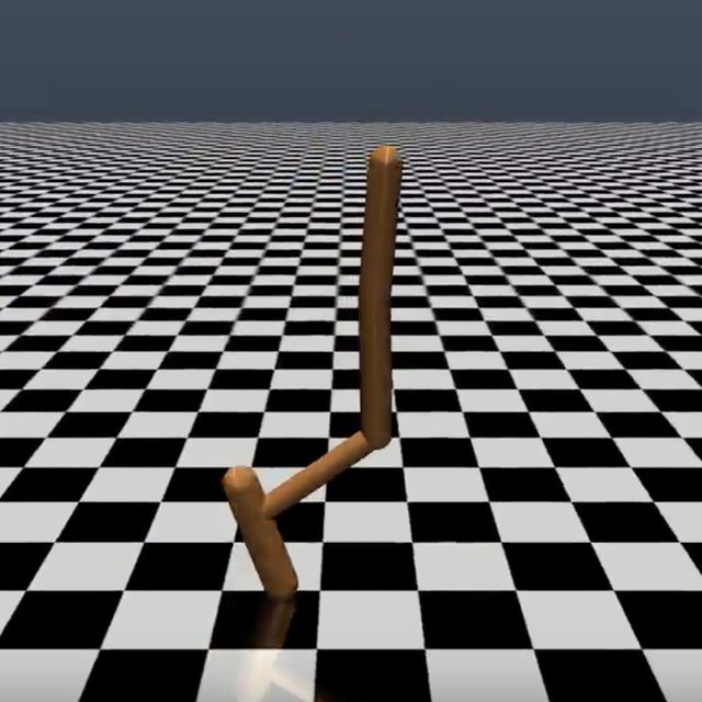
Figure 1: Hopper

All our experiments are conducted in the continuous control environment Hopper. We use the implementation of OpenAI Gym (Brockman et al., 2016) that is based on the Mujoco physics simulator (Todorov et al., 2012). A description of this environment can be found in Appendix B.

For static datasets, we use the D4RL Hopper benchmark that provides four static sets generated by different behavior policies (random: 1M steps generated by a randomly initialized SAC agent, medium: 1M steps generated by a SAC agent trained until half the score at convergence, medium-replay: All the traces collected by a SAC agent trained until half the score at convergence, medium-expert: 2M steps consisting of the medium dataset and 1M steps generated by an expert SAC agent).

The results of the static evaluation of the models are summarized in Table 1. The reported scores are validation scores on a held-out 10$\%$ validation set from the D4RL datasets.

Table 1: Model evaluation results on static datasets. $\downarrow$ and $\uparrow$ mean lower and higher the better, respectively. Unit is given after the $/$ sign.

Model	LR$\uparrow$	OR$/10^{-4}$$\downarrow$	R2$/10^{-4}$$\uparrow$	KS$/10^{-3}$$\downarrow$	R2(10)$/10^{-4}$$\uparrow$	KS(10)$/10^{-3}$$\downarrow$
	Hopper-v2, D4RL random dataset
DMDN	976	0	9986	146	8017	190
DARMDN	1141	0	9987	134	5011	377
ENS	304	1	9984	217	9442	190
	Hopper-v2, D4RL medium dataset
DMDN	1322	1	9998	117	9938	84
DARMDN	1473	2	9996	56	9586	112
ENS	341	1	9953	233	9296	143
	Hopper-v2, D4RL medium-replay dataset
DMDN	361	3	9990	120	9817	141
DARMDN	575	4	9986	65	9580	141
ENS	219	1	9928	190	6982	115
	Hopper-v2, D4RL medium-expert dataset
DMDN	-	-	-	-	-	-
DARMDN	1675	1	9996	59	8814	160
ENS	452	1	9976	227	9727	108

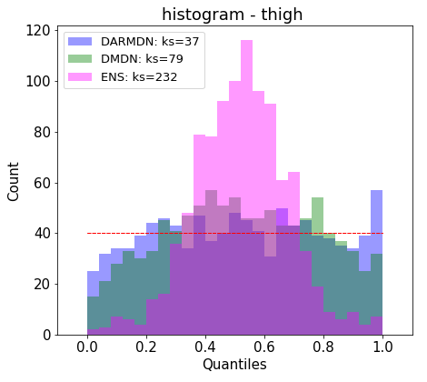
Figure 2: Histogram of Hopper’s thigh ground truth quantiles, under the model distribution (D4RL medium dataset). The legend also includes the value of the KS calibratedness metric. The dotted red line indicates the ideal case when the quantiles follow a uniform distribution.

One-step metrics (LR, OR, R2, and KS).

We first observed that single models are consistently better than the ensemble in terms of one-step metrics. To better understand this result, we propose to use the ground truth test quantiles as a debugging tool on the calibratedness of the models. Figure 2 and Appendix E show that the ensemble model overestimates its error because the ground truth values are concentrated around $0.5$. We suggest that this is because each DMDN ensemble member has a well-calibrated variance, but when we treat the ensemble as a mixture model, the variance of the mean adds to the individual variances, “diluting” the uncertainty. Regarding the comparison between DMDN and the autoregressive DARMDN, we observe that although they have similar R2 scores, DARMDN is consistently beating DMDN in terms of KS and LR which depend also on accurate and well-calibrated sigma estimates, an important property for conservative MBRL.

To push the analysis further, we suggest to look at the dimension-wise static metrics, reported in Appendix D. The results depend on the different datasets, yet some results are consistent and help explain the improvement that autoregressive models bring over their counterparts. For instance in three out of four datasets, the LR score of the thigh and thigh_dot dimensions is an order of magnitude higher for the autoregressive model. We suggest that this is due to the functional dependence that might exist between the different observables, which is easily captured by the autoregressive model as it uses the previously predicted dimensions as input to the next ones.

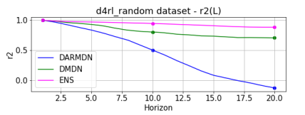
Figure 3: Long horizon explained variance R2($L$) in the D4RL random dataset.

Long-horizon metrics.

Unlike in single-step metrics, here we observe a significant degradation in the performance of DARMDN, both in terms of R2$(L)$ and KS$(L)$ for $L\in\{1,\ldots,20\}$ (Figure 3 and Appendix F). We suggest that this is the due to optimizing the models for single-step likelihood. Outliers (last bin of Figure 2) count little in the single-step likelihood, but may compound when recursing the model through $L$ steps.

Dynamic evaluation.

Table 2 shows the episodic return achieved by the best agent throughout one million steps of SAC training. SAC agents that were trained using DARMDN models performed better on the real system despite their suboptimal long-horizon performance. We suggest that for an agent that trained by one-step Q-learning, such as SAC, only one-step errors matter. Ensemble models improve over DMDN in the random dataset, but scores are comparable or worse in the remaining tasks, although none of the differences are highly significant (they depend on a couple of lucky seeds; a phenomenon that muddies the offline RL field). One result seems remarkable: DARMDN models seem to be able to consistently generate agents that go beyond Hopper simply standing up (score of about 30).

Table 2: Model dynamic evaluation: mean $\pm$ $90\%$ Gaussian Confidence Interval

over 3 seeds of the hyperoptimal SAC agents. The reported score is the D4RL normalized score explained in Section 5. D4RL dataset DARMDN DMDN ENS random 31.34 $\pm$ 0.41 17.54 $\pm$ 7.96 31.97 $\pm$ 0.21 medium 66.96 $\pm$ 5.14 33.12 $\pm$ 4.84 14.12 $\pm$ 10.76 medium_replay 70.57 $\pm$ 19.86 33.16 $\pm$ 1.54 28.96 $\pm$ 12.89 medium_expert 64.18 $\pm$ 20.39 - $\pm$ - 32.10 $\pm$ 0.54

Correlating static metrics and dynamic scores.

The experimental setup we introduce has the advantage of reducing the combinatorics of the hyperparameter optimization process. However, the best agents do not necessarily come from the models with the best static metrics, since these are measured on static data not representative of the distribution on which they are applied in the dynamic run. In an attempt to optimize model selection, we investigate the model properties (static metrics) that are most important for dynamic scores. For this, we compute Spearman rank correlation ($\rho$) and Pearson bivariate correlation ($r$) between the static score obtained for all models and their respective dynamic scores.

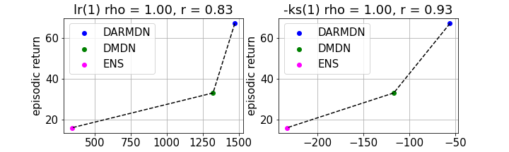
Figure 4: The Spearman and Pearson correlations between the episodic return and LR/-KS metrics on the D4RL medium dataset.

A value of $\rho=1$ indicates that the static metric conserves the same ranking observed in the dynamic evaluation (sufficient for model selection) while $r=1$ tells that the gap observed in the static metric is in the same scale of the one observed in the dynamic performance (linear correlation). The results in Figure 4 and Appendix G show that in most datasets, the two most correlating metrics are LR ($\rho=1.0$ and $r=0.93$) and KS$(1)$ ($\rho=1.0$ and $r=0.83$), metrics that evaluate the calibratedness of the models. This underlines the fact that autoregressive models yield the best agent because of their ability to learn one-step uncertainty estimates that represent well their true errors.

D4RL benchmark.

We compare the scores obtained with our best agent (based on an autoregressive model) with existing literature in the D4RL benchmark and include the results in Table 3.

Table 3: Results on the D4RL benchmark. The scores indicate the mean $\pm$ $90\%$ Gaussian confidence interval across 3 seeds (6 seeds for MOPO) of the normalized episodic return. We take the scores of MBRL algorithms from their respective papers, and the scores of the model free algorithms and Behavior cloning (BC) from the D4RL paper (Fu et al., 2021a).

D4RL dataset	BC	Ours	MOPO	COMBO	MOREL	SAC	BEAR	BRAC-v	CQL
random	1.6	31.3 $\pm$ 0.4	11.7 $\pm$ 0.1	17.9	53.6	11.3	9.5	12.0	10.8
medium	29.0	66.9 $\pm$ 5.1	28.0 $\pm$ 4.0	94.9	95.4	0.8	47.6	32.3	86.6
medium_replay	11.8	70.5 $\pm$ 19.8	67.5 $\pm$ 8.0	73.1	93.6	1.9	10.8	0.9	48.6
medium_expert	111.9	64.1 $\pm$ 20.3	23.7 $\pm$ 1.95	111.1	108.7	1.6	4.0	0.8	111.0

Our algorithm achieves better or similar (medium_replay) performance than MOPO, suggesting that potentially the improvement is brought by autoregressive models over neural ensembles, which supports the case of single well-calibrated models. However, we would like to emphasize that there may be other potential reasons behind such differences of performance. For instance Kidambi et al. (2020) append the observations with the unobserved x_velocity to get access to the full state of the true MDP. The D4RL dataset version (v0 or v2) has also been criticized as providing different qualities for the same dataset (we use v2 similar to Kidambi et al. (2020) and Yu et al. (2021) while Yu et al. (2020) uses v0). Another important point is the evaluation protocol that sometimes assumes access to the real system for policy evaluation (Kidambi et al., 2020; Wu et al., 2020; Fujimoto et al., 2019; Kumar et al., 2019), and sometimes only reports the online evaluation score of the policy at the last agent-training iteration (Yu et al., 2020; 2021). Finally the architectural choices of the model design and the chosen policy optimization algorithm can also impact the performance. Consequently, we believe that, beyond designing benchmark data set, providing a unified evaluation framework for offline RL is highly necessary. We plan to explore this direction in future work.

7 Conclusion

In this paper, we ask what are the best neural networks based dynamic system models, estimating their own uncertainty, for conservativism-based MBRL algorithms. We build on a previous work by Yu et al. (2020) (MOPO: model-based offline policy optimization) who use bootstrap ensembles. Throughout a rigorous empirical study incorporating metrics that assess different aspects of the model (precision, calibratedness, long-horizon performance), we show that deep autoregressive models can improve upon the baseline in Hopper, one of the D4RL benchmark environments. Our results exhibit the importance of calibratedness when the learned variance is used as an uncertainty heuristic for reward penalization. Future work includes confirming our results on other benchmarks and designing a unified offline RL evaluation protocol.

Appendix A Implementation details

MOPO Implementation details. Following MBPO, MOPO uses a bootstrap ensemble of probabilistic neural networks $\hat{p}^{\ell}_{\theta}=\mathcal{N}(\mu^{\ell}_{\theta},\sigma^{\ell}_{\theta})\}^{D}_{\ell=1}$ trained independently by log-likelihood maximization. The dynamics model is a four-layer neural network with 200 units each, swish activation functions and ridge regularization with different weight decays on each hidden layer. During the model rollout generation phase, MOPO first samples initial states from the offline dataset, then performs short rollouts on the learned dynamics (with the horizon $h\in\{1,5\}$).

Our Implementation details. For all the models, we use a neural network composed of a common number of hidden layers and two output heads (with Tanh activation functions) for the mean and standard deviation of the learned probabilistic dynamics. We use batch normalization (Ioffe & Szegedy, 2015), Dropout layers (Srivastava et al., 2014), and set the learning rate of the Adam optimizer (Kingma & Ba, 2015), the number of common layers, and the number of hidden units as hyperparameters that we tune using the built-in hyperoptimization engine in the RAMP framework (Kégl et al., 2018). For the ensemble implementation, we replicate the DMDN model with the optimal hyperparameters and train them by shuffling the training set (a practical variation to bootstrapping (Chua et al., 2018; Pineda et al., 2021)). In all experiments, we use an ensemble of three models. Table 4 shows the grid search ranges for the hyperparameters of our models.

Table 4: Model hyperparameters Grid search range.

Model	DARMDN	DMDN
Learning rate (Lr)	$10^{-3}$, $3\times 10^{-4}$	$10^{-3}$, $3\times 10^{-4}$
Number of hidden units (Nhu)	$50$, $100$, $200$	$100$, $200$, $500$
Number of common layers (Ncl)	$1$, $2$	$2$, $3$, $4$

Using the one-million-timestep D4RL data sets, we first determine the best model hyperparameters (in terms of the aggregate validation static metrics) on a subset of 50K training points (and 500K validation points), then we train the best models on 90$\%$ of the whole data sets.

For the dynamic scores, we use Ray-tune (Moritz et al., 2018) to find the optimal hyperparameters (short rollouts horizon $h\in\{1,5,50,100\}$, uncertainty penalty $\lambda\in\{0.1,1,5,25\}$, and uncertainty heuristic for ensembles $u\in\{$Max aleatory (MA), Max pairwise difference (MPD), Ensemble standard deviation (ESD)$\}$ on each model/data pair. We use the implementation of the open-source library StableBaselines3 (Raffin et al., 2021) for the SAC agents.

We give the best hyperparameters for each model/data pair in Table 5.

Table 5: The optimal hyperparameters for all model/data pair.

Model	Lr	Nhu	Ncl	$h$	$\lambda$	$u$
	D4RL random dataset
DMDN	$3\times 10^{-4}$	$500$	$3$	$5$	$0.1$	-
DARMDN	$10^{-3}$	$200$	$2$	$100$	$1.0$	-
ENS	$3\times 10^{-4}$	$500$	$3$	$5$	$5$	ESD
	D4RL medium dataset
DMDN	$3\times 10^{-4}$	$500$	$3$	$5$	$0.1$	-
DARMDN	$10^{-3}$	$200$	$1$	$5$	$0.1$	-
ENS	$3\times 10^{-4}$	$500$	$3$	$50$	$25$	ESD
	D4RL medium-replay dataset
DMDN	$3\times 10^{-4}$	$500$	$3$	$5$	$0.1$	-
DARMDN	$10^{-3}$	$200$	$2$	$100$	$0.1$	-
ENS	$3\times 10^{-4}$	$500$	$3$	$50$	$5$	MPD
	D4RL medium-expert dataset
DARMDN	$10^{-3}$	$200$	$1$	$100$	$0.1$	-
ENS	$3\times 10^{-4}$	$200$	$3$	$5$	$0.1$	ESD

Appendix B Characteristics of the benchmark environment: Hopper

The hopper environment consists of a robot leg with $11$ observations (rootz, rooty, thigh, leg, foot, rootx_dot, rootz_dot, rooty_dot, thigh_dot, leg_dot, foot_dot) including the angular positions and velocities of the leg joints, except for the $x$ position of the root joint. The action is a control signal applied by three actuators located in the three joints. The goal of the system is to hop forward as fast as possible (maximizing the velocity in the direction of $x$) while applying the smallest possible control (measured by $\|a_{t}\|_{2}^{2}$), and without falling into unhealthy states (terminal states where the position of the leg is physically unfeasible). We detail the characteristics of the environment in Table 6.

Table 6: Hopper characteristics.

dimension of the observable space	dimension of the action space	task horizon	reward function
11	3	1000	$\dot{x}_{t}-0.1\times\|a_{t}\|_{2}^{2}+\mathbf{1}\{\text{state is healthy}\}$

Appendix C Static metrics

We define our static metrics based on the marginal one-dimensional densities of each predicted feature. For autoregressive models, these densities are learned separately while non-autoregressive models learn a multivariate density that is separated using the product rule:

$$p(s_{t+1}|s_{t},a_{t})=p_{1}(s^{1}_{t+1}|{\boldsymbol{x}}_{t}^{1})\prod_{j=2}^{d_{\text{s}}}{\text{$p_{j}(s^{j}_{t+1}|{\boldsymbol{x}}_{t}^{j})$}}\quad\text{where}\quad{\boldsymbol{x}}_{t}^{j}=\big{(}s^{1}_{t+1},\ldots,s^{j-1}_{t+1},s_{t},a_{t}\big{)}.$$

All metrics will be evaluated on a data set ${\cal D}$ of size $N$, consisting of transitions in the real system. ${\cal D}$ stands for a held-out validation set on the offline training datasets.

Explained variance (R2): Measures the precision of the mean predictions.

$$\text{R2}({\cal D};\theta;j\in\{1,\ldots,d_{s}\})=1-\frac{\frac{1}{N}\sum_{i=1}^{N}\left(s^{j}_{i,t+1}-\mu^{j}_{\theta}(s^{j}_{i,t},a_{i,t})\right)^{2}}{\frac{1}{N}\sum_{i=1}^{N}\left(s^{j}_{i,t+1}-\bar{s}^{j}_{t+1}\right)^{2}}$$ (1)

where $\theta$ are the model parameters and $\bar{s}^{j}_{t+1}$ the sample mean of the $j^{\text{th}}$ dimension of $s_{t+1}$. R2 is between 0 and 1, the higher the better.

Likelihood ratio (LR): The average log-likelihood evaluated on ${\cal D}$ is defined as

$${\cal L}({\cal D};\theta;j\in\{1,\ldots,d_{s}\})=\frac{1}{N}\sum_{i=1}^{N}\log p^{j}_{\theta}\left(s_{i,t+1}|s_{i,t},a_{i,t}\right)$$ (2)

where $p_{\theta}$ is the PDF of the Gaussian distribution induced by the learned parameters: $\mathcal{N}\big{(}\mu_{\theta}(s_{t},a_{t}),\sigma_{\theta}(s_{t},a_{t})\big{)}$. The log-likelihood is an uninterpretable unitless measure that we ideally want to maximize. Following Kégl et al. (2021), we normalize ${\cal L}$ with the log-likelihood of a multivariate unconditional Gaussian distribution (${\cal L}_{\text{baseline}}$) whose parameters are estimated from the dataset ${\cal D}$.

$$\text{LR}({\cal D};\theta;j\in\{1,\ldots,d_{s}\})=\frac{e^{{\cal L}({\cal D};\theta;j\in\{1,\ldots,d_{s}\})}}{e^{{\cal L}_{\text{baseline}}({\cal D};j\in\{1,\ldots,d_{s}\})}}$$ (3)

Outlier rate (OR): In practice, the log-likelihood estimator is dominated by out-of-distribution test points where the likelihood tends to zero. For this reason, we omit the data points that have a likelihood smaller or equal to $p_{\min}=1.47\times 10^{-6}$ when computing the $LR$. The OR metric is the proportion of data points that fall in this category. Formally:

$$\text{OR}({\cal D};\theta;j\in\{1,\ldots,d_{s}\})=1-\frac{|\big{\{}(s_{t},a_{t},s_{t+1})\in{\cal D}:p^{j}_{\theta}(s_{t+1}|s_{t},a_{t})>p_{\min}\big{\}}|}{N}$$ (4)

OR is between 0 and 1, the lower the better.

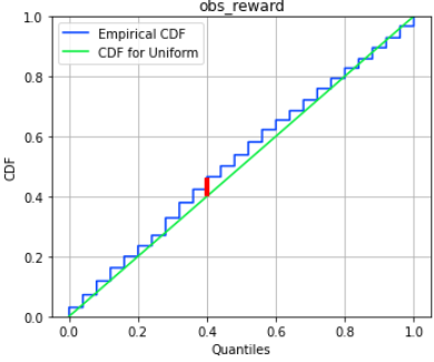
Figure 5: Kolmogorov-Smirnov (KS) statistic (in red) of the predicted reward.

Calibratedness (KS): This metric is computed using the quantile (under the model distribution) of the ground truth values. Hypothetically, these quantiles are uniform if the error we make on the ground truth is a random variable distributed according to a Gaussian having the predicted standard deviation, a property we characterize as calibratedness. To assess this, we compute the Kolmogorov-Smirnov (KS) statistics. Formally, starting from the model cumulative distribution function (CDF) $F_{\theta}(s_{t+1}|s_{t},a_{t})$, we define the empirical CDF of the quantiles of ground truth values by ${\cal F}_{\theta,j}(x)=\frac{\big{|}\big{\{}(s_{t},a_{t},s_{t+1})\in{\cal D}|F^{j}_{\theta}(s_{t+1}|s_{t},a_{t})\leq x\big{\}}\big{|}}{N}$ for $x\in[0,1]$. We denote by $U(x)$ the CDF of the uniform distribution over the interval $[0,1]$, and we define the KS statistics as the largest absolute difference between the two CDFs across the data set ${\cal D}$:

$$\begin{split}\text{KS}({\cal D};\theta;j\in\{1,\ldots,d_{s}\})&=\\ &\max_{i\in\{1,\ldots,N\}}\left|{\cal F}_{\theta,j}(F^{j}_{\theta}(s_{i,t+1}|s_{i,t},a_{i,t}))-U(F^{j}_{\theta}(s_{i,t+1}|s_{i,t},a_{i,t}))\right|\end{split}$$ (5)

The KS score is between zero and one, the lower the better.

Long horizon metrics KS($L$) and R2($L$): Although the models are trained to optimize the one-step prediction log-likelihood score, we want to assess their precision and calibratedness at a longer horizon. Indeed, during the agent learning phase we sample trajectories of multiple steps which can lead to uncertain regions in the case of significant compounding errors down the horizon. For this purpose, we use ground truth actions from a system trace to generate a population of $n\in{\mathbb{N}}$ trajectories of length $L_{\max}$: ${\cal Y}_{L}=[\hat{{\boldsymbol{s}}}_{\ell,t+1:t+L_{\max}}]_{\ell=1}^{n}$ and use the mean predictions to compute a Monte-Carlo estimate of the R2($L$) metric, for $L=0,\ldots,L_{\max}$, using the sample mean $\hat{\mu}_{\theta}(s_{t+L}|s_{t},a_{t})=\frac{1}{n}\sum_{\hat{{\boldsymbol{s}}}\in{\cal Y}_{L}}\hat{s}_{t+L}$ as approximate prediction. For the KS($L$) metric, we estimate the model CDF with the order statistic $F_{\theta}(s_{t+L}|s_{t},a_{t})=\frac{|\{\hat{{\boldsymbol{s}}}\in{\cal Y}_{L}:\hat{s}_{t+L}\leq s_{t+L}\}|}{n}$ among the population of trajectories.

Appendix D Per-dimension static metrics

In all plots, as in Table 1, the KS score is multiplied by 1000, and the OR and R2 scores are multiplied by 10000,

D.1 Random dataset

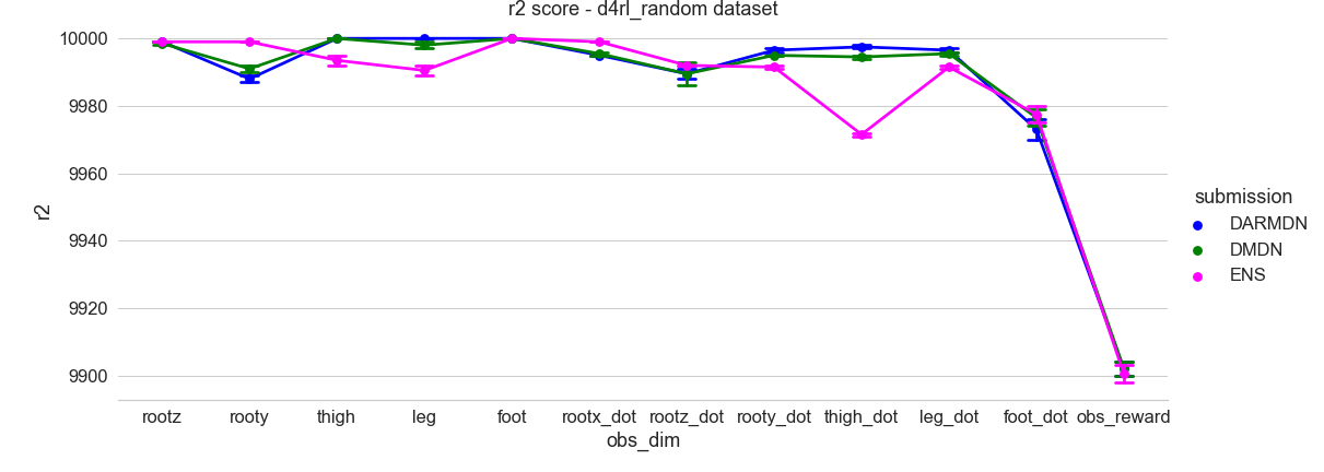
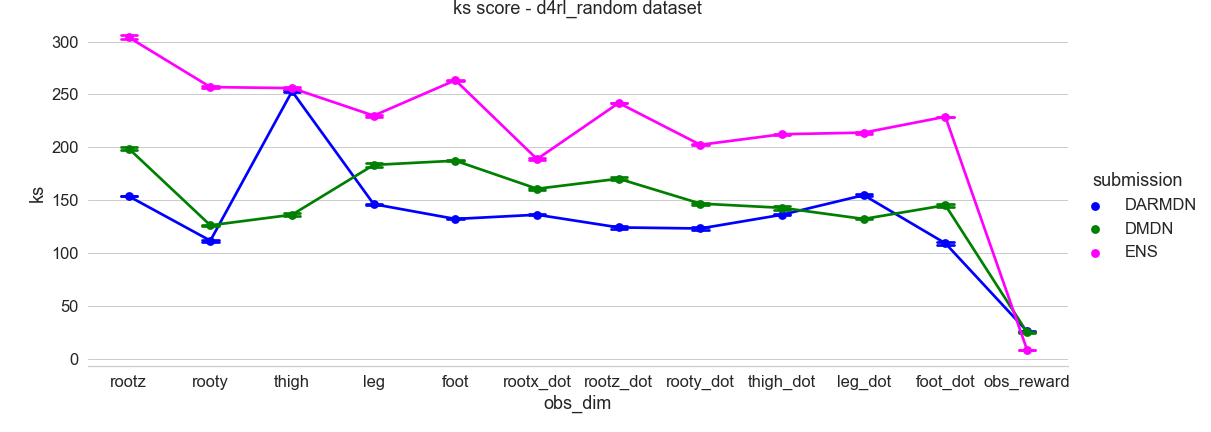
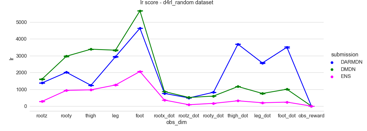
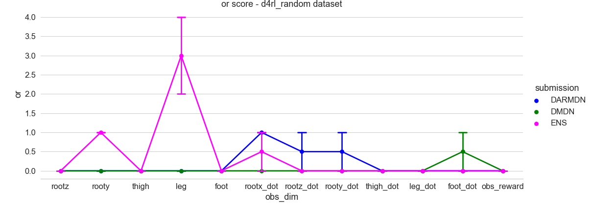
Figure 6: Per-dimension static metrics in the random dataset. The metrics include: R2, KS, LR, and OR. They are computed for all Hopper observables, in addition to the predicted reward (labeled obs_reward). The dots show the mean $\pm$ the standard deviation among the training and the validation scores for each metric.

D.2 Medium dataset

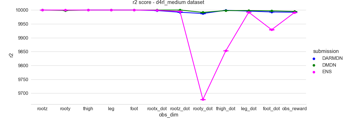
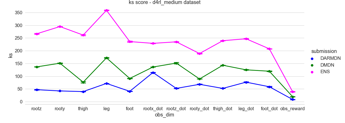
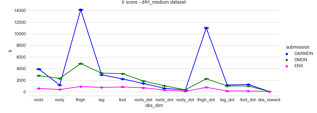
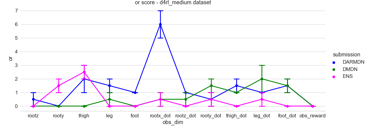
Figure 7: Per-dimension static metrics in the medium dataset. The metrics include: R2, KS, LR, and OR. They are computed for all Hopper observables, in addition to the predicted reward (labeled obs_reward). The dots show the mean $\pm$ the standard deviation among the training and the validation scores for each metric.

D.3 Medium-replay dataset

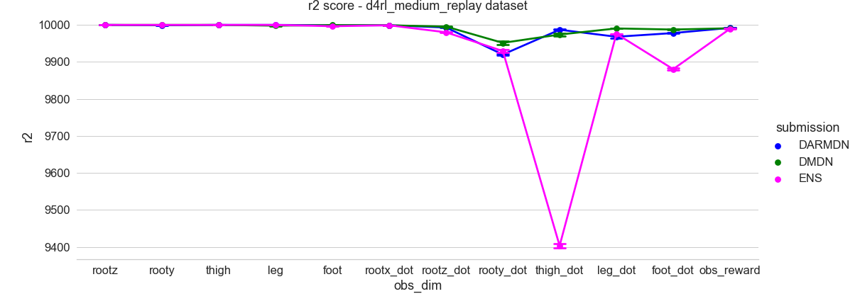
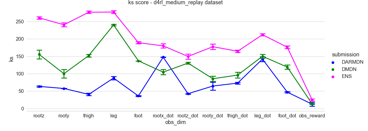
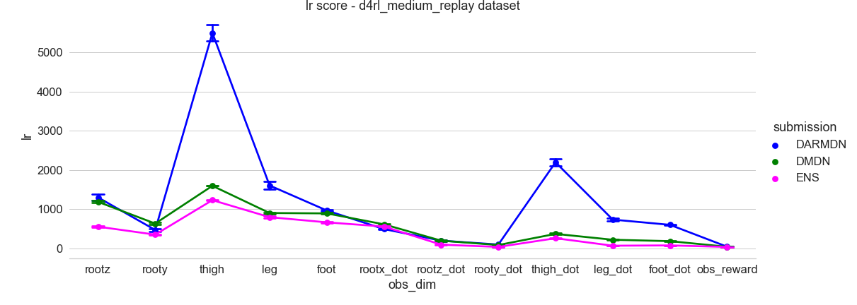
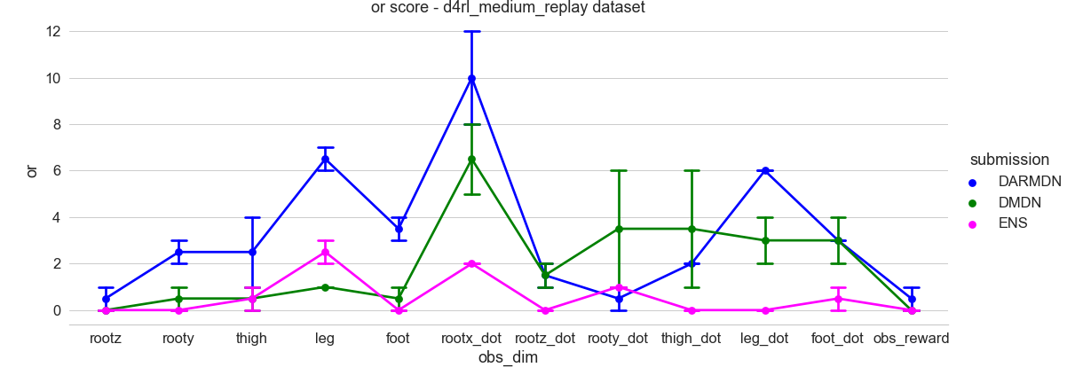
Figure 8: Per-dimension static metrics in the medium-replay dataset. The metrics include: R2, KS, LR, and OR. They and are computed for all Hopper observables, in addition to the predicted reward (labeled obs_reward). The dots show the mean $\pm$ the standard deviation among the training and the validation scores for each metric.

D.4 Medium-expert dataset

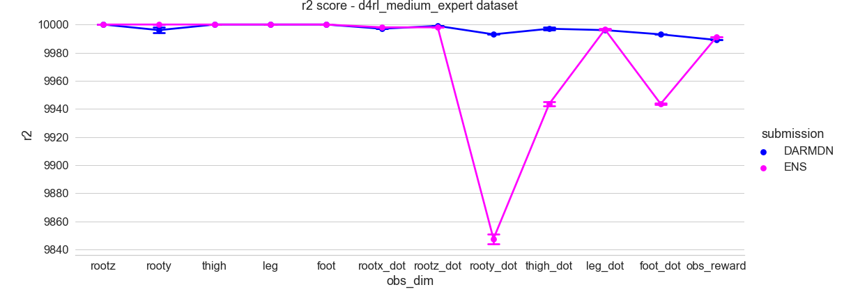
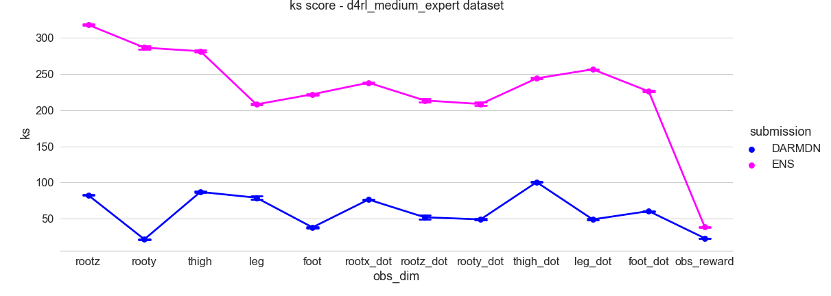
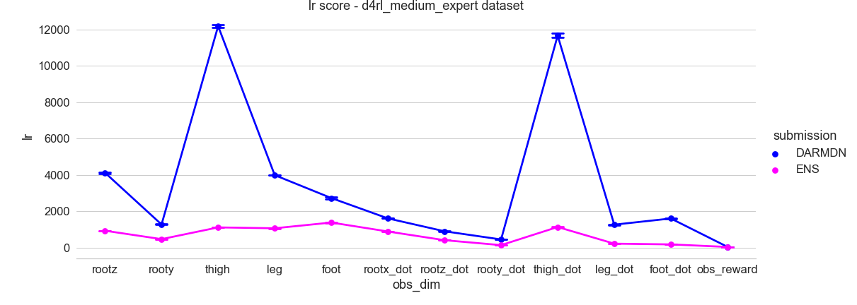
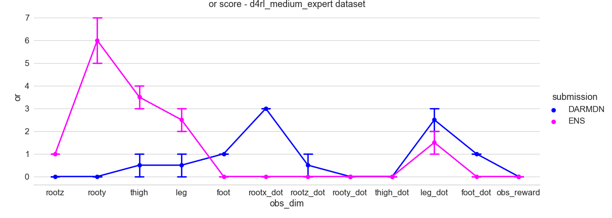
Figure 9: Per-dimension static metrics in the medium-expert dataset. The metrics include: R2, KS, LR, and OR. They are computed for all Hopper observables, in addition to the predicted reward (labeled obs_reward). The dots show the mean $\pm$ the standard deviation among the training and the validation scores for each metric.

Appendix E Error quantile histograms

E.1 Random dataset

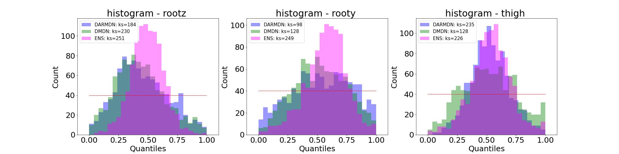
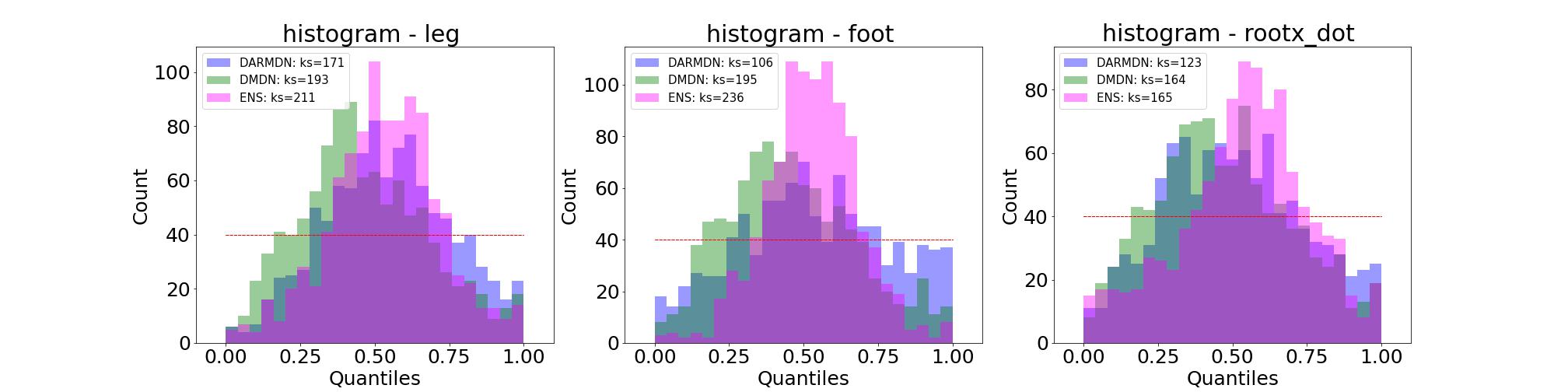
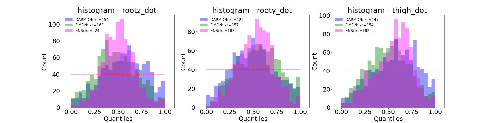
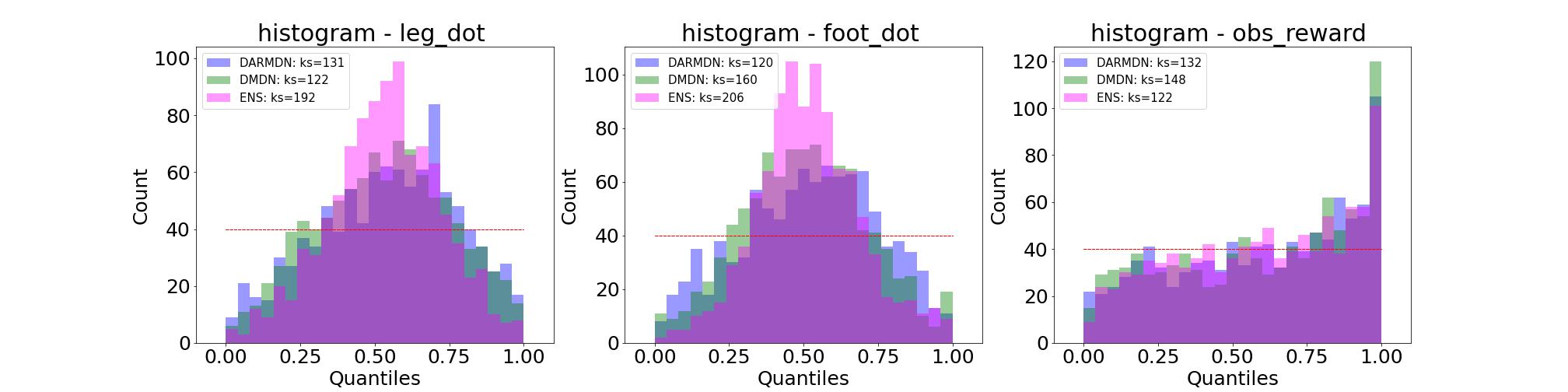
Figure 10: Per-dimension Error quantile histograms in the random dataset. The plot shows the ground truth validation quantiles under the model distribution. The legend includes the value of the KS calibratedness metric, and the dotted red line indicates the ideal case when the quantiles follow a uniform distribution. The histograms are computed for all Hopper observables, in addition to the predicted reward (labeled obs_reward).

E.2 Medium dataset

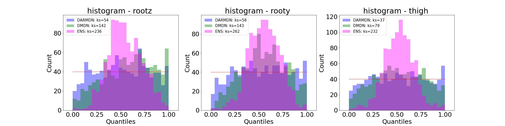
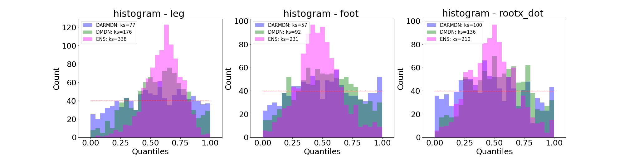
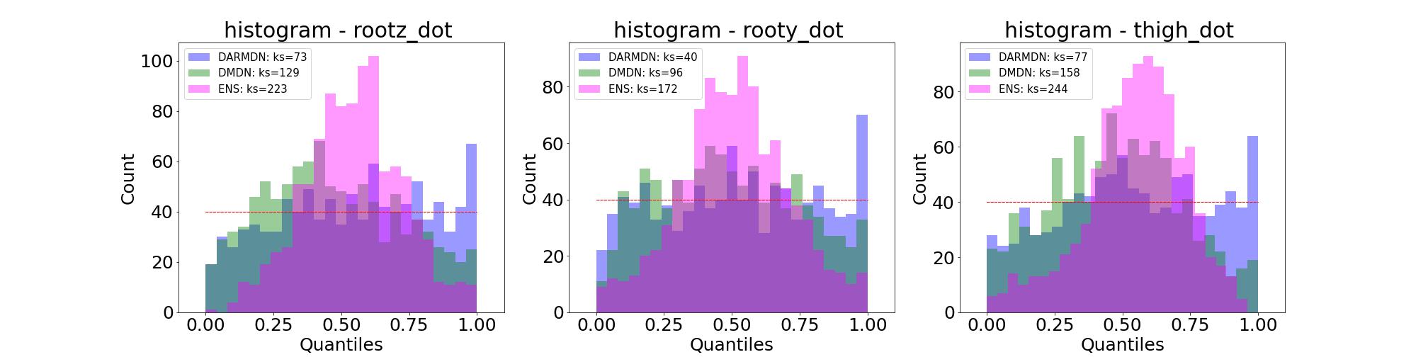
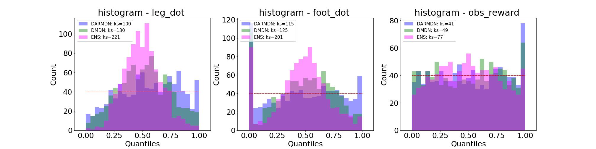
Figure 11: Per-dimension Error quantile histograms in the medium dataset. The plot shows the ground truth validation quantiles under the model distribution. The legend includes the value of the KS calibratedness metric, and the dotted red line indicates the ideal case when the quantiles follow a uniform distribution. The histograms are computed for all Hopper observables, in addition to the predicted reward (labeled obs_reward).

E.3 Medium-replay dataset

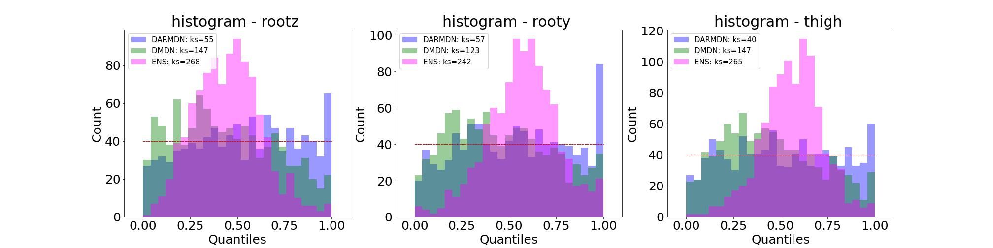
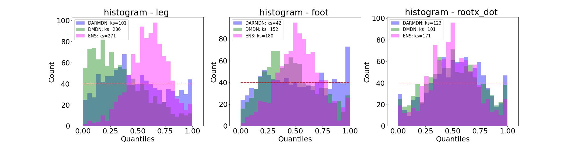
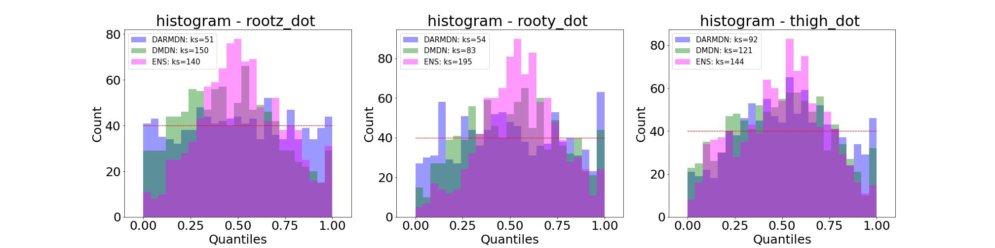
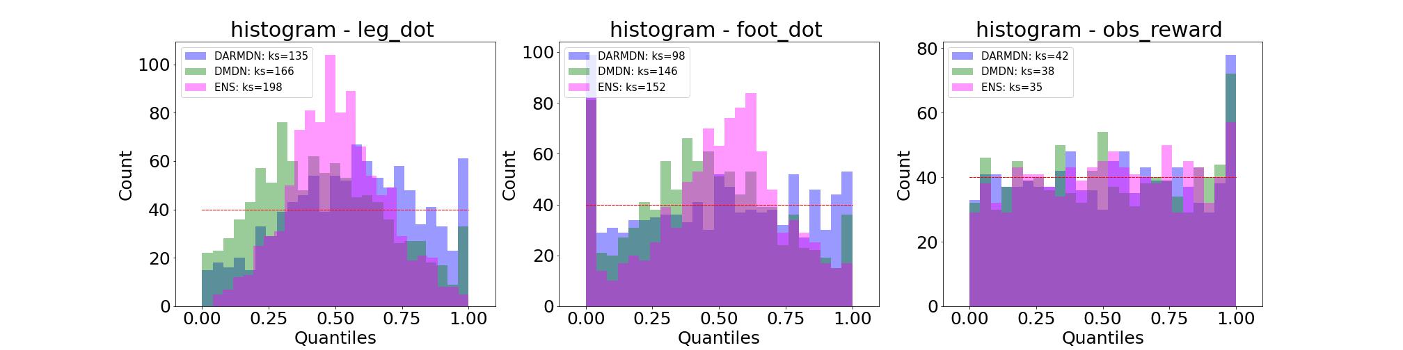
Figure 12: Per-dimension Error quantile histograms in the medium-replay dataset. The plot shows the ground truth validation quantiles under the model distribution. The legend includes the value of the KS calibratedness metric, and the dotted red line indicates the ideal case when the quantiles follow a uniform distribution. The histograms are computed for all Hopper observables, in addition to the predicted reward (labeled obs_reward).

E.4 Medium-expert dataset

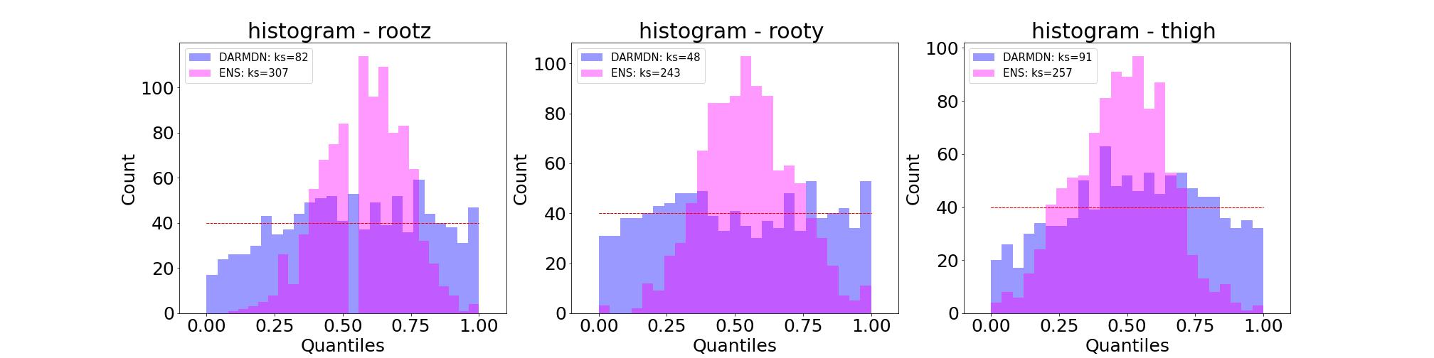
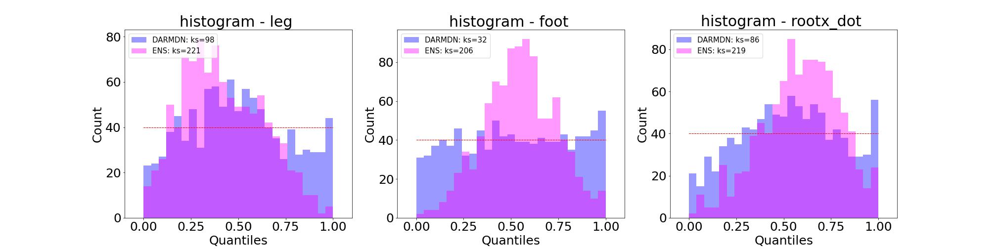
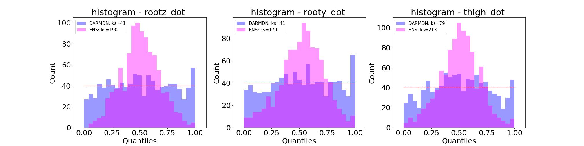
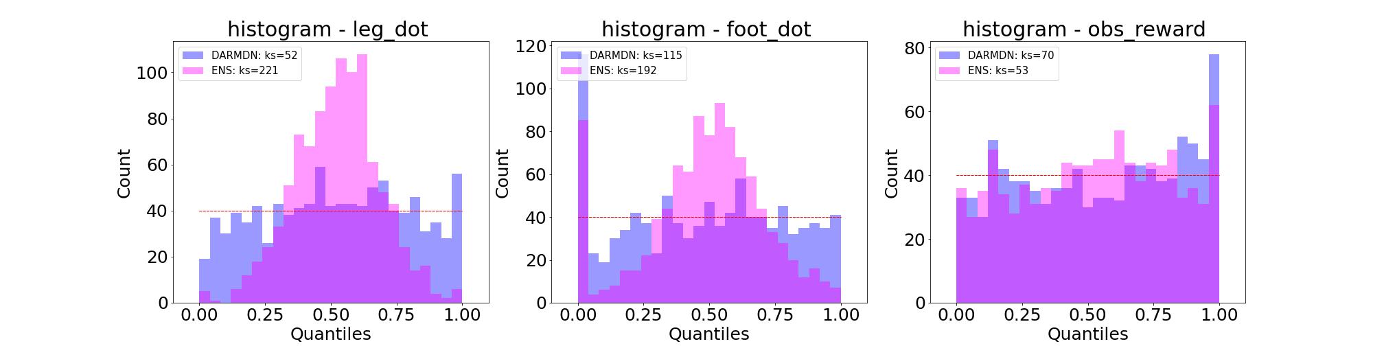
Figure 13: Per-dimension Error quantile histograms in the medium-expert dataset. The plot shows the ground truth validation quantiles under the model distribution. The legend includes the value of the KS calibratedness metric, and the dotted red line indicates the ideal case when the quantiles follow a uniform distribution. The histograms are computed for all Hopper observables, in addition to the predicted reward (labeled obs_reward).

Appendix F Long horizon metrics

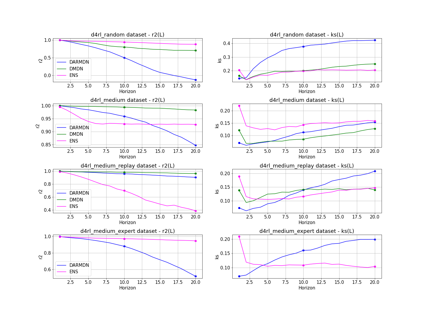
Figure 14: Long horizon explained variance R2($L$) and calibratedness KS($L$). The metric is aggregated by averaging over Hopper’s observables and predicted reward.

Appendix G Static and dynamic metrics correlations

G.1 Random dataset

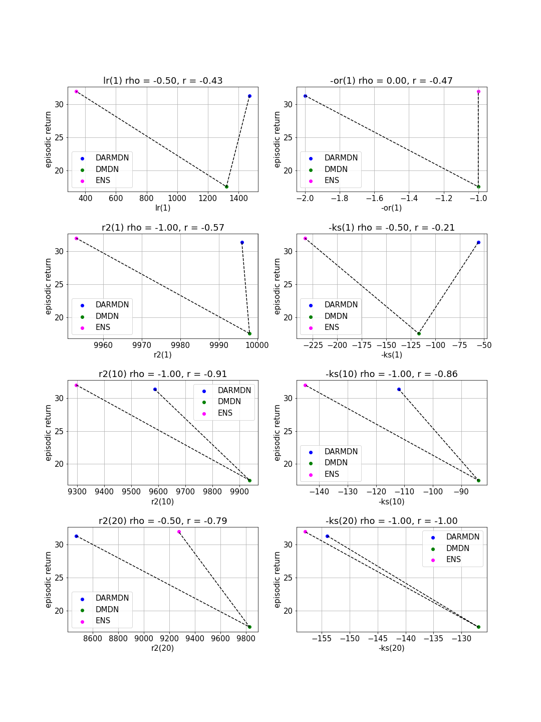
Figure 15: The Spearman and Pearson correlations between the episodic return and the static metrics (LR, negative OR, R2($1$), negative KS($1$), R2($10$), negative KS($10$), R2($20$), negative KS($20$)) in the random dataset. To uniformly evaluate the metrics’ positive correlation with the episodic return, we take the negative of the metrics where the smaller is the better (KS($L$) and OR).

G.2 Medium dataset

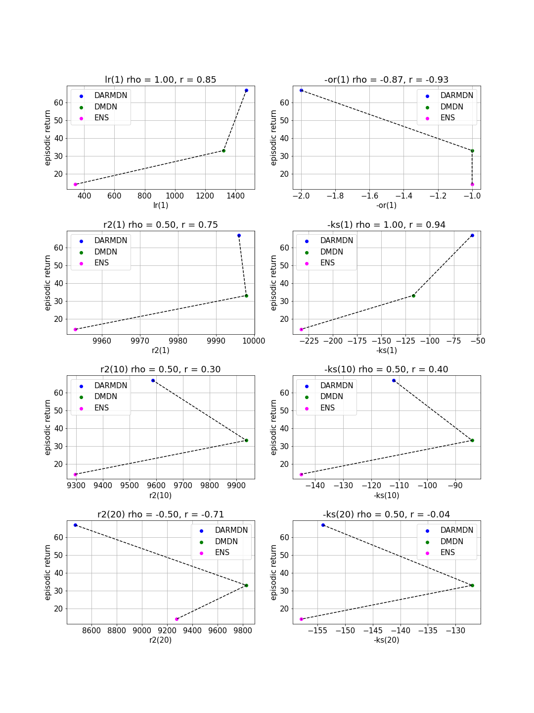
Figure 16: The Spearman and Pearson correlations between the episodic return and the static metrics (LR, negative OR, R2($1$), negative KS($1$), R2($10$), negative KS($10$), R2($20$), negative KS($20$)) in the medium dataset. To uniformly evaluate the metrics’ positive correlation with the episodic return, we take the negative of the metrics where the smaller is the better (KS($L$) and OR).

G.3 Medium-replay dataset

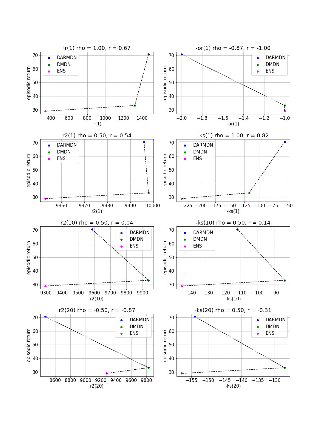
Figure 17: The Spearman and Pearson correlations between the episodic return and the static metrics (LR, negative OR, R2($1$), negative KS($1$), R2($10$), negative KS($10$), R2($20$), negative KS($20$)) in the medium-replay dataset. To uniformly evaluate the metrics’ positive correlation with the episodic return, we take the negative of the metrics where the smaller is the better (KS($L$) and OR).

G.4 Medium-expert dataset

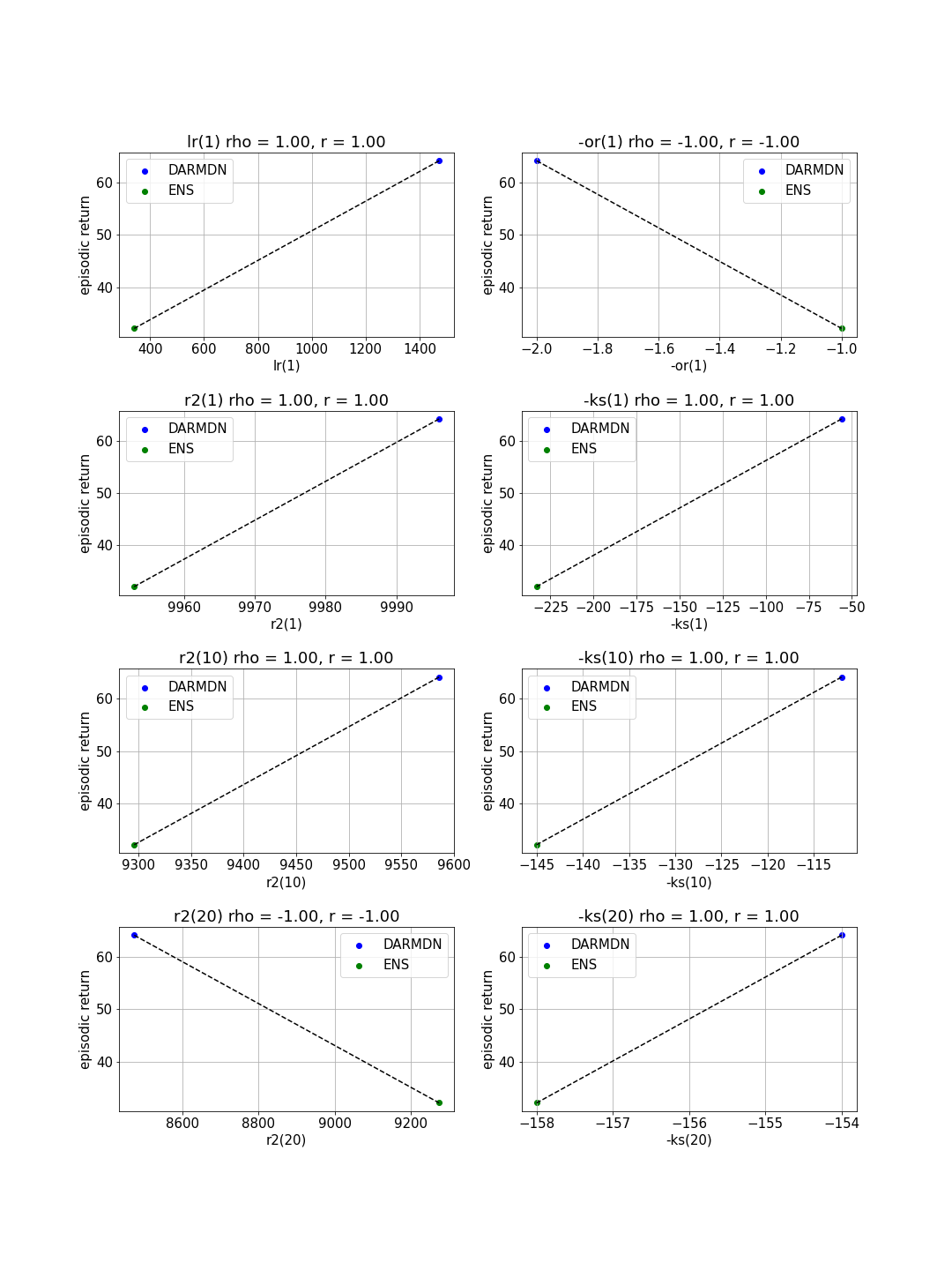
Figure 18: The Spearman and Pearson correlations between the episodic return and the static metrics (LR, negative OR, R2($1$), negative KS($1$), R2($10$), negative KS($10$), R2($20$), negative KS($20$)) in the medium-expert dataset. To uniformly evaluate the metrics’ positive correlation with the episodic return, we take the negative of the metrics where the smaller is the better (KS($L$) and OR).

References

- Andrychowicz et al. (2021) Marcin Andrychowicz, Anton Raichuk, Piotr Stańczyk, Manu Orsini, Sertan Girgin, Raphaël Marinier, Leonard Hussenot, Matthieu Geist, Olivier Pietquin, Marcin Michalski, Sylvain Gelly, and Olivier Bachem. What matters for on-policy deep actor-critic methods? a large-scale study. In International Conference on Learning Representations, 2021.
- Argenson & Dulac-Arnold (2021) Arthur Argenson and Gabriel Dulac-Arnold. Model-based offline planning. In International Conference on Learning Representations, 2021.
- Brockman et al. (2016) Greg Brockman, Vicki Cheung, Ludwig Pettersson, Jonas Schneider, John Schulman, Jie Tang, and Wojciech Zaremba. OpenAI gym, 2016.
- Chebotar et al. (2021) Yevgen Chebotar, Karol Hausman, Yao Lu, Ted Xiao, Dmitry Kalashnikov, Jake Varley, Alex Irpan, Benjamin Eysenbach, Ryan Julian, Chelsea Finn, and Sergey Levine. Actionable models: Unsupervised offline reinforcement learning of robotic skills. CoRR, abs/2104.07749, 2021. URL https://arxiv.org/abs/2104.07749.
- Chua et al. (2018) Kurtland Chua, Roberto Calandra, Rowan McAllister, and Sergey Levine. Deep reinforcement learning in a handful of trials using probabilistic dynamics models. In Advances in Neural Information Processing Systems 31, pp. 4754–4765. Curran Associates, Inc., 2018.
- Degris et al. (2012) Thomas Degris, Martha White, and Richard S. Sutton. Off-policy actor-critic. In Proceedings of the 29th International Conference on Machine Learning, ICML’12, pp. 179–186, Madison, WI, USA, 2012. Omnipress. ISBN 9781450312851.
- Deisenroth & Rasmussen (2011) Marc Peter Deisenroth and Carl Edward Rasmussen. PILCO: A model-based and data-efficient approach to policy search. In Proceedings of the International Conference on Machine Learning, 2011.
- Depeweg et al. (2018) Stefan Depeweg, José Miguel Hernández-Lobato, Finale Doshi-Velez, and Steffen Udluft. Decomposition of uncertainty in bayesian deep learning for efficient and risk-sensitive learning. In ICML, 2018.
- Draeger et al. (1995) Andreas Draeger, Sebastian Engell, and Horst Ranke. Model predictive control using neural networks. IEEE Control Systems, 15:61–66, 1995. ISSN 1066033X. doi: 10.1109/37.466261.
- Engstrom et al. (2020) Logan Engstrom, Andrew Ilyas, Shibani Santurkar, Dimitris Tsipras, Firdaus Janoos, Larry Rudolph, and Aleksander Madry. Implementation matters in deep rl: A case study on ppo and trpo. In International Conference on Learning Representations, 2020. URL https://openreview.net/forum?id=r1etN1rtPB.
- Fu et al. (2021a) Justin Fu, Aviral Kumar, Ofir Nachum, George Tucker, and Sergey Levine. D4rl: Datasets for deep data-driven reinforcement learning, 2021a. URL https://openreview.net/forum?id=px0-N3_KjA.
- Fu et al. (2021b) Justin Fu, Mohammad Norouzi, Ofir Nachum, George Tucker, Ziyu Wang, Alexander Novikov, Mengjiao Yang, Michael R. Zhang, Yutian Chen, Aviral Kumar, Cosmin Paduraru, Sergey Levine, and Tom Le Paine. Benchmarks for deep off-policy evaluation, 2021b.
- Fujimoto et al. (2019) Scott Fujimoto, David Meger, and Doina Precup. Off-policy deep reinforcement learning without exploration. In Kamalika Chaudhuri and Ruslan Salakhutdinov (eds.), Proceedings of the 36th International Conference on Machine Learning, volume 97 of Proceedings of Machine Learning Research, pp. 2052–2062. PMLR, 09–15 Jun 2019. URL https://proceedings.mlr.press/v97/fujimoto19a.html.
- Gal et al. (2016) Yarin Gal, Rowan McAllister, and Carl Edward Rasmussen. Improving PILCO with Bayesian neural network dynamics models. In Data-Efficient Machine Learning workshop, International Conference on Machine Learning, 2016.
- Gottesman et al. (2018) Omer Gottesman, Fredrik D. Johansson, Joshua Meier, Jack Dent, Donghun Lee, Srivatsan Srinivasan, Linying Zhang, Yi Ding, David Wihl, Xuefeng Peng, Jiayu Yao, Isaac Lage, Christopher Mosch, Li wei H. Lehman, Matthieu Komorowski, A. Aldo Faisal, Leo Anthony Celi, David A. Sontag, and Finale Doshi-Velez. Evaluating reinforcement learning algorithms in observational health settings. ArXiv, abs/1805.12298, 2018.
- Ha & Schmidhuber (2018) David Ha and Jürgen Schmidhuber. Recurrent world models facilitate policy evolution. In S. Bengio, H. Wallach, H. Larochelle, K. Grauman, N. Cesa-Bianchi, and R. Garnett (eds.), Advances in Neural Information Processing Systems 31, pp. 2450–2462. Curran Associates, Inc., 2018.
- Haarnoja et al. (2018) Tuomas Haarnoja, Aurick Zhou, Pieter Abbeel, and Sergey Levine. Soft Actor-Critic: Off-Policy Maximum Entropy Deep Reinforcement Learning with a Stochastic Actor. In Jennifer Dy and Andreas Krause (eds.), Proceedings of the 35th International Conference on Machine Learning, volume 80 of Proceedings of Machine Learning Research, pp. 1861–1870. PMLR, 10–15 Jul 2018.
- Hafner et al. (2019) Danijar Hafner, Timothy Lillicrap, Ian Fischer, Ruben Villegas, David Ha, Honglak Lee, and James Davidson. Learning latent dynamics for planning from pixels. In Proceedings of the 36th International Conference on Machine Learning, volume 97 of Proceedings of Machine Learning Research, pp. 2555–2565, 2019.
- Hafner et al. (2021) Danijar Hafner, Timothy P Lillicrap, Mohammad Norouzi, and Jimmy Ba. Mastering atari with discrete world models. In International Conference on Learning Representations, 2021. URL https://openreview.net/forum?id=0oabwyZbOu.
- Hüllermeier & Waegeman (2021) Eyke Hüllermeier and Willem Waegeman. Aleatoric and epistemic uncertainty in machine learning: An introduction to concepts and methods. Machine Learning, 110(3):457–506, 2021.
- Ioffe & Szegedy (2015) Sergey Ioffe and Christian Szegedy. Batch normalization: Accelerating deep network training by reducing internal covariate shift. In Proceedings of the 32nd International Conference on International Conference on Machine Learning - Volume 37, ICML’15, pp. 448–456. JMLR.org, 2015.
- Janner et al. (2019) Michael Janner, Justin Fu, Marvin Zhang, and Sergey Levine. When to trust your model: Model-based policy optimization. In H. Wallach, H. Larochelle, A. Beygelzimer, F. d'Alché-Buc, E. Fox, and R. Garnett (eds.), Advances in Neural Information Processing Systems, volume 32. Curran Associates, Inc., 2019.
- Kégl et al. (2018) Balázs Kégl, Alexandre Boucaud, Mehdi Cherti, Akin Kazakci, Alexandre Gramfort, Guillaume Lemaitre, Joris Van den Bossche, Djalel Benbouzid, and Camille Marini. The RAMP framework: from reproducibility to transparency in the design and optimization of scientific workflows. In ICML workshop on Reproducibility in Machine Learning, 2018.
- Kégl et al. (2021) Balázs Kégl, Gabriel Hurtado, and Albert Thomas. Model-based micro-data reinforcement learning: what are the crucial model properties and which model to choose? In International Conference on Learning Representations, 2021. URL https://openreview.net/forum?id=p5uylG94S68.
- Kidambi et al. (2020) Rahul Kidambi, Aravind Rajeswaran, Praneeth Netrapalli, and Thorsten Joachims. Morel: Model-based offline reinforcement learning. In H. Larochelle, M. Ranzato, R. Hadsell, M.F. Balcan, and H. Lin (eds.), Advances in Neural Information Processing Systems, volume 33, pp. 21810–21823. Curran Associates, Inc., 2020. URL https://proceedings.neurips.cc/paper/2020/file/f7efa4f864ae9b88d43527f4b14f750f-Paper.pdf.
- Kingma & Ba (2015) Diederik P. Kingma and Jimmy Ba. Adam: A method for stochastic optimization. In Yoshua Bengio and Yann LeCun (eds.), 3rd International Conference on Learning Representations, ICLR 2015, San Diego, CA, USA, May 7-9, 2015, Conference Track Proceedings, 2015. URL http://arxiv.org/abs/1412.6980.
- Kiran et al. (2022) B Ravi Kiran, Ibrahim Sobh, Victor Talpaert, Patrick Mannion, Ahmad A. Al Sallab, Senthil Yogamani, and Patrick Pérez. Deep reinforcement learning for autonomous driving: A survey. IEEE Transactions on Intelligent Transportation Systems, 23(6):4909–4926, 2022. doi: 10.1109/TITS.2021.3054625.
- Kumar et al. (2019) Aviral Kumar, Justin Fu, Matthew Soh, George Tucker, and Sergey Levine. Stabilizing off-policy q-learning via bootstrapping error reduction. In H. Wallach, H. Larochelle, A. Beygelzimer, F. d'Alché-Buc, E. Fox, and R. Garnett (eds.), Advances in Neural Information Processing Systems, volume 32. Curran Associates, Inc., 2019. URL https://proceedings.neurips.cc/paper/2019/file/c2073ffa77b5357a498057413bb09d3a-Paper.pdf.
- Kumar et al. (2020) Aviral Kumar, Aurick Zhou, George Tucker, and Sergey Levine. Conservative q-learning for offline reinforcement learning. In Proceedings of the 34th International Conference on Neural Information Processing Systems, NIPS’20, Red Hook, NY, USA, 2020. Curran Associates Inc. ISBN 9781713829546.
- Lakshminarayanan et al. (2017) Balaji Lakshminarayanan, Alexander Pritzel, and Charles Blundell. Simple and scalable predictive uncertainty estimation using deep ensembles. In Proceedings of the 31st International Conference on Neural Information Processing Systems, NIPS’17, pp. 6405–6416, Red Hook, NY, USA, 2017. Curran Associates Inc. ISBN 9781510860964.
- Lee et al. (2021) Byung-Jun Lee, Jongmin Lee, and Kee-Eung Kim. Representation balancing offline model-based reinforcement learning. In International Conference on Learning Representations, 2021. URL https://openreview.net/forum?id=QpNz8r_Ri2Y.
- Levine & Koltun (2013) Sergey Levine and Vladlen Koltun. Guided policy search. In Sanjoy Dasgupta and David McAllester (eds.), Proceedings of the 30th International Conference on Machine Learning, volume 28 of Proceedings of Machine Learning Research, pp. 1–9, Atlanta, Georgia, USA, 17–19 Jun 2013. PMLR. URL https://proceedings.mlr.press/v28/levine13.html.
- Levine et al. (2020) Sergey Levine, Aviral Kumar, George Tucker, and Justin Fu. Offline reinforcement learning: Tutorial, review, and perspectives on open problems. arXiv preprint arXiv:2005.01643, 2020.
- Lillicrap et al. (2016) Timothy P. Lillicrap, Jonathan J. Hunt, Alexander Pritzel, Nicolas Heess, Tom Erez, Yuval Tassa, David Silver, and Daan Wierstra. Continuous control with deep reinforcement learning. In ICLR (Poster), 2016. URL http://arxiv.org/abs/1509.02971.
- Liu et al. (2021) Ruizhen Liu, Zhicong Chen, and Dazhi Zhong. Dromo: Distributionally robust offline model-based policy optimization. 2021.
- Lu et al. (2022) Cong Lu, Philip Ball, Jack Parker-Holder, Michael Osborne, and Stephen J. Roberts. Revisiting design choices in offline model based reinforcement learning. In International Conference on Learning Representations, 2022. URL https://openreview.net/forum?id=zz9hXVhf40.
- Matsushima et al. (2021) Tatsuya Matsushima, Hiroki Furuta, Yutaka Matsuo, Ofir Nachum, and Shixiang Gu. Deployment-efficient reinforcement learning via model-based offline optimization. In International Conference on Learning Representations, 2021.
- Mnih et al. (2015) Volodymyr Mnih, Koray Kavukcuoglu, David Silver, Andrei A. Rusu, Joel Veness, Marc G. Bellemare, Alex Graves, Martin Riedmiller, Andreas K. Fidjeland, Georg Ostrovski, Stig Petersen, Charles Beattie, Amir Sadik, Ioannis Antonoglou, Helen King, Dharshan Kumaran, Daan Wierstra, Shane Legg, and Demis Hassabis. Human-level control through deep reinforcement learning. Nature, 518(7540):529–533, 2015.
- Moritz et al. (2018) Philipp Moritz, Robert Nishihara, Stephanie Wang, Alexey Tumanov, Richard Liaw, Eric Liang, Melih Elibol, Zongheng Yang, William Paul, Michael I. Jordan, and Ion Stoica. Ray: A distributed framework for emerging ai applications. In Proceedings of the 13th USENIX Conference on Operating Systems Design and Implementation, OSDI’18, pp. 561–577, USA, 2018. USENIX Association. ISBN 9781931971478.
- Munos et al. (2016) Rémi Munos, Thomas Stepleton, Anna Harutyunyan, and Marc G. Bellemare. Safe and efficient off-policy reinforcement learning. In Proceedings of the 30th International Conference on Neural Information Processing Systems, NIPS’16, pp. 1054–1062, Red Hook, NY, USA, 2016. Curran Associates Inc. ISBN 9781510838819.
- Nachum et al. (2019) Ofir Nachum, Bo Dai, Ilya Kostrikov, Yinlam Chow, Lihong Li, and Dale Schuurmans. Algaedice: Policy gradient from arbitrary experience. CoRR, abs/1912.02074, 2019. URL http://arxiv.org/abs/1912.02074.
- Nagabandi et al. (2018) Anusha Nagabandi, Gregory Kahn, Ronald S. Fearing, and Sergey Levine. Neural network dynamics for model-based deep reinforcement learning with model-free fine-tuning. In 2018 IEEE International Conference on Robotics and Automation, ICRA 2018, pp. 7559–7566. IEEE, 2018.
- Osband et al. (2021) Ian Osband, Zheng Wen, Seyed Mohammad Asghari, Vikranth Dwaracherla, Morteza Ibrahimi, Xiuyuan Lu, and Benjamin Van Roy. Epistemic neural networks, 2021. URL https://arxiv.org/abs/2107.08924.
- Paine et al. (2020) Tom Le Paine, Cosmin Paduraru, Andrea Michi, Çaglar Gülçehre, Konrad Zolna, Alexander Novikov, Ziyu Wang, and Nando de Freitas. Hyperparameter selection for offline reinforcement learning. CoRR, abs/2007.09055, 2020. URL https://arxiv.org/abs/2007.09055.
- Papamakarios et al. (2017) George Papamakarios, Theo Pavlakou, and Iain Murray. Masked autoregressive flow for density estimation. In Proceedings of the 31st International Conference on Neural Information Processing Systems, NIPS’17, pp. 2335–2344, Red Hook, NY, USA, 2017. Curran Associates Inc. ISBN 9781510860964.
- Peng et al. (2020) Xue Bin Peng, Aviral Kumar, Grace Zhang, and Sergey Levine. Advantage weighted regression: Simple and scalable off-policy reinforcement learning, 2020. URL https://openreview.net/forum?id=H1gdF34FvS.
- Pineda et al. (2021) Luis Pineda, Brandon Amos, Amy Zhang, Nathan O. Lambert, and Roberto Calandra. Mbrl-lib: A modular library for model-based reinforcement learning. Arxiv, 2021. URL https://arxiv.org/abs/2104.10159.
- Pinneri et al. (2020) Cristina Pinneri, Shambhuraj Sawant, Sebastian Blaes, Jan Achterhold, Joerg Stueckler, Michal Rolinek, and Georg Martius. Sample-efficient cross-entropy method for real-time planning. In Conference on Robot Learning 2020, 2020. URL https://corlconf.github.io/corl2020/paper_217/.
- Raffin et al. (2021) Antonin Raffin, Ashley Hill, Adam Gleave, Anssi Kanervisto, Maximilian Ernestus, and Noah Dormann. Stable-baselines3: Reliable reinforcement learning implementations. Journal of Machine Learning Research, 22(268):1–8, 2021. URL http://jmlr.org/papers/v22/20-1364.html.
- Shen et al. (2021) Jian Shen, Mingcheng Chen, Zhicheng Zhang, Zhengyu Yang, Weinan Zhang, and Yong Yu. Model-based offline policy optimization with distribution correcting regularization. volume 12975 LNAI, pp. 174–189. Springer Science and Business Media Deutschland GmbH, 2021. ISBN 9783030864859. doi: 10.1007/978-3-030-86486-6˙11.
- Silver et al. (2017) David Silver, Thomas Hubert, Julian Schrittwieser, Ioannis Antonoglou, Matthew Lai, Arthur Guez, Marc Lanctot, Laurent Sifre, Dharshan Kumaran, Thore Graepel, Timothy Lillicrap, Karen Simonyan, and Demis Hassabis. Mastering chess and shogi by self-play with a general reinforcement learning algorithm, 2017.
- Silver et al. (2018) David Silver, Thomas Hubert, Julian Schrittwieser, Ioannis Antonoglou, Matthew Lai, Arthur Guez, Marc Lanctot, Laurent Sifre, Dharshan Kumaran, Thore Graepel, Timothy Lillicrap, Karen Simonyan, and Demis Hassabis. A general reinforcement learning algorithm that masters Chess, Shogi, and Go through self-play. Science, 362(6419):1140–1144, 2018. ISSN 0036-8075. doi: 10.1126/science.aar6404.
- Srivastava et al. (2014) Nitish Srivastava, Geoffrey Hinton, Alex Krizhevsky, Ilya Sutskever, and Ruslan Salakhutdinov. Dropout: A simple way to prevent neural networks from overfitting. Journal of Machine Learning Research, 15(56):1929–1958, 2014. URL http://jmlr.org/papers/v15/srivastava14a.html.
- Strehl et al. (2010) Alexander L. Strehl, John Langford, Lihong Li, and Sham M. Kakade. Learning from logged implicit exploration data. In Proceedings of the 23rd International Conference on Neural Information Processing Systems - Volume 2, NIPS’10, pp. 2217–2225, Red Hook, NY, USA, 2010. Curran Associates Inc.
- Sutton (1991) Richard S. Sutton. Dyna, an integrated architecture for learning, planning, and reacting. ACM SIGART Bulletin, 2:160–163, 7 1991. ISSN 0163-5719. doi: 10.1145/122344.122377. URL https://dl.acm.org/doi/10.1145/122344.122377.
- Sutton et al. (1992) Richard S Sutton, Csaba Szepesvári, Alborz Geramifard, and Michael Bowling. Dyna-style planning with linear function approximation and prioritized sweeping. Moore and Atkeson, 1992.
- Swazinna et al. (2021) Phillip Swazinna, Steffen Udluft, and Thomas Runkler. Overcoming model bias for robust offline deep reinforcement learning. Engineering Applications of Artificial Intelligence, 104:104366, 2021. ISSN 0952-1976. doi: https://doi.org/10.1016/j.engappai.2021.104366. URL https://www.sciencedirect.com/science/article/pii/S0952197621002141.
- Todorov et al. (2012) Emanuel Todorov, Tom Erez, and Yuval Tassa. Mujoco: A physics engine for model-based control. In 2012 IEEE/RSJ International Conference on Intelligent Robots and Systems, pp. 5026–5033, 2012. doi: 10.1109/IROS.2012.6386109.
- Uria et al. (2013) Benigno Uria, Iain Murray, and Hugo Larochelle. RNADE: The real-valued neural autoregressive density-estimator. In Advances in Neural Information Processing Systems 26, pp. 2175–2183. Curran Associates Inc., 2013.
- Uria et al. (2016) Benigno Uria, Marc-Alexandre Côté, Karol Gregor, Iain Murray, and Hugo Larochelle. Neural autoregressive distribution estimation. J. Mach. Learn. Res., 17(1):7184–7220, jan 2016. ISSN 1532-4435.
- Van Den Oord et al. (2016) Aäron Van Den Oord, Nal Kalchbrenner, and Koray Kavukcuoglu. Pixel recurrent neural networks. In Proceedings of the 33rd International Conference on International Conference on Machine Learning - Volume 48, ICML’16, pp. 1747–1756. JMLR.org, 2016.
- Vinyals et al. (2019) Oriol Vinyals, Igor Babuschkin, Wojciech M. Czarnecki, Michaël Mathieu, Andrew Dudzik, Junyoung Chung, David H. Choi, Richard Powell, Timo Ewalds, Petko Georgiev, Junhyuk Oh, Dan Horgan, Manuel Kroiss, Ivo Danihelka, Aja Huang, L. Sifre, Trevor Cai, John P. Agapiou, Max Jaderberg, Alexander Sasha Vezhnevets, Rémi Leblond, Tobias Pohlen, Valentin Dalibard, David Budden, Yury Sulsky, James Molloy, Tom Le Paine, Caglar Gulcehre, Ziyun Wang, Tobias Pfaff, Yuhuai Wu, Roman Ring, Dani Yogatama, Dario Wünsch, Katrina McKinney, Oliver Smith, Tom Schaul, Timothy P. Lillicrap, Koray Kavukcuoglu, Demis Hassabis, Chris Apps, and David Silver. Grandmaster level in starcraft ii using multi-agent reinforcement learning. Nature, pp. 1–5, 2019.
- Wang & Ba (2020) Tingwu Wang and Jimmy Ba. Exploring model-based planning with policy networks. In 8th International Conference on Learning Representations, ICLR 2020, 2020.
- Wang et al. (2019) Tingwu Wang, Xuchan Bao, Ignasi Clavera, Jerrick Hoang, Yeming Wen, Eric Langlois, Shunshi Zhang, Guodong Zhang, Pieter Abbeel, and Jimmy Ba. Benchmarking model-based reinforcement learning. arXiv preprint arXiv:1907.02057, 2019.
- Wu et al. (2020) Yifan Wu, George Tucker, and Ofir Nachum. Behavior regularized offline reinforcement learning, 2020. URL https://openreview.net/forum?id=BJg9hTNKPH.
- Yu et al. (2020) Tianhe Yu, Garrett Thomas, Lantao Yu, Stefano Ermon, James Y Zou, Sergey Levine, Chelsea Finn, and Tengyu Ma. Mopo: Model-based offline policy optimization. In H. Larochelle, M. Ranzato, R. Hadsell, M.F. Balcan, and H. Lin (eds.), Advances in Neural Information Processing Systems, volume 33, pp. 14129–14142. Curran Associates, Inc., 2020. URL https://proceedings.neurips.cc/paper/2020/file/a322852ce0df73e204b7e67cbbef0d0a-Paper.pdf.
- Yu et al. (2021) Tianhe Yu, Aviral Kumar, Rafael Rafailov, Aravind Rajeswaran, Sergey Levine, and Chelsea Finn. Combo: Conservative offline model-based policy optimization. In M. Ranzato, A. Beygelzimer, Y. Dauphin, P.S. Liang, and J. Wortman Vaughan (eds.), Advances in Neural Information Processing Systems, volume 34, pp. 28954–28967. Curran Associates, Inc., 2021. URL https://proceedings.neurips.cc/paper/2021/file/f29a179746902e331572c483c45e5086-Paper.pdf.
- Zhan et al. (2021) Xianyuan Zhan, Xiangyu Zhu, and Haoran Xu. Model-based offline planning with trajectory pruning. 2021.
- Zhang et al. (2021a) Bangnig Zhang, Raghunandan Rajan, Luis Pineda, Nathan Lambert, André Biedenkapp, Kurtland Chua, Frank Hutter, and Roberto Calandra. On the importance of hyperparameter optimization for model-based reinforcement learning. In AISTATS, 2021a.
- Zhang et al. (2021b) Michael R Zhang, Thomas Paine, Ofir Nachum, Cosmin Paduraru, George Tucker, ziyu wang, and Mohammad Norouzi. Autoregressive dynamics models for offline policy evaluation and optimization. In International Conference on Learning Representations, 2021b. URL https://openreview.net/forum?id=kmqjgSNXby.