Non-asymptotic Analysis of Biased Adaptive Stochastic Approximation

Sobihan Surendran111Laboratoire de Probabilités, Statistique et Modélisation (LPSM), Sorbonne Université, 75005 Paris, France. 222LOPF, Califrais’ Machine Learning Lab, Paris, France, Adeline Fermanian22footnotemark: 2, Antoine Godichon-Baggioni11footnotemark: 1, and Sylvain Le Corff11footnotemark: 1
Abstract

Stochastic Gradient Descent (SGD) with adaptive steps is now widely used for training deep neural networks. Most theoretical results assume access to unbiased gradient estimators, which is not the case in several recent deep learning and reinforcement learning applications that use Monte Carlo methods. This paper provides a comprehensive non-asymptotic analysis of SGD with biased gradients and adaptive steps for convex and non-convex smooth functions. Our study incorporates time-dependent bias and emphasizes the importance of controlling the bias and Mean Squared Error (MSE) of the gradient estimator. In particular, we establish that Adagrad and RMSProp with biased gradients converge to critical points for smooth non-convex functions at a rate similar to existing results in the literature for the unbiased case. Finally, we provide experimental results using Variational Autoenconders (VAE) that illustrate our convergence results and show how the effect of bias can be reduced by appropriate hyperparameter tuning.

Keywords: Stochastic Optimization, Biased Stochastic Approximation, Monte Carlo Methods, Variational Autoenconders

1 Introduction

Stochastic Gradient Descent (SGD) algorithms are standard methods to train statistical models based on deep architectures. Consider a general optimization problem:

$$\theta_{*}\in\underset{\theta\in\mathbb{R}^{d}}{\mathrm{argmin}}V(\theta)\;,$$ (1)

where $V$ is the objective function. Then, gradient descent methods produce a sequence of parameter estimates as follows: $\theta_{0}\in\mathbb{R}^{d}$ and for all $n\geq 1$,

$$\theta_{n+1}=\theta_{n}-\gamma_{n+1}\nabla V(\theta_{n})\;,$$

where $\nabla V$ denotes the gradient of $V$ and for all $n\geq 1$, $\gamma_{n}>0$ is the learning rate. In many cases, it is not possible to compute the exact gradient of the objective function, hence the introduction of vanilla Stochastic Gradient Descent, defined for all $n\geq 1$ by:

$$\theta_{n+1}=\theta_{n}-\gamma_{n+1}\widehat{\nabla V}(\theta_{n})\;,$$

where $\widehat{\nabla V}(\theta_{n})$ is an estimator of $\nabla V(\theta_{n})$. In deep learning, stochasticity emerges with the use of mini-batches, since it is not feasible to compute gradients based on the entire dataset.

While these algorithms have been extensively studied, both theoretically and practically (see, e.g., Bottou et al.,, 2018), many questions remain open. In particular, most results are based on the case where the estimator $\widehat{\nabla V}$ is unbiased. Although this assumption is valid in the case of vanilla SGD, it breaks down in many common applications. For example, zeroth-order methods used to optimize black-box functions (Nesterov and Spokoiny,, 2017) in generative adversarial networks (Moosavi-Dezfooli et al.,, 2017; Chen et al.,, 2017) have access only to noisy biased realizations of the objective functions.

Furthermore, in reinforcement learning algorithms such as Q-learning (Jaakkola et al.,, 1993), policy gradient (Baxter and Bartlett,, 2001), and temporal difference learning (Bhandari et al.,, 2018; Lakshminarayanan and Szepesvari,, 2018; Dalal et al.,, 2018), gradient estimators are often obtained using a Markov chain with state-dependent transition probability. These estimators are then biased (Sun et al.,, 2018; Doan et al.,, 2020). Other examples of biased gradients can be found in the field of generative modeling with Markov Chain Monte Carlo (MCMC) and Sequential Monte Carlo (SMC) (Gloaguen et al.,, 2022; Cardoso et al.,, 2023). In particular, the Importance Weighted Autoencoder (IWAE) proposed by Burda et al., (2015), which is a variant of the standard Variational Autoencoder (VAE) (Kingma and Welling,, 2013), yields biased estimators.

In practical applications, vanilla SGD exhibits difficulties to calibrate the step sequences. Therefore, modern variants of SGD employ adaptive steps that use past stochastic gradients or Hessians to avoid saddle points and deal with ill-conditioned problems. The idea of adaptive steps was first proposed in the online learning literature by Auer et al., (2002) and later adopted in stochastic optimization, with the Adagrad algorithm of Duchi et al., (2011). Adagrad aims to normalize the gradient by introducing information about the square root of the inverse of the covariance of the gradient.

We give non-asymptotic convergence guarantees for modern variants of SGD where both the estimators are biased and the steps are adaptive. To our knowledge, existing results consider either adaptive steps but unbiased estimators or biased estimators and non-adaptive steps. Indeed, many standard analyses for SGD (Moulines and Bach,, 2011) and SGD with adaptive steps (Duchi et al.,, 2011) require unbiased gradients to obtain convergence results. More recently, convergence results have been obtained for SGD with biased gradients (Tadić and Doucet,, 2011; Karimi et al.,, 2019; Ajalloeian and Stich,, 2020) but non-adaptive steps.

More precisely, we present convergence guarantees for SGD with biased gradients and adaptive steps, under weak assumptions on the bias and Mean Squared Error (MSE) of the estimator. In many scenarios, it is indeed possible to control these quantities, as recently shown for example for Importance Sampling and Sequential Monte Carlo methods (Agapiou et al.,, 2017; Cardoso et al.,, 2022, 2023). In particular, we establish that Adagrad and RMSProp with a biased gradient converge to a critical point for non-convex smooth functions with a convergence rate of $\mathcal{O}(\log n/\sqrt{n}+b_{n})$, where $b_{n}$ is related to the bias at iteration $n$. However, for convex functions, we achieve an improved convergence rate of $\mathcal{O}(1/\sqrt{n}+b_{n})$. Our theoretical results provide us with hyperparameter tuning procedures to effectively eliminate the bias term, resulting in improved convergence rates of $\mathcal{O}(\log n/\sqrt{n})$ and $\mathcal{O}(1/\sqrt{n})$ respectively.

Organization of the paper. In Section 2, we introduce the setting of the paper and relevant related works. In Section 3, we present the Adaptive Stochastic Approximation framework and the main assumptions for theoretical results. In Section 4, we propose convergence rates for the risk in the convex case and the squared norm of gradients for non-convex smooth functions in the context of Biased Adaptive Stochastic Approximation. Finally, we extend the analysis to Adagrad and RMSProp with biased gradients. We illustrate our results using VAE in Section 5. All proofs are postponed to the appendix.

2 Setting and Related Works

Stochastic Approximation. Stochastic Approximation (SA) methods go far beyond SGD. They consist of sequential algorithms designed to find the zeros of a function when only noisy observations are available. Indeed, Robbins and Monro, (1951) introduced the Stochastic Approximation algorithm as an iterative recursive algorithm to solve the following integration equation:

$$h(\theta)=\mathbb{E}_{\pi}\left[H_{\theta}(X)\right]=\int_{\mathsf{X}}H_{\theta}(x)\pi(x)\mathrm{d}x=0\;,$$ (2)

where $h$ is the mean field function, $X$ is a random variable taking values in a measurable space $(\mathsf{X},\mathcal{X})$, and $\mathbb{E}_{\pi}$ is the expectation under the distribution $\pi$. In this context, $H_{\theta}$ can be any arbitrary function. If $H_{\theta}(X)$ is an unbiased estimator of the gradient of the objective function, then $h(\theta)=\nabla V(\theta)$. As a result, the minimization problem (1) is then equivalent to solving problem (2), and we can note that SGD is a specific instance of Stochastic Approximation. Stochastic Approximation methods are then defined as follows:

$$\theta_{n+1}=\theta_{n}-\gamma_{n+1}H_{\theta_{n}}\left(X_{n+1}\right)\;,$$

where the term $H_{\theta_{n}}\left(X_{n+1}\right)$ is the $n$-th stochastic update, also known as the drift term, and is a potentially biased estimator of $\nabla V(\theta_{n})$. It depends on a random variable $X_{n+1}$ which takes its values in $(\mathsf{X},\mathcal{X})$. In machine learning, $V$ typically represents theoretical risk, $\theta$ denotes model parameters, and $X_{n+1}$ stands for the data. The gradient estimator generally corresponds to the gradient of the empirical risk when data is assumed to be independent and identically distributed. In a reinforcement learning setting, an agent interacts with an environment to learn an optimal policy based on some parameters $\theta$, taking actions, receiving rewards, and updating its policy according to observed outcomes. Here, $V$ represents the reward function, $\theta$ denotes policy parameters, and $X_{n+1}$ represents state-action sequences.

Adaptive Stochastic Gradient Descent. SGD can be traced back to Robbins and Monro, (1951), and its averaged counterpart was proposed by Polyak and Juditsky, (1992). The convergence rates of algorithms for convex optimization problems rely primarily on the strong convexity of the objective function, as established by Nemirovskij and Yudin, (1983). The non-asymptotic results of SGD in the context of non-convex smooth functions can be found in Moulines and Bach, (2011). Ghadimi and Lan, (2013) prove the convergence of a random iterate of SGD for nonconvex smooth functions, which was already suggested by the results of Bottou, (1991). They show that SGD with constant or decreasing stepsize $\gamma_{k}=1/\sqrt{k}$ converges to a stationary point of a non-convex smooth function $V$ at a rate of $\mathcal{O}(1/\sqrt{n})$ where $n$ is the number of iterations.

Most adaptive first-order methods, such as Adam (Kingma and Ba,, 2014), Adadelta (Zeiler,, 2012), RMSProp (Tieleman et al.,, 2012), and NADA (Dozat,, 2016), are based on the blueprint provided by the Adagrad family of algorithms. The first known work on adaptive steps for non-convex stochastic optimization, in the asymptotic case, was presented by Kresoja et al., (2017). Ward et al., (2020) proved that Adagrad converges to a critical point for non-convex objectives at a rate of $\mathcal{O}(\log n/\sqrt{n})$ when using a scalar adaptive step. In addition, Zou et al., (2018) extended this proof to multidimensional settings. More recently, Défossez et al., (2020) focused on the convergence rates for Adagrad and Adam.

Biased Stochastic Approximation. The asymptotic results of Biased Stochastic Approximation have been studied by Tadić and Doucet, (2011). The non-asymptotic analysis of Biased Stochastic Approximation can be found in the reinforcement learning literature, especially in the context of temporal difference (TD) learning, as explored by Bhandari et al., (2018); Lakshminarayanan and Szepesvari, (2018); Dalal et al., (2018). The case of non-convex smooth functions has been studied by Karimi et al., (2019). The authors establish convergence results for the mean field function at a rate of $\mathcal{O}(\log n/\sqrt{n}+b)$, where $b$ corresponds to the bias and $n$ to the number of iterations. For strongly convex functions, the convergence of SGD with biased gradients can be found in Ajalloeian and Stich, (2020), who consider a constant step size. This analysis applies specifically to the case of Martingale noise. Biased Stochastic Approximation with Markov noise has also been investigated by Li and Wai, (2022). The authors focused on performative prediction problems, where the objective function is the expected value of a loss. They assumed the smoothness of $V$, along with specific assumptions regarding the existence of a bounded solution of the Poisson equation and additional Lipschitz properties. Our analysis provides non-asymptotic results in a more general setting, for a wide variety of objective functions and treating both the Martingale and Markov chain cases.

3 Adaptive Stochastic Approximation

3.1 Framework

Consider the optimization problem (1) where the objective function $V$ is assumed to be differentiable. In this paper, we focus on the following Stochastic Approximation (SA) algorithm with adaptive steps: $\theta_{0}\in\mathbb{R}^{d}$ and for all $n\geq 0$,

$$\theta_{n+1}=\theta_{n}-\gamma_{n+1}A_{n}H_{\theta_{n}}\left(X_{n+1}\right)\;,$$ (3)

where $\gamma_{n+1}>0$ and $A_{n}$ is a sequence of symmetric and positive definite matrices. Let $(\mathcal{F}_{n})_{n\geq 0}$ be the filtration generated by the random variables $(\theta_{0},\{X_{k}\}_{k\leq n})$ and assume that for all $n\geq 0,A_{n}$ is $\mathcal{F}_{n}$-measurable. In a context of biased gradient estimates, choosing

$$A_{n}=\bigg{[}\delta\mathit{I}_{d}+\Big{(}\frac{1}{n}\sum_{k=0}^{n-1}H_{\theta_{k}}\left(X_{k+1}\right)H_{\theta_{k}}\left(X_{k+1}\right)^{\top}\Big{)}\bigg{]}^{-1/2}$$

can be assimilated to the full Adagrad algorithm (Duchi et al.,, 2011). However, computing the square root of the inverse becomes expensive in high dimensions, so in practice, Adagrad is often used with diagonal matrices. This approach has been shown to be particularly effective in sparse optimization settings. Denoting by $\text{Diag}(A)$ the matrix formed with the diagonal terms of $A$ and setting all other terms to 0, Adagrad with diagonal matrices is defined in our context as:

$$A_{n}=\big{[}\delta\mathit{I}_{d}+\text{Diag}(\bar{H}_{n}(X_{0:n},\theta_{0:n-1}))\big{]}^{-1/2}\;,$$ (4)

where

$$\bar{H}_{n}(X_{0:n},\theta_{0:n-1})=\frac{1}{n}\sum_{k=0}^{n-1}H_{\theta_{k}}(X_{k+1})H_{\theta_{k}}(X_{k+1})^{\top}\;.$$

In RMSProp (Tieleman et al.,, 2012), $\bar{H}_{n}(X_{0:n},\theta_{0:n-1})$ in (4) is an exponential moving average of the past squared gradients. It is defined by:

$$(1-\rho)\sum_{k=0}^{n-1}\rho^{n-k}H_{\theta_{k}}(X_{k+1})H_{\theta_{k}}(X_{k+1})^{\top},$$

where $\rho$ is the moving average parameter. Furthermore, when $A_{n}$ is a recursive estimate of the inverse Hessian, it corresponds to the Stochastic Newton algorithm (Boyer and Godichon-Baggioni,, 2023).

3.2 Assumptions

We state below the main assumptions necessary to our theoretical results.

Assumption 1.

The objective function $V$ is convex and there exists a constant $\mu>0$ such that:

$$2\mu\left(V(\theta)-V\left(\theta^{*}\right)\right)\leq\|\nabla V(\theta)\|^{2},\quad\forall\theta\in\mathbb{R}^{d}.$$

The second condition of Assumption 1 corresponds to the Polyak-Łojasiewicz condition. Furthermore, Assumption 1 is a weaker assumption compared to the function being strongly convex. In machine learning, this assumption holds true for linear regression, logistic regression and Huber loss when the Hessian at the minimizer is positive. If this condition is not met, we can add a regularization term to the loss in the form of $\mu\|\theta\|^{2}/2$, where $\mu$ represents the regularization parameter.

Assumption 2.

The objective function $V$ is $L$-smooth. For all $\left(\theta,\theta^{\prime}\right)\in\left(\mathbb{R}^{d}\right)^{2}$,

$$\left\|\nabla V(\theta)-\nabla V\left(\theta^{\prime}\right)\right\|\leq L\left\|\theta-\theta^{\prime}\right\|.$$

This assumption is crucial to obtain our convergence rate and is very common (see, e.g., Moulines and Bach,, 2011; Bottou et al.,, 2018). Under this assumption, for all $\left(\theta,\theta^{\prime}\right)\in\left(\mathbb{R}^{d}\right)^{2}$,

$$V\left(\theta\right)\leq V\left(\theta^{\prime}\right)+\left\langle\nabla V\left(\theta^{\prime}\right),\theta-\theta^{\prime}\right\rangle+\frac{L}{2}\left\|\theta-\theta^{\prime}\right\|^{2}\;.$$
Assumption 3.

For all $n\in\mathbb{N}$, there exists $r_{n}\geq 0$ and $\sigma_{n}^{2}\geq 0$ such that:

  • (i)

    Bias: $\big{\|}\mathbb{E}[H_{\theta_{n}}(X_{n+1})\mid\mathcal{F}_{n}]-\nabla V(\theta_{n})\big{\|}\leq r_{n}$.

  • (ii)

    Mean Squared Error (MSE):

    $$\mathbb{E}\left[\left\|H_{\theta_{n}}\left(X_{n+1}\right)-\nabla V\left(\theta_{n}\right)\right\|^{2}\mid\mathcal{F}_{n}\right]\leq\sigma_{n}^{2}.$$

In this assumption, the sequences $r_{n}$ and $\sigma_{n}^{2}$ control the bias and MSE without any specific assumption regarding their dependence on $n$, making our setting very general. This assumption can be verified, for example, when the gradient estimator follows the form of Self-Normalized Importance Sampling (SNIS) (Agapiou et al.,, 2017) or in various Monte Carlo applications as discussed in Appendix C. Furthermore, the first point of Assumption 3 is satisfied by a wide range of discrete-time stochastic processes, including i.i.d. random sequences and Markov chains, with some additional assumptions. In the case where $\left\{X_{n},n\in\mathbb{N}\right\}$ is an i.i.d. sequence, this can be easily verified by considering $r_{n}$ as the difference between the gradient and the mean field function defined in (2). If $h(\theta_{n})=\nabla V(\theta_{n})$, i.e., for SGD with unbiased gradient estimators, the second point is equivalent to ensuring that the variance of the noise term is bounded. In this context, this assumption is standard, see for example Moulines and Bach, (2011); Ghadimi and Lan, (2013). In our particular case, however, it accounts for the time-dependent variance of the noise term.

We consider also an additional assumption on $A_{n}$. Let $\left\|A\right\|$ be the spectral norm of a matrix $A$.

Assumption 4.

For all $n\in\mathbb{N}$, there exists $\beta_{n},\lambda_{n}>0$ such that:

$$\left\|A_{n}\right\|=\lambda_{\max}(A_{n})\leq\beta_{n+1}\quad\text{and}\quad\lambda_{\min}\left(A_{n}\right)\geq\lambda_{n+1}.$$

In our setting, since $A_{n}$ is assumed to be a symmetric matrix, the spectral norm is equal to the largest eigenvalue. Assumption 4 plays a crucial role, as the estimates may diverge when this assumption is not satisfied. Given a sequence $\{\beta_{n}\}_{n\in\mathbb{N}}$, one way to ensure that Assumption 4 is satisfied is to replace the random matrices $A_{n}$ with

$$\tilde{A}_{n}=\frac{\min\{\|A_{n}\|,\beta_{n+1}\}}{\|A_{n}\|}A_{n}.$$ (5)

It is then clear that $\|\tilde{A}_{n}\|\leq\beta_{n+1}$. Furthermore, in most cases, especially for Adagrad and Stochastic Newton algorithm, control of $\lambda_{\min}\left(A_{n}\right)$ in Assumption 4 is satisfied, as discussed by Godichon-Baggioni and Tarrago, (2023, Section 3.2.1).

4 Convergence Results

4.1 Convex case

In this section, we study the convergence rate of SGD with biased gradients and adaptive steps in the convex case. We give below a simplified version of the bound we obtained on the risk and refer to Theorem A.2 in the appendix for a formal statement with explicit constants.

Theorem 4.1.

Let $\theta_{n}\in\mathbb{R}^{d}$ be the $n$-th iterate of the recursion (3) and $\gamma_{n}=C_{\gamma}n^{-\gamma},\beta_{n}=C_{\beta}n^{\beta},\lambda_{n}=C_{\lambda}n^{-\lambda}$ with $C_{\gamma}>0,C_{\beta}>0$, and $C_{\lambda}>0$. Assume that $\gamma,\beta,\lambda\geq 0$ and $\gamma+\lambda<1$. Then, under Assumptions 1414\ref{ass:A1}-\ref{ass:A4}, we have:

$$\mathbb{E}\left[V\left(\theta_{n}\right)-V(\theta^{*})\right]\!=\mathcal{O}\left(n^{-\gamma+2\beta+\lambda}+b_{n}\right),$$ (6)

where the bias term $b_{n}$ can be constant or decreasing. In the latter case, writing $r_{n}=n^{-\alpha}$, we have:

$$b_{n}=\mathcal{O}\left(n^{-2\alpha+2\beta+2\lambda}\right).$$

The rate obtained is classical and shows the tradeoff between a term coming from the adaptive steps (with a dependence on $\gamma$, $\beta$, $\lambda$) and a term $b_{n}$ which depends on the control of the bias $r_{n}$. To minimize the right hand-side of (6), we would like to have $\beta=\lambda=0$. However, this would require much stronger assumptions. For example, in the case of Adagrad and RMSProp, the gradients would need to be bounded, which will be discussed later.

We stress that Theorem 4.1 applies to any adaptive algorithm of the form (3), with the only assumption being Assumption 4 on the eigenvalues of $A_{n}$. Without any information on these eigenvalues, the choice that $\beta_{n}\propto n^{\beta}$ and $\lambda_{n}\propto n^{-\lambda}$ allows us to remain very general.

An interesting example where we can control the bias term $r_{n}$ is the case of Monte Carlo methods. In this scenario, the bias depends on a number $N$ of samples used to estimate the gradient and is usually of order $1/N$, see for instance Agapiou et al., (2017); Del Moral et al., (2010); Cardoso et al., (2023). It can therefore be controlled by choosing a different number of samples $N_{n}$ at each iteration $n\geq 1$. To obtain a bias of order $\mathcal{O}(n^{-\alpha})$ at iteration $n$, we simply select $N_{n}=n^{\alpha}$. This idea will be further developed in Section 5.

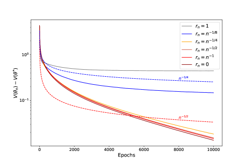
To illustrate Theorem 4.1 and the impact of bias, we consider in Figure 1 a simple least squares objective function $V(\theta)=\|A\theta\|^{2}/2$ in dimension $d=10$. We artificially add to every gradient a zero-mean Gaussian noise and a bias term $r_{n}=n^{-\alpha}$ at each iteration $n$. We use Adagrad with a learning rate $\gamma=1/2$, $\beta=0$ and $\lambda=0$. Then, the bound of Theorem 4.1 is of the form $\mathcal{O}(n^{-1/2}+n^{-2\alpha})$. First, note that the impact of a constant bias term ($r_{n}=1$) never vanishes. From $r_{n}=1$ to $r_{n}=n^{-1/4}$, the effect of the bias decreases until a threshold is reached where there is no significant improvement. The convergence rate in the case $r_{n}=n^{-1/4}$ is then the same as in the case without bias, illustrating the fact that in this case the dominating term comes from the learning rate.


Refer to caption

Figure 1: Value of $V(\theta_{n})-V(\theta^{*})$ with Adagrad for different values of $r_{n}=n^{-\alpha}$ and a learning rate $\gamma_{n}=n^{-1/2}$. The dashed curve corresponds to the expected convergence rate $\mathcal{O}(n^{-1/4})$ for $\alpha=1/8$ and $\mathcal{O}(n^{-1/2})$ for $\alpha\geq 1/4$.

Finally, note that non-adaptive SGD is a particular case of Theorem 4.1. Thus, our theorem gives new results also in the non-adaptive case with generic step sizes and biased gradients, while the only existing results in the literature assume constant step sizes (Ajalloeian and Stich,, 2020).

4.2 Non-convex smooth case

In the non-convex smooth case, the theoretical results are based on a randomized version of Stochastic Approximation as described by Nemirovski et al., (2009); Ghadimi and Lan, (2013); Karimi et al., (2019). In classical SA, the update (3) is performed a fixed number of times $n$, and the quantity of interest is the last parameter $\theta_{n}$. On the other hand, in Randomized Stochastic Approximation, we introduce a random variable $R$ which takes its values in $\{1,\dots,n\}$ and the quantity of interest is $\theta_{R}$. We stress that this procedure is a technical tool for the proofs, in practical applications we will always use classical SA.

The following theorem provides a bound in expectation on the gradient of the objective function $V$, which is the best results we can have given that no assumption is made about existence of a global minimum of $V$.

Theorem 4.2.

Assume that for all $k\geq 0$, we have $\gamma_{k+1}\leq\lambda_{k+1}/(6L\beta_{k+1}^{2})$. For any $n\geq 1$, let $R\in\{0,\ldots,n\}$ be a discrete random variable, independent of $\{\mathcal{F}_{n},n\in\mathbb{N}\}$, such that:

$$\mathbb{P}(R=k):=\frac{\gamma_{k+1}\lambda_{k+1}}{\sum_{j=0}^{n}\gamma_{j+1}\lambda_{j+1}}\;.$$

Then, under Assumptions 2424\ref{ass:A2}-\ref{ass:A4}, we have:

$$\mathbb{E}\left[\left\|\nabla V\left(\theta_{R}\right)\right\|^{2}\right]\leq 3\frac{V^{*}+\alpha_{1,n}/2+L\alpha_{2,n}}{\sum_{j=0}^{n}\gamma_{j+1}\lambda_{j+1}}\;,$$

where

$\displaystyle\alpha_{1,n}=\sum_{k=0}^{n}\gamma_{k+1}\beta_{k+1}^{2}r_{k}^{2}/\lambda_{k+1},\quad\alpha_{2,n}=\sum_{k=0}^{n}\gamma_{k+1}^{2}\beta_{k+1}^{2}\sigma_{k}^{2},$
$\displaystyle\text{and}\quad V^{*}=\mathbb{E}[V(\theta_{0})-V(\theta^{*})].$

Theorem 4.2 recovers the asymptotic rate of convergence obtained by Karimi et al., (2019) but with explicit bounds with respect to the hyper-parameters $\gamma,\beta,\lambda$ and the bias. We can observe that if $\gamma\leq\lambda+2\beta$, the condition on $(\gamma_{k})_{k\geq 1}$ can be met simply by tuning $C_{\gamma}$. In particular, if $A_{n}=\mathit{I}_{d}$, the requirement on the step sizes can be expressed as $\gamma_{k+1}\leq 1/(6L)$.

We give below the convergence rates obtained from Theorem 4.2 under the same assumptions on $\gamma_{n}$, $\beta_{n}$ and $\lambda_{n}$ as in the convex case.

Corollary 4.3.

Let $\gamma_{n}=C_{\gamma}n^{-\gamma},\beta_{n}=C_{\beta}n^{\beta},\lambda_{n}=C_{\lambda}n^{-\lambda}$ with $C_{\gamma}>0,C_{\beta}>0$, and $C_{\lambda}>0$. Assume that $\gamma,\beta,\lambda\geq 0$ and $\gamma+\lambda<1$. Then, under Assumptions 2424\ref{ass:A2}-\ref{ass:A4}, we have:

$$\mathbb{E}\left[\left\|\nabla V\left(\theta_{R}\right)\right\|^{2}\right]\!=\begin{cases}\mathcal{O}\left(n^{-\gamma+\lambda+2\beta}+b_{n}\right)\quad\text{if }\vartheta<1/2\;,\\ \mathcal{O}\left(n^{\gamma+\lambda-1}+b_{n}\right)\quad\quad\text{if }\vartheta>1/2\;,\\ \mathcal{O}\left(n^{\gamma+\lambda-1}\!\log n+b_{n}\right)\text{if }\vartheta=1/2\;,\end{cases}$$

with $\vartheta=\gamma-\beta$ and where the bias term $b_{n}$ can be constant or decreasing. In the latter case, writing $r_{n}=n^{-\alpha}$, we have:

$$b_{n}=\begin{cases}\mathcal{O}\left(n^{\beta-2\alpha}\right)&\text{if }2\alpha<1-\gamma+\lambda+2\beta\;,\\ \mathcal{O}\left(n^{\gamma+\lambda-1}\right)&\text{if }2\alpha>1-\gamma+\lambda+2\beta\;,\\ \mathcal{O}\left(n^{\gamma+\lambda-1}\log n\right)&\text{if }2\alpha=1-\gamma+\lambda+2\beta\;.\end{cases}$$

In practice, the value of $\alpha$ is known in advance while the other parameters can be tuned to achieve the optimal rate of convergence. In any scenario, we can never achieve a bound of $\mathcal{O}(1/\sqrt{n}+b_{n})$, and the best rate we can achieve is $\mathcal{O}(\log n/\sqrt{n}+b_{n})$ if and only if $\gamma=1/2,\beta=0$ and $\lambda=0$. In this case, all eigenvalues of $A_{n}$ must be bounded both from below and above. In the context of decreasing bias, if $\alpha\geq 1/4$, the bias term contributes to the speed of the algorithm. Otherwise, the other term is the leading term of the upper bound. However, in both cases, the best achievable bound is $\mathcal{O}(\log n/\sqrt{n})$ if $\alpha\geq 1/4$.

Bounded Gradient Case. Now, we provide the convergence analysis of Randomized Adaptive Stochastic Approximation with a bounded stochastic update. Consider the following additional assumption about the stochastic update.

Assumption 5.

The stochastic update is bounded, i.e., there exists $M\geq 0$ such that for all $n\in\mathbb{N}$,

$$\left\|H_{\theta_{n}}\left(X_{n+1}\right)\right\|\leq M.$$

It is important to note that under Assumption 3, this is equivalent to bounding the stochastic gradient of the objective function. Corollary 4.4 provides a bound on the gradient of the objective function $V$, which is similar to Theorem 4.2.

Corollary 4.4.

Let $\gamma_{n}=C_{\gamma}n^{-\gamma},\beta_{n}=C_{\beta}n^{\beta},\lambda_{n}=C_{\lambda}n^{-\lambda}$ with $C_{\gamma}>0,C_{\beta}>0$, and $C_{\lambda}>0$. Assume that $\gamma,\beta,\lambda\geq 0$ and $\gamma+\lambda<1$. For any $n\geq 1$, let $R\in\{0,\ldots,n\}$ be a uniformly distributed random variable. Then, under Assumptions 24,5245\ref{ass:A2}-\ref{ass:A4},\ref{ass:A5}, we have:

$$\mathbb{E}\left[\left\|\nabla V\left(\theta_{R}\right)\right\|^{2}\right]\leq\frac{2V^{*}+\alpha_{1,n}+LM^{2}\alpha_{2,n}^{\prime}}{\sqrt{n}}\;,$$

where $V^{*},\alpha_{1,n}$ are defined in Theorem 4.2 and $\alpha_{2,n}^{\prime}=\sum_{k=0}^{n}\gamma_{k+1}^{2}\beta_{k+1}^{2}.$

Importantly, in Corollary 4.4, there are no assumptions on the step sizes, and we obtain a better bound than in Theorem 4.2.

4.3 Application to Adagrad and RMSProp

In this section, we provide the convergence analysis of Adagrad and RMSProp with a biased gradient estimator.

Remark 4.5.

Under Assumption 5, for all eigenvalues $\lambda$ of $A_{n}$, the adaptive matrix in Adagrad or RMSProp, it holds that $(M^{2}+\delta)^{-1/2}\leq\lambda\leq\delta^{-1/2}$, i.e., Assumption 4 is satisfied with $\lambda=0$ and $\beta=0$.

Corollary 4.6.

Let $\gamma_{n}=c_{\gamma}n^{-1/2}$ and $A_{n}$ denote the adaptive matrix in Adagrad or RMSProp. For any $n\geq 1$, let $R\in\{0,\ldots,n\}$ be a uniformly distributed random variable. Then, under Assumptions 2,3,5235\ref{ass:A2},\ref{ass:A3},\ref{ass:A5}, we have:

$$\mathbb{E}\left[\left\|\nabla V\left(\theta_{R}\right)\right\|^{2}\right]=\mathcal{O}\left(\frac{\log n}{\sqrt{n}}+b_{n}\right).$$

The bias $b_{n}$ is explicitly given in Appendix A.

Since we do not have information about the global minimum of the objective function $V$, Corollary 4.6 establishes the rate of convergence of Adagrad and RMSProp with biased gradient to a critical point for non-convex smooth functions. In the case of an unbiased gradient, we obtain the same bound as in Zou et al., (2018), under the same assumptions:

$$\mathbb{E}\left[\left\|\nabla V\left(\theta_{R}\right)\right\|^{2}\right]=\mathcal{O}\left(\frac{\log n}{\sqrt{n}}\right).$$

If the bias is of the order $\mathcal{O}(n^{-1/4})$, the algorithm achieves the same convergence rate as in the case of an unbiased gradient.

5 Experiments

In this section, we illustrate our theoretical results in the context of deep VAE. The experiments were conducted using PyTorch (Paszke et al.,, 2017), and the source code can be found here***URL hidden during review process. In generative models, the objective is to maximize the marginal likelihood defined as:

$$\log p_{\theta}(x)=\log\mathbb{E}_{p_{\theta}(\cdot|x)}\left[\frac{p_{\theta}(x,Z)}{p_{\theta}(Z|x)}\right],$$

where $(x,z)\mapsto p_{\theta}(x,z)$ is the complete likelihood, $x$ are the observations and $Z$ is the latent variable. Under some simple technical assumptions, by Fisher’s identity, we have:

$$\nabla_{\theta}\log p_{\theta}(x)=\int\nabla_{\theta}\log p_{\theta}(x,z)p_{\theta}(z\mid x)\mathrm{d}z.$$ (7)

However, in most cases, the conditional density $z\mapsto p_{\theta}(z\mid x)$ is intractable and can only be sampled. Variational Autoencoders introduce an additional parameter $\phi$ and a family of variational distributions $z\mapsto q_{\phi}(z\mid x)$ to approximate the true posterior distribution. Parameters are estimated by maximizing the Evidence Lower Bound (ELBO):

$$\log p_{\theta}(x)\geq\mathbb{E}_{q_{\phi}(\cdot|x)}\left[\log\frac{p_{\theta}(x,Z)}{q_{\phi}(Z|x)}\right]=:\mathcal{L}_{\text{ELBO}}(\theta,\phi;x).$$

The Importance Weighted Autoencoder (IWAE) (Burda et al.,, 2015) is a variant of the VAE that incorporates importance weighting to obtain a tighter ELBO. The IWAE objective can be written as follows:

$$\mathcal{L}^{\text{IWAE}}_{k}(\theta,\phi;x)=\mathbb{E}_{q^{\otimes k}_{\phi}(\cdot|x)}\left[\log\frac{1}{k}\sum_{\ell=1}^{k}\frac{p_{\theta}(x,Z^{(\ell)})}{q_{\phi}(Z^{(\ell)}|x)}\right],$$

where $k$ corresponds to the number of samples drawn from the variational posterior distribution. The estimator of the gradient of ELBO in IWAE corresponds to the biased Self-Normalized Importance Sampling (SNIS) estimator of the gradient of the marginal log likelihood $\log p_{\theta}(x)$. As a consequence of the results of Agapiou et al., (2017), both the bias and Mean Squared Error (MSE) are of order $\mathcal{O}(1/k)$. Since the bias has an impact on the convergence rates, we propose to use the Biased Reduced Self-Normalized Importance Sampling (BR-SNIS) algorithm, proposed by Cardoso et al., (2022), to the IWAE estimator, resulting in the Biased Reduced Importance Weighted Autoencoder (BR-IWAE). The BR-IWAE algorithm (Cardoso et al.,, 2022) proceeds in two steps, which are repeated during optimization:

  • Update the parameter $\phi$ as in the IWAE algorithm, that is, for all $n\geq 1$:

    $$\phi_{n+1}=\phi_{n}-\gamma_{n+1}A_{n}\nabla_{\phi}\mathcal{L}^{\text{IWAE}}_{k}(\theta_{n},\phi_{n};X_{n+1}).$$
  • Update the parameter $\theta$ by estimating (7) using BR-SNIS as detailed in Appendix B.

Dataset. We conduct our experiments on the CIFAR-10 dataset (Krizhevsky et al.,, 2009), which is a widely used dataset for image classification tasks. CIFAR-10 consists of 32x32 pixel images categorized into 10 different classes. The dataset is divided into 60,000 images in the training set and 10,000 images in the test set. Additional experiments are provided in Appendix B.

Model. We use a Convolutional Neural Network (CNN) architecture with the Rectified Linear Unit (ReLU) activation function for both the encoder and the decoder. The latent space dimension is set to 100. Further details of the model are provided in Appendix B. We estimate the log-likelihood using the VAE, IWAE, and BR-IWAE models, all of which are trained for 100 epochs. Training is conducted using Adagrad and RMSProp with a decaying learning rate.


Refer to caption

Figure 2: Negative Log-Likelihood on the test set for Different Generative Models with Adagrad and RMSProp on the CIFAR-10 Dataset. Bold lines represent the mean over 5 independent runs.

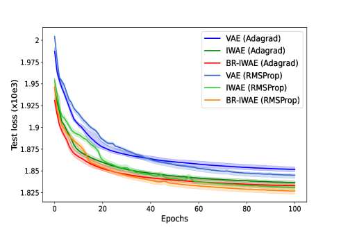
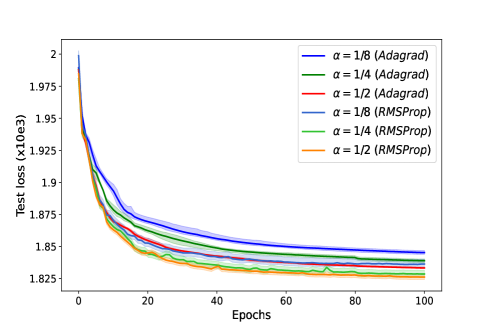
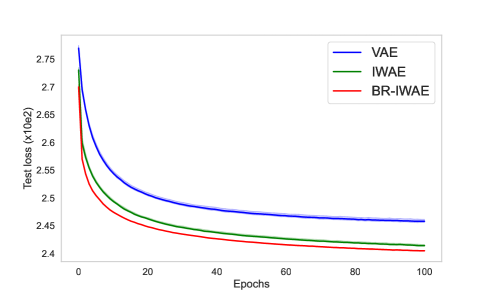
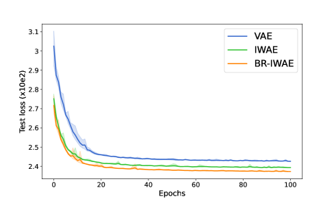
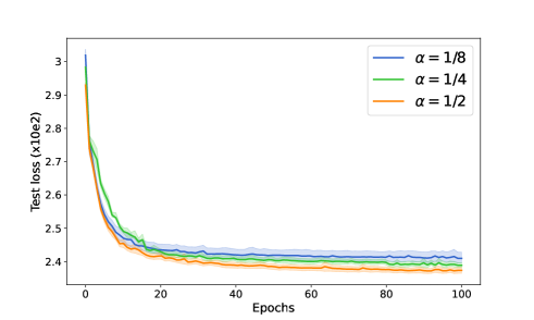
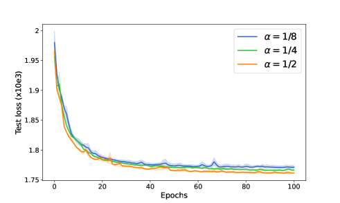
In this section, we exclusively use Adagrad and RMSProp algorithms to illustrate the results of Section 4.3 and we do not conduct a comparison with SGD. For the first experiment, we set a constant bias, i.e., we use $k=5$ samples in both IWAE and BR-IWAE, while restricting the maximum iteration of the MCMC algorithm to 5 for BR-IWAE. The test losses are presented in Figure 2. We show the negative log-likelihood on the test dataset for VAE, IWAE, and BR-IWAE with Adagrad and RMSProp. As expected, we observe that IWAE outperforms VAE, while BR-IWAE outperforms IWAE by reducing bias in both cases.

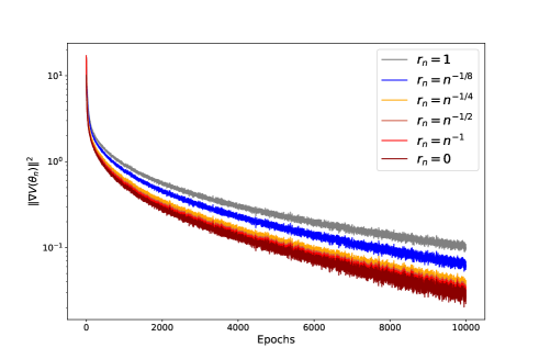
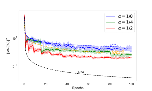
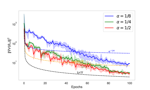
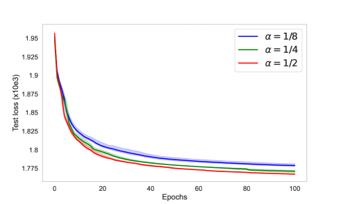
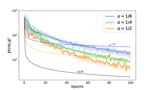
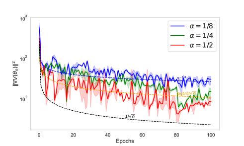
To illustrate our results, we choose to incorporate a time-dependent bias that decreases by choosing a bias of order $\mathcal{O}(n^{-\alpha})$ at iteration $n$. The bias of the estimator of the gradient in IWAE is of the order $\mathcal{O}(1/k)$, where $k$ is the number of importance weights. Therefore, choosing the bias of order $\mathcal{O}(n^{-\alpha})$ is equivalent to using $n^{\alpha}$ samples at iteration $n$, to estimate the gradient. This procedure is detailed in Appendix B. We vary $\alpha$ only for IWAE for computational efficiency and plot the following quantities.

  • In Figures 3 and 4, the gradient squared norm $\|\nabla V(\theta_{n})\|^{2}$ to illustrate the convergence rate.

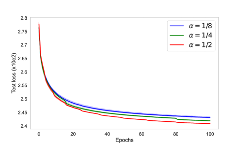
  • In Figure 5, the Negative Log-Likelihood along iterations.

Figures 3 and 4 illustrate our results, while the other figures are meant to confirm the behavior of test loss with different values of $\alpha$. All figures are plotted on a logarithmic scale for better visualization. It is important to note that all figures are in respect to epochs, whereas here, $n$ represents the iteration (number of updates of the gradient).


Refer to caption

Figure 3: Value of $\|\nabla V(\theta_{n})\|^{2}$ in IWAE with Adagrad for different values of $\alpha$. Bold lines represent the mean over 5 independent runs.

Refer to caption

Figure 4: Value of $\|\nabla V(\theta_{n})\|^{2}$ in IWAE with RMSProp and Adam for different values of $\alpha$. Bold lines represent the mean over 5 independent runs.

Refer to caption

Figure 5: Negative Log-Likelihood on the test set on the CIFAR-10 Dataset for IWAE with Adagrad and RMSProp for Different Values of $\alpha$. Bold lines represent the mean over 5 independent runs.

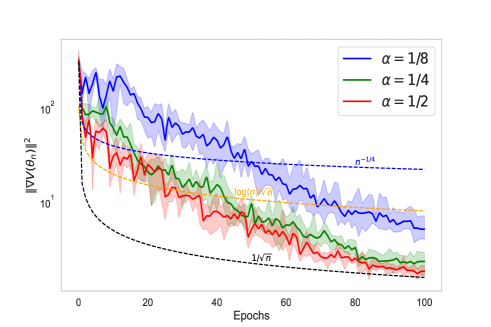
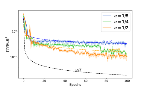
Note that the dashed curve corresponds to the expected convergence rate $\mathcal{O}(n^{-1/4})$ for $\alpha=1/8$ and $\mathcal{O}(\log n/\sqrt{n})$ for $\alpha=1/4$ and for $\alpha=1/2$. We can clearly observe that for each of the cases, fast convergence is achieved when $n$ is sufficiently large. There are several possible explanations for this rapid convergence with a decreasing time-dependent bias. First, we may be able to improve the upper bound by obtaining for instance a better bound for the bias.

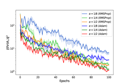
Our experiments show similar results for Adagrad and RMSProp in terms of convergence rates, although RMSProp performs slightly better. However, Adam’s behavior is somewhat more intricate due to the incorporation of momentum. Nevertheless, we consistently observe the impact of bias, although it tends to be relatively small, as the bias correction terms may help mitigate bias in the moving averages.
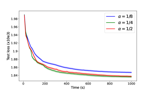
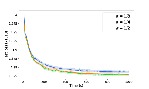
It is clear that with a larger $\alpha$, convergence in both squared gradient norm and negative log-likelihood is faster. However, beyond a certain threshold for $\alpha$, we observe that the rate of convergence does not change significantly. Since choosing a larger $\alpha$ induces an additional computational cost, it is crucial to select an appropriate value of $\alpha$, that achieves fast convergence without being too computationally costly. One approach to choose such a value for $\alpha$ is to plot the test loss with respect to time, which is shown in Figure 6 for Adagrad. Although $\alpha=1/2$ seems to have faster convergence in terms of iterations in Figure 5, the best rate in terms of time in Figure 6 is $\alpha=1/4$. We obtain similar results for RMSProp, see Appendix B.


Refer to caption

Figure 6: Negative Log-Likelihood on the test set of the CIFAR-10 Dataset for IWAE with Adagrad for Different Values of $\alpha$ over time (in seconds). Bold lines represent the mean over 5 independent runs.

6 Discussion

This paper provides a comprehensive non-asymptotic analysis of Biased Adaptive Stochastic Approximation for both convex and non-convex smooth functions. We derive a convergence rate of $\mathcal{O}(1/\sqrt{n}+b_{n})$ for convex functions and $\mathcal{O}(\log n/\sqrt{n}+b_{n})$ for non-convex smooth functions, where $b_{n}$ corresponds to the time-dependent decreasing bias. We also establish that Adagrad and RMSProp with biased gradients converges to critical points for non-convex smooth functions. Our results provide insights on hyper-parameters tuning to achieve fast convergence and reduce unnecessary computational time.

We intend to investigate whether the eigenvalues control conditions can be satisfied in practical settings, such as in the case of Stochastic Newton or Gauss Newton methods. We conducted additional comparisons with Adam to propose practical insights. However, a possible extension of our work is to extend our theoretical results to Adam.

References

  • Agapiou et al., (2017) Agapiou, S., Papaspiliopoulos, O., Sanz-Alonso, D., and Stuart, A. M. (2017). Importance sampling: Intrinsic dimension and computational cost. Statistical Science, pages 405–431.
  • Ajalloeian and Stich, (2020) Ajalloeian, A. and Stich, S. U. (2020). On the Convergence of SGD with Biased Gradients. arXiv preprint arXiv:2008.00051.
  • Auer et al., (2002) Auer, P., Cesa-Bianchi, N., and Gentile, C. (2002). Adaptive and self-confident on-line learning algorithms. Journal of Computer and System Sciences, 64(1):48–75.
  • Baxter and Bartlett, (2001) Baxter, J. and Bartlett, P. L. (2001). Infinite-horizon policy-gradient estimation. Journal of Artificial Intelligence Research, 15:319–350.
  • Bhandari et al., (2018) Bhandari, J., Russo, D., and Singal, R. (2018). A finite time analysis of temporal difference learning with linear function approximation. In Conference On Learning Theory, pages 1691–1692. PMLR.
  • Bottou, (1991) Bottou, L. (1991). Une approche théorique de l’apprentissage connexioniste; applications à la reconnaissance de la parole. PhD thesis, Paris 11.
  • Bottou et al., (2018) Bottou, L., Curtis, F. E., and Nocedal, J. (2018). Optimization methods for large-scale machine learning. SIAM Review, 60(2):223–311.
  • Boyer and Godichon-Baggioni, (2023) Boyer, C. and Godichon-Baggioni, A. (2023). On the asymptotic rate of convergence of stochastic newton algorithms and their weighted averaged versions. Computational Optimization and Applications, 84(3):921–972.
  • Burda et al., (2015) Burda, Y., Grosse, R., and Salakhutdinov, R. (2015). Importance weighted autoencoders. arXiv preprint arXiv:1509.00519.
  • Cardoso et al., (2023) Cardoso, G., Idrissi, Y. J. E., Le Corff, S., Moulines, É., and Olsson, J. (2023). State and parameter learning with PaRIS particle Gibbs. arXiv preprint arXiv:2301.00900.
  • Cardoso et al., (2022) Cardoso, G., Samsonov, S., Thin, A., Moulines, E., and Olsson, J. (2022). BR-SNIS: bias reduced self-normalized importance sampling. Advances in Neural Information Processing Systems, 35:716–729.
  • Chen et al., (2017) Chen, P.-Y., Zhang, H., Sharma, Y., Yi, J., and Hsieh, C.-J. (2017). Zoo: Zeroth order optimization based black-box attacks to deep neural networks without training substitute models. In Proceedings of the 10th ACM Workshop on Artificial Intelligence and Security, pages 15–26.
  • Dalal et al., (2018) Dalal, G., Szörényi, B., Thoppe, G., and Mannor, S. (2018). Finite sample analyses for td (0) with function approximation. In Proceedings of the AAAI Conference on Artificial Intelligence, volume 32.
  • Défossez et al., (2020) Défossez, A., Bottou, L., Bach, F., and Usunier, N. (2020). A simple convergence proof of Adam and Adagrad. arXiv preprint arXiv:2003.02395.
  • Del Moral et al., (2010) Del Moral, P., Doucet, A., and Singh, S. S. (2010). A backward particle interpretation of Feynman-Kac formulae. ESAIM: Mathematical Modelling and Numerical Analysis, 44(5):947–975.
  • Doan et al., (2020) Doan, T. T., Nguyen, L. M., Pham, N. H., and Romberg, J. (2020). Finite-time analysis of stochastic gradient descent under markov randomness. arXiv preprint arXiv:2003.10973.
  • Dozat, (2016) Dozat, T. (2016). Incorporating Nesterov momentum into Adam.
  • Duchi et al., (2011) Duchi, J., Hazan, E., and Singer, Y. (2011). Adaptive subgradient methods for online learning and stochastic optimization. Journal of Machine Learning Research, 12(7).
  • Ghadimi and Lan, (2013) Ghadimi, S. and Lan, G. (2013). Stochastic first-and zeroth-order methods for nonconvex stochastic programming. SIAM Journal on Optimization, 23(4):2341–2368.
  • Gloaguen et al., (2022) Gloaguen, P., Le Corff, S., and Olsson, J. (2022). A pseudo-marginal sequential Monte Carlo online smoothing algorithm. Bernoulli, 28(4):2606–2633.
  • Godichon-Baggioni and Tarrago, (2023) Godichon-Baggioni, A. and Tarrago, P. (2023). Non asymptotic analysis of adaptive stochastic gradient algorithms and applications. arXiv preprint arXiv:2303.01370.
  • Jaakkola et al., (1993) Jaakkola, T., Jordan, M., and Singh, S. (1993). Convergence of stochastic iterative dynamic programming algorithms. Advances in Neural Information Processing Systems, 6.
  • Karimi et al., (2019) Karimi, B., Miasojedow, B., Moulines, E., and Wai, H.-T. (2019). Non-asymptotic analysis of biased stochastic approximation scheme. In Conference on Learning Theory, pages 1944–1974. PMLR.
  • Kingma and Ba, (2014) Kingma, D. P. and Ba, J. (2014). Adam: A method for stochastic optimization. arXiv preprint arXiv:1412.6980.
  • Kingma and Welling, (2013) Kingma, D. P. and Welling, M. (2013). Auto-encoding variational bayes. arXiv preprint arXiv:1312.6114.
  • Kresoja et al., (2017) Kresoja, M., Lužanin, Z., and Stojkovska, I. (2017). Adaptive stochastic approximation algorithm. Numerical Algorithms, 76(4):917–937.
  • Krizhevsky et al., (2009) Krizhevsky, A., Hinton, G., et al. (2009). Learning multiple layers of features from tiny images.
  • Lakshminarayanan and Szepesvari, (2018) Lakshminarayanan, C. and Szepesvari, C. (2018). Linear stochastic approximation: How far does constant step-size and iterate averaging go? In International Conference on Artificial Intelligence and Statistics, pages 1347–1355. PMLR.
  • Li and Wai, (2022) Li, Q. and Wai, H.-T. (2022). State dependent performative prediction with stochastic approximation. In International Conference on Artificial Intelligence and Statistics, pages 3164–3186. PMLR.
  • Moosavi-Dezfooli et al., (2017) Moosavi-Dezfooli, S.-M., Fawzi, A., Fawzi, O., and Frossard, P. (2017). Universal adversarial perturbations. In Proceedings of the IEEE Conference on Computer Vision and Pattern Recognition, pages 1765–1773.
  • Moulines and Bach, (2011) Moulines, E. and Bach, F. (2011). Non-asymptotic analysis of stochastic approximation algorithms for machine learning. Advances in Neural Information Processing Systems, 24.
  • Nemirovski et al., (2009) Nemirovski, A., Juditsky, A., Lan, G., and Shapiro, A. (2009). Robust stochastic approximation approach to stochastic programming. SIAM Journal on Optimization, 19(4):1574–1609.
  • Nemirovskij and Yudin, (1983) Nemirovskij, A. S. and Yudin, D. B. (1983). Problem complexity and method efficiency in optimization.
  • Nesterov and Spokoiny, (2017) Nesterov, Y. and Spokoiny, V. (2017). Random gradient-free minimization of convex functions. Foundations of Computational Mathematics, 17:527–566.
  • Olsson and Westerborn, (2017) Olsson, J. and Westerborn, J. (2017). Efficient particle-based online smoothing in general hidden Markov models: the paris algorithm.
  • Paszke et al., (2017) Paszke, A., Gross, S., Chintala, S., Chanan, G., Yang, E., DeVito, Z., Lin, Z., Desmaison, A., Antiga, L., and Lerer, A. (2017). Automatic differentiation in PyTorch.
  • Polyak and Juditsky, (1992) Polyak, B. T. and Juditsky, A. B. (1992). Acceleration of stochastic approximation by averaging. SIAM Journal on Control and Optimization, 30(4):838–855.
  • Robbins and Monro, (1951) Robbins, H. and Monro, S. (1951). A stochastic approximation method. The Annals of Mathematical Statistics, pages 400–407.
  • Sun et al., (2018) Sun, T., Sun, Y., and Yin, W. (2018). On Markov chain gradient descent. Advances in Neural Information Processing Systems, 31.
  • Tadić and Doucet, (2011) Tadić, V. B. and Doucet, A. (2011). Asymptotic bias of stochastic gradient search. In 2011 50th IEEE Conference on Decision and Control and European Control Conference, pages 722–727. IEEE.
  • Tieleman et al., (2012) Tieleman, T., Hinton, G., et al. (2012). Lecture 6.5-rmsprop: Divide the gradient by a running average of its recent magnitude. COURSERA: Neural Networks for Machine Learning, 4(2):26–31.
  • Tjelmeland, (2004) Tjelmeland, H. (2004). Using all metropolis–hastings proposals to estimate mean values. Technical report.
  • Ward et al., (2020) Ward, R., Wu, X., and Bottou, L. (2020). Adagrad stepsizes: Sharp convergence over nonconvex landscapes. The Journal of Machine Learning Research, 21(1):9047–9076.
  • Xiao et al., (2017) Xiao, H., Rasul, K., and Vollgraf, R. (2017). Fashion-mnist: a novel image dataset for benchmarking machine learning algorithms. arXiv preprint arXiv:1708.07747.
  • Zeiler, (2012) Zeiler, M. D. (2012). Adadelta: an adaptive learning rate method. arXiv preprint arXiv:1212.5701.
  • Zou et al., (2018) Zou, F., Shen, L., Jie, Z., Sun, J., and Liu, W. (2018). Weighted adagrad with unified momentum. arXiv preprint arXiv:1808.03408.

Appendix A Proofs

A.1 Proof of Theorem 4.1

We first establish a technical lemma which is essential for the proof.

Lemma A.1.

Let $\left(\delta_{n}\right)_{n\geq 0},\left(\gamma_{n}\right)_{n\geq 1},\left(\eta_{n}\right)_{n\geq 1}$, and $\left(v_{n}\right)_{n\geq 1}$ be some positive sequences satisfying the following assumptions.

  • The sequence $\delta_{n}$ follows the recursive relation:

    $$\delta_{n}\leq\left(1-2\omega\gamma_{n}+\eta_{n}\gamma_{n}\right)\delta_{n-1}+v_{n}\gamma_{n},$$

    with $\delta_{0}\geq 0$ and $\omega>0$.

  • Let $n_{0}=\inf\left\{n\geq 1:\eta_{n}\leq\omega\right\}$, then for all $n\geq n_{0}+1$, we assume that $\omega\gamma_{n}\leq 1$.

Then, for all $n\in\mathbb{N}$,

$$\delta_{n}\leq\exp\left(-\omega\sum_{k=n/2}^{n}\gamma_{k}\right)\exp\left(2\sum_{k=1}^{n}\eta_{k}\gamma_{k}\right)\left(\delta_{0}+2\max_{1\leq k\leq n}\frac{v_{k}}{\eta_{k}}\right)+\frac{1}{\omega}\max_{n/2\leq k\leq n}v_{k}.$$

The proof is given in Godichon-Baggioni and Tarrago, (2023). We will present the detailed version of Theorem 4.1.

Theorem A.2.

Let $\theta_{n}\in\mathbb{R}^{d}$ be the $n$-th iterate of the recursion (3). Under Assumptions 1414\ref{ass:A1}-\ref{ass:A4}, we have:

$\displaystyle\mathbb{E}\left[V\left(\theta_{n}\right)-V(\theta^{*})\right]$ $\displaystyle\leq\left(\mathbb{E}\left[V\left(\theta_{0}\right)-V(\theta^{*})\right]+\frac{1}{L^{2}}\max_{1\leq k\leq n}\frac{\lambda_{k+1}v_{k}}{\beta_{k+1}^{2}\gamma_{k+1}}\right)\exp{\left(-\frac{\mu}{2}\sum_{k=n/2}^{n}\lambda_{k+1}\gamma_{k+1}\right)}$
$\displaystyle\quad\exp{\left(4L^{2}\sum_{k=1}^{n}C_{k}\beta_{k+1}^{2}\gamma_{k+1}^{2}\right)}+\frac{2}{\mu}\max_{n/2\leq k\leq n}v_{k},$

where

$$C_{k}=\max\left\{1,\frac{\mu^{2}\lambda_{k+1}^{2}}{8L^{2}\beta_{k+1}^{2}}\right\}\quad\mathrm{and}\quad v_{k}=\frac{1}{2}\frac{L\beta_{k+1}^{2}r_{k}^{2}}{\mu\lambda_{k+1}^{2}}+L\sigma_{k}^{2}\frac{\beta_{k+1}^{2}}{\lambda_{k+1}}\gamma_{k+1}.$$
Proof.

As $V$ is $L$ smooth (Assumption 2) and using the recursion (3)italic-(3italic-)\eqref{ASA} of Adaptive SA, we obtain:

$\displaystyle V\left(\theta_{n+1}\right)$ $\displaystyle\leq V\left(\theta_{n}\right)+\left\langle\nabla V\left(\theta_{n}\right)\mid\theta_{n+1}-\theta_{n}\right\rangle+\frac{L}{2}\left\|\theta_{n+1}-\theta_{n}\right\|^{2}$
$\displaystyle\leq V\left(\theta_{n}\right)-\gamma_{n+1}\left\langle\nabla V\left(\theta_{n}\right)\mid A_{n}H_{\theta_{n}}\left(X_{n+1}\right)\right\rangle+\frac{L\gamma_{n+1}^{2}}{2}\left\|A_{n}\right\|^{2}\left\|H_{\theta_{n}}\left(X_{n+1}\right)\right\|^{2}$
$\displaystyle\leq V\left(\theta_{n}\right)-\gamma_{n+1}\left\langle\nabla V\left(\theta_{n}\right)\mid A_{n}H_{\theta_{n}}\left(X_{n+1}\right)\right\rangle+\frac{L\gamma_{n+1}^{2}}{2}\beta_{n+1}^{2}\left\|H_{\theta_{n}}\left(X_{n+1}\right)-\nabla V\left(\theta_{n}\right)+\nabla V\left(\theta_{n}\right)\right\|^{2}.$

Using that for all $x$, $y\geq 0$, $\left\|x+y\right\|^{2}\leq 2\left(\left\|x\right\|^{2}+\left\|y\right\|^{2}\right)$, and writing $V_{n}=V\left(\theta_{n}\right)-V(\theta^{*})$, we get

$$V_{n+1}\leq V_{n}-\gamma_{n+1}\left\langle\nabla V\left(\theta_{n}\right)\mid A_{n}H_{\theta_{n}}\left(X_{n+1}\right)\right\rangle+L\gamma_{n+1}^{2}\beta_{n+1}^{2}\left(\left\|H_{\theta_{n}}\left(X_{n+1}\right)-\nabla V\left(\theta_{n}\right)\right\|^{2}+\left\|\nabla V\left(\theta_{n}\right)\right\|^{2}\right).$$

Then, using Assumption 3, and since $\left\|\nabla V\left(\theta_{n}\right)\right\|^{2}\leq 2LV_{n}$ (Assumption 1 and 2),

$\displaystyle\mathbb{E}\left[V_{n+1}\mid\mathcal{F}_{n}\right]$ $\displaystyle\leq\left(1+2L^{2}\beta_{n+1}^{2}\gamma_{n+1}^{2}\right)V_{n}-\gamma_{n+1}\left\langle\nabla V\left(\theta_{n}\right)\mid A_{n}\left(\mathbb{E}\left[H_{\theta_{n}}\left(X_{n+1}\right)\mid\mathcal{F}_{n}\right]-\nabla V\left(\theta_{n}\right)\right)\right\rangle$
$\displaystyle\quad-\gamma_{n+1}\left\langle\nabla V\left(\theta_{n}\right)\mid A_{n}\nabla V\left(\theta_{n}\right)\right\rangle+L\sigma_{n}^{2}\gamma_{n+1}^{2}\beta_{n+1}^{2}$
$\displaystyle\leq\left(1+2L^{2}\beta_{n+1}^{2}\gamma_{n+1}^{2}\right)V_{n}+\gamma_{n+1}\beta_{n+1}r_{n}\left\|\nabla V\left(\theta_{n}\right)\right\|-\gamma_{n+1}\left\langle\nabla V\left(\theta_{n}\right)\mid A_{n}\nabla V\left(\theta_{n}\right)\right\rangle$
$\displaystyle\quad+L\sigma_{n}^{2}\gamma_{n+1}^{2}\beta_{n+1}^{2}$
$\displaystyle\leq\left(1+2L^{2}\beta_{n+1}^{2}\gamma_{n+1}^{2}\right)V_{n}+\frac{1}{2a_{n}}\gamma_{n+1}\beta_{n+1}r_{n}^{2}+a_{n}L\gamma_{n+1}\beta_{n+1}V_{n}$
$\displaystyle\quad-\gamma_{n+1}\left\langle\nabla V\left(\theta_{n}\right)\mid A_{n}\nabla V\left(\theta_{n}\right)\right\rangle+L\sigma_{n}^{2}\gamma_{n+1}^{2}\beta_{n+1}^{2},$

where the second last inequality is due to the Cauchy-Schwarz inequality. In the last inequality, we used $\left\|\nabla V\left(\theta_{n}\right)\right\|^{2}\leq 2LV_{n}$ and the inequality $xy\leq x^{2}/(2a_{n})+a_{n}y^{2}/2$ where $a_{n}$ is defined below. Furthermore, since $V$ satisfies the Polyak-Łojasiewicz condition (Assumption 1),

$$\left\langle\nabla V\left(\theta_{n}\right)\mid A_{n}\nabla V\left(\theta_{n}\right)\right\rangle\geq\lambda_{\min}\left(A_{n}\right)\left\|\nabla V\left(\theta_{n}\right)\right\|^{2}\geq 2\lambda_{n+1}\mu V_{n}.$$

Finally, choosing $a_{n}=(\mu\lambda_{n+1})/(L\beta_{n+1})$ we obtain:

$\displaystyle\mathbb{E}\left[V_{n+1}\right]\leq\left(1-\mu\lambda_{n+1}\gamma_{n+1}+2L^{2}\beta_{n+1}^{2}\gamma_{n+1}^{2}\right)\mathbb{E}\left[V_{n}\right]$ $\displaystyle+\frac{1}{2}\frac{L\beta_{n+1}^{2}r_{n}^{2}}{\mu\lambda_{n+1}}\gamma_{n+1}+L\sigma_{n}^{2}\gamma_{n+1}^{2}\beta_{n+1}^{2}.$

By choosing $\bar{\gamma}_{n+1}=\lambda_{n+1}\gamma_{n+1}$, we get:

$\displaystyle\mathbb{E}\left[V_{n+1}\right]\leq\left(1-\mu\bar{\gamma}_{n+1}+2L^{2}\frac{\beta_{n+1}^{2}}{\lambda_{n+1}^{2}}\bar{\gamma}_{n+1}^{2}\right)\mathbb{E}\left[V_{n}\right]$ $\displaystyle+\frac{1}{2}\frac{L\beta_{n+1}^{2}r_{n}^{2}}{\mu\lambda_{n+1}^{2}}\bar{\gamma}_{n+1}+L\sigma_{n}^{2}\frac{\beta_{n+1}^{2}}{\lambda_{n+1}^{2}}\bar{\gamma}_{n+1}^{2}.$

In order to satisfy the assumptions of Lemma A.1, consider $C_{n}=\max\left\{1,(\mu^{2}\lambda_{n+1}^{2})/(8L^{2}\beta_{n+1}^{2})\right\}$, and since $C_{n}\geq 1$, we have:

$\displaystyle\mathbb{E}\left[V_{n+1}\right]\leq\left(1-\mu\bar{\gamma}_{n+1}+2L^{2}\frac{C_{n}\beta_{n+1}^{2}}{\lambda_{n+1}^{2}}\bar{\gamma}_{n+1}^{2}\right)\mathbb{E}\left[V_{n}\right]$ $\displaystyle+\frac{1}{2}\frac{L\beta_{n+1}^{2}r_{n}^{2}}{\mu\lambda_{n+1}^{2}}\bar{\gamma}_{n+1}+L\sigma_{n}^{2}\frac{\beta_{n+1}^{2}}{\lambda_{n+1}^{2}}\bar{\gamma}_{n+1}^{2}.$

Now, using lemma A.1 by choosing:

$$\delta_{n}=\mathbb{E}\left[V_{n}\right],\quad\eta_{n}=2L^{2}\frac{C_{n}\beta_{n+1}^{2}}{\lambda_{n+1}^{2}}\bar{\gamma}_{n+1},\quad\omega=\frac{\mu}{2},\quad v_{n}=\frac{1}{2}\frac{L\beta_{n+1}^{2}r_{n}^{2}}{\mu\lambda_{n+1}^{2}}+L\sigma_{n}^{2}\frac{\beta_{n+1}^{2}}{\lambda_{n+1}^{2}}\bar{\gamma}_{n+1},$$

we have:

$$\mathbb{E}\left[V\left(\theta_{n}\right)-V(\theta^{*})\right]\leq\left(\mathbb{E}\left[V\left(\theta_{0}\right)-V(\theta^{*})\right]+\frac{1}{L^{2}}\max_{1\leq k\leq n}\frac{v_{k}\lambda_{k+1}^{2}}{\beta_{k+1}^{2}\bar{\gamma}_{k+1}}\right)e^{-\frac{\mu}{2}\sum_{k=n/2}^{n}\bar{\gamma}_{k+1}}e^{4L^{2}\sum_{k=1}^{n}\frac{C_{k}\beta_{k+1}^{2}}{\lambda_{k+1}^{2}}\bar{\gamma}_{k+1}^{2}}\\ +\frac{2}{\mu}\max_{n/2\leq k\leq n}\left\{v_{k}\right\},$$

which concludes the proof by replacing $\bar{\gamma}_{n+1}=\lambda_{n+1}\gamma_{n+1}$. ∎

A.2 Proof of Theorem 4.2

By Assumption 2, $V$ is $L$-smooth and using the recursion (3)italic-(3italic-)\eqref{ASA} of Adaptive SA together with a Taylor expansion, we obtain:

$\displaystyle V\left(\theta_{k+1}\right)\leq\,$ $\displaystyle V\left(\theta_{k}\right)+\left\langle\nabla V\left(\theta_{k}\right)\mid\theta_{k+1}-\theta_{k}\right\rangle+\frac{L}{2}\left\|\theta_{k+1}-\theta_{k}\right\|^{2},$

which yields

$\displaystyle V\left(\theta_{k+1}\right)$ $\displaystyle\leq V\left(\theta_{k}\right)-\gamma_{k+1}\left\langle\nabla V\left(\theta_{k}\right)\mid A_{k}\nabla V\left(\theta_{k}\right)\right\rangle-\gamma_{k+1}\left\langle\nabla V\left(\theta_{k}\right)\mid A_{k}\left(H_{\theta_{k}}\left(X_{k+1}\right)-\nabla V\left(\theta_{k}\right)\right)\right\rangle$
$\displaystyle\,\quad+\delta_{k+1}\big{(}\left\|H_{\theta_{k}}\left(X_{k+1}\right)-\nabla V\left(\theta_{k}\right)\right\|^{2}+\left\|\nabla V\left(\theta_{k}\right)\right\|^{2}\big{)},$

with $\delta_{k+1}=L\gamma_{k+1}^{2}\beta_{k+1}^{2}$. By the Cauchy-Schwarz inequality, and using Assumptions (3) and (4),

$\displaystyle\mathbb{E}[V(\theta_{k+1})|\mathcal{F}_{k}]$ $\displaystyle\leq V(\theta_{k})+\gamma_{k+1}\beta_{k+1}r_{k}\|\nabla V(\theta_{k})\|-\gamma_{k+1}\lambda_{\min}(A_{k})\|\nabla V(\theta_{k})\|^{2}+\delta_{k+1}(\sigma_{k}^{2}+\|\nabla V(\theta_{k})\|^{2}).$

Therefore,

$\displaystyle\gamma_{k+1}\left(\lambda_{k+1}-\frac{\lambda_{k+1}}{2}-L\gamma_{k+1}\beta_{k+1}^{2}\right)\left\|\nabla V\left(\theta_{k}\right)\right\|^{2}\leq V\left(\theta_{k}\right)-\mathbb{E}\left[V\left(\theta_{k+1}\right)|\mathcal{F}_{k}\right]+\frac{\gamma_{k+1}\beta_{k+1}^{2}r_{k}^{2}}{2\lambda_{k+1}}+\delta_{k+1}\sigma_{k}^{2}.$

and

$\displaystyle\sum_{k=0}^{n}\gamma_{k+1}\lambda_{k+1}\left(\frac{1}{2}-\frac{L\gamma_{k+1}\beta_{k+1}^{2}}{\lambda_{k+1}}\right)\mathbb{E}\left[\left\|\nabla V\left(\theta_{k}\right)\right\|^{2}\right]$ $\displaystyle\leq\mathbb{E}\left[V\left(\theta_{0}\right)-V\left(\theta_{n+1}\right)\right]+\frac{1}{2}\sum_{k=0}^{n}\frac{\gamma_{k+1}\beta_{k+1}^{2}r_{k}^{2}}{\lambda_{k+1}}+\sum_{k=0}^{n}\delta_{k+1}\sigma_{k}^{2}.$

Then, given that $\gamma_{k+1}\leq\lambda_{k+1}/(6L\beta_{k+1}^{2})$, we have

$\displaystyle\frac{1}{3}\mathbb{E}\left[\sum_{k=0}^{n}\gamma_{k+1}\lambda_{k+1}\left\|\nabla V\left(\theta_{k}\right)\right\|^{2}\right]$ $\displaystyle\leq\mathbb{E}\left[V\left(\theta_{0}\right)-V\left(\theta_{n+1}\right)\right]+\frac{1}{2}\sum_{k=0}^{n}\frac{\gamma_{k+1}\beta_{k+1}^{2}r_{k}^{2}}{\lambda_{k+1}}+\sum_{k=0}^{n}\delta_{k+1}\sigma_{k}^{2}\;.$

Consequently, by definition of the discrete random variable $R$,

$\displaystyle\mathbb{E}\left[\left\|\nabla V\left(\theta_{R}\right)\right\|^{2}\right]$ $\displaystyle=\sum_{k=0}^{n}\frac{\gamma_{k+1}\lambda_{k+1}\mathbb{E}\left[\left\|\nabla V\left(\theta_{k}\right)\right\|^{2}\right]}{\sum_{j=0}^{n}\gamma_{j+1}\lambda_{j+1}}$
$\displaystyle\,\leq 3\frac{V_{0,n}+\frac{1}{2}\sum_{k=0}^{n}\gamma_{k+1}\beta_{k+1}^{2}r_{k}^{2}/\lambda_{k+1}+\sum_{k=0}^{n}\delta_{k+1}\sigma_{k}^{2}}{\sum_{j=0}^{n}\gamma_{j+1}\lambda_{j+1}},$

where $V_{0,n}=\mathbb{E}[V(\theta_{0})-V(\theta_{n+1})]$, which concludes the proof by noting that $V(\theta_{n+1})\geq V(\theta^{*})$.

A.3 Proof of Corollary 4.3

The proof is a direct consequence of the fact that for a sufficiently large $n$:

$$\sum_{k=1}^{n}\frac{1}{k^{s}}=\begin{cases}\mathcal{O}\left(n^{-s+1}\right)&\text{if }0\leq s<1\;,\\ \mathcal{O}\left(1\right)&\text{if }s>1\;,\\ \mathcal{O}\left(\log n\right)&\text{if }s=1\;.\end{cases}$$

A.4 Proof of Corollary 4.4

By Assumption 2, $V$ is $L$-smooth and using recursion (3)italic-(3italic-)\eqref{ASA} of Adaptive SA same as Theorem 4.2, we obtain:

$\displaystyle V\left(\theta_{k+1}\right)$ $\displaystyle\leq V\left(\theta_{k}\right)+\left\langle\nabla V\left(\theta_{k}\right)\mid\theta_{k+1}-\theta_{k}\right\rangle+\frac{L}{2}\left\|\theta_{k+1}-\theta_{k}\right\|^{2}$
$\displaystyle\leq V\left(\theta_{k}\right)-\gamma_{k+1}\left\langle\nabla V\left(\theta_{k}\right)\mid A_{k}H_{\theta_{k}}\left(X_{k+1}\right)\right\rangle+\frac{L\gamma_{k+1}^{2}}{2}\left\|A_{k}\right\|^{2}\left\|H_{\theta_{k}}\left(X_{k+1}\right)\right\|^{2},$

which, using Assumption (5) yields:

$\displaystyle V\left(\theta_{k+1}\right)$ $\displaystyle\leq V\left(\theta_{k}\right)-\gamma_{k+1}\left\langle\nabla V\left(\theta_{k}\right)\mid A_{k}\nabla V\left(\theta_{k}\right)\right\rangle-\gamma_{k+1}\left\langle\nabla V\left(\theta_{k}\right)\mid A_{k}\left(H_{\theta_{k}}\left(X_{k+1}\right)-\nabla V\left(\theta_{k}\right)\right)\right\rangle$
$\displaystyle\,\quad+\frac{L}{2}\gamma_{k+1}^{2}\beta_{k+1}^{2}M^{2}.$

By the Cauchy-Schwarz inequality, and using Assumptions (3) and (4),

$\displaystyle\mathbb{E}[V(\theta_{k+1})|\mathcal{F}_{k}]$ $\displaystyle\leq V(\theta_{k})-\gamma_{k+1}\lambda_{\min}(A_{k})\|\nabla V(\theta_{k})\|^{2}+\gamma_{k+1}\beta_{k+1}r_{k}\|\nabla V(\theta_{k})\|+\frac{LM^{2}}{2}\gamma_{k+1}^{2}\beta_{k+1}^{2}$
$\displaystyle\leq V(\theta_{k})-\gamma_{k+1}\lambda_{k+1}\|\nabla V(\theta_{k})\|^{2}+\gamma_{k+1}\beta_{k+1}r_{k}\|\nabla V(\theta_{k})\|+\frac{LM^{2}}{2}\gamma_{k+1}^{2}\beta_{k+1}^{2}\;.$

Therefore,

$\displaystyle\gamma_{k+1}$ $\displaystyle\left(\lambda_{k+1}-\frac{\lambda_{k+1}}{2}\right)\left\|\nabla V\left(\theta_{k}\right)\right\|^{2}\leq V\left(\theta_{k}\right)-\mathbb{E}\left[V\left(\theta_{k+1}\right)|\mathcal{F}_{k}\right]+\frac{\gamma_{k+1}\beta_{k+1}^{2}r_{k}^{2}}{2\lambda_{k+1}}+\frac{LM^{2}}{2}\gamma_{k+1}^{2}\beta_{k+1}^{2},$

and

$\displaystyle\frac{1}{2}\sum_{k=0}^{n}$ $\displaystyle\gamma_{k+1}\lambda_{k+1}\mathbb{E}\left[\left\|\nabla V\left(\theta_{k}\right)\right\|^{2}\right]\leq\mathbb{E}\left[V\left(\theta_{0}\right)-V\left(\theta_{n+1}\right)\right]+\frac{1}{2}\sum_{k=0}^{n}\frac{\gamma_{k+1}\beta_{k+1}^{2}r_{k}^{2}}{\lambda_{k+1}}+\frac{LM^{2}}{2}\sum_{k=0}^{n}\gamma_{k+1}^{2}\beta_{k+1}^{2}.$

Consequently, by definition of the discrete random variable $R$,

$\displaystyle\mathbb{E}\left[\left\|\nabla V\left(\theta_{R}\right)\right\|^{2}\right]$ $\displaystyle=\frac{1}{n}\sum_{k=0}^{n}\mathbb{E}\left[\left\|\nabla V\left(\theta_{k}\right)\right\|^{2}\right]\leq\sum_{k=0}^{n}\frac{\gamma_{k+1}\lambda_{k+1}}{\sqrt{n}}\mathbb{E}\left[\left\|\nabla V\left(\theta_{k}\right)\right\|^{2}\right]$
$\displaystyle\quad\leq\frac{2V_{0,n}+\sum_{k=0}^{n}\gamma_{k+1}\beta_{k+1}^{2}r_{k}^{2}/\lambda_{k+1}+LM^{2}\sum_{k=0}^{n}\gamma_{k+1}^{2}\beta_{k+1}^{2}}{\sqrt{n}}\;,$

where $V_{0,n}=\mathbb{E}[V(\theta_{0})-V(\theta_{n+1})]$, which conclude the proof by noting that $V(\theta_{n+1})\geq V(\theta^{*})$.

A.5 Proof of Corollary 4.6

Adagrad

  • Upper bound for the largest eigenvalue of $\mathbf{A_{n}}$. By assumption (5), we have:

    $$\left\|\frac{1}{n}\sum_{k=0}^{n-1}H_{\theta_{k}}(X_{k+1})H_{\theta_{k}}(X_{k+1})^{\top}\right\|\leq M^{2}.$$

    This implies that:

    $$\lambda_{\text{min}}(A_{n})=\lambda_{\text{max}}\left(\delta\mathit{I}_{d}+\text{Diag}\left(\frac{1}{n}\sum_{k=0}^{n-1}H_{\theta_{k}}(X_{k+1})H_{\theta_{k}}(X_{k+1})^{\top}\right)\right)^{-1/2}\geq(\delta+M^{2})^{-1/2}.$$
  • Lower bound for the smallest eigenvalue of $\mathbf{A_{n}}$.

    $$\lambda_{\text{max}}(A_{n})=\lambda_{\text{min}}\left(\delta\mathit{I}_{d}+\text{Diag}\left(\frac{1}{n}\sum_{k=0}^{n-1}H_{\theta_{k}}(X_{k+1})H_{\theta_{k}}(X_{k+1})^{\top}\right)\right)^{-1/2}\leq\delta^{-1/2}.$$

Therefore, by setting $\lambda_{n+1}=1/\sqrt{\delta+M^{2}}$ and $\beta_{n+1}=1/\sqrt{\delta}$, we have $\lambda=0$ and $\beta=0$. The proof is completed by applying Corollary 4.4 and then Corollary 4.3.

RMSProp

  • Upper bound for the largest eigenvalue of $\mathbf{A_{n}}$. By assumption (5), we have:

    $$\left\|V_{n}\right\|\leq(1-\rho)\sum_{k=1}^{n}\rho^{n-k}\left\|H_{\theta_{k}}(X_{k+1})\right\|^{2}\leq M^{2}(1-\rho)\sum_{k=1}^{n}\rho^{n-k}\leq M^{2},$$

    where we used the fact that $\sum_{k=1}^{n}\rho^{n-k}\leq(1-\rho)^{-1}$. This implies that:

    $$\lambda_{\text{min}}(A_{n})=\lambda_{\text{max}}\left(\delta\mathit{I}_{d}+\text{Diag}\left(V_{n}\right)\right)^{-1/2}\geq(\delta+M^{2})^{-1/2}.$$
  • Lower bound for the smallest eigenvalue of $\mathbf{A_{n}}$.

    $$\lambda_{\text{max}}(A_{n})=\lambda_{\text{min}}\left(\delta\mathit{I}_{d}+\text{Diag}\left(V_{n}\right)\right)^{-1/2}\leq\delta^{-1/2}.$$

The bias term $b_{n}$ is given by:

$$b_{n}=\begin{cases}\mathcal{O}\left(n^{-2\alpha}\right)&\text{if }\alpha<1/4\;,\\ \mathcal{O}\left(n^{-1/2}\right)&\text{if }\alpha>1/4\;,\\ \mathcal{O}\left(n^{-1/2}\log n\right)&\text{if }\alpha=1/4\;.\end{cases}$$

Appendix B Additional Experimental Details

B.1 Experiment with a Synthetic Time-Dependent Bias

In this setup, we consider a simple least squares objective function $V(\theta)=\|A\theta\|^{2}/2$ in dimension $d=10$, where A is a positive matrix ensuring convexity. We introduce zero-mean Gaussian noise with variance $\sigma^{2}=0.01$ to every gradient and artificially include the bias term $r_{n}$ at each iteration. We explore different values of $r_{n}\in\{1,n^{-1/8},n^{-1/4},n^{-1/2},n^{-1},0\}$, where $r_{n}=1$ corresponds to constant bias, $r_{n}=0$ for an unbiased gradient, and the others exhibit decreasing bias.


Refer to caption

Figure 7: Value of $\|\nabla V(\theta_{n})\|^{2}$ with Adagrad for different values of $r_{n}$.

In Figure 7, we observe the convergence rate of the squared norm of the gradient. Similar to Figure 1, we notice the impact of bias on the squared norm of the gradient. When $\alpha\geq 1/4$, we observe nearly the same convergence rate as in the case of an unbiased gradient.

B.2 Importance Weighted Autoencoder (IWAE)

In this section, we elaborate on the IWAE procedure within our framework to illustrate its convergence rate. First, let’s recall some basics of IWAE. The IWAE objective function is defined as:

$$\mathcal{L}^{\text{IWAE}}_{k}(\theta,\phi;x)=\mathbb{E}_{q^{\otimes k}_{\phi}(\cdot|x)}\left[\log\frac{1}{k}\sum_{\ell=1}^{k}\frac{p_{\theta}(x,Z^{(\ell)})}{q_{\phi}(Z^{(\ell)}|x)}\right]=:\mathbb{E}_{q^{\otimes k}_{\phi}(\cdot|x)}\left[\tilde{\mathcal{L}}^{\text{IWAE}}_{k}(\theta,\phi;x)\right],$$

where $k$ corresponds to the number of samples drawn from the encoder’s approximate posterior distribution. The gradient of the empirical estimate of the IWAE objective is given by:

$\displaystyle\nabla_{\phi,\theta}\tilde{\mathcal{L}}^{\text{IWAE}}_{k}(\theta,\phi;x)=\sum_{l=1}^{k}\frac{w^{(l)}}{\sum_{m=1}^{k}w^{(m)}}\nabla_{\phi,\theta}\log w^{(l)},$

where $w^{(l)}=\frac{p_{\theta}(x,z^{(l)})}{q_{\phi}(z^{(l)}|x)}$ the unnormalized importance weights. This expression corresponds exactly to the biased SNIS estimator of the gradient of the marginal log likelihood $\log p_{\theta}(x)$.

Algorithm 1 Adaptive Stochastic Approximation for IWAE
Input: Initial point $\theta_{0}$, maximum number of iterations $n$, step sizes $\{\gamma_{k}\}_{k\geq 1}$ and a hyperparameter $\alpha\geq 0$ to control the bias and MSE.
for $k=0$ to $n-1$ do
   Compute the stochastic update $\nabla_{\theta,\phi}\mathcal{L}^{\mathrm{IWAE}}_{k^{\alpha}}(\theta_{k},\phi_{k};X_{k+1})$ using $k^{\alpha}$ samples from the variational posterior distribution and adaptive steps $A_{k}$.
   Set $\theta_{k+1}=\theta_{k}-\gamma_{k+1}A_{k}\nabla_{\theta}\mathcal{L}^{\mathrm{IWAE}}_{k^{\alpha}}(\theta_{k},\phi_{k};X_{k+1})$ and $\phi_{k+1}=\phi_{k}-\gamma_{k+1}A_{k}\nabla_{\phi}\mathcal{L}^{IWAE}_{k^{\alpha}}(\theta_{k},\phi_{k};X_{k+1})$.
end for
Output: $\left(\theta_{k}\right)_{1\leq k\leq n}$

B.3 BR-IWAE

In this section, we provide additional details on the Biased Reduced Importance Weighted Autoencoder (BR-IWAE). Let $\pi$ be a probability measure on a measurable space $(\mathsf{X},\mathcal{X})$. The objective is to estimate $\pi(f)=\mathbb{E}_{\pi}[f(X)]$ for a measurable function $f:\mathcal{X}\rightarrow\mathbb{R}$ such that $\pi(|f|)<\infty$. Assume that $\pi(\mathrm{d}x)\propto w(x)\lambda(\mathrm{d}x)$, where $w$ is a positive weight function and $\lambda$ is a proposal probability distribution, and that $\lambda(w)=\int w(x)\lambda(\mathrm{d}x)<\infty$. We first introduce the algorithm i-SIR (iterated Sampling Importance Resampling), described in Algorithm 2, which was proposed by Tjelmeland, (2004).

Algorithm 2 i-SIR algorithm
Input: Maximum number of iterations $n$, number of particles $N$, a proposal probability distribution $\lambda$ and a positive weight function $w$.
Initialization: Draw $Y_{0}$ from the proposal distribution $\lambda$.
for $k=0$ to $n-1$ do
   Draw $I_{k+1}\in\{1,\ldots,N\}$ uniformly at random and set $X_{k+1}^{I_{k+1}}=Y_{k}$.
   Draw $X_{k+1}^{1:N\backslash\left\{I_{k+1}\right\}}$ independently from the proposal distribution $\lambda$.
   Compute the normalized importance weights:
$$\omega_{k+1}^{i}=\frac{w\left(X_{k+1}^{i}\right)}{\sum_{\ell=1}^{N}w\left(X_{k+1}^{\ell}\right)}\quad\forall i\in\{1,\ldots,N\}.$$
   Select $Y_{k+1}$ from the set $X_{k+1}^{1:N}$ by choosing $X_{k+1}^{i}$ with probability $\omega_{k+1}^{i}$.
end for
Output: $\left(X_{k}^{1:N}\right)_{1\leq k\leq n}$ and $\left(\omega_{k}^{1:N}\right)_{1\leq k\leq n}$.

The BR-SNIS estimator of (Cardoso et al.,, 2022) aims at reducing the bias of self-normalized importance sampling estimators without increasing the variance. The proposed estimator of $\pi(f)$ is given by:

$$\Pi_{\left(n_{0},n\right),N}(f)=\frac{1}{n-n_{0}}\sum_{\ell=n_{0}+1}^{n}\sum_{i=1}^{N}\omega_{\ell}^{i}f\left(X_{\ell}^{i}\right),$$

where $n_{0}$ corresponds to a burn-in period. All the importance weights in $\Pi_{\left(n_{0},n\right),N}(f)$ are obtained similarly as in the i-SIR algorithm so that its computational complexity is easily controlled. In addition, by Cardoso et al., (2022, Theorem 4) the bias of the BR-SNIS estimator decreases exponentially with $n_{0}$.

Therefore, we propose to use this approach in the context of IWAE. To estimate (7) for the update in BR-IWAE algorithm, we use the BR-SNIS estimator with: $\pi:z\mapsto p_{\theta}(x,z),\lambda:z\mapsto q_{\phi}(z\mid x)$, $f:z\mapsto\nabla_{\theta}\log p_{\theta}(x,z)$ and $w:z\mapsto p_{\theta}(x,z)/q_{\phi}(z|x)$.

B.4 Additional Experiments in IWAE

In this section, we provide detailed information about the experiments on CIFAR-10. We also conduct additional experiments on the FashionMNIST and CIFAR-100 datasets. For all experiments, we use Adagrad and RMSProp with a learning rate decay given by $\gamma_{n}=C_{\gamma}/\sqrt{n}$, where $C_{\gamma}=0.01$ for Adagrad and $C_{\gamma}=0.001$ for RMSProp.

Datasets. We conduct our experiments on three datasets: FashionMNIST (Xiao et al.,, 2017), CIFAR-10 and CIFAR-100. The FashionMNIST dataset is a variant of MNIST and consists of 28x28 pixel images of various fashion items, with 60,000 images in the training set and 10,000 images in the test set. CIFAR-100 is a dataset similar to CIFAR-10 but with 100 different classes (instead of 10).

Models. For FashionMNIST, we use a fully connected neural network with a single hidden layer consisting of 400 hidden units and ReLU activation functions for both the encoder and the decoder. The latent space dimension is set to 20. We use 256 images per iteration (235 iterations per epoch). For CIFAR-10 and CIFAR-100, we use a Convolutional Neural Network (CNN) architecture with 3 Convolutional layers and 2 fully connected layers with ReLU activation functions. The latent space dimension is set to 100. For both datasets, we use 256 images per iteration (196 iterations per epoch). We do not employ any acceleration methods, such as adding momentum during training.

We estimate the log-likelihood using the VAE, IWAE, and BR-IWAE models, all of which are trained for 100 epochs. Training is conducted using the SGD, Adagrad, and RMSProp algorithms with a decaying learning rate, as mentioned before. For SGD, we employ the clipping method to clip the gradients at a specified threshold, which is fixed at $10000$, in order to prevent excessively large steps.


Refer to caption Refer to caption

Figure 8: Negative Log-Likelihood for Different Generative Models with Adagrad (on the left) and RMSProp (on the right) on the FashionMNIST Dataset. Bold lines represent the mean over 5 independent runs.

For this experiment, we set $k=5$ samples in both IWAE and BR-IWAE, while restricting the maximum iteration of the MCMC algorithm to 5 and the burn-in period to 2 for BR-IWAE. The test losses for Adagrad and RMSProp are illustrated in 8. More precisely, the figure shows the negative log-likelihood on the training and test datasets for VAE, IWAE, and BR-IWAE with Adagrad and RMSProp. Similar to the case of CIFAR-10, we observe that IWAE outperforms VAE, while BR-IWAE outperforms IWAE by reducing bias in both cases. For comparison, we estimate the Negative Log-Likelihood using these three models with SGD, Adagrad and RMSProp, and the results are presented in Table 1.

Table 1: Comparison of Negative Log-Likelihood on the FashionMNIST Test Set (Lower is Better).

Algorithm VAE IWAE BR-IWAE
SGD 247.2 244.9 244.0
Adagrad 245.8 241.4 240.5
RMSProp 242.6 239.3 237.8

Similarly, as we did in the case of CIFAR-10, we incorporate a time-dependent bias that decreases by choosing a bias of order $\mathcal{O}(n^{-\alpha})$ at iteration $n$. We vary the value of $\alpha$ for both FashionMNIST and CIFAR-100.


Refer to caption Refer to caption

Figure 9: IWAE on the FashionMNIST Dataset with Adagrad for different values of $\alpha$. Bold lines represent the mean over 5 independent runs.

Refer to caption Refer to caption

Figure 10: IWAE on the FashionMNIST Dataset with RMSProp for different values of $\alpha$. Bold lines represent the mean over 5 independent runs.

Refer to caption Refer to caption

Figure 11: IWAE on the CIFAR-100 Dataset with Adagrad for different values of $\alpha$. Bold lines represent the mean over 5 independent runs.

Refer to caption Refer to caption

Figure 12: IWAE on the CIFAR-100 Dataset with RMSProp for different values of $\alpha$. Bold lines represent the mean over 5 independent runs.

All figures are plotted on a logarithmic scale for better visualization and with respect to the number of epochs. The dashed curve corresponds to the expected convergence rate $\mathcal{O}(n^{-1/4})$ for $\alpha=1/8$, and $\mathcal{O}(\log n/\sqrt{n})$ for $\alpha=1/4$, as well as for $\alpha=1/2$, just as in the case of CIFAR-10. We can clearly observe that for all cases, convergence is achieved when $n$ is sufficiently large. In the case of the FashionMNIST dataset, the bound seems tight, and the convergence rate of $\mathcal{O}(n^{-1/2})$ does not seem to be possible to reach, in contrast to the case of CIFAR-100 where the curves corresponding to $\alpha=1/4$ and $\alpha=1/2$ approach the $\mathcal{O}(n^{-1/2})$ convergence rate. For all figures, with a larger $\alpha$, the convergence in both the squared gradient norm and negative log-likelihood occurs more rapidly.
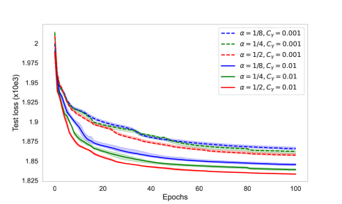
The effect of $C_{\gamma}$.

Figure 13 illustrates the convergence in both the squared gradient norm and the negative log-likelihood for $C_{\gamma}=0.001$ and $C_{\gamma}=0.01$ in Adagrad. In the case of the squared gradient norm, we have only plotted the results for $C_{\gamma}=0.001$ for better visualization, and the plot for $C_{\gamma}=0.01$ was already presented in Figure 3. It is clear that when $C_{\gamma}$ is set to 0.001, the convergence of the negative log-likelihood is slower. Similarly, the convergence in the squared gradient norm for $C_{\gamma}=0.001$ achieves convergence, but it is slower compared to the case of $C_{\gamma}=0.01$.


Refer to caption Refer to caption

Figure 13: IWAE on the CIFAR-10 Dataset with Adagrad for different values of $\alpha$ and $C_{\gamma}$. Bold lines represent the mean over 5 independent runs.

The Impact of Bias over Time.

Our experiments illustrate the negative log-likelihood with respect to epochs, and we observed that a higher value of $\alpha$ leads to faster convergence. The key point to consider when tuning $\alpha$ is that while convergence may be faster in terms of iterations, it may lead to higher computational costs. To illustrate this, we set a fixed time limit of 1000 seconds and tested different values of $\alpha$, plotting the test loss as a function of time in Figure 14. It is clear that with $\alpha=1/8$, the convergence is always slower, whereas choosing $\alpha=1/4$ achieves faster convergence than $\alpha=1/2$. While the difference may seem small here, with more complex models, the disparity becomes significant. Therefore, it is essential to tune the value of $\alpha$ to attain fast convergence and reduce computational time.


Refer to caption

Figure 14: Negative Log-Likelihood on the test set of the CIFAR-10 Dataset for IWAE with RMSProp for Different Values of $\alpha$ over time (in seconds). Bold lines represent the mean over 5 independent runs.

In this paper, all simulations were conducted using the Nvidia Tesla T4 GPU. The total computing hours required for the results presented in this paper are estimated to be around 50 to 100 hours of GPU usage.

Appendix C Some Examples of Biased Gradients

In this section, we explore examples of applications using biased gradient estimators while having control over the bias.

C.1 Self-Normalized Importance Sampling

Let $\pi$ be a probability measure on a measurable space $(\mathsf{X},\mathcal{X})$. The objective is to estimate $\pi(f)=\mathbb{E}_{\pi}[f(X)]$ for a measurable function $f:\mathcal{X}\rightarrow\mathbb{R}^{d}$ such that $\pi(|f|)<\infty$. Assume that $\pi(\mathrm{d}x)\propto w(x)\lambda(\mathrm{d}x)$, where $w$ is a positive weight function and $\lambda$ is a proposal probability distribution, and that $\lambda(w)=\int w(x)\lambda(\mathrm{d}x)<\infty$. For a function $f:\mathcal{X}\rightarrow\mathbb{R}^{d}$ such that $\pi(|f|)<\infty$, the identity

$$\pi(f)=\frac{\lambda(\omega f)}{\lambda(\omega)},$$ (8)

leads to the Self-Normalized Importance Sampling (SNIS) estimator:

$$\Pi_{N}f\left(X^{1:N}\right)=\sum_{i=1}^{N}\omega_{N}^{i}f\left(X^{i}\right),\quad\omega_{N}^{i}=\frac{w\left(X^{i}\right)}{\sum_{\ell=1}^{N}w\left(X^{\ell}\right)},$$

where $X^{1:N}=\left(X^{1},\ldots,X^{N}\right)$ are independent draws from $\lambda$ and the $\omega_{N}^{i}$ are called the normalized weights. Agapiou et al., (2017) shows that the bias of SNIS estimator can be expressed as:

$$\left\|\mathbb{E}\left[\Pi_{N}f\left(X^{1:N}\right)-\pi(f)\right]\right\|\leq\frac{12}{N}\frac{\lambda\left(\omega^{2}\right)}{\lambda(\omega)^{2}}.$$

This particular type of estimator can be found in the Importance Weighted Autoencoder (IWAE) framework (Burda et al.,, 2015), as illustrated in B. The estimator of the gradient of ELBO in IWAE corresponds to the biased SNIS estimator of the gradient of the marginal log likelihood $\log p_{\theta}(x)$. Consequently, based on these results, both the bias and Mean Squared Error (MSE) are of order $\mathcal{O}(1/k)$, where $k$ corresponds to the number of samples drawn from the variational posterior distribution.

C.2 Sequential Monte Carlo Methods

We focus here in the task of estimating the parameters, denoted as $\theta$, in Hidden Markov Models. In this context, the hidden Markov chain is denoted by $(X_{t})_{t\geq 0}$. The distribution of $X_{0}$ has density $\chi$ with respect to the Lebesgue measure $\mu$ and for all $t\geq 0$, the conditional distribution of $X_{t+1}$ given $X_{0:t}$ has density $m_{\theta}(X_{t},\cdot)$. It is assumed that this state is partially observed through an observation process $(Y_{t})_{0\leq t\leq T}$. The observations $Y_{0:t}$ are assumed to be independent conditionally on $X_{0:t}$ and, for all $0\leq t\leq T$, the distribution of $Y_{t}$ given $X_{0:t}$ depends on $X_{t}$ only and has density $g_{\theta}(X_{t},\cdot)$ with respect to the Lebesgue measure. The joint distribution of hidden states and observations is given by

$$p_{\theta}(x_{0:T},y_{0:T})=\chi(x_{0})g_{\theta}(x_{0},y_{0})\prod_{t=0}^{T-1}m_{\theta}(x_{t},x_{t+1})g_{\theta}(x_{t+1},y_{t+1}).$$

Our objective is to maximize the likelihood of the model:

$$p_{\theta}(y_{0:T})=\int p_{\theta}(x_{0:T},y_{0:T})\,\mathrm{d}x_{0:T}.$$

To use a gradient-based method for this maximization problem, we need to compute the gradient of the objective function. Under simple technical assumptions, by Fisher’s identity,

$\displaystyle\nabla_{\theta}\log p_{\theta}(y_{0:T})$ $\displaystyle=\int\nabla_{\theta}\log p_{\theta}(x_{0:T},y_{0:T})p_{\theta}(x_{0:T}|y_{0:T})\mathrm{d}x_{0:T}$
$\displaystyle=\mathbb{E}_{x_{0:T}\sim p_{\theta}(.|y_{0:T})}\left[\nabla_{\theta}\log p_{\theta}(x_{0:T},y_{0:T})\right]$
$\displaystyle=\mathbb{E}_{x_{0:T}\sim p_{\theta}(.|y_{0:T})}\left[\sum_{t=0}^{T-1}s_{t,\theta}\left(x_{t},x_{t+1}\right)\right],$

where $s_{t,\theta}\left(x,x^{\prime}\right)=\nabla_{\theta}\log\{m_{\theta}\left(x,x^{\prime}\right)g_{\theta}\left(x,y_{t+1}\right)\}$ for $t>0$ and by convention $s_{0,\theta}\left(x,x^{\prime}\right)=\nabla_{\theta}\log g_{\theta}\left(x,y_{0}\right)$. Given that the gradient of the log-likelihood represents the smoothed expectation of an additive functional, one may opt for Online Smoothing algorithms to mitigate computational costs. The estimation of the gradient $\nabla_{\theta}\log p_{\theta}(y_{0:T})$ is given by:

$$H_{\theta}\left(y_{0:T}\right)=\sum_{i=1}^{N}\frac{\omega_{T}^{i}}{\Omega_{T}}\tau_{T,\theta}^{i},$$

where $\{\tau_{T,\theta}^{i}\}_{i=1}^{N}$ are particle approximations obtained using particles $\{\left(\xi_{T}^{i},\omega_{T}^{i}\right)\}_{i=1}^{N}$ targeting the filtering distribution $\phi_{T}$, i.e. the conditional distribution of $x_{T}$ given $y_{0:T}$. In the Forward-only implementation of FFBSm (Del Moral et al.,, 2010), the particle approximations $\{\tau_{T,\theta}^{i}\}_{i=1}^{N}$ are computed using the following formula, with an initialization of $\tau_{0}^{i}=0$ for all $i\in\llbracket 1,N\rrbracket$:

$$\tau_{t+1,\theta}^{i}=\sum_{j=1}^{N}\frac{\omega_{t}^{j}m_{\theta}(\xi_{t}^{j},\xi_{t+1}^{i})}{\sum_{\ell=1}\omega_{t}^{\ell}m_{\theta}(\xi_{t}^{\ell},\xi_{t+1}^{i})}\left\{\tau_{t,\theta}^{j}+s_{t,\theta}(\xi_{t}^{j},\xi_{t+1}^{i})\right\},\quad t\in\mathbb{N}.$$

The estimator of the gradient $H_{\theta}\left(y_{0:T}\right)$ computed by the Forward-only implementation of FFBSm is biased. The bias and MSE of this estimator are of order $\mathcal{O}\left(1/N\right)$ (Del Moral et al.,, 2010), where $N$ corresponds to the number of particles used to estimate it. Using alternative recursion methods to compute $\{\tau_{T,\theta}^{i}\}_{i=1}^{N}$ results in different algorithms, such as the particle-based rapid incremental smoother (PARIS) (Olsson and Westerborn,, 2017) and its pseudo-marginal extension Gloaguen et al., (2022) and Parisian particle Gibbs (PPG) (Cardoso et al.,, 2023). In such cases, one can also control the bias and MSE of the estimator.

C.3 Policy Gradient for Average Reward over Infinite Horizon

Consider a finite Markov Decision Process (MDP) denoted as $(\mathcal{S},\mathcal{A},R,P)$, where $\mathcal{S}$ represents the state space, $\mathcal{A}$ denotes the action space, $R:\mathcal{S}\times\mathcal{A}\rightarrow\left[0,R_{\text{max}}\right]$ is a reward function, and $P$ is the transition model. The agent’s decision-making process is characterized by a parametric family of policies $\{\pi_{\theta}\}_{\theta\in\mathbb{R}^{d}}$, employing the soft-max parameterization. The reward function is given by:

$$V(\theta):=\mathbb{E}_{(S,A)\sim v_{\theta}}\left[\mathrm{R}(S,A)\right]=\sum_{(s,a)\in\mathcal{S}\times\mathcal{A}}v_{\theta}(s,a)\mathrm{R}(s,a),$$

where $v_{\theta}$ represents the unique stationary distribution of the state-action Markov Chain sequence $\left\{\left(S_{t},A_{t}\right)\right\}_{t\geq 1}$ generated by the policy $\pi_{\theta}$. Let $\lambda\in(0,1)$ be a discount factor and $T$ be sufficiently large, the estimator of the gradient of the objective function $V$ is given by:

$$H_{\theta}\left(S_{1:T},A_{1:T}\right)=\mathrm{R}\left(S_{T},A_{T}\right)\sum_{i=0}^{T-1}\lambda^{i}\nabla\log\pi_{\theta}\left(A_{T-i};S_{T-i}\right),$$

where $\left(S_{1:T},A_{1:T}\right):=\left(S_{1},A_{1},\ldots,S_{T},A_{T}\right)$ is a realization of state-action sequence generated by the policy $\pi_{\theta}$. It’s important to note that this gradient estimator is biased, and the bias is of order $\mathcal{O}(1-\lambda)$ (Karimi et al.,, 2019).

C.4 Zeroth-Order Gradient

Consider the problem of minimizing the objective function $V$. The zeroth-order gradient method is particularly valuable in scenarios where direct access to the gradient of the objective function is challenging or computationally expensive. The zeroth-order gradient oracle obtained by Gaussian smoothing (Nesterov and Spokoiny,, 2017) is given by:

$$H_{\theta}\left(X\right)=\frac{V(\theta+\tau X)-V(\theta)}{\tau}X,$$ (9)

where $\tau>0$ is a smoothing parameter and $X\sim\mathcal{N}(0,\mathit{I}_{d})$ a random Gaussian vector. Nesterov and Spokoiny, (2017, Lemma 3) provide the bias of this estimator:

$$\|\mathbb{E}\left[H_{\theta}\left(X\right)\right]-\nabla V\left(\theta\right)\|\leq\frac{\tau}{2}L(d+3)^{3/2}.$$ (10)

The application of these zeroth-order gradient methods can be found in generative adversarial networks (Moosavi-Dezfooli et al.,, 2017; Chen et al.,, 2017).