Beating one bit of Communication with Quantum Correlations in Smaller Dimensions

Abstract

As a consequence of Bell’s theorem, the statistics of measurements on some entangled states cannot be simulated with Local Hidden Variables (LHV) alone. The amount of communication that must be supplied is an intuitive quantifier of non-classicality. While it is obvious that this amount can be very large in general, it has been surprisingly difficult to find simple examples of quantum correlations, whose simulation requires more than one bit of communication. In this paper, we report the simplest example to date, which lives in the $(5,2,5,5)$ Bell scenario [the previously known smallest case living in the $(7,3,16,16)$ scenario]. The proof is built on the observation that the maximisation of the 1-bit score is equivalent to finding the best partition in which the sum of the local scores in the two sub-games is maximal.

I Introduction

Since Bell’s seminal theorem, we have known that the correlations made by some quantum systems cannot be reproduced solely with Local Hidden Variables (LHV) [1, 2]. Consequently, some have started asking how powerful are these quantum correlations in contrast to LHV, and compared to one another. One way to phrase this question is to ask how much additional resources are needed to supplement LHV in order to simulate these quantum correlations. Some have investigated the case for nonlocal boxes [3, 4, 5], but one resource that is most intuitive is classical communication, which we will be focusing on in this work.

Some works have been done on the average amount of communication needed to simulate the entanglement of a system of a generic dimension [6, 7, 8, 9]. On the other hand, going to a small, finite dimension, a substantial body of literature has been written on what could and could not be simulated with just a single bit of classical communication (1-bit). For two qubits, 1-bit is provably enough to simulate all the statistics of the maximally entangled state [6, 10, 11, 12, 13] and of a whole range of weakly-entangled states [14]; there is numerical evidence supporting the conjecture that all two-qubit states can be simulated with just 1-bit [15].

Conversely, some have tried to search for a correlation that could not be simulated by 1-bit. These correlations, or behaviors, can be sought for in Bell scenarios with $m_{A/B}$ inputs and $o_{A/B}$ outputs for Alice/Bob, denoted $(m_{A},m_{B},o_{A},o_{B})$. The set of 1-bit correlations forms a polytope, akin to the local polytope, but obviously includes signalling behaviours and is thus embedded in the full probability space. The real dimension of this space, called probability dimension, is given by $m_{A}m_{B}o_{A}o_{B}$ . Some have characterised these polytopes in the simplest scenarios, i.e. up to $(3,3,2,2)$, and found no violation by quantum correlations [17, 18, 19]. For larger scenarios, the task becomes computationally unfeasible. Using a different technique, Vértesi and Bene found a quantum correlation that is not simulatable with 1-bit, although it requires an infinite number of settings [20]. Eventually, just recently, Márton et al. found examples of quantum correlations that are not simulatable with 1-bit in finite scenarios [21]. Their constructions are based on parallel repetition. The smallest scenario in which they found examples are $(7,3,16,16)$ (probability dimension: 5376) for fixed-directional communication, and $(7,7,16,16)$ (probability dimension: 12544) or $(63,63,2,2)$ (probability dimension 15876) for bidirectional communication. In this work, we will present an example of a quantum correlation that is not simulatable with 1-bit for fixed directional communication, in the $(5,2,5,5)$ scenario (probability dimension: 250). The statistics of interest can be generated by suitable measurements on the maximally entangled state of two five-dimensional systems. This comes within the range of challenging but feasible experimental demonstrations [22, 23, 24, 25, 26, 27, 28, 29, 30, 31, 32, 33, 34, 35, 36, 37, 38].

The paper is structured as follows. In Section II we will first present a method to find the 1-bit bound that is faster than a brute force approach. In Section III we will present our Bell inequality and the corresponding correlation that lies outside the 1-bit polytope.

II Bell Inequalities for 1-bit of Communication

II.1 Defining the 1-bit polytope

Let us call the local set $\mathcal{L}$, the quantum set $\mathcal{Q}$, and the set of 1-bit communication strategies $\mathcal{L}_{+1}$. Like $\mathcal{L}$, $\mathcal{L}_{+1}$ is also a polytope, but one that spans outside the no-signalling space. Since it is a polytope, the maximum value of a linear inequality achieved by the set must be given by at least one of its extremum points. This simplifies the problem of finding the 1-bit bound into finding the extremum point which maximises the inequality.

Now let us call the set of inputs of Alice (Bob) as $\mathcal{X}\;(\mathcal{Y})$ with size $m_{A}$ ($m_{B}$) and her (his) outputs $\mathcal{A}\;(\mathcal{B})$ with size $o_{A}$ ($o_{B}$). The specific scenario of a game or inequality is denoted by the $(m_{A},m_{B},o_{A},o_{B})$ notation. In the usual studies of Bell nonlocality, the non-signalling constraints on $\mathcal{L}$ effectively reduce the dimension of the probability space under study to $m_{A}(o_{A}-1)m_{B}(o_{B}-1)+m_{A}(o_{A}-1)+m_{B}(o_{B}-1)$ [39]. However, the polytope $\mathcal{L}_{+1}$, however, is not bound by this constraint: we must work in the full probability space of dimension $m_{A}m_{B}o_{A}o_{B}$.

After receiving her input, Alice has $o_{A}^{m_{A}}$ possible deterministic strategies. She then has $\left(2^{m_{A}-1}-1\right)$ deterministic communication strategies. This number is given by Stirling’s number of the second kind, which gives the number of ways to partition a set into a fixed number of subsets. Finally, Bob has $o_{B}^{2m_{B}}$ possible deterministic strategies, where the two come from Alice’s bit of communication. This number can be reduced as there are duplicates, with the final number being

$$o_{A}^{m_{A}}\left(o_{B}^{m_{B}}+(2^{m_{A}-1}-1)(o_{B}^{2m_{B}}-o_{B}^{m_{B}})\right).$$

The number of extremum points grows very quickly with dimensions and direct facet enumeration is practically impossible once we go to (3,3,2,2), where some ingenious techniques are needed to enumerate the facets [19]. However, if we are given a Bell inequality, we could still find its 1-bit bound by running a brute force search on all the extremum points. Once we go above 20 million points or so, however, which is reached in (4,3,4,4), this also starts becoming unwieldy. This problem can be circumvented by noting that in order to find the maximum 1-bit bound of a Bell inequality, we do not need to find the Bell value of every single extremum point of $\mathcal{L}_{+1}$.

II.2 A faster computation for the 1-bit bound

A behaviour in a given scenario is given by a set of probabilities $p(a,b|x,y)$ for all $a,b,x,y$, which can be written as a vector. Similarly, a Bell inequality is given by a set of coefficients $V(a,b|x,y)$ for all $a,b,x,y$, which can also be written as a vector. As mentioned, the maximum score achieved by a polytope is obtained by at least one of its extremum points. Thus, the task of finding the 1-bit bound of a given Bell inequality $\vec{B}$ can be written as

$$\max_{\vec{p}\in\{\vec{p}_{\mathcal{L}_{+1},D}\}}{\vec{B}\cdot\vec{p}},$$ (1)

where $\{\vec{p}_{\mathcal{L}_{+1},D}\}$ is the set of extremum points of $\mathcal{L}_{+1}$. Each of the extremum points corresponds to a deterministic strategy. For each point, the output functions of Alice and Bob are given by $A(x)=\delta_{f(x),a}$ and $B(y,c)=\delta_{g(y,c),b}$, while the communication function is given by $C(x)=\delta_{h(x),c}$, for some assignment functions $f,g,h$ that assigns one value $a,b,c$ to every input combinations.

In a deterministic 1-bit communication strategy, Alice deterministically sends a 0 or 1 to Bob depending on her input. This means that Alice and Bob have agreed on a partitioning Alice’s inputs in two sets

$$\mathcal{J}=\{x\in\mathcal{X}|C(x)=0\}$$ (2)

and its complement $\mathcal{X}/\mathcal{J}$. When we consider the partitioned sub-strategies, they are local, as we have used the bit of communication. Thus, all deterministic 1-bit communication strategies can be decomposed into two local parts

$$\vec{p}_{\mathcal{L}_{+1},D}=\vec{p}_{\mathcal{L}^{\prime},D}^{\;\mathcal{J}}\oplus\vec{p}_{\mathcal{L}^{\prime\prime},D}^{\;\mathcal{X}/\mathcal{J}},$$ (3)

where $\oplus$ is the direct addition, $\mathcal{L}^{\prime}$ is the local polytope in the smaller scenario of $(|\mathcal{J}|,m_{B},o_{A},o_{B})$ and similarly for $\mathcal{L}^{\prime\prime}$. The two sub-strategies are local in their respective partitions and thus are extremum points of the local polytope in the smaller scenarios. Similarly, we can also partition $\vec{B}$ into two:

$$\vec{B}=\vec{B}^{\;\mathcal{J}}\oplus\vec{B}^{\;\mathcal{X}/\mathcal{J}}.$$ (4)

With these in mind, we can rewrite equation (1) in the following way:

$$\max_{\vec{p}\in\{\vec{p}_{\mathcal{L}_{+1},D}\}}{\vec{B}\cdot\vec{p}} =\max_{A(x),B(y,c),C(x)}{\vec{B}\cdot\vec{p}_{\mathcal{L}_{+1},D}}$$

$$=\max_{A(x),B(y,c),C(x)}{(\vec{B}^{\;\mathcal{J}}\oplus\vec{B}^{\;\mathcal{X}/\mathcal{J}})\cdot(\vec{p}_{\mathcal{L}^{\prime},D}^{\;\mathcal{J}}\oplus\vec{p}_{\mathcal{L}^{\prime\prime},D}^{\;\mathcal{X}/\mathcal{J}})}$$

$$=\max_{A(x),B(y,c),C(x)}\left(({\vec{B}^{\;\mathcal{J}}\cdot\vec{p}_{\mathcal{L}^{\prime},D}^{\;\mathcal{J}})+(\vec{B}^{\;\mathcal{X}/\mathcal{J}}\cdot\vec{p}_{\mathcal{L}^{\prime\prime},D}^{\;\mathcal{X}/\mathcal{J}})}\right)$$

$$=\max_{C(x)}\left(\max_{A^{\prime}(x),B(y,0)}({\vec{B}^{\;\mathcal{J}}\cdot\vec{p}_{\mathcal{L}^{\prime},D}^{\;\mathcal{J}})+\max_{A^{\prime\prime}(x),B(y,1)}(\vec{B}^{\;\mathcal{X}/\mathcal{J}}\cdot\vec{p}_{\mathcal{L}^{\prime\prime},D}^{\;\mathcal{X}/\mathcal{J}})}\right).$$ (5)

In the first equality, we rewrite the maximisation variables to be the strategies of the parties. In the second equality, we use equation (3) and (4). In the third equality, we partition the Bell vector along $\mathcal{J}$ and use the distributive property of the dot product and the direct sum. In the final equality, we note that the two terms are independent of each other, i.e., the local strategy of the first sub-inequality does not affect the score of the second sub-inequality. Thus, for a given partition $\mathcal{J}$, we can split the maximisation into two terms. Here, we write $A^{\prime}$ and $A^{\prime\prime}$ the strategies of Alice to denote that they are defined on the domain of the partitioned input sets. We can now also assign a value to the $c$ in the input arguments of $B$ since $c$ has a fixed value in each of the partitions as defined by equation (2).

For a more intuitive description, consider that for a given Bell game, a deterministic bit of communication allows the parties to effectively partition the game into two. One where her input falls in $\mathcal{J}$, and one where it does not. When she sends the bit to Bob, Bob now knows which partition of the game her input is in. In each of these partitions, they now play a normal Bell game. These two local strategies of the sub-games do not interact with each other, since the strategy in the first sub-game does not affect how they play and how they score in the second sub-game. Thus, a 1-bit strategy is optimum in the total Bell game if and only if its sub-strategies are also optimum in the sub-games. Thus, in order to find the maximum 1-bit strategy, one needs only to maximise the two sub-games using local deterministic strategies, for all the possible ways to partition the Bell game into two sub-games.

This rewritten maximisation can be run faster than the original form since finding the local bound of a game is a relatively fast task compared to enumerating over all 1-bit deterministic strategies. This speedup comes from the fact that when we rewrite this optimisation, we skip over the extremum points which are not optimum in the partitioned sub-games defined by the communication strategies. However, note that the result of the optimisation is still analytically exact, and this allows us to find the exact 1-bit bound in higher dimensions, which will be useful for the next sections.

III Finding quantum correlations that violate $\mathcal{L}_{+1}$

III.1 Five (and beyond) dimensional Bell-like inequalities for $\mathcal{L}_{+1}$

	$y=1$					$y=2$
$x=1$	1	$\cdot$	$\cdot$	$\cdot$	$\cdot$	1	$\cdot$	$\cdot$	$\cdot$	$\cdot$
	$\cdot$	1	$\cdot$	$\cdot$	$\cdot$	$\cdot$	1	$\cdot$	$\cdot$	$\cdot$
	$\cdot$	$\cdot$	1	$\cdot$	$\cdot$	$\cdot$	$\cdot$	1	$\cdot$	$\cdot$
	$\cdot$	$\cdot$	$\cdot$	1	$\cdot$	$\cdot$	$\cdot$	$\cdot$	1	$\cdot$
	$\cdot$	$\cdot$	$\cdot$	$\cdot$	1	$\cdot$	$\cdot$	$\cdot$	$\cdot$	1
$x=2$	1	$\cdot$	$\cdot$	$\cdot$	$\cdot$	$\cdot$	1	$\cdot$	$\cdot$	$\cdot$
	$\cdot$	1	$\cdot$	$\cdot$	$\cdot$	$\cdot$	$\cdot$	1	$\cdot$	$\cdot$
	$\cdot$	$\cdot$	1	$\cdot$	$\cdot$	$\cdot$	$\cdot$	$\cdot$	1	$\cdot$
	$\cdot$	$\cdot$	$\cdot$	1	$\cdot$	$\cdot$	$\cdot$	$\cdot$	$\cdot$	1
	$\cdot$	$\cdot$	$\cdot$	$\cdot$	1	1	$\cdot$	$\cdot$	$\cdot$	$\cdot$
$x=3$	1	$\cdot$	$\cdot$	$\cdot$	$\cdot$	$\cdot$	$\cdot$	1	$\cdot$	$\cdot$
	$\cdot$	1	$\cdot$	$\cdot$	$\cdot$	$\cdot$	$\cdot$	$\cdot$	1	$\cdot$
	$\cdot$	$\cdot$	1	$\cdot$	$\cdot$	$\cdot$	$\cdot$	$\cdot$	$\cdot$	1
	$\cdot$	$\cdot$	$\cdot$	1	$\cdot$	1	$\cdot$	$\cdot$	$\cdot$	$\cdot$
	$\cdot$	$\cdot$	$\cdot$	$\cdot$	1	$\cdot$	1	$\cdot$	$\cdot$	$\cdot$
$x=4$	1	$\cdot$	$\cdot$	$\cdot$	$\cdot$	$\cdot$	$\cdot$	$\cdot$	1	$\cdot$
	$\cdot$	1	$\cdot$	$\cdot$	$\cdot$	$\cdot$	$\cdot$	$\cdot$	$\cdot$	1
	$\cdot$	$\cdot$	1	$\cdot$	$\cdot$	1	$\cdot$	$\cdot$	$\cdot$	$\cdot$
	$\cdot$	$\cdot$	$\cdot$	1	$\cdot$	$\cdot$	1	$\cdot$	$\cdot$	$\cdot$
	$\cdot$	$\cdot$	$\cdot$	$\cdot$	1	$\cdot$	$\cdot$	1	$\cdot$	$\cdot$
$x=5$	1	$\cdot$	$\cdot$	$\cdot$	$\cdot$	$\cdot$	$\cdot$	$\cdot$	$\cdot$	1
	$\cdot$	1	$\cdot$	$\cdot$	$\cdot$	1	$\cdot$	$\cdot$	$\cdot$	$\cdot$
	$\cdot$	$\cdot$	1	$\cdot$	$\cdot$	$\cdot$	1	$\cdot$	$\cdot$	$\cdot$
	$\cdot$	$\cdot$	$\cdot$	1	$\cdot$	$\cdot$	$\cdot$	1	$\cdot$	$\cdot$
	$\cdot$	$\cdot$	$\cdot$	$\cdot$	1	$\cdot$	$\cdot$	$\cdot$	1	$\cdot$

Table 1: The coefficients of the Bell inequality in $(5,2,5,5)$. The table is written in full probability notation with the dots denoting zeros. The polytope bounds are $S_{\mathcal{L}}=6$ and $S_{\mathcal{L}_{+1}}=7$. The maximally entangled bipartite 6-dimensional states violate this with at least a score of $S_{\mathcal{Q}}=7.1777$.

Our first example comes as a generalisation of a previous correlation found in [15] to the $(5,2,5,5)$ scenario, shown in Table 1. This game is a truncated version of the XOR-d games for $d=5$ [40, 41, 42]. Up to some relabelling, the XOR-d games can be written as

$$\mathcal{I}_{d}(\mathcal{P})=\sum_{a,b,x,y}^{d-1}\left[a-b=xy\;\text{mod}\;d\right]P(a,b|x,y),$$ (6)

where $[\cdot]$ is the Iverson bracket, which evaluates to 1 when the expression inside is true and 0 otherwise. While $a,b,x,y$ usually runs from $\{0,1,...,d-1\}$, here we truncate $b$ to $\{0,1\}$.

This Bell inequality has local bound $S_{\mathcal{L}}=6$ and no-signalling bound $S_{\mathcal{NS}}=10$. More importantly, the 1-bit bound is $S_{\mathcal{L}_{+1}}$ = 7 while the quantum bound is in the range of $7.1777\leq S_{\mathcal{Q}}\leq 7.1788$, where the lower bound is obtained by an explicit example and the upper bound by the level 1+AB NPA hierarchy [43, 44]. The total dimension of the probability space of this scenario is 250, signifying an improvement from the previously reported smallest example for fixed directional communication: the (truncated, asymmetrised) two Magic squares found in [21] by method of parallel repetition feature the total dimension of 5376.

This can be further generalised to higher $d$. For example, the $d=6$ case in $(6,2,6,6)$ yields $S_{\mathcal{L}}=7$ , $S_{\mathcal{L}_{+1}}=8$, and $S_{\mathcal{NS}}=12$. The maximally entangled bipartite 6-dimensional states violate this with a score of $8.3173<S_{\mathcal{Q}}<8.3693$ (level 1+AB NPA). In general, for a $(d,2,d,d)$ scenario, $S_{\mathcal{L}}=d+1$, $S_{\mathcal{L}_{+1}}=d+2$, and $S_{\mathcal{NS}}=2d$.

III.2 Violating the inequality with quantum mechanics

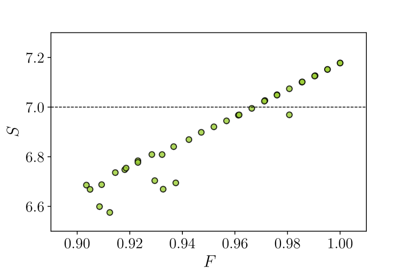
Figure 1: The plot shows the robustness of the violation against noise in the state. For each data point, we add Gaussian noise to the entries of $\rho=\ket{\Psi}\bra{\Psi}$ to get a noisy state and optimise the measurements numerically to obtain the maximum quantum score for that state. Since the optimisation is done heuristically, the points represent only a lower bound and sometimes the optimisation fails to converge on the global maximum, which gives the outliers. The fidelity of the noisy state ($F$) is the x-axis, while the score ($S$) is the y-axis. The dotted line is the local bound $S_{\mathcal{L}}$.

The lower bounds were obtained by numerical optimisation using MATLAB. All were obtained by fixing the state to the maximally entangled state

$$\ket{\Psi}=\frac{1}{\sqrt{d}}\sum_{i=0}^{d-1}\ket{ii},$$ (7)

where $d$ is the dimension of the output. The measurements are obtained numerically (link attached at the end), but we can still infer some patterns. Note that due to the nonlinear and heuristic nature of the optimisation, the precision and optimality of the resulting measurements are significantly limited. In the following inferences we will use the symbol $\simeq$ to denote a rough equality. In most cases, this rough equality is satisfied within a 10% margin, but in some cases, especially when the values are close to zero, this margin is not satisfied.

Let $\ket{a_{j}^{i}}\bra{a_{j}^{i}}$ $\Pi_{j}^{i}$ be Alice’s projector that corresponds to the $i$-th measurement and $j$-th output. The first observation is that, $\forall i\in\mathcal{X}$ and $\forall j,k\in\mathcal{A}$,

$$\left|\innerproduct{a_{j}^{i}}{a_{k}^{(i+1)\text{mod}d}}\right|^{2}\simeq\left|\innerproduct{a_{j}^{(i+1)\text{mod}d}}{a_{k}^{(i+2)\text{mod}d}}\right|^{2}.$$ (8)

I.e., the inner product between the $j$-th and $k$-th basis vectors from two ’neighbouring’ answers are always the same for every pair of ’neighbouring’ answers. Second, Bob’s two measurements form a mutually unbiased bases (MUB) with each other:

$$\left|\innerproduct{b_{i}^{1}}{b^{2}_{j}}\right|^{2}\simeq\frac{1}{d}.\quad\forall i,j\in\mathcal{B}.$$ (9)

Finally, the resulting behaviour is a convex combination of the nonlocal behaviour that maximally violates the inequality and white noise.

$$P(a,b|x,y)\simeq wP_{\mathcal{NS}}(a,b|x,y)+(1-w)\frac{1}{d^{2}},$$ (10)

where $P_{\mathcal{NS}}(a,b|x,y)=V(a,b|x,y)/d$, i.e., Table 1 reinterpreted as a non-signalling behaviour. For $d=5$, $w\simeq 0.64$ while for $d=6$, $w\simeq 0.63$.

Fig. 1 shows the heuristic quantum scores obtained by numerical optimisation for noisy states in $d=5$. A fidelity of around $\sim 0.97$ is required to observe a violation. This presents a possibility for a challenging, but doable, implementation using a high dimensional two-qudit state, such as those created in photonics, either using orbital angular momentum (OAM) [23, 24, 25, 26, 27], path [28, 29, 30, 31], time-bin [32, 33], frequency-bin [34, 35], or time-energy encoding [36, 37]. Recently, higher dimensional entanglement has even been demonstrated outside of photonics using trapped ions [38].

IV Conclusions

Here we have presented a family of quantum correlations for $d\geq 5$ which can not be simulated with a fixed directional communication from Alice to Bob with just a single bit of information. The $d=5$ case is, so far, the smallest example, both in the dimension of the quantum system and the total probability dimension, of a quantum correlation that cannot be simulated with a single bit of fixed directional communication from Bob. Indeed, even if Ref. [21] has examples with smaller output alphabets, the quantum realisations require higher-dimensional states. The small Hilbert space of this correlation presents a practical opportunity for an experimental implementation.

Our example can be extended for bidirectional communication by doing two of the games in parallel with reversed rules of Alice and Bob in the second game, resulting in a $(10,10,25,25)$ game. However, this does not improve on the two magic squares $(7,7,16,16)$ presented in [21].

V Code Availability

The measurements to obtain the lower bounds of $S_{\mathcal{Q}}$ can be found in https://github.com/PeterSidajaya/1-bit-part-deux.

VI Acknowledgements

This research is supported by the National Research Foundation, Singapore and A*STAR under its CQT Bridging Grant.

P.S. thanks Yeong-Cherng Liang, Swati Pandey, Kai-Siang Chen, and Gelo Noel M. Tabia for discussions and running some NPA hierarchy.

References

- Bell [1964] J. S. Bell, On the einstein podolsky rosen paradox, Physics Physique Fizika 1, 195 (1964).
- Scarani [2019] V. Scarani, Bell nonlocality (Oxford University Press, 2019).
- Popescu and Rohrlich [1994] S. Popescu and D. Rohrlich, Quantum nonlocality as an axiom, Foundations of Physics 24, 379 (1994).
- Brunner et al. [2005] N. Brunner, N. Gisin, and V. Scarani, Entanglement and non-locality are different resources, New Journal of Physics 7, 88 (2005).
- Brunner et al. [2008] N. Brunner, N. Gisin, S. Popescu, and V. Scarani, Simulation of partial entanglement with nonsignaling resources, Phys. Rev. A 78, 052111 (2008).
- Brassard et al. [1999] G. Brassard, R. Cleve, and A. Tapp, Cost of exactly simulating quantum entanglement with classical communication, Physical Review Letters 83, 1874 (1999).
- Massar et al. [2001] S. Massar, D. Bacon, N. J. Cerf, and R. Cleve, Classical simulation of quantum entanglement without local hidden variables, Physical Review A 63, 052305 (2001).
- Degorre et al. [2007] J. Degorre, S. Laplante, and J. Roland, Classical simulation of traceless binary observables on any bipartite quantum state, Phys. Rev. A 75, 012309 (2007).
- Brassard et al. [2019] G. Brassard, L. Devroye, and C. Gravel, Remote sampling with applications to general entanglement simulation, Entropy 21, 92 (2019).
- Steiner [2000] M. Steiner, Towards quantifying non-local information transfer: finite-bit non-locality, Physics Letters A 270, 239 (2000).
- Csirik [2002] J. A. Csirik, Cost of exactly simulating a bell pair using classical communication, Phys. Rev. A 66, 014302 (2002).
- Toner and Bacon [2003] B. F. Toner and D. Bacon, Communication cost of simulating bell correlations, Phys. Rev. Lett. 91, 187904 (2003).
- Degorre et al. [2005] J. Degorre, S. Laplante, and J. Roland, Simulating quantum correlations as a distributed sampling problem, Physical Review A 72, 062314 (2005).
- Renner and Quintino [2023] M. J. Renner and M. T. Quintino, The minimal communication cost for simulating entangled qubits, Quantum 7, 1149 (2023).
- Sidajaya et al. [2023] P. Sidajaya, A. D. Lim, B. Yu, and V. Scarani, Neural Network Approach to the Simulation of Entangled States with One Bit of Communication, Quantum 7, 1150 (2023).
- Note [1] Taking normalisation into account, the effective probability dimension is . We keep the formula in the main text to facilitate direct comparison with Ref. [21].
- Bacon and Toner [2003] D. Bacon and B. F. Toner, Bell inequalities with auxiliary communication, Phys. Rev. Lett. 90, 157904 (2003).
- Maxwell and Chitambar [2014] K. Maxwell and E. Chitambar, Bell inequalities with communication assistance, Phys. Rev. A 89, 042108 (2014).
- Zambrini Cruzeiro and Gisin [2019] E. Zambrini Cruzeiro and N. Gisin, Bell inequalities with one bit of communication, Entropy 21, 171 (2019).
- Vértesi and Bene [2009] T. Vértesi and E. Bene, Lower bound on the communication cost of simulating bipartite quantum correlations, Phys. Rev. A 80, 062316 (2009).
- Márton et al. [2023] I. Márton, E. Bene, P. Diviánszky, and T. Vértesi, Beating one bit of communication with and without quantum pseudo-telepathy, arXiv preprint arXiv:2308.10771 10.48550/arXiv.2308.10771 (2023).
- Erhard et al. [2020] M. Erhard, M. Krenn, and A. Zeilinger, Advances in high-dimensional quantum entanglement, Nature Reviews Physics 2, 365 (2020).
- Mair et al. [2001] A. Mair, A. Vaziri, G. Weihs, and A. Zeilinger, Entanglement of the orbital angular momentum states of photons, Nature 412, 313 (2001).
- Leach et al. [2010] J. Leach, B. Jack, J. Romero, A. K. Jha, A. M. Yao, S. Franke-Arnold, D. G. Ireland, R. W. Boyd, S. M. Barnett, and M. J. Padgett, Quantum correlations in optical angle–orbital angular momentum variables, Science 329, 662 (2010).
- Dada et al. [2011] A. C. Dada, J. Leach, G. S. Buller, M. J. Padgett, and E. Andersson, Experimental high-dimensional two-photon entanglement and violations of generalized bell inequalities, Nature Physics 7, 677 (2011).
- Krenn et al. [2014] M. Krenn, M. Huber, R. Fickler, R. Lapkiewicz, S. Ramelow, and A. Zeilinger, Generation and confirmation of a (100 100)-dimensional entangled quantum system, Proceedings of the National Academy of Sciences 111, 6243 (2014).
- Erhard et al. [2018] M. Erhard, R. Fickler, M. Krenn, and A. Zeilinger, Twisted photons: new quantum perspectives in high dimensions, Light: Science & Applications 7, 17146 (2018).
- Rossi et al. [2009] A. Rossi, G. Vallone, A. Chiuri, F. De Martini, and P. Mataloni, Multipath entanglement of two photons, Phys. Rev. Lett. 102, 153902 (2009).
- Schaeff et al. [2012] C. Schaeff, R. Polster, R. Lapkiewicz, R. Fickler, S. Ramelow, and A. Zeilinger, Scalable fiber integrated source for higher-dimensional path-entangled photonic qunits, Optics Express 20, 16145 (2012).
- Schaeff et al. [2015] C. Schaeff, R. Polster, M. Huber, S. Ramelow, and A. Zeilinger, Experimental access to higher-dimensional entangled quantum systems using integrated optics, Optica 2, 523 (2015).
- Wang et al. [2018] J. Wang, S. Paesani, Y. Ding, R. Santagati, P. Skrzypczyk, A. Salavrakos, J. Tura, R. Augusiak, L. Mančinska, D. Bacco, et al., Multidimensional quantum entanglement with large-scale integrated optics, Science 360, 285 (2018).
- Stucki et al. [2005] D. Stucki, H. Zbinden, and N. Gisin, A fabry–perot-like two-photon interferometer for high-dimensional time-bin entanglement, Journal of Modern Optics 52, 2637 (2005).
- Ikuta and Takesue [2016] T. Ikuta and H. Takesue, Enhanced violation of the collins-gisin-linden-massar-popescu inequality with optimized time-bin-entangled ququarts, Phys. Rev. A 93, 022307 (2016).
- Bernhard et al. [2013] C. Bernhard, B. Bessire, T. Feurer, and A. Stefanov, Shaping frequency-entangled qudits, Phys. Rev. A 88, 032322 (2013).
- Jin et al. [2016] R.-B. Jin, R. Shimizu, M. Fujiwara, M. Takeoka, R. Wakabayashi, T. Yamashita, S. Miki, H. Terai, T. Gerrits, and M. Sasaki, Simple method of generating and distributing frequency-entangled qudits, Quantum Science and Technology 1, 015004 (2016).
- Thew et al. [2004] R. T. Thew, A. Acín, H. Zbinden, and N. Gisin, Bell-type test of energy-time entangled qutrits, Phys. Rev. Lett. 93, 010503 (2004).
- Richart et al. [2012] D. Richart, Y. Fischer, and H. Weinfurter, Experimental implementation of higher dimensional time–energy entanglement, Applied Physics B 106, 543 (2012).
- Hrmo et al. [2023] P. Hrmo, B. Wilhelm, L. Gerster, M. W. van Mourik, M. Huber, R. Blatt, P. Schindler, T. Monz, and M. Ringbauer, Native qudit entanglement in a trapped ion quantum processor, Nature Communications 14, 2242 (2023).
- Collins and Gisin [2004] D. Collins and N. Gisin, A relevant two qubit bell inequality inequivalent to the chsh inequality, Journal of Physics A: Mathematical and General 37, 1775 (2004).
- Buhrman and Massar [2005] H. Buhrman and S. Massar, Causality and tsirelson’s bounds, Phys. Rev. A 72, 052103 (2005).
- Ji et al. [2008] S.-W. Ji, J. Lee, J. Lim, K. Nagata, and H.-W. Lee, Multisetting bell inequality for qudits, Phys. Rev. A 78, 052103 (2008).
- Liang et al. [2009] Y.-C. Liang, C.-W. Lim, and D.-L. Deng, Reexamination of a multisetting bell inequality for qudits, Phys. Rev. A 80, 052116 (2009).
- Navascués et al. [2008] M. Navascués, S. Pironio, and A. Acín, A convergent hierarchy of semidefinite programs characterizing the set of quantum correlations, New Journal of Physics 10, 073013 (2008).
- [44] N. Johnston, A. Cosentino, and V. Russo, Qetlab: Qetlab v0.9 10.5281/zenodo.44637.