Dilatonic Geometrodynamics of a Two-Dimensional Curved Surface due to a Quantum Mechanically Confined Particle

Abstract

We provide a unique and novel extension of da Costa’s calculation of a quantum mechanically constrained particle by analyzing the perturbative back reaction of the quantum confined particle’s eigenstates and spectra upon the geometry of the curved surface itself. We do this by first formulating a two dimensional action principle of the quantum constrained particle, which upon wave function variation reproduces Schrödinger’s equation including da Costa’s surface curvature induced potentials. Given this action principle, we vary its functional with respect to the embedded two dimensional inverse-metric to obtain the respective geometrodynamical Einstein equation. We solve this resulting Einstein equation perturbatively by first solving the da Costa’s Schrödinger equation to obtain an initial eigensystem, which is used as initial-input data for a perturbed metric inserted into the derived Einstein equation. As a proof of concept, we perform this calculation on a two-sphere and show its first iterative perturbed shape. We also include the back reaction of a constant external magnetic field in a separate calculation. The geometrodynamical analysis is performed within a two dimensional dilation gravity analog, due to several computational advantages.

I Introduction

Since da Costa’s, Jensen and Koppe’s seminal independent calculationsda Costa (1981); Jensen and Koppe (1971) demonstrating the emergence of curvature induced surface potentials within Schrödinger’s equation, the importance of differential geometric considerations in quantum semiconductor systems has spawned a wide plethora of exciting research areas. These curvature-induced surface potentials arise while expanding and separating the Laplace-Beltrami operator over $\mathbb{R}^{3}$ and confining a quantum particle to an embedded curved two dimensional surface $\mathcal{M}^{2}$. Taking $\mathcal{M}^{2}$ to the nanoscale opens a wide area of curvature induced quantum phenomena ranging from curved-spintronics, geometric nonlinear Hall effects, curvilinear magnetism, to strain-induced geometric potentials, to name a fewGentile et al. (2022). Additionally, the curvature of the nano surfaces, such as graphene nanotori, Buckyballs, diffusive ferromagnetic nanowires, etc., feeds back onto the quantum electronic material properties leading to an optimization and or tuning question/problemSalamone et al. (2022); Atanasov and Saxena (2010); Iorio and Lambiase (2014); de Lima et al. (2021); Gomes Silva et al. (2020); Ma et al. (2022).

Now, since the da Costa paradigm (which generalizes Jensen and Koppe’s work to arbitrary $\mathcal{M}^{2}$) necessitates differential geometric considerations in quantum systems, it sets the stage for holographic, analog-gravity, wormhole and black hole dual description extensions for two dimensional nanoscale semiconductors and materialsSchmidt and Pereira (2023); Atanasov (2020); Duenas-Vidal and Segovia (2023); Alencar et al. (2021); de Souza et al. (2022); Biswas and Ghosh (2020); Costa Filho et al. (2021); Zali and Sadeghi (2020); Meschede et al. (2023). This stringy-pathway also provides a unique, novel and previously unexplored way to address an important aforementioned question about geometric shape optimization for curved two dimensional semiconductor devicesGentile et al. (2022). This is the premise of our work in this manuscript.

The important question of shape optimization and perturbative shape evolution of semiconductor devices due to external fields and/or quantum mechanical processes on their surfaces has been of great interest in the above mentioned and many other related research fieldsRodriguez et al. (2020); Solin et al. (2000); Moussa et al. (2003); Pugsley et al. (2013); Moussa et al. (2001); Otomori et al. (2015); Yamada et al. (2010). The specific proposed premise of this paper is to think about confining a quantum mechanical particle to the two dimensional surface of a curved semiconductor or nano device (such as a Buckyball/carbon-nanotube, etc.) and analyze how the particles’ resulting eigensystem feeds back onto the geometry of the curved surface. In other words, is there an optimized nano-geometry for a given quantum particle to be confined to, which would represent the total system’s lowest eigenenergy configuration and therefore minimize any externally required work for confinement. Knowledge of such optimized geometries would then have significant application in device design and manufacturing.

Our preliminary results demonstrate there is a quantum confined eigensystem feedback which generates geometric deformations (a geometric strain of some kind) of the original chosen two dimensional semiconductor surface. It thus becomes an important task to compute these deformations in order to discover, or perturbatively narrow down, the ideal optimized geometric shape for the two dimensional curved surface. Additionally, in the presence of external fields, such as electromagnetic fields, the geometric deformations on the semiconductor attain additional complications with rich physics. The full geometrodynamics of this rich physical scenario turns out to be fully captured by a dual two dimensional dilaton gravity, nearly identical to the two dimensional quantum gravities that arise in the near horizon of four dimensional classical black holes.

Our starting point is the seminal work of da Costa da Costa (1981), who showed that for a particle quantum mechanically confined to a two dimensional curved surface embedded in $\mathbb{R}^{3}$, the pullback of Schrödinger’s equation results in the appearance of surface potentials that depend on the two dimensional curved surface’s Ricci scalar and also the extrinsic curvature. Thus, motivated by the finite element method, formulating a two dimensional action principle of the quantum constrained particle, which upon wave function variation reproduces Schrödinger’s equation according to da Costa, provides us with a foundational starting point to a full geometrodynamical description of this physical scenario.

Let $\vec{R}$ be the position vector of any point $Q$ $\in$ $\mathbb{R}^{3}$, such that $\vec{R}=\vec{R}(x,y,z)$. Next, $\vec{r}=\vec{r}(\theta,\phi)$ is the locus of points of a curved two dimensional surface $\mathcal{M}^{2}$, embedded in $\mathbb{R}^{3}$. To reach $Q$ from $\mathcal{M}^{2}$ we choose a perpendicular distance $\rho$ from $\mathcal{M}^{2}$ to $Q$. Thus $\vec{R}=\vec{r}+\rho\hat{n}$, where $\hat{n}$ is the unit normal to $\mathcal{M}^{2}$. We will define the three dimensional Euclidean metric in the usual way:

$$g_{\mu\nu}=\left(\partial_{\mu}\vec{R}\right)\cdot\left(\partial_{\nu}\vec{R}\right),$$ (1)

and the metric on $\mathcal{M}^{2}$ (first fundamental form) given by:

$$h_{ab}=\left(\partial_{a}\vec{r}\right)\cdot\left(\partial_{b}\vec{r}\right).$$ (2)

Here, greek indices range over the three cartesian coordinates and latin indices range over the two embedded curved coordinates. We also define the extrinsic curvature (second fundamental form) given by:

$$k_{ab}=\left(\partial_{a}\vec{r}\right)\cdot\left(\partial_{b}\hat{n}\right),$$ (3)

which depends on how $\vec{r}$ is embedded in $\mathbb{R}^{3}$ and informs about the rate of change of $\hat{n}$ as it is parallel transported across $\mathcal{M}^{2}$.

Now, given the above definitions and quoting results from [da Costa, 1981], the determinant $g=\det\left(g_{\mu\nu}\right)$ can be shown to take the form:

$$g=h\left(1+\rho\mathcal{K}+\rho^{2}\mathcal{R}/2\right)^{2},$$ (4)

where $h$ is the determinant of $h_{ab}$, $\mathcal{K}$ is the trace of the extrinsic curvature and $\mathcal{R}$ is the Ricci scalar curvature (twice the Gaussian curvature) of $\mathcal{M}^{2}$. Now considering this result and the three dimensional steady state Schrödinger equation:

$$-\frac{\hbar^{2}}{2m}\frac{1}{\sqrt{g}}\partial_{\mu}\left(\sqrt{g}g^{\mu\nu}\partial_{\nu}\psi\right)+V_{0}\tilde{\delta}(\rho)\psi=E\psi,$$ (5)

where $\tilde{\delta}(r)$ is an anti-Dirac delta-function such that $V(\rho)=V_{0}\tilde{\delta}(\rho)$ confines the particle to the two dimensional surface, i.e.

$$\tilde{\delta}(\rho)=\begin{cases}0&\rho=0\\ \infty&\rho\neq 0\end{cases},$$ (6)

we are able to separate the three dimensional equation (5) into two equations via the ansatz $\psi=\psi_{2D}(\theta,\phi)R(\rho)$ yielding da Costa (1981):

$$-\frac{\hbar^{2}}{2m}\frac{1}{\sqrt{h}}\partial_{a}\left(\sqrt{h}h^{ab}\partial_{b}\psi_{2D}\right)+$$

$$-\frac{\hbar^{2}}{2m}\left\{\left(\mathcal{K}/2\right)^{2}-\mathcal{R}/2\right\}\psi_{2D}=E_{2D}\psi_{2D}$$ (7)

$$-\frac{\hbar^{2}}{2m}R^{\prime\prime}+V_{0}\tilde{\delta}(\rho)R=E_{\rho}R.$$ (8)

II Two Dimensional Gravity Duality

The main computational tool we implement to solve derived and given field equations is rooted in the finite element analysis within the framework of the action integral principle Ram-Mohan (2002). In this paradigm, device geometry is discretized into refined finite element meshes. Within each element, potential functions are expressed as linear combination of Hermite interpolation polynomials multiplied by as-yet undetermined coefficients. Employing the principle of stationary action, variation of the action integral with respect to these undetermined coefficients results in a set of linear equations, which are then solved using sparse matrix solvers.

Thus, our first task is to construct an action whose equation of motion is given by (7) after functional variation with respect to $\psi_{2D}$. Assuming, without loss of generality, that $\psi_{2D}$ is real as this does not affect the final version of Schrödinger’s equation in (7), we have the obvious choice given by:

$$\begin{split}S=&\frac{\hbar^{2}}{4m}\int d^{2}x\sqrt{h}\\ &\left\{\partial_{a}\psi_{2D}\partial^{a}\psi_{2D}+\left[\mathcal{R}/2-\left(\mathcal{K}/2\right)^{2}\right]\psi_{2D}^{2}-\epsilon\psi_{2D}^{2}\right\},\end{split}$$ (9)

where $\epsilon$ is the scaled dimensionless energy $E_{2D}$. The above action can now be employed via the finite element analysis method to solve the Schrödinger equation (7) in order to compute eigenstates and eigenvalues for a plethora of differing curved two dimensional geometries. However, what is previously unexplored and one of the major research insights of this paper, is that the above action can be utilized to explore shape optimization of the two dimensional embedded semiconductor surface via a metric variation with respect to $h_{ab}$. In other words, we are the first to formulate a full geometrodynamical description of the back reaction of the confined quantum particle’s eigensystem onto the embedded curved surface, by computing the respective Einstein equation of the action given above in (9).

The respective Einstein equation of (9) will be given by the variation with respect to the embedded curved surface’s inverse metric (for canonical reasons) $h^{ab}$. However, before performing this variation, it is a very useful task to rescale the wave function in terms of a dilaton field $\varphi$, given by $\psi=e^{-\varphi}$. This rescaling improves and simplifies the very lengthy calculation of the respective Einstein equation. Given this rescaling, the action (9) takes the form:

$$S=\frac{\hbar^{2}}{4m}\int d^{2}x\sqrt{h}e^{-2\varphi}\left\{\partial_{a}\varphi\partial^{a}\varphi+\mathcal{R}/2-\mathcal{K}^{2}/4-\epsilon\right\}.$$ (10)

At this point we should pause and comment on how conveniently and surprisingly the above action for a quantum particle confined to a two dimensional curved surface is analogously described by a two dimensional dilaton gravity, which traditionally arises when describing horizon degrees of freedom of four dimensional black holes. For comparison, the two dimensional theory that arises in the near horizon of a charged spherically symmetric (Reissner-Nördstrom) black hole is given by:

$$\begin{split}&S_{2D}^{RN}=\\ &\frac{\ell^{2}}{4G}\int d^{2}x\sqrt{-g}e^{-2\varphi}\left\{2\partial_{a}\varphi\partial^{a}\varphi+\mathcal{R}-GF^{2}+\frac{2e^{2\varphi}}{\ell^{2}}\right\},\end{split}$$ (11)

where $G$ is Newton’s gravitational constant, $\ell$ is the two dimensional $AdS$ radius and $F$ is the two dimensionally reduced electromagnetic curvature two form.

When comparing the above two actions, (10) and (11), an immediate duality is evident which we summarize in the ‘da Costa/2D dilaton Gravity’ dictionary of Table 1.

Table 1: Dictionary of da Costa’s 2D quantum confined objects (quantities) and their corresponding duals in 2D dilaton gravity.

da Costa’s 2D Curved Confined Quantum Particle		Two Dimensional Near-Horizon Black Hole Dilaton Gravity
$\ell$	two dimensional $AdS$ radius	$\hbar$	Planck’s constant
$m$	confined particle mass	$G$	Newton’s Gravitational Constant
$\varphi$	logarithm of the quantum wave function	$\varphi$	gravitational dilaton scale of the $S^{2}$ factor
$h_{ab}$ $(h)$	Euclidian 2D curved embedded metric	$g_{ab}$ $(-g)$	$s$-wave near-horizon dimensionally reduced black hole
$\mathcal{R}$	semiconductor surface Ricci scalar curvature	$\mathcal{R}$	near-horizon 2D spacetime Ricci scalar curvature
$\mathcal{K}^{2}/4$	modulo semiconductor surface intrinsic curvature squared	$GF^{2}$	modulo internal Maxwell tensor squared
$\epsilon$	unitless energy eigenvalue	$\frac{2e^{2\varphi}}{\ell^{2}}$	cosmological term

Next, given the above duality we proceed to calculate the geometrodynamical Einstein equation of (10) via variation with respect to the inverse two dimensionally curved inverse metric $h^{ab}$. This derivation of the Einstein equation is in general non-trivial, mainly due to the overall $e^{-2\varphi}$ dilatonic weight in the action. This weight in conjunction with Hamilton’s principle does not allow us to drop Ricci tensor variations as boundary terms, as one would in the Einstein-Hilbert action principle of four dimensional general relativity. In stead, terms of the order $\delta R_{ab}$ contribute to the final Euler-Lagrange equations of motion. Specifically, our Einstein equation of motion relies on the following properties of the variation of the Riemann tensor and Levi-Civita connection in any dimension:

$$\begin{split}\delta R\indices{{}^{a}_{b}{}_{m}{}_{n}}=&\nabla_{m}\delta\Gamma\indices{{}^{a}_{b}{}_{n}}-\nabla_{n}\delta\Gamma\indices{{}^{a}_{b}{}_{m}}\\ \delta\Gamma\indices{{}^{a}_{m}{}_{n}}=&\frac{1}{2}\left(-h_{dn}\nabla_{m}\delta h^{ad}-h_{dm}\nabla_{n}\delta h^{ad}\right.\\ &\left.+h_{sm}h_{dn}\nabla^{a}\delta h^{sd}\right).\end{split}$$ (12)

Additionally we note that the Einstein tensor:

$$\begin{split}R_{ab}-\frac{1}{2}g_{ab}\mathcal{R}=0\end{split}$$ (13)

is identically zero for any Riemann surface in two dimensions, thus all embedded $h_{ab}$’s are Einstein manifolds. After very extensive and lengthy calculation, we obtain the following final result for the variation of (10) with respect to $h^{ab}$:

$$\begin{split}&\left\{-\frac{1}{2}h_{ab}\left(\partial_{c}\varphi\partial^{c}\varphi-\frac{\mathcal{K}^{2}}{4}-\epsilon\right)+\partial_{a}\varphi\partial_{b}\varphi-\frac{1}{2}\mathcal{K}k_{ab}\right\}e^{-2\varphi}\\ &+\frac{1}{2}\left(h_{ab}\square e^{-2\varphi}-\nabla_{a}\nabla_{b}e^{-2\varphi}\right)=0.\end{split}$$ (14)

The above can be simplified without loss of generality in two dimensions by tracing and thus yielding one single geometrodynamical Einstein equation, given by:

$$-\mathcal{K}^{2}/4+\epsilon+2\nabla_{a}\varphi\nabla^{a}\varphi-\square\varphi=0.$$ (15)

This result (15) in conjunction with (7) provides a full quantum mechanical and geometrodynamical description of the da Costa’s quantum confined particle.

III Geometric Optimization: A Single Iterative Perturbative Solution

As proposed above we are interested in using (7) and (15) as a powerful tool for the study of shape optimization in this particular physical scenario. A full iterative perturbative approach using finite element analysis and including external fields, is outlined in detail in the flowchart depicted in Fig. 1.

Figure 1: Flowchart of an iterative perturbative shape optimization using (7) and (15), assuming convergence.

However as a proof of concept and for the sake of analyticity, our initial approach here will follow a first iterative perturbative outline given by:

• First we select a specific two dimensional curved surface. Surfaces that are of interest in this area of study include the two sphere and the two torus da Silva et al. (2017); Ferrari and Cuoghi (2008); Schmidt (2019) among others. We will chose the two sphere for analytical reasons.

• We then proceed to solve (7) thereby obtaining an initial eigensystem, i.e. $\left(\varphi_{n}^{0},\epsilon_{n}^{0}\right)$. As aforementioned for the two sphere, the initial eigensystem is obtained analytically and given by spherical harmonics.

• Next, we introduce a perturbation to the initially chosen geometry. For example, choosing a two sphere with metric given by:

  $$h_{ab}=\left(\partial_{a}\vec{r}\right)\cdot\left(\partial_{b}\vec{r}\right)=\left(\begin{array}[]{cc}1&0\\ 0&\sin^{2}\theta\end{array}\right)$$ (18)

  a simple and general perturbation, to $\mathcal{O}(\lambda^{3})$, in the radial direction is given by:

  $$\begin{split}h_{ab}^{pert}={\left(\begin{array}[]{cc}\left(\alpha+\lambda F\right)^{2}+\lambda^{2}\left(\partial_{\theta}F\right)^{2}&\lambda^{2}\left(\partial_{\theta}F\right)\left(\partial_{\phi}F\right)\\ \lambda^{2}\left(\partial_{\theta}F\right)\left(\partial_{\phi}F\right)&\left(\alpha+\lambda F\right)^{2}\sin^{2}\theta+\lambda^{2}\left(\partial_{\phi}F\right)^{2}\end{array}\right)}.\end{split}$$ (19)

  for some small perturbation parameter $\lambda$, arbitrary scale parameter $\alpha$ and unknown function $F(\theta,\phi)$.

• The next step is to take $\left(\varphi_{n}^{0},\epsilon_{n}^{0}\right)$ and $h_{ab}^{pert}$ and insert them into the traced Einstein equation (15) for a given $n$ value, thereby obtaining a partial differential equation for $F(\theta,\phi)$ and foraging for an analytical solution for the given perturbation.

• We then end by demonstrating a plot of the this first iterative perturbative shape optimization of $\mathcal{M}^{2}$, due to a quantum confined particle.

In addition to the above outline and flow chart, a full simultaneous numerical solution via the finite element analysis paradigm of (7) and (15) is currently under investigation by our research collaboration for near future forthcoming work, to provide an instant numerical geometric optimization for $\mathcal{M}^{2}$ due to quantum confinement.

III.1 The $s$-wave Case

As mentioned above, choosing the two sphere as our initial geometry for $\mathcal{M}^{2}$ and setting $\epsilon=-l(l+1)$ in (9), results in spherical harmonics, $Y_{l}^{m}(\theta,\phi)$ where $n\to(l,m)$, as our initial eigensystem. Feeding the above into (15) and solving in the $s$-wave scenario ($l=m=0$) and assuming only $\theta$ dependence in the perturbation function $F$ in (19), yields the following analytical solution to $\mathcal{O}(\lambda^{2})$:

$$\begin{split}&F(\theta)=\alpha\left[\frac{1}{2}+\beta\cos{\theta}\right.\\ &\left.+\gamma\left(-1+\cos{\theta}\left(-\frac{1}{2}\ln{\left(1-\cos{\theta}\right)}+\frac{1}{2}\ln{\left(1+\cos\theta\right)}\right)\right)\right],\end{split}$$ (20)

where $\beta$ and $\gamma$ are integration constants. The integration constants should be dependent upon semiconductor material properties, such as modulus, stress, strain, conductive properties, etc. We have not included those type of contributions in our theoretical frame work as of yet, and thus, we will choose values for $\alpha$, $\beta$ and $\gamma$ that provide finite solutions to first iteration with respect to the flow chart in Fig. 1, that are scalable to a perturbed unit sphere for proof of concept.

For the $s$-wave case, we have identified three finite interesting cases depicted in Fig. 2-4 below. For each figure, we implemented the perturbation solution (LABEL:eq:swFf) and plotted the resulting perturbed two sphere. The three cases included values for $\alpha$, $\beta$ and $\gamma$ that range between 0 and 1. The specific choice of $\alpha$ is determined in order to compare our plots to that of a unit two sphere for visualization purposes. The first case in Fig. 2, $\beta$ and $\gamma$ are positive and equal; for the second case in Fig. 3, $\beta$ and $\gamma$ are of opposing sign and equal in magnitude; and in the third case, Fig. 4, the values for $\beta$ and $\gamma$ differ by a factor of 10.

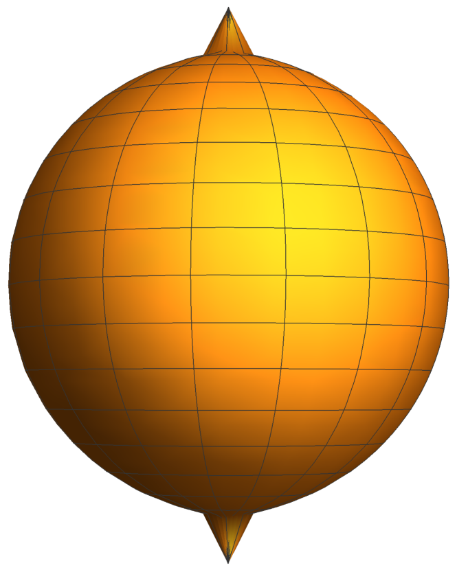
(a)

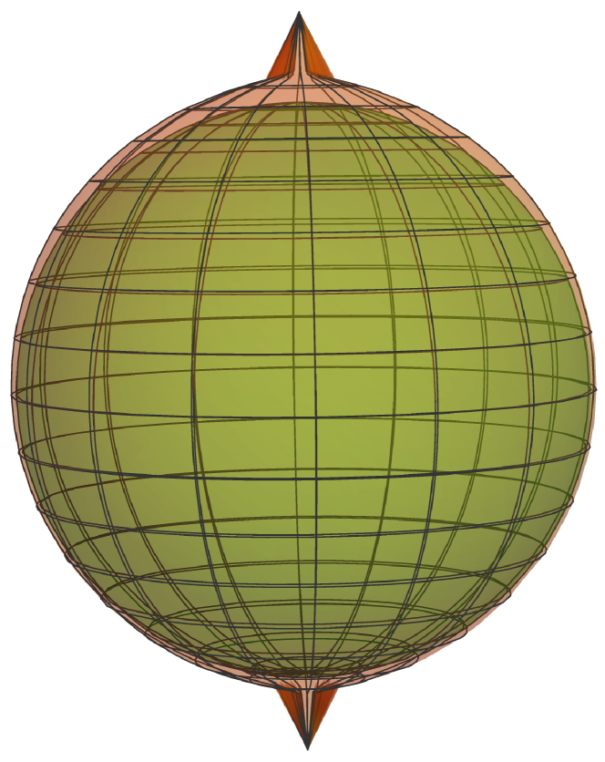
(b)

Figure 2: Perturbed geometry 2(a) due to a quantum confined particle a la da Costa, and comparison to initial unperturbed geometry (green) 2(b). The values for $\beta$ and $\gamma$ are positive, equal and bounded between 0 and 1.

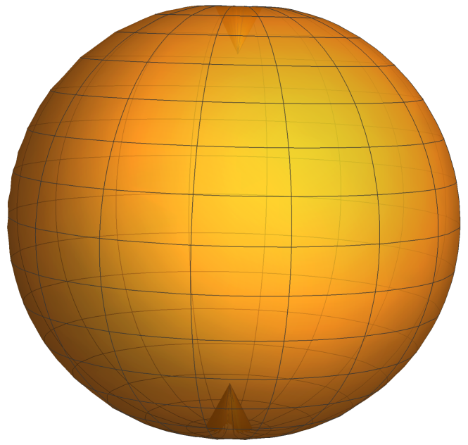
(a)

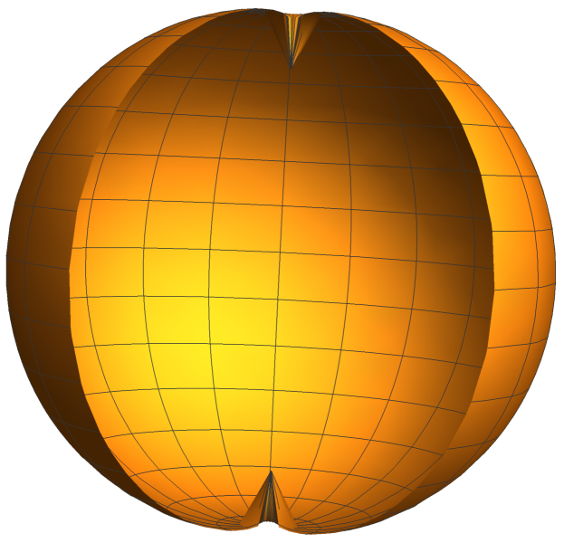
(b)

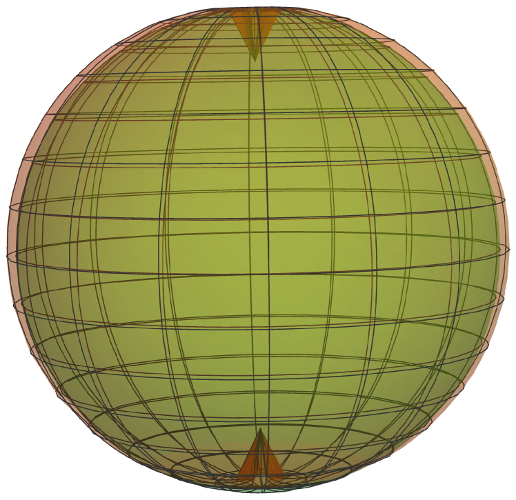
(c)

Figure 3: Perturbed geometry 3(a) and its cross sectional plot 3(b) (displaying the interior) due to a quantum confined particle a la da Costa, and comparison to initial unperturbed geometry (green) 3(c). The values for $\beta$ and $\gamma$ are opposite in sign, equal in magnitude and bounded between 0 and 1.

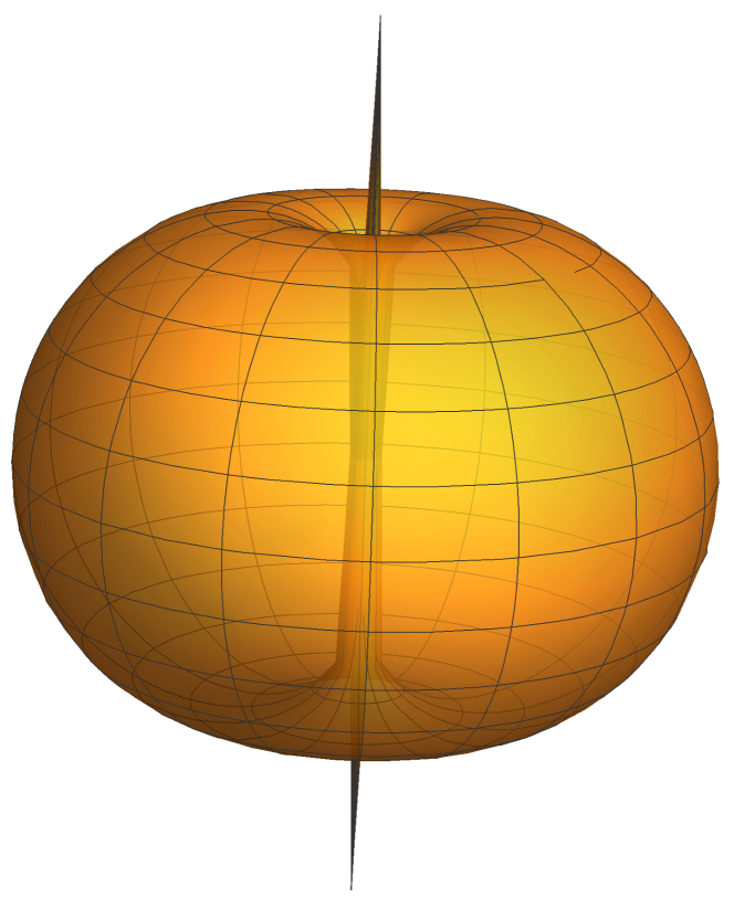
(a)

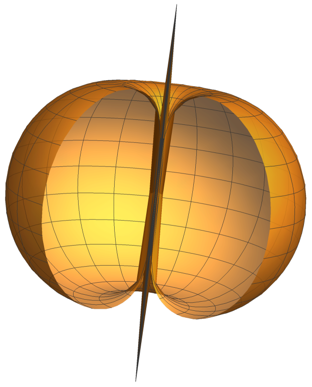
(b)

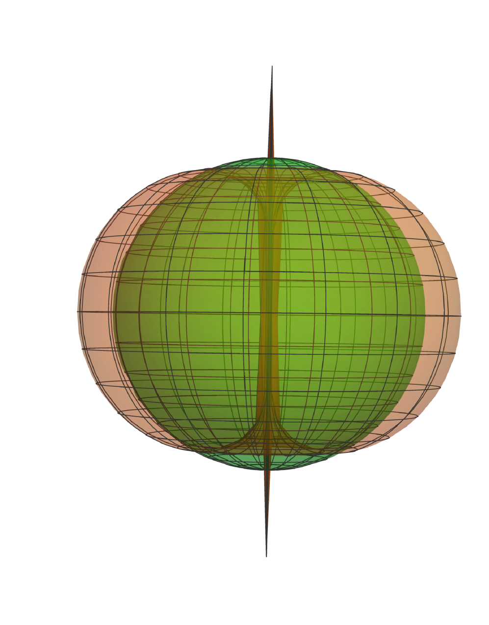
(c)

Figure 4: Perturbed geometry 4(a) and its cross sectional plot 4(b) (displaying the interior) due to a quantum confined particle a la da Costa, and comparison to initial unperturbed geometry (green) 4(c). The values for $\beta$ and $\gamma$ are opposite in sign, differ by a factor of 10 in magnitude and bounded between 0 and 1.

From the above mentioned figures it is apparent that there is a geometrodynamical feedback from the quantum confined particle’s eigensystem onto the initially chosen geometry of $\mathcal{M}^{2}$. We have made specific choices to make the geometric deformations visible, but it is still an ongoing investigation on tuning these parameters to actual material science properties of specific nano-semiconductors.

III.2 The $l=1$ and $m=\pm 1$ Cases

Two of the $l=1$ cases are another scenario where we are able to obtain analytical solutions for the perturbation function $F$, assuming only $\theta$ dependence and following the same procedures from the previous subsection III.1. For the $m=0$ case, we were not able to find a closed form analytical solution, but the other two cases $m=\pm 1$, there exists one common and unique analytical closed form solution in terms of Legendre polynomials ($P_{n}(x)$) and Legendre functions of the second kind ($Q_{n}(x)$), given by:

$$\begin{split}F(\theta)=&\alpha\left[2+\alpha^{2}+\beta P_{(-1+\sqrt{33})/2}(\cos\theta)\right.\\ &\left.+\gamma Q_{(-1+\sqrt{33})/2}(\cos\theta)\right].\end{split}$$ (21)

For this specific case, we display two sets of plots for choices of the scale parameter $\alpha$ and integration constants $\beta$ and $\gamma$. In the first plot, displayed in Fig. 5, the integration constants are equal and between 0 and 1. Varying the constants in sign only affects the direction of the polar peaks along the $z$-axis. The overall pumpkin shape seems universally unaffected. In Fig. 6 the integration constants differ by a factor of 10, but still sampled between 0 and 1. Both perturbed geometries are compared to a green unit two sphere in the second plot of each case.

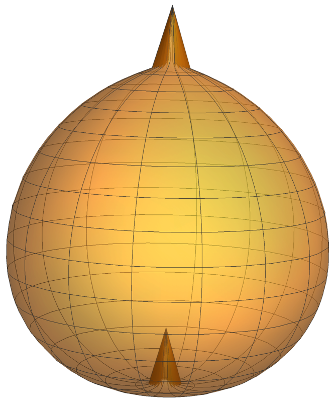
(a)

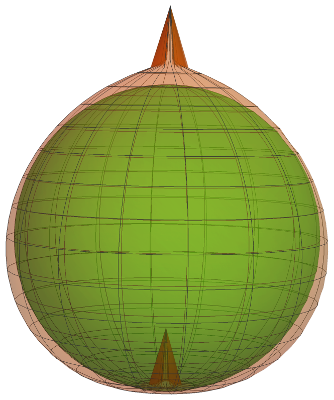
(b)

Figure 5: Perturbed geometry 5(a) due to a quantum confined particle a la da Costa, and comparison to initial unperturbed (green) geometry 5(b). The values for $\beta$ and $\gamma$ are positive, equal and bounded between 0 and 1.

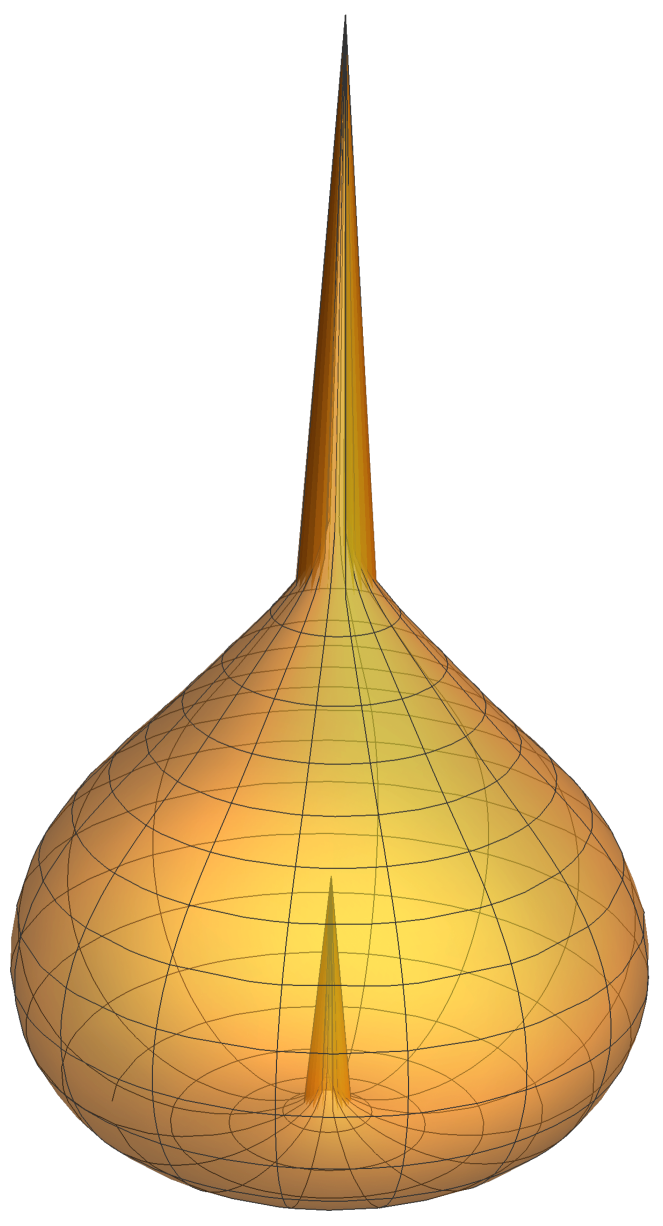
(a)

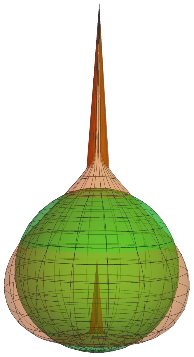
(b)

Figure 6: Perturbed geometry 6(a) due to a quantum confined particle a la da Costa, and comparison to initial unperturbed geometry 6(b). The values for $\beta$ and $\gamma$ are positive, differ by a factor of 10 and bounded between 0 and 1.

IV External Fields

Finally and as proposed above, we will detail and outline how to incorporate the presence of external electromagnetic fields in our formalism of geometric shape optimization. The presence of external fields is very important, since they can be used to tune desired outcomes and or appear naturally due to electronic devices/designs. However, our unique dual description allows us to unveil new phenomena and rich physics, that has to-date eluded the majority of researchers in this field. This is mainly due to our action integral approach, motivated from the finite element analysis paradigm, and resulting gravity analog detailed in Table 1. To begin, let us start by outlining a simple example of a unit two sphere centered at the origin with an external constant magnetic field along the $z$-axis, i.e.:

$$\begin{split}h_{ab}=&\left(\begin{array}[]{cc}1&0\\ 0&\sin^{2}\theta\end{array}\right)~{}\text{and}\\ \vec{B}=&B_{0}\hat{k}.\end{split}$$ (22)

One choice for a three vector potential whose curl yields the above magnetic field is given by:

$$\vec{A}= -B_{0}y\hat{\imath}.$$ (23)

Now, to incorporate this external magnetic field in da Costa’s (7), we need to first augment the operator $\partial_{a}$ by the pullback of $\vec{A}$ given by $A_{a}=\partial_{a}\vec{r}\cdot\vec{A}$ and thus defining the gauge covariant derivative, in the usual way, on the two dimensional curved surface: $D_{a}=\nabla_{a}-ieA_{a}$.

This is standard practice in the respective research field, but what has not been addressed before (until now in this work), is the fact that pulling down the three vector $\vec{A}$ to the two dimensional curved surface also induces a circulating surface magnetic field sourced by antiparallel surface currents, projected and distributed nontrivially on the respective embedded curved surface. Let us demonstrate; first, the pullback of the three vector potential in the above simple example gives rise to the embedded electromagnetic field tensor (curvature two form) given by:

$$\begin{split}F_{ab}=&\partial_{a}A_{b}-\partial_{b}A_{a}=\left(\begin{array}[]{cc}0&-B_{\theta}\\ B_{\theta}&0\end{array}\right)\\ =&\left(\begin{array}[]{cc}0&-B_{0}\cos\theta\sin\theta\\ B_{0}\cos\theta\sin\theta&0\end{array}\right)\end{split}$$ (24)

which (keeping in mind that $F_{ab}$ is purely spacial) reveals the induced embedded two dimensional specially dynamic magnetic field. The source of this induced magnetic field is a current density nontrivially distributed across the curved two dimensional surface, depicted in Fig. 8, which can be determined by the Maxwell equation:

$$\nabla_{b}F^{ab}=-J^{a},$$ (25)

where $\nabla_{a}$ is the Levi-Civita covariant derivative and $J^{a}=\left(J^{\theta},J^{\phi}\right)$ is the conserved $U(1)$ Nöther current density on the curved embedded surface.

A simple calculation following from the above yields the surface current density:

$$J^{a}=\left(0,B_{0}\left(2\cos^{2}\theta-\sin\theta\right)\right),$$ (26)

whose normalized plot is given in Fig 7.

Figure 7: Plot of the induced surface current density $J^{\phi}$ over the range of $\theta$. We see that the charge density has its maximum at the poles where the external magnetic field pierces the two sphere, it has a negative value on the equator and is zero at $\sim\pi/3.3$ and $\sim\pi+\pi/3.3$.

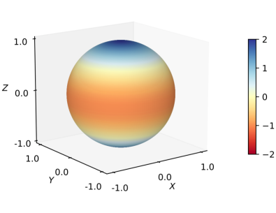
Figure 8: Color-coded surface density plot of $J^{\phi}$ over the two sphere.

We see that in the presence of a constant external magnetic field, the quantum confined particle (to a two dimensional curved surface) experiences both attractive and repulsive dynamical Lorenz force interactions, which will feed back upon the geometrodynamics of the curved surface. To incorporate these new features, the action principle of (10) needs to be augmented in the following form:

$$\begin{split}S=&\frac{\hbar^{2}}{2m}\int d^{2}x\sqrt{h}\\ &e^{-(\varphi^{*}+\varphi)}\left\{D^{*}_{a}\varphi^{*}D^{a}\varphi+\mathcal{R}/2-\mathcal{K}^{2}/4-\epsilon-\frac{1}{4}\Phi F^{2}\right\},\end{split}$$ (27)

where we now consider a complex dilaton, $\Phi=2me^{(\varphi^{*}+\varphi)}/\hbar^{2}$ and $F^{2}=F_{ab}F^{ab}$. This necessary augmentation will alter the resulting geometrodynamical Einstein equation of motion (15), given the $U(1)$ energy momentum tensor in terms of its functional generator:

$$\frac{-2}{\sqrt{h}}\frac{\delta S_{U(1)}}{\delta h^{ab}}\equiv T^{U(1)}_{ab}=-\frac{1}{4}h_{ab}F^{2}+h^{cd}F_{ac}F_{bd},$$ (28)

and adds additional new features to the shape optimization procedures outlined in previous sections. Additionally, the variation of the above total action (27) with respect to the pullback field $A_{a}$ will give rise to an additional equation of motion or constraint, given the functional generator equation for $U(1)$ symmetry:

$$\frac{\delta S}{\delta A_{a}}\equiv J^{a}.$$ (29)

This is in part due to the gauge covariant derivative $D_{a}$ exhibiting $A_{a}$ dependence and where

$$\Phi J_{a}=ie\left(\varphi^{*}\nabla_{a}\varphi-\varphi\nabla_{a}\varphi^{*}\right)+2e^{2}\varphi^{*}A_{a}\varphi$$ (30)

is the previously encountered conserved induced surface Nöther current in terms of the complex dilaton. This new feature, which is also missing in previous research endeavors, will help and allow for more numerical constraints in the shape optimization endeavor. To summarize without loss of generality, let us consider the simplified case for a real dilaton $\varphi^{*}=\varphi$. In this case the total geometrodynamical shape optimization problem reduces to the simultaneous solution of the following equations of motion:

$$\begin{cases}-\frac{\hbar^{2}}{2m}\frac{1}{\sqrt{h}}\partial_{a}\left(\sqrt{h}h^{ab}\partial_{b}\psi_{2D}\right)+\\ -\frac{\hbar^{2}}{2m}\left\{\left(\mathcal{K}/2\right)^{2}-\mathcal{R}/2\right\}\psi_{2D}=E_{2D}\psi_{2D}&\text{{\footnotesize daCSEq}}\\ -\mathcal{K}^{2}/4+\epsilon+2\nabla_{a}\varphi\nabla^{a}\varphi-\square\varphi+\frac{m}{4\hbar^{2}}F^{2}=0&\text{{\footnotesize EEq}}\\ \text{and~{}}\nabla_{b}F^{ab}=-J^{a}&\text{{\footnotesize MEq}}\end{cases},$$ (31)

which are the da Costa Schrödinger equation with induces curvature surface potentials, the Einstein equation and the pulled back induced Maxwell equation. We should note here that despite starting this section with a simplistic example, the above shape optimization equations are not specific to any given example of a quantum confined particle within a given external field configuration, but instead it is a recipe for any general curved two dimensional surface in any arbitrary external field configuration.

V Conclusion

The seminal work and contribution of R. C. T. da Costa cannot be credited enough and overstated in initiating a near revolution before their time. This pioneering work combined the arts of differential geometry and quantum mechanics before the advent of string theory, string theory’s $AdS/CFT$ correspondence, $AdS/CMT$ correspondence and the general gauge gravity correspondence. In fact, the majority of research explosion based upon this paradigm has spawned only in the last decade, as discussed in the introduction.

However, the majority or even entirety of this explosion revolves around carbon copies of solving, numerically or analytical limiting cases of the da Costa Schrödinger equation in (7) only. What we have done in this article is formulate the first novel extension by showing how to implement the da Costa paradigm as a basis for a geometrodynamical shape optimization of the two dimensional curved surfaces with an initial quantum confined eigensystem, a fundamental question and problem in the current semiconductor (device manufacturing) field of researchGentile et al. (2022).

In this work, we have performed an initial proof of concept perturbative calculation of how the two dimensional curved geometry would be deformed given the feedback-work exhibited by the initial confined eigensystem. Additionally, we have laid the basis ground work formulation for how to extend our work within a full numerical iterative solution approach with any given external electromagnetic field configuration. In doing so, we have relied on the finite element analysis method rooted within a stationary action principle.

Some theoretical considerations and comments are due. First, the action in (9) is not a classical one, but should be interpreted as a quantum effective one, since the variation of (9) with respect to the wave function $\psi$ yields the quantum mechanical Schrödinger equation. In other words, (9) is the effective action defend in the canonical way:

$$S=\Gamma_{eff}(\psi)=-i\ln{(Z)},$$ (32)

where

$$Z=\int\mathcal{D}xe^{iS_{cl}(x)}$$ (33)

is the partition function of the classical action, $S_{cl}(x)$. Now, this implies that the Einstein equation in (14) is a quantum mechanical energy momentum tensor:

$$\begin{split}\langle T_{ab}\rangle=&\left\{-\frac{1}{2}h_{ab}\left(\partial_{c}\varphi\partial^{c}\varphi-\frac{\mathcal{K}^{2}}{4}-\epsilon\right)+\partial_{a}\varphi\partial_{b}\varphi+\right.\\ &\left.-\frac{1}{2}\mathcal{K}k_{ab}\right\}e^{-2\varphi}+\frac{1}{2}\left(h_{ab}\square e^{-2\varphi}-\nabla_{a}\nabla_{b}e^{-2\varphi}\right)\end{split},$$ (34)

since

$$\begin{split}\langle T_{ab}\rangle=&\int\mathcal{D}x\left(T_{ab}\right)e^{iS_{cl}(x)}=\int\mathcal{D}x\left(\frac{-2}{\sqrt{h}}\frac{\delta}{\delta h^{ab}}\right)e^{iS_{cl}(x)}\\ =&\frac{-2}{\sqrt{h}}\frac{\delta}{\delta h^{ab}}\int\mathcal{D}xe^{iS_{cl}(x)}=\frac{-2}{\sqrt{h}}\frac{\delta}{\delta h^{ab}}Z\\ =&iZ\frac{-2}{\sqrt{h}}\frac{\delta}{\delta h^{ab}}\Gamma_{eff}(\psi),\end{split}$$ (35)

where we have used the functional generator of $T_{ab}$ and the wave function $\psi$ acts like an auxiliary field for the sake of locality restoration. The above yields the equation of motion in (14) modulo an arbitrary normalization of $iZ$. Additionally, $\langle T_{ab}\rangle$ above is a renormalized energy momentum tensor (EMT), since it satisfies a Bianchi identity. However, what is an important question for the semiconductor and or materials science researchers is, what combination of the above renormalized stress tensor is conserved and or not. In other words, what combination of the above EMT contributes to the two dimensional gravitation anomaly cancelation. Dissecting this detail in (14) would be a first step towards isolating and incorporation materialistic properties of the two dimensional curved surface into the shape optimization procedure. This is a matter for future research and work.