Early Stopping by Correlating Online Indicators in Neural Networks

Abstract

In order to minimize the generalization error in neural networks, a novel technique to identify overfitting phenomena when training the learner is formally introduced. This enables support of a reliable and trustworthy early stopping condition, thus improving the predictive power of that type of modeling. Our proposal exploits the correlation over time in a collection of online indicators, namely characteristic functions for indicating if a set of hypotheses are met, associated with a range of independent stopping conditions built from a canary judgement to evaluate the presence of overfitting. That way, we provide a formal basis for decision making in terms of interrupting the learning process.

As opposed to previous approaches focused on a single criterion, we take advantage of subsidiarities between independent assessments, thus seeking both a wider operating range and greater diagnostic reliability. With a view to illustrating the effectiveness of the halting condition described, we choose to work in the sphere of natural language processing, an operational continuum increasingly based on machine learning. As a case study, we focus on parser generation, one of the most demanding and complex tasks in the domain. The selection of cross-validation as a canary function enables an actual comparison with the most representative early stopping conditions based on overfitting identification, pointing to a promising start toward an optimal bias and variance control.

1 Introduction

A neural network (nn) (Hinton, 1989; Nilsson, 1990; Rumelhart et al., 1986) is a machine learning (ml) system that mimics the behavior of the human brain (McCulloch and Pitts, 1988) for capturing underlying relationships in a set of data from a collection of training examples. Referred to as generalization, this ability to correctly apply the knowledge gained to new situations is a common reference of how accurately a ml algorithm is capable of interacting in practice, and is usually measured by the generalization error. Looking for a suitable representation and better use of data, a nn can integrate multiple layers to progressively extract higher-level features from the raw input. We then talk about deep learning (dl) architectures (Bengio et al., 2013; LeCun et al., 2015; Schmidhuber, 2015), an evolution from the shallow one with profound implications for the expressiveness of the models generated (Bianchini and Scarselli, 2014), but that, in any case, requires generalization errors to be minimized if we want to exploit their potential to the full. At this point, a key factor to consider is the avoidance of overfitting phenomena. Also known as overlearning or overtraining, this concept refers to the production of an analysis by a learner that corresponds too closely to the training set. When that happens, the resulting model may fail to reliably predict future observations.

Overfitting arises in models with low bias and high variance, i.e., when the learner focuses on the detail and/or noise in the training data, often as a result of its structural complexity. That way, in generating large parameter spaces of possibly billions of trainable items (Goodfellow et al., 2016), nns are prone to overfitting behavior (Geman et al., 1992). Since neither bias nor variance are monotonic even in simple cases (Baldi and Chauvin, 1991), it is not always possible to establish when an increase in generalization error signals true overfitting, which explains both the need to simplify the hypotheses for the generated models and to have robust diagnostic strategies. Following Prechelt (1997), we then talk about regularization in the first case and early stopping in the second one.

There are basically two ways of applying regularization: reducing the number of dimensions of the parameter space –usually the connection weights in the network– or reducing the effective size of each dimension. In the latter case, weight decay (Krogh and Hertz, 1992) has become a reference method, while in the first one a number of different approaches have been proposed, including greedy constructive learning (Fahlman and Lebiere, 1990), weight sharing (Nowlan and Hinton, 1992), pruning (Hassibi and Stork, 1993) and noise injection (Holmstrom and Koistinen, 1992). In contrast to this kind of techniques, early stopping (Morgan and Bourlard, 1990) does not aim to directly eliminate overfitting, but rather to stop training when there are reasons to suspect it is occurring. While on paper one might think that this is not the best way to deal with the problem, Bishop (1995) proves that it leads to similar solutions to regularization and, in fact, it can be viewed as regularization over time (Sjöberg and Ljung, 1995). Moreover, its potential as a complement to classic regularization routines and its conceptual simplicity implies lower computational complexity and greater effectiveness (Finnoff et al., 1993; Raskutti et al., 2014), making this a particularly interesting strategy from a practical point of view. This, the design of early stopping conditions, sets the context within which we approach the study of regularization in dl-based learning environments. With that in mind, we first review in Section 2 the methodologies that served as inspiration, as well as our contributions. Next, Section 3 reviews the formal basis supporting the proposal described in full in Section 4. In Section 5, we introduce the testing frame, including both the monitoring structure and a quality metric, for the experiments described and analyzed in Section 6. Finally, Section 7 presents our conclusions.

2 Related work and contribution

Early stopping strategies for nns can be roughly classified according to whether or not a validation set, different from the training set, is considered to monitor learning performance using some kind of quality metric. However, because this latter is mostly based on cross-validation, as is the case for the mean squared error distance, differentiation is often done by the use or non-use of such criteria.

2.1 Early stopping without cross-validation

While the simplest approach is to set the number of epochs used to generate the model, this is not, strictly speaking, a stopping condition because it is unrelated to the level of overfitting in learning. In fact, some authors (Lodwich et al., 2009) prefer the term primary rule, in the sense that the condition is met a fortiori at some point, thus providing a frame to evaluate other secondary rules that cannot be guaranteed to trigger. More formally, Cataltepe et al. (1999) show that, in the absence of information other than the training examples, the generalization error is an increasing function of the training one. Thus, an optimal choice for an early stopping solution should probably be any one associated with the minimum in this latter, although no method has been described to compute it. For their part, Liu et al. (2008) define a signal-to-noise-ratio figure (snrf) to measure the goodness-of-fit using the training error, which enables the detection of overfitting without the use of a separate validation set. However, there are two problems with this criterion (Piotrowski and Napiorkowski, 2013) that make its application problematic. First of all, it depends only on sample size, and so fails to take into account the nature and quality of real-world data. Secondly, it may produce negative values for multidimensional nns, thus resulting in immediate stopping.

Other works address the question from a statistical perspective, seeking a trade-off between nn complexity and training error. For linear systems, Wang et al. (1994) analyze the average optimal stopping time from the probability density error in training data. Unfortunately, this approach is only useful for nns where output weights are being trained and there is no hidden layer training. From a more operational perspective, substantial research focuses on boosting ml, which produces accurate prediction criteria by minimizing a loss function that combines rough and moderately inaccurate rules-of-thumb. For early stopping,  Buhlmann and Yu (2003) prove optimality in the case of fixed design regression, although with a rule that is not computable from the data. More generally, Zhang and Yu (2005) establish universal consistency and convergence upper bounds for convex loss regularizers.

To facilitate practically useful outcomes, subsequent works simplify the hypotheses for overfitting estimators, assuming that, instead of convex or linear combinations of functions, the underlying loss function belong to a reproducing kernel Hilbert space (rkhs). So, Yao et al. (2007) report faster and optimal convergence rates, but do not analyze lower bounds. More recent works overcome this drawback when the upper bounds are improved by studying the eigenvalues of the kernel matrix, thus yielding minimax optimal rates of estimation for a broad class of loss functions and various kernel functions. This is, for example, the case of conjugate gradient (Blanchard and Krämer, 2010), boosting (Raskutti et al., 2014) or gradient descent (Blanchard and Mücke, 2018) algorithms. Unfortunately, such proposals require an unnaturally large –asymptotic– sample size, which not only comes with a considerable computational overhead, but also tends to be suboptimal in practice. Wei et al. (2017), on the other hand, provide similar guarantees without having to calculate all the eigenvalues, although the procedure is unimplementable in practice.

2.2 Early stopping with cross-validation

The idea here is to use the accuracy reached by a model on the validation dataset as an indicator of its generalization error (Morgan and Bourlard, 1990). As the goal is to minimize the error, learning is stopped when deteriorating performance is interpreted as a sign of overfitting. This poses a non-obvious question, as the error in a validation set often has more than one local minimum, so the problem is solvable only when the initial weights of the nn are small enough (Baldi and Chauvin, 1991). Otherwise, and by fixing training collection and initial weights, Dodier (1996) proves that for finite validation sets there is a dispersion of stopping points around the best one, i.e., the most probable with the least generalization error, which increases the expected generalization error. Then, Amari et al. (1997) statistically estimate the optimal split proportion between validation and training data to obtain optimum performance, although the proposal holds asymptotically and is not practical. Such a lack of simple formal solutions to address the halting issue has supported the implementation of a wide variety of naïve strategies, all of which are largely unreliable. Typically they involve stopping the first time a given accuracy value is attained or after a number of iterations is performed without measurable improvement (Shao et al., 2011). It may also be plausible to stop when performance begins to become erratic or the curves that reflect its evolution in training and validation sets begin to cross (Lodwich et al., 2009).

It is within this frame that Prechelt (1997) empirically reports three families of stopping criteria, indexed by a tuning parameter ($\alpha$) to permit small excursions in the validation error: generalization loss ($\mbox{\sc gl}_{\alpha}$), productivity quotient ($\mbox{\sc pq}_{\alpha}$) and uninterrupted progress ($\mbox{\sc up}_{\alpha}$). The first of these criteria stops learning as soon as the relative increase in the validation error exceeds $\alpha$. To avoid stopping when the training error drops rapidly, because this would give the generalization losses a chance to be repaired, the second condition waits until the ratio of gl to training progress in a strip of epochs is greater than $\alpha$. The third criterion, up, suggests stopping when the validation error keeps increasing for $\alpha$ successive strips.

Although Prechelt’s metrics should allow us to make a choice based on efficiency, effectiveness or robustness concerns, no metric seems to predominate in terms of average generalization performance. So, while longer training time appears to improve generalization performance in all cases, the pq proves to be most cost-effective only for sufficiently small nns. Either way, Prechelt’s proposal has inspired a good part of further work in practical early stopping in dl, and also in evolutionary algorithms, typically through genetic programming (gp) techniques in which the counterpart of the loss function is identified with the fitness function. Specifically, Foreman and Evett (2005) study the use of online indicators from the Prechelt’s metrics with cross-validation as canary function, and as also done in a later work by Vanneschi et al. (2010), they raise the interest of exploring the correlation between fitness in the training set and the validation one. Alas, to the latter possibility, (Vanneschi et al., 2010) merely apply the concept from a visual point of view, with no formal basis. Turning to Foreman and Evett (2005), they limit themselves to a brief discussion without including technical details, which concludes by proposing the combination of a correlation coefficient –which they do not even identify– as the primary condition and pq as the complementary one. Tuite et al. (2011), however, disagree with this approach and report the pq to be less effective in gp, a behavior that Nguyen et al. (2012) associate with the use of excessively small values for the $\alpha$ tuning parameter. This lack of consensus is also reflected in the nn sphere, where Piotrowski and Napiorkowski (2013) adopt the simplest gl and terminate training when the validation error exceeds its previously noted minimum by 20%. More recently, Wang and Yan (2017) have extended Prechelt’s approach by combining the probability density function error of the unlabeled sample data and the validation error of the labeled ones, although the impact on the reduction of the generalization error seems limited.

A different view of the issue is to seek to improve efficiency by selecting the validation series on the basis of its mean dynamic correlation with forecast performances, in the complete training data (Michalak and Raciborski, 2005). However, the validation set needs to be sufficiently large, even when the observed enhancement is statistically significant. Nonetheless, those authors implicitly suggest the grouping of single conditions to generate a compound rule that stops when one of those so determines, an approach later explored by Lodwich et al. (2009) for six families of single criteria, including Prechelt’s ones. Their tests confirm the apparent superiority of pq over the rest of the individual rules, while the top results seem to require criteria to be coupled, with ensembles based on $\mbox{\sc pq}_{3}$ performing best.

2.3 Our contribution

Against this backdrop, we formally describe and test an early stopping procedure –which we have called coi, for correlation of online indicators– with a view to reducing the risk of a misguided early stopping, but also to improving the trade-off between training effort and generalization error. In order to provide the adaptability to each learning process that this requires, our proposal exploits the properties of potentially complementary halting rules, with the sole condition that the latter are organized as a repository of indicators for some canary function regarding overfitting phenomena. The technique takes a correlation coefficient as a measure of the degree of agreement in the diagnosis by the individual rules, which are assumed to be defined by sets of variables that are mutually independent. This allows us to put ourselves in a context in which the principle of the common cause holds, thus supporting the correctness of a stopping criterion based on sufficiently broad agreement between at least two of the diagnoses. Thus, once the user has set a correlation coefficient and a confidence threshold for it, the halting decision is made over time according to the highest alignment between a pair of individual indicators.

We choose the natural language processing (nlp), a set of computational methods aimed at processing and understanding human languages, as test environment. This domain, increasingly linked to data-driven models (Jones, 1994), is featured by a growing interest in using dl techniques (Goldberg and Hirst, 2017; Young et al., 2018). The main reason is the ability to automatically generate multilevel features to produce distributed representations from texts at both word (Mikolov et al., 2010) and syntactic (Collobert et al., 2011) levels. Also known as embeddings, these features can be used as a first processing layer in dl-based nlp models. This brings a revolution because, apart from minimizing the need for time-intensive engineering work and hand-designed resources, the latter are often incomplete or sparse. It is therefore expected that advances in computational power and parallelization (Coates et al., 2013; Raina et al., 2009), together with the availability of large training datasets, offer a bright future for these methods, which justifies our choice.

3 Formal framework

Below we review the fundamentals of the abstract model that will be introduced later, namely the use of online indicators for canary functions as an early warning mechanism for assessing the risk of overfitting in nns, and the definition of a trusted decision-making scenario from the correlation of different criteria.

3.1 Canary functions and online indicators for overfitting identification

To recognize when overfitting may be starting to occur, precise characterization is required to capture the operational meaning behind this idea. A close reference is the notion of canary function, introduced to solve the issue in gp (Evett et al., 1998). Such functions differ from the fitness ones in that their value begins to degrade at about the same time overfitting starts. Following this path, Foreman and Evett (2005) take advantage of cross-validation approaches, using performance divergence between training and validation sets to determine when overfitting occurs. Unfortunately, a problem arises with practical implementations, since it is difficult to estimate the actual scale of such deviation from the local perspective of an iterative learning scheme. Drawing inspiration from the stopping conditions described by Prechelt (1997) for nns, the authors use Boolean functions –called online indicators– to evaluate from data available at each generation of a gp run whether that disparity is significant. In addition, they hypothesize that the correlation coefficient between the fitness of the best individual of the generation with respect to the training set, and the fitness of the best individual of the generation with respect to the validation one at the end of each generation should also be a strong divergence signal.

Following this path, we adapt the concept of a canary function to nns by using a loss function instead of a fitness one, as that permits us to reflect performance discrepancy between the training and validation sets. The notion of online indicator is then readjusted accordingly, allowing Prechelt’s stopping criteria to be applied to the task, as well as any correlation coefficient for training and validation set performance.

3.2 An explanatory basis for correlating criteria

The core of our work rests on the idea that the stopping decisions for several indicators using the same canary function can yield complementary insights and thus increasing the reliability of individual criteria, i.e. predictive power can be enhanced through an appropriate combination of such criteria. It is therefore necessary to determine the conditions under which a solution of this type is applicable. This means, first and foremost, establishing a theoretical framework for their analysis, on which to then define a well-founded reasoning scheme to ensure the correctness of our approach.

3.2.1 The principle of the common cause

In essence, our initial argument relies on a metaphysical claim that refers to similar state-of-the-art interpretations in the philosophy of causation (Mill, 1868; Russell, 1948), stating that:

“if an improbable coincidence has occurred, there must exist a common cause”

However, since this says nothing about how to characterize cause/effect relationships, it is not helpful for implementation purposes, although it does give our proposal meaning. Reichenbach (1956) fills this gap by a methodological claim based on a probabilistic criterion. Suppose events $A$ and $B$ are positively correlated, namely

$$p(A\;\&\;B)>p(A)\;p(B)$$ (1)

and assume that neither $A$ nor $B$ is a cause of the other. Then Reichenbach maintains that there is a common cause $C$, of $A$ and $B$, meeting the conditions:

$$p(A\;\&\;B\mid C)=p(A\mid C)\;p(B\mid C)$$ (2)

$$p(A\;\&\;B\mid\neg C)=p(A\mid\neg C)\;p(B\mid\neg C)$$ (3)

$$p(A\mid C)>p(A\mid\neg C)$$ (4)

$$p(B\mid C)>p(B\mid\neg C)$$ (5)

In particular, Eq. 2 (resp. Eq. 3) is construed to mean that $C$ (resp. $\neg C$) screens off the correlation between $A$ and $B$. This correlation disappears when we take into account the common cause, which is to say that $A$ and $B$ are then probabilistically independent. Meanwhile, Eq. 4 (resp. Eq. 5) states that $C$ is a cause for $A$ (resp. $B$). Altogether, Eqs. 2-5 characterize what is defined as a conjunctive fork $ACB$, namely a causal structure $A\leftarrow C\rightarrow B$.

According to the state-of-the-art (Reichenbach, 1956; San Pedro and Suárez, 2009), we will refer to the metaphysical claim as the postulate of the common cause (poscc), to the methodological claim as the criterion for common causes (critcc) and to the conjunction of both claims as the principle of the common cause (pcc). This provides us with a theoretical framework for causation analysis by introducing probabilistic causality, a notion in philosophy whose main message is that causes change the probabilities of their effects (Cartwright, 1979; Eells, 1991; Skyrms, 1981; Suppes, 1970).

3.2.2 The explanatory power of different causal assumptions

Unfortunately, although Reichenbach’s view confers the predictibility necessary to give support to our proposal, the pcc cannot be accepted at face value because the critcc may fail. This may occur particularly when the correlated events are logically related or spatio-temporally overlapping (Hitchcock, 2012), and also when there is an attempt to apply it in domains where classic causal intuition is no longer valid. The latter scenario is typically the case of quantum mechanics, whose recent success has renewed interest in probabilistic causation to the detriment of deterministic approaches (Hume, 1904) –also called regular approaches– according to which causes are invariably followed by their effects.

It thus becomes evident that critcc is not a sufficient condition for a conjunctive fork, which justifies the formulation of theories close to pcc but requiring that the likely cause occurs at an earlier time than the correlated effects (Arntzenius, 1993; Van Fraassen, 1982). Alternatively, Hofer-Szabó et al. (1998, 2013) seek a screening-off common cause, as described by Reichenbach, by extending the original probability space to another causally closed space, while the question remains whether the common causes thus detected represent anything physically real. Finally, other authors (Cartwright, 1988; Salmon, 1984) simply accept the validity of pcc, but only under a revision of critcc. In short, there is no agreement regarding the status of pcc and its relationship to the notion of common cause (Hofer-Szabó et al., 2013; Forster, 2014).

Thankfully, in deterministic contexts with mutually independent events caused by an earlier one, the pcc holds even when the operational conditions do not allow for trivialization. It can therefore be interpreted to reflect the imperfect knowledge of the causal system, thus justifying its application (Arntzenius, 2010).

4 Abstract model

The theoretical foundations of our proposal are explained below for later interpretation from an operational point of view. We first explain the working hypotheses and notational support, and then formally describe our abstract model to finally establish its correctness.

4.1 Working hypotheses and notational support

Let $\mathbb{R}$ be the real number line and $\mathbb{N}$ the natural number line, with $0\not\in\mathbb{N}$. We are given a fixed sampling database ${\mathcal{D}}={\mathcal{D}}_{\textit{tr}}\cup{\mathcal{D}}_{\textit{va}}\cup{\mathcal{D}}_{\textit{te}}$, referring respectively to test, training and validation sets. Each ${\mathcal{D}}_{j}:=\{(x^{i}_{j},f^{i}_{j})\}_{i=1}^{N_{j}}$ includes inputs $x^{i}_{j}\in\mathbb{R}^{L}$, outputs $f^{i}_{j}\in\mathbb{R}^{M}$ and $L,M,N_{j}\in\mathbb{N}$, with $j\in\{\textit{tr},{\textit{va}},{\textit{te}}\}$. The outputs are assumed to be generated from the inputs in a deterministic causal system according to some unknown distribution $f$ and, hence, $f^{i}_{j}=f(x^{i}_{j}),\forall i\in[1,N_{j}]$. Depending on the ml strategy used, ${\mathcal{D}_{\textit{te}}}$ may or may not be empty.

A dl-based learning scheme, hereafter a kernel, is denoted by ${\mathcal{K}}={\mathcal{N}}^{\pi}[{\mathcal{D}}]$, with ${\mathcal{N}}$ a nn, ${\mathcal{D}}={\mathcal{D}}_{\textit{tr}}\cup{\mathcal{D}}_{\textit{va}}\cup{\mathcal{D}}_{\textit{te}}$ a sampling database and $\pi$ a collection of parameters that includes a propagation function, which can add a bias term to its result but also possibly an activation function. We then use ${\mathcal{K}}[e]$ to refer to the model generated at epoch $e$ from such a learning scheme, and $E_{j}^{\mathcal{K}}[e]$ to refer to the value for it of a loss function –also referred to as an error function– $E$ in ${\mathcal{D}}_{j}\subseteq{\mathcal{D}},j\in\{\textit{tr},{\textit{va}},{\textit{te}}\}$.

Having set $\Upsilon_{c}:=\{c_{i}\}_{i\in I}$ a finite family of online indicators on a canary function $c$ and ${\mathcal{K}}={\mathcal{N}}^{\pi}[{\mathcal{D}}]$ a kernel, we then refer to the value of $c_{i}\in\Upsilon_{c}$ at epoch $e$ as $c_{i}^{\mathcal{K}}[e]$, and the epoch at which $c_{i}$ verifies and the training of ${\mathcal{K}}$ stops as $s_{c_{i}}^{\mathcal{K}}$. The model generated at this latter is labelled as a run ${\mathcal{R}}={\mathcal{N}}^{\pi}_{c_{i}}[{\mathcal{D}}]$, namely ${\mathcal{R}}:={\mathcal{K}}[s_{c_{i}}^{\mathcal{K}}]$. More intuitively, a run is the result of a specific learning process from a kernel ${\mathcal{K}}$, the completion of which is determined by an online indicator $c_{i}$ defined on a given canary function $c$. We can then naturally introduce $E_{j}^{\mathcal{R}}$ as $E_{j}^{\mathcal{K}}[s_{c_{i}}^{\mathcal{K}}]$, i.e. the value of the error function measured for the model associated with the run ${\mathcal{R}}$ when it applies on a database ${\mathcal{D}}_{j}\subseteq{\mathcal{D}},j\in\{\textit{tr},{\textit{va}},{\textit{te}}\}$.

Within the context described above, the precision of an indicator $c_{i}\in\Upsilon_{c}$ in relation to the training procedure represented by the kernel ${\mathcal{K}}$ will be all the greater the closer the epoch at which its termination occurs ($s_{c_{i}}^{\mathcal{K}}$) to the one that determines the time at which the overfitting actually arises, the latter denoted by $\mbox{\em\oe}^{\mathcal{K}}$. For testing purposes, the exact location of the epoch $\mbox{\em\oe}^{\mathcal{K}}$ can be estimated from a sufficiently large number of epochs in ${\mathcal{K}}$, referred to as its horizon, by selecting the iteration that is associated with the lowest validation error.

4.2 Our proposal

Given a kernel ${\mathcal{K}}={\mathcal{N}}^{\pi}[{\mathcal{D}}]$, namely a learning process on a sampling database ${\mathcal{D}}$ using a learner ${\mathcal{N}}$ according to a setting $\pi$, we seek to identify the epoch $\mbox{\em\oe}^{\mathcal{K}}$ in which training should stop to prevent overfitting. Taking the values provided by a canary function $c$ as basis for decision making on the diagnosis of this type of phenomena, and $\Upsilon_{c}:=\{c_{i}\}_{i\in I}$ as a finite set of associated and pairwise independent online indicators defined on it, the idea is to provide robustness for early stopping by exploiting their consensus. To this end, we resort to a correlation coefficient $\aleph$, which we assume to be compatible with the underlying distribution of the values generated by such indicators.

Thus, training stops when at least two such indicators so advise within a training strip of length $k$, i.e., a sequence of $k$ epochs numbered $n+1\cdots n+k$ where $n$ is divisible by $k$, in which their $\aleph$-correlation is above a threshold. In particular, the indicators do not need to agree on the same epochs, thereby introducing a limited level of asynchronicity in order to make the condition more flexible. Against this backdrop, we first capture that notion of flexible $\aleph$-correlation within a training strip of length $k$ at epoch $e$ by:

$$c_{\textit{coi}[\aleph,k]}^{\mathcal{K}}[e]:=\max_{\iota,\jmath\in I}\{0,\;\aleph_{{\mathcal{C}}_{\iota}^{\mathcal{K}}[k,e]}^{{\mathcal{C}}_{\jmath}^{\mathcal{K}}[k,e]}\;\mbox{\em such that}\;\exists\;i,j\in[k-1,0]\;\mbox{\em for which}\;c_{\imath}^{\mathcal{K}}[e-i]\;\mbox{\em and}\;c_{\jmath}^{\mathcal{K}}[e-j]\}$$ (6)

with ${\mathcal{C}}_{\imath}^{\mathcal{K}}[k,e]:=\{c_{\imath}^{\mathcal{K}}[e-k+1],\dots,c_{\imath}^{\mathcal{K}}[e]\},\;\forall\imath\in I$. Having fixed a minimum value $\alpha_{\aleph}$, the corresponding online indicator is then given by the Boolean expression:

$$c_{\textit{coi}[\aleph,k,\alpha_{\aleph}]}^{\mathcal{K}}[e]:=[c_{\textit{coi}[\aleph,k]}^{\mathcal{K}}[e]>\alpha_{\aleph}]$$ (7)

which is true when the value $c_{\textit{coi}[\aleph,k]}^{\mathcal{K}}[e]$ calculated from Eq. 6 is greater than $\alpha_{\aleph}$, and false otherwise.

4.3 Correctness

Once our working hypotheses have been established, the goal is to prove that the positive correlation between online indicators increases the reliability of the diagnosis of overfitting phenomena. Firstly, this implies verifying the conditions of applicability for the critcc –the methodological claim of the pcc–, which will allow us to conclude that there is a common cause behind such a statistical relationship and that this is not the result of a dependency link between the indicators. Afterwards, it will be sufficient to identify that such common cause is the degradation of values provided by the canary function considered, which we assume to be at the origin of a generalization loss and, therefore, also of a potential overfitting of the ml process.

4.3.1 Applicability for the critcc

We are talking in this case about an immediate conclusion because our causal structure is supposedly regular and the observed variables, namely the online indicators, are also assumed to be free from causal relationships between them. In other words, our working hypotheses ensure that the critcc is interpretable as a necessary and sufficient condition on common causes (Arntzenius, 2010; San Pedro and Suárez, 2009).

4.3.2 Identification of the common cause

In the previously set correctness context, the only remaining task is to identify the common cause behind any positive correlation as the increase in the canary function of the performance discrepancy between the training sets and the validation ones. We are again talking about an immediate conclusion, this time derived from the very notion of an online indicator, which is essentially a Boolean that determines whether performance reduction is significant enough to suspect that overfitting occurs. In other words, the common cause is the observed decline in learning acquisition.

The pcc thus provides, by means of a simple probabilistic approach to causation, a way of enhancing reliability in the diagnosis of overfitting phenomena independent of temporary variations in the error function over the course of an ml process. Put another way, decision making based on the correlation of complementary stopping criteria diminishes the risk of wrong appraisal, often resulting from simple local irregularities in the values generated by the canary functions.

5 Testing frame

To support our conclusions, we design a categorizing protocol for early stopping criteria based on a quality metric. In order to guarantee its reliability, the conditions under which the experiments take place are normalized by introducing a specific monitoring architecture for data collection.

5.1 Monitoring structure

With the purpose of enabling the monitoring of the trials in our testing frame, it is first necessary to design a structure that allows the online indicators to compete on fair terms. This implies organizing our study around a family of local testing frames that encapsulate those common assessment conditions according to different combinations of learners and sampling databases, i.e. different kernels. Against this backdrop, our evaluation basis is the previously entered run structure ${\mathcal{N}}_{c_{i}}^{\pi}[{\mathcal{D}}]$, essentially a model generated from a kernel ${\mathcal{N}}^{\pi}[{\mathcal{D}}]$, namely a training task on a sampling database ${\mathcal{D}}$ according to a given learning architecture ${\mathcal{N}}$ for a particular setting $\pi$, and a stopping criterion fixed by an online indicator $c_{i}$ within a collection $\Upsilon_{c}$ in which all have been defined on the same canary function $c$.

Obviously, we also need to set a reference base for our research findings which should be shared by the set of local evaluation settings considered in order to provide a comprehensible general overview of our proposal. We then assume $c_{\wp[h]}$ to be an optimal online indicator for a canary function $c$, with values provided by an omniscient oracle on a horizon $h$ in such a way that, whatever the run ${\mathcal{N}}_{c_{\wp[h]}}^{\pi}[{\mathcal{D}}]$ considered, $\mbox{\em\oe}^{\mathcal{K}}=s_{c_{\wp[h]}}^{\mathcal{K}}$ for its corresponding kernel ${\mathcal{K}}={\mathcal{N}}^{\pi}[{\mathcal{D}}]$. In other words, the epoch $\mbox{\em\oe}^{\mathcal{K}}$ in which the overfitting occurs, is the same epoch $s_{c_{\wp[h]}}^{\mathcal{K}}$ at which the online indicator $c_{\wp[h]}$ indicates it, thereby justifying its referential character.

Once a family $I$ of kernels is fixed, the study of a learning scheme $i\in I$ is formalized around the notion of local testing frame $\mathcal{L}_{i}^{\Upsilon_{c}}:=\{{\mathcal{N}}^{\pi}_{c_{\iota}}[{\mathcal{D}}],\;c_{\iota}\in\Upsilon_{c}\cup\{c_{\wp[h]}\}\}$. We are then talking about a set of runs defined on the same kernel ${\mathcal{N}}^{\pi}[{\mathcal{D}}]$ and only distinguishable by their online indicator $c_{\iota}$ taken from a finite set $\Upsilon_{c}$ related to a canary function $c$, which also includes ${\mathcal{N}}_{c_{\wp[h]}}^{\pi}[{\mathcal{D}}]$ as baseline. That way, the collection ${\mathcal{L}}:=\{\mathcal{L}_{i}^{\Upsilon_{c}}\}_{i\in I}$ of local testing frames becomes naturally our monitoring structure.

5.2 Performance metric

According to the principle of maximum expected utility (meu) (Meek et al., 2002), we interpret the performance associated with a run as the search for a satisfactory cost/benefit trade-off, involving both quantitative and qualitative considerations. For the quantitative considerations, we take into account the final computational cost, which depends on the degree of control exercised by the user over the ml process. In its absence, as in our case, those costs are the sum of the data acquisition, error and model induction costs (Weiss and Tian, 2008). Since the kernel ${\mathcal{N}}^{\pi}[{\mathcal{D}}]$ is common to all runs in a local testing frame $\mathcal{L}^{\Upsilon_{c}}:=\{{\mathcal{N}}^{\pi}_{c_{\iota}}[{\mathcal{D}}],\;c_{\iota}\in\Upsilon_{c}\cup\{c_{\wp[h]}\}\}$, so too are their acquisition costs, while error (resp. model induction) costs are proportional to the cumulative error for each run in the validation dataset (resp. the number of epochs applied). As for the qualitative considerations, baseline runs provide an easy to understand gold standard within local testing frames, thereby offering a simple and practical framework to assess online indicators.

Definition 1.

Let ${\mathcal{L}}^{\Upsilon_{c}}:=\{{\mathcal{N}}^{\pi}_{c_{\iota}}[{\mathcal{D}}],\;c_{\iota}\in\Upsilon_{c}\cup\{c_{\wp[h]}\}\}$ be a local testing frame on a kernel ${\mathcal{K}}={\mathcal{N}}^{\pi}[{\mathcal{D}}]$, with baseline ${\mathcal{B}}$. We define the normalized meu signed deviation (nemesid) of a run ${\mathcal{R}}:={\mathcal{N}}^{\pi}_{c_{\iota}}[{\mathcal{D}}]\in{\mathcal{L}}^{\Upsilon_{c}}$ as:

$$\Phi^{\omega_{mi}}_{\omega_{\textit{ea}}}({\mathcal{R}},{\mathcal{L}}^{\Upsilon_{c}}):=\left\{\begin{array}[]{ll}\frac{\mbox{\sc c}^{\omega_{\textit{mi}}}_{\omega_{\textit{ea}}}({\mathcal{R}})-\mbox{\sc c}^{\omega_{\textit{mi}}}_{\omega_{\textit{ea}}}({\mathcal{B}})+\mbox{\sc mcdb}^{\omega_{\textit{mi}}}_{\omega_{\textit{ea}}}({\mathcal{L}}^{\Upsilon_{c}})}{\mbox{\sc mcdb}^{\omega_{mi}}_{\omega_{\textit{ea}}}({\mathcal{L}}^{\Upsilon_{c}})}-1&\mbox{if }\mbox{\sc mcdb}^{\omega_{\textit{mi}}}_{\omega_{\textit{ea}}}({\mathcal{L}}^{\Upsilon_{c}})\neq 0\\ 0&\mbox{otherwise}\end{array}\right.$$ (8)

where

$$\mbox{\sc mcdb}^{\omega_{\textit{mi}}}_{\omega_{\textit{ea}}}({\mathcal{L}}^{\Upsilon_{c}}):=\max_{{\mathcal{R}}\in{\mathcal{L}}^{\Upsilon_{c}}}\mid\mbox{\sc c}^{\omega_{\textit{mi}}}_{\omega_{\textit{ea}}}({\mathcal{R}})-\mbox{\sc c}^{\omega_{\textit{mi}}}_{\omega_{\textit{ea}}}({\mathcal{B}})\mid$$ (9)

captures the maximum cost deviation from the baseline in ${\mathcal{L}}^{\Upsilon_{c}}$ and

$$\mbox{\sc c}^{\omega_{\textit{mi}}}_{\omega_{\textit{ea}}}({\mathcal{R}}):=\omega_{\textit{mi}}\ast s_{c_{\iota}}^{\mathcal{K}}+\omega_{\textit{ea}}\ast E^{\mathcal{R}}_{\textit{va}},\mbox{ such that }\omega_{\textit{mi}},\omega_{\textit{ea}}\in(0,1]$$ (10)

is the cost of ${\mathcal{R}}\in{\mathcal{L}}^{\Upsilon_{c}}$, expressed as the sum of the model induction and error acquisition costs, with processing weights for each epoch and error assumed to be $\omega_{\textit{mi}}$ and $\omega_{\textit{ea}}$, respectively.

As the name implies, nemesid quantifies and normalizes the signed deviation of a run from its baseline in meu terms. Since such baselines are always built on the online indicator supported by the omniscient oracle, this gives us an effective means of estimating the performance of any other indicator through different local testing frames, something that an absolute measure cannot do.

More formally, and once a local testing frame is fixed, nemesid is strictly increasing with respect to the cost of the runs. Since the minimum (resp. maximum) is reached in runs with the lowest (resp. highest) cost compared with the baseline, the codomain is the interval $[-1,1]$. In contrast, the modulus of this metric is strictly decreasing with respect to the utility of the runs, and because the value is null for the baseline, the codomain is now the interval $[0,1]$. Accordingly, the lower its real and absolute nemesid values, the better a run performs. In other words, the most efficient online indicators are those providing rates as close to zero as possible, preferably negative.

6 Experimental results

Given a kernel ${\mathcal{N}}^{\pi}[{\mathcal{D}}]$ representing an ml process over a series of epochs, and taking cross-validation as the canary function $c$, the goal is to illustrate how well our online indicator performs in detecting overfitting.

6.1 Case study

We focus on parser generation in the domain of nlp, not only because of the complexity of annotation in building training data and then learning to capture the relationships at training time, but also because parsers serve as input for other nlp functionalities (Jurafsky and Martin, 2009). From a marked-up text provided by a part-of-speech (pos) tagger, a parser identifies which words modify others and how, resulting in a sentence structure. The rise of dl technologies has propelled the interest in dependency-based methods (Tesnière, 1959). In contrast to classic constituency parses, which hierarchically break text into terminals –words– and non-terminals –syntagms–, dependency parses look at the relationships between pairs of words to produce trees of terminal nodes. The resulting dependency arcs hold between a head, which determines the behavior of the pair, and a dependent, which acts as its modifier or complement (Kubler et al., 2009). These arcs are labeled to supply additional environmental features and are projected to embeddings, that can be more efficiently exploited by semantic-based nlp applications through nns than using other type of techniques (Collobert et al., 2011). All of this fully justifies the appropriateness of our case study.

6.2 Required resources

The objective is to select a set of linguistic and software resources that guarantee a reliable and trustworthy experimental evaluation, taking into account that our operational context is the generation of dl-based dependency parsers. To this end, we focus our attention on the most representative corpora and parser generators in the nlp community.

6.2.1 Linguistic resources

In accordance with the representativeness requirement we have just outlined, these are built from the collection of tree-banks provided by Universal Dependencies (ud) (de Marneffe et al., 2014), an international cooperative project that provides consistent annotation of grammar, including syntactic dependencies and also pos and morphological features, and is freely available online (https://universaldependencies.org/).

The ud treebanks are a collection of parsing datasets manually annotated using a revised version of the conll-x format (Buchholz and Marsi, 2006) called conll-u (https://universaldependencies.org/format.html) and usually partitioned into training, validation and test sets. Taken as a whole, they are a comprehensive repository for numerous human languages, which allows our experimental scope to be broadened beyond the usual resource-rich languages –Chinese (zh), English (en), Farsi (fa), French (fr), German (de), Hindi (hi), Japanese (ja), Polish (pl), Portuguese (pt), Russian (ru) and Spanish (es)– to also include resource-poor languages –Catalan (ca), Basque (eu), Galician (gl) and Serbian (sr). This also ensures that the corpora selected are representative of a wide variety of language families and subfamilies with very different characteristics, including Indo-European (Germanic, Romance and Slavic), Japonic and Sino-Tibetan, as well as a language isolate (eu). Moreover, each language dataset covers different knowledge domains (e.g. legal, news, poetry, wiki, etc), in which case the corresponding training, validation and test sets are aggregated into one set. Whenever possible, erroneous entries are discarded and non-standard data are cleaned. All of this contributes to the aim of defining a reliable testing space for ml.

Tables 1 and 2 summarize details of the databases for resource-rich and resource-poor languages, respectively, differentiating between partitions; italic characters indicate when a validation set is not available and the test set is used instead. Details include the average number of sentences, tokens per sentence and percentages of unknown tokens and unique tokens.

			de	en	es	fr	pl	pt	ru
training	sentences		166,849	21,253	28,492	18,640	31,496	17,992	54,099
	unique tokens	(%)	6.49	7.89	7.92	10.30	17.74	9.55	12.69
	sentence size		18.08	17.65	29.03	23.85	12.27	25.71	17.81
validating	sentences		19,233	3,974	3,054	2,902	3,960	1,770	8,108
	unique tokens	(%)	13.35	16.59	18.56	20.40	32.73	22.65	24.86
	sentence size		17.26	15.76	29.30	19.87	12.07	24.28	17.30
	unknown tokens	(%)	5.46	7.51	5.35	6.41	13.12	5.64	11.69

Table 1: Characteristics of datasets for resource-rich languages

			ca	eu	fa	gl	hi	ja	sr	zh
training	sentences		13,123	5,396	4,798	2,872	13,304	7,125	3,328	3,997
	unique tokens	(%)	7.40	26.34	10.94	15.18	6.01	14.20	22.29	17.78
	sentence size		31.82	13.52	25.23	33.00	21.13	22.48	22.31	24.67
validating	sentences		1,709	1,798	599	1,260	1,659	511	536	500
	unique tokens	(%)	16.40	36.53	24.50	20.85	15.16	31.76	37.40	34.00
	sentence size		33.05	13.40	26.43	31.65	21.23	22.46	22.38	25.33
	unknown tokens	(%)	5.78	19.14	10.46	11.05	5.51	6.23	18.58	13.03

Table 2: Characteristics of datasets for resource-poor languages

6.2.2 Software resources

Analogously to the case of the linguistic resources, we use the most popular and efficient generators for dl-based dependency parsers from the neuronlp2 project (Ma and Hovy, 2016). It includes implementations for state-of-the-art models for a wide range of core tasks, including parsing (Liu et al., 2019; Ma et al., 2018; Rotman and Reichart, 2019), pos tagging (Tourille et al., 2018) and named entity recognition (Magnini et al., 2020), all publicly available online (https://github.com/XuezheMax/NeuroNLP2). Focusing on parsing, the scope of our case study, we chose to work with two particular encoders:

• Deep biaffine attention (biaf) (Dozat and Manning, 2017).

• Maximum spanning tree (neuromst) (Ma and Hovy, 2017).

This allows, respectively, coverage of projective and non-projective capabilities  when dealing with dependency-based parsing, precisely the parsing paradigm propelled by the rise of dl technologies.

Both encoders share a basic architecture, structured as a recurrent network using bidirectional long-short term memory (bilstm) (Ma and Hovy, 2016) to encode inputs. Both also operate at word level, although neuromst takes the form of a convolutional neural network (cnn) (LeCun and Bengio, 1998) to exploit information at the character level. As the main distinctive characteristics of each encoder, neuromst-based parsers rely on a conditional log-linear model on top of the neural network to classify dependency labels, while biaf-based ones do this classification via a modified version of bilinear attention (Kim et al., 2018). Unlike neuromst, biaf uses different vectors for different dependency labels to represent each word, thus performing slightly better in exchange for a greater memory requirement. The hyperparameter configuration is similar for both encoders: word embeddings of 300 –obtained from https://fasttext.cc/docs/en/crawl-vectors.html)– dimensions, 3 recurrent layers of 512 neurons, elu activation units, and a uniform dropout of 0.3.

6.3 Testing space

To illustrate how our proposal performs, we need to compare it to other cross-validation-based online indicators. We also need to ensure an appropriate setting of parameters so as to introduce the set of local testing frames that define the testing space.

6.3.1 State-of-the-art online indicators

On the basis of the state-of-the-art in both nns and gp, we describe the online indicators listed below, as referred to a given kernel ${\mathcal{K}}={\mathcal{N}}^{\pi}[{\mathcal{D}}]$. In addition to the primary rule $c_{\textit{mne}[m]}^{\mathcal{K}}$, which fixes the maximum number $m$ of epochs to be executed, the online indicators and also our proposal, $c_{\textit{coi}[\aleph,k,\alpha_{\aleph}]}^{\mathcal{K}}$, are monitored against the baseline $c_{\wp[h]}^{\mathcal{K}}$ provided by an omniscient oracle in a horizon of $h=10^{3}$ epochs.

Generalization loss $(c_{\textit{gl}})$

Training stops when the generalization loss rises above a specific threshold (Prechelt, 1997) relative to the optimal error $E_{\textit{op}}[e]$, i.e., the minimal error observed in epochs up to the current one $e$:

$$E_{\textit{op}}^{\mathcal{K}}[e]:=\min_{\hat{e}\leq e}E_{\textit{va}}^{\mathcal{K}}[\hat{e}]$$ (11)

We then define (as a percentage) the loss at epoch $e$ by:

$$c_{{\textit{gl}}}^{\mathcal{K}}[e]:=100\ast\left(\frac{E_{\textit{va}}^{\mathcal{K}}[e]}{E_{\textit{op}}^{\mathcal{K}}[e]}-1\right)$$ (12)

and, having fixed a maximum value $\alpha$, the corresponding online indicator is given by:

$$c_{{\textit{gl}[\alpha]}}^{\mathcal{K}}[e]:=[c_{{\textit{gl}}}^{\mathcal{K}}[e]>\alpha]$$ (13)

Progress $(c_{\textit{p}[k]})$

Training stops when during a training strip of length $k$, improvements in training error stall below a specific threshold. Progress is measured as the ratio between the average training error during the strip and the minimum one. We then define the progress (in parts per thousand) at epoch $e$ by:

$$c_{\textit{p}[k]}^{\mathcal{K}}[e]:=100\ast\left(\frac{\sum_{\hat{e}=e-k+1}^{e}E_{\textit{tr}}^{\mathcal{K}}[\hat{e}]}{k\ast\min_{\hat{e}=e-k+1}^{e}E_{\textit{tr}}^{\mathcal{K}}[\hat{e}]}-1\right)$$ (14)

Having fixed a minimum value $\alpha$, the corresponding online indicator is given by:

$$c_{{\textit{p}[k,\alpha]}}^{\mathcal{K}}[e]:=[c_{\textit{p}[k]}^{\mathcal{K}}[e]<\alpha]$$ (15)

Comparing with $c_{\textit{gl}}$, $c_{{\textit{p}[k]}}$ is high for unstable phases of training, where the training error goes up instead of down. This was described by Prechelt (1997) and first evaluated by Lodwich et al. (2009) as low progress.

Productivity quotient $(c_{\textit{pq}[k]})$

Training stops when, during a strip of length $k$, there is little chance that the generalization loss can be repaired, which may happen when progress is very rapid. Evaluation is based on a threshold in the ratio to training progress (Prechelt, 1997). We then define the productivity quotient at epoch $e$ as:

$$c_{\textit{pq}[k]}^{\mathcal{K}}[e]:=\frac{c_{\textit{gl}}^{\mathcal{K}}[e]}{c_{\textit{p}[k]}^{\mathcal{K}}[e]}$$ (16)

Having fixed a maximum value $\alpha$, the corresponding online indicator is given by:

$$c_{{\textit{pq}[k,\alpha]}}^{\mathcal{K}}[e]:=[c_{\textit{pq}[k]}^{\mathcal{K}}[e]>\alpha]$$ (17)

Comparing with $c_{\textit{gl}}$, $c_{{\textit{pq}[k]}}$ does not report overfitting until the training error begins to decrease slowly, which is of interest if we can assume a higher generalization loss given a greater progress on the training set.

Uninterrupted progress $(c_{\textit{up}[s,k]})$

Training stops when, during a sequence of $s$ strips of length $k$, the generalization error increases (Prechelt, 1997). We then assume that overfitting has begun independently of the size of the increases. Thus, we recursively define uninterrupted progress at epoch $e$ as:

$$c_{\textit{up}[s,k]}^{\mathcal{K}}[e]:=[c_{\textit{up}[s-1,k]}^{\mathcal{K}}[e-k]\;\&\;E_{\textit{va}}^{\mathcal{K}}[e]>E_{\textit{va}}^{\mathcal{K}}[e-k]],\;\forall s\geq 2$$ (18)

with

$$c_{\textit{up}[1,k]}^{\mathcal{K}}[e]:=[E_{\textit{va}}^{\mathcal{K}}[e]>E_{\textit{va}}^{\mathcal{K}}[e-k]]$$ (19)

The scope of $c_{{\textit{up}[s,k]}}$ with respect to the generalization error ($E_{\textit{va}}$) is local while that of $c_{\textit{gl}}$ is global, because the reference up to the current epoch $e$ is the minimum ($E_{\textit{op}}$). Thus, $c_{{\textit{up}[s,k]}}$ can be used directly in the context of pruning algorithms, where errors are allowed to remain much higher than previous minima over long training periods.

High noise ratio $(c_{\textit{hnr}[k]})$

Training stops when, during a strip of length $k$, the high noise ratio (hnr) goes above a specific threshold. This stopping rule is defined (Lodwich et al., 2009) at epoch $e$ as:

$$c_{\textit{hnr}[k]}^{\mathcal{K}}[e]:=\frac{\sum_{\hat{e}=e-1}^{e-k}E_{\textit{tr}}^{\mathcal{K}}[\hat{e}]-2\ast E_{\textit{tr}}^{\mathcal{K}}[\hat{e}-1]+E_{\textit{tr}}^{\mathcal{K}}[\hat{e}-2]}{\sum_{\hat{e}=e-1}^{e-k}E_{\textit{tr}}^{\mathcal{K}}[\hat{e}]}$$ (20)

Having fixed a ceiling for $\alpha$, the corresponding online indicator is given by:

$$c_{{\textit{hnr}[k,\alpha]}}^{\mathcal{K}}[e]:=[c_{\textit{hnr}[k]}^{\mathcal{K}}[e]>\alpha]$$ (21)

Overfitting gain $(c_{\textit{og}})$

Training stops when the gain in overfitting, with respect to the minimal gain observed in epochs up to the current epoch, rises above a specific threshold. In accordance with the measurement of overfitting in gp from Vanneschi et al. (2010), this gain is interpreted as the distance between training and validation errors. Formally, we define the overfitting gain at epoch $e$ as:

$$\textit{Og}^{\mathcal{K}}[e]:=\mid E_{\textit{tr}}^{\mathcal{K}}[e]-E_{\textit{va}}^{\mathcal{K}}[e]\mid$$ (22)

from which its optimal value in epochs up to $e$ is given by:

$$\textit{Og}_{\textit{op}}^{\mathcal{K}}[e]:=\min_{\hat{e}\leq e}\textit{Og}^{\mathcal{K}}[\hat{e}]$$ (23)

We can define the stopping criterion for this epoch as:

$$c_{\textit{og}}^{\mathcal{K}}[e]:=\mid\textit{Og}^{\mathcal{K}}[e]\mid-\mid\textit{Og}_{\textit{op}}^{\mathcal{K}}[e]\mid$$ (24)

Having fixed a ceiling for $\alpha$, the corresponding online indicator is given by:

$$c_{{\textit{og}[\alpha]}}^{\mathcal{K}}[e]:=[c_{\textit{og}}^{\mathcal{K}}[e]>\alpha]$$ (25)

6.3.2 Parameter tuning

The performance of online indicators relies heavily on a study of the ml process, especially when they include parameters that need to be tuned in order to obtain the best results and thus ensure reliable evaluation, which in turn requires properly setting the quality metrics. In our case, the latter refers to the parameter fitting stage in nemesid, through the functions used to estimate the cost and error of the runs.

Setting the nemesid metric

Given a run ${\mathcal{R}}={\mathcal{N}}^{\pi}_{c_{\iota}}[{\mathcal{D}}]$ for a sampling database ${\mathcal{D}}={\mathcal{D}}_{\textit{te}}\cup{\mathcal{D}}_{\textit{tr}}\cup{\mathcal{D}}_{\textit{va}}$ and an online indicator ${c_{\iota}}$, we first define the loss function $E$ to be used to measure the error in one of the sets ${\mathcal{D}}_{j}\subseteq{\mathcal{D}},\;j\in\{\textit{te},{\textit{tr}},{\textit{va}}\}$. To facilitate interpretation of the results, we opt for conceptual transparency, with the error measured as the simple counterpart of the accuracy ($\mbox{\em acc}^{\mathcal{R}}_{j}$) achieved by the run for the set, as follows:

$$E_{j}^{\mathcal{R}}:=100-\mbox{\em acc}^{\mathcal{R}}_{j}$$ (26)

For its part, accuracy is interpreted in the more usual sense of the state-of-the-art (Sampson and McCarthy, 2004), i.e., as the number of correctly identified parse trees divided by the total number of parse trees (expressed as a percentage), calculated following a standard procedure. So, all parses in the database ${\mathcal{D}}_{j}$ are counted and it is assumed that only a single parse per sentence is provided. Considering that we are working with dependency parsers, we can formalize this procedure as:

$$\mbox{\em acc}^{\mathcal{R}}_{j}:=100*\frac{\mid\mbox{\em heads-pred}^{\mathcal{R}}_{j}\cap\mbox{\em heads}_{j}\mid}{\mid\mbox{\em heads}_{j}\mid}$$ (27)

where $\mbox{\em heads}_{j}$ is the set of heads, i.e., the words starting a syntactic dependency, in database ${\mathcal{D}}_{j}$, and $\mbox{\em heads-pred}^{\mathcal{R}}_{j}$ is the set of heads predicted by the model ${\mathcal{R}}$ for the same database.

Regarding the cost function, depending on the neural architecture and sampling database ${\mathcal{D}}$ associated with run ${\mathcal{R}}$, it may be convenient to increase or decrease the weighting factors $\omega_{\textit{mi}}$ and $\omega_{\textit{ea}}$, referring to the costs of executing and validating errors in the model, respectively. However, when linguistic and software resources of a very different nature are involved, as in our case, we cannot standardize them through a collection of local testing frames. We therefore work with $\omega_{\textit{mi}}=\omega_{\textit{ea}}=0.5$, a couple of intermediate values in the range of possible ones. In practice, this avoids extreme weights and, therefore, any misconceptions or inaccurate conclusions regarding the tests.

Setting the online indicators

The aim is to identify the best performance setting for each online indicator in each particular run. Depending on the case, this means calculating three types of values: upper/lower threshold $\alpha$, training strip length $k$ and strip sequence length $s$. To do this, we tune those values on the horizon $h=10^{3}$ of the kernel considered ${\mathcal{K}}={\mathcal{N}}^{\pi}[{\mathcal{D}}]$, taking the score of the nemesid metric for the optimal online indicator $c_{\wp[h]}^{\mathcal{K}}$ as a benchmark and increasing values in intervals proposed by the state-of-the-art. Thus:

• For the rule of fixing a maximum number of epochs, we tune $m$ in the condition $c_{\textit{mne}[m]}^{\mathcal{K}}$ in increments of $10$ over the interval $[10,100]$ proposed by both Vanneschi et al. (2010) and Rosasco and Villa (2015).

  Since the horizon $h$ considered for the oracle far exceeds this interval, this tuning does not guarantee optimal performance, but only allows us to approximate the best possible one in the range of epochs usually considered. Note that if we were to complete the estimation at $[0,h]$, we would virtually reproduce the behavior of the oracle, thus eliminating the practical interest of a comparison.

• For the generalization loss, we tune $\alpha$ for the online indicator $c_{\textit{gl}[\alpha]}^{\mathcal{K}}$ in increments of $0.5$ over the interval $[1,5]$ proposed by Prechelt (1997).

• For progress, we take $k=5$ and tune $\alpha$ for the online indicator $c_{\textit{p}[k,\alpha]}^{\mathcal{K}}$ in increments of $0.5$ over the interval $[1,5]$ proposed by Lodwich et al. (2009).

• For the productivity quotient, we take $k=5$ and tune $\alpha$ for the online indicator $c_{\textit{pq}[k,\alpha]}^{\mathcal{K}}$ in increments of $0.5$ over the interval $[1,5]$ proposed by Prechelt (1997).

• For uninterrupted progress, we take $k=s=5$ for the online indicator $c_{\textit{up}[k,s]}^{\mathcal{R}}$, as proposed by Prechelt (1997).

• For the high noise ratio, we take $k=5$ and tune $\alpha$ for the online indicator $c_{\textit{hnr}[k,\alpha]}^{\mathcal{K}}$ in increments of $0.5$ over the interval $[5,25]$ proposed by Lodwich et al. (2009).

• For the overfitting gain, we tune $\alpha$ for the online indicator $c_{\textit{og}[\alpha]}^{\mathcal{K}}$ in increments of $0.5$ over the interval $[0.5,5]$ proposed by Vanneschi et al. (2010).

For our own proposal $c_{\textit{coi}[\aleph,k,\alpha_{\aleph}]}^{\mathcal{K}}$ and regarding the training strip length $k$, we make the same choice ($k=5$) as for the other indicators using that parameter. Turning to the value for the lower threshold $\alpha_{\aleph}$, it is tuned in increments of $0.1$ over the interval $[0.5,1]$, which also relates to a selection procedure analogous to the one applied for the rest of the stopping conditions depending of this kind of setting ($\alpha$). When it comes to the correlation coefficient $\aleph$, it is a parameter specific to the new indicator. Consequently, our decision is only conditioned by the nature of the values to be related, finally falling to the Pearson’s $\rho$ (Pearson, 1895), the popular method to measure the linear correlation between two sets of normally distributed data. To justify it, one need only recall the Central Limit Theorem (Pólya, 1920), which proves that a stochastic variable depending on a large number of small effects, tends to approximate a normal distribution. This is typically the case for observation error calculations and, in particular, for the online indicators whose correlation underpins our proposal, thus giving formal support to our choice. In any case, and to give a broader view of the impact of this choice, we have performed the same tests using the Spearman’s rank order (Spearman, 1904), a general correlation coefficient that evaluates monotonic relationships, whether linear or non-linear. The results obtained from these alternative correlation values have not differed from those associated with Pearson’s $\rho$, which is why we do not make an express distinction between the two coefficients.

On the whole, the settings applied do not, therefore, represent in any way an advantage over our competitors in the design of the testing space, which is a major factor in the credibility of any positive evaluation of the new stopping condition described.

6.3.3 Local testing frames

Once the cross-validation has been set as canary function $c$ around which to define our testing frame, the correlation coefficient $\aleph$ selected, and the settings for the collection $\Upsilon_{c}$ of most representative associated indicators have been optimized, we can formally introduce our experimental space. This involves characterizing our collection of local testing frames, whose aim is to categorize the runs to be studied, using the concept of a kernel, i.e. a learning task involving a sampling database and a learner. Thus, the family $\Upsilon_{c}$ of online indicators to be considered is:

$$\Upsilon_{c}:=\{c_{\textit{coi}[\aleph,k,\alpha_{\aleph}]},c_{\textit{gl}[\alpha]},c_{{\textit{hnr}[k,\alpha]}},c_{\textit{mne}[m]},c_{{\textit{og}[\alpha]}},c_{\textit{p}[k,\alpha]},c_{{\textit{pq}[k,\alpha]}},c_{{\textit{up}[s,k]}}\}$$ (28)

All of these, except for $c_{\textit{mne}[m]}$, will operate in association with a primary rule $c_{\textit{mne}[h]}$, which guarantees that all runs stop at some point within the limits of the horizon $h$ set for the oracle. With this aim, we will say that a run is out-of-range when the stop is produced by activation of that primary rule.

The dl encoders biaf and neuromst and the collection of ud treebanks of resource-rich (resp. resource-poor) languages are:

$$R:=\{\textsc{zh, en, fa, fr, de, hi, ja, pl, pt, ru, es}\}\mbox{ (resp. }P:=\{\textsc{ca, eu, gl, sr}\}\mbox{)}$$ (29)

The local testing frame families to be considered are therefore the following ones:

$$\{\mathcal{L}_{R,d}^{\Upsilon_{c}}\}_{d\in{\mathcal{D}}}\mbox{ (resp. }\{\mathcal{L}_{P,d}^{\Upsilon_{c}}\}_{d\in{\mathcal{D}}}\mbox{)},\mbox{ with }{\mathcal{D}}:=\{\mbox{{\sc b}i{\sc af}},\mbox{{\sc n}euro{\sc mst}}\}$$ (30)

one per combination of corpus in $R$ (resp. $P$) and encoder $d\in{\mathcal{D}}$ set, applying in all its runs the parameter range estimated above. These four sets, $\{\mathcal{L}_{R,d}^{\Upsilon_{c}}\}_{d\in{\mathcal{D}}}$ and $\{\mathcal{L}_{P,d}^{\Upsilon_{c}}\}_{d\in{\mathcal{D}}}$, together with the nemesid quality metric make up our testing frame.

6.4 Results analysis

The rows in Tables 3 and 5 (resp. Tables 4 and 6) show monitoring details for each local testing frame in $\{\mathcal{L}_{{\mathcal{R}},d}^{\Upsilon_{c}}\}_{d\in{\mathcal{D}}}$ (resp. $\{\mathcal{L}_{{\mathcal{P}},d}^{\Upsilon_{c}}\}_{d\in{\mathcal{D}}}$). The entries describe the runs associated with online indicators $c_{i}$ in the considered collection $\Upsilon_{c}$, referring to the parameter setting for $c_{i}$. This latter includes the epoch $s_{c_{i}}$ at which possible overfitting occurs when the indicator is applied in the corresponding corpus, and the value computed by the nemesid function $\Phi^{\omega_{mi}}_{\omega_{\textit{ea}}}$. Within a local testing frame, italics indicates the baseline results and bold indicates the best performance with respect to the baseline, always without taking out-of-range runs into account. In order to simplify their interpretation, these tables are analyzed with the aid of classic bar charts in Figs. 1 and 2, and also by means of box plots when it comes to comparing distributions across different datasets in Figs. 3 and 4. To improve the understanding of these box plots, we show not only outliers ($\bullet$) and extreme values (✴) but also the rest of the observations ($\blacktriangle$), including now those corresponding to out-of-range runs, for which we use the same symbols in a lighter color ($\bullet$, ✴, $\blacktriangle$). Further, we associate the mean ($\mu$) and variance ($\sigma^{2}$) achieved by each online indicator for the set of runs considered. All numerical data are expressed to two decimal places in order to improve readability, while all the calculations have been done to ten decimal places of precision.

As pointed out, nemesid is an estimate, in meu terms, of the signed and normalized cost deviation of a run with respect to the baseline in its local testing frame. Since it is a metric whose codomain is $[-1,1]$ and whose value (resp. modulus) is (resp. inversely) proportional to computational cost (resp. utility), we hope to reach rates with the lowest absolute values, and preferably negative ones in non-null cases.

6.4.1 The quantitative study

We are now interested in analyzing the behavior of our proposal $c_{\textit{coi}[\aleph,5,\alpha_{\aleph}]}$ from both a relative and an absolute point of view, i.e., with respect to other online indicators in the state-of-the-art, but also to the oracle $c_{\wp[h]},\;h=10^{3}$.

		$c_{\wp[10^{3}]}$				$c_{\textit{coi}[\aleph,5,\alpha_{\aleph}]}$						$c_{{\textit{gl}[\alpha]}}$						$c_{\textit{hnr}[5,5.0]}$				$c_{\textit{mne}[m]}$						$c_{\textit{og}[\alpha]}$						$c_{{\textit{p}[5,1.0]}}$				$c_{\textit{pq}[5,\alpha]}$						$c_{\textit{up}[5,5]}$
		$s_{c_{\wp[10^{3}]}}$		$\Phi_{0.5}^{0.5}$		$\alpha_{\aleph}$		$s_{c_{\textit{coi}[\aleph,5,\alpha_{\aleph}]}}$		$\Phi_{0.5}^{0.5}$		$\alpha$		$s_{c_{{\textit{gl}[\alpha]}}}$		$\Phi_{0.5}^{0.5}$		$s_{c_{\textit{hnr}[5,5.0]}}$		$\Phi_{0.5}^{0.5}$		$m$		$s_{c_{\textit{mne}[m]}}$		$\Phi_{0.5}^{0.5}$		$\alpha$		$s_{c_{\textit{og}[\alpha]}}$		$\Phi_{0.5}^{0.5}$		$s_{c_{{\textit{p}[5,1.0]}}}$		$\Phi_{0.5}^{0.5}$		$\alpha$		$s_{c_{\textit{pq}[5,\alpha]}}$		$\Phi_{0.5}^{0.5}$		$s_{c_{\textit{up}[5,5]}}$		$\Phi_{0.5}^{0.5}$
de		206		0.00		0.5		88		-0.15		1.0		5		-0.25		$10^{3}$		1.00		90		90		-0.15		0.5		8		-0.25		284		0.10		1.0		284		0.10		$10^{3}$		1.00
en		41		0.00		0.5		41		0.00		1.0		4		-0.03		226		0.19		40		40		-0.00		4.5		32		-0.01		67		0.03		1.0		67		0.03		$10^{3}$		1.00
es		42		0.00		0.5		42		0.00		1.0		6		-0.04		135		0.10		40		40		-0.00		3.0		39		-0.00		96		0.06		1.0		96		0.06		109		0.07
fr		4		0.00		0.5		5		0.00		1.0		1		0.00		168		0.17		10		10		0.01		0.5		1		0.00		45		0.04		1.0		45		0.04		208		0.21
pl		22		0.00		0.5		21		-0.00		1.0		2		-0.02		111		0.09		20		20		-0.00		1.0		11		-0.01		37		0.02		1.0		37		0.02		$10^{3}$		1.00
pt		27		0.00		0.7		29		0.00		1.0		7		-0.02		92		0.07		30		30		0.00		0.5		2		-0.02		$10^{3}$		1.00		1.0		$10^{3}$		1.00		$10^{3}$		1.00
ru		14		0.00		0.5		16		0.00		1.0		6		-0.01		60		0.05		10		10		-0.00		3.0		13		-0.00		40		0.03		1.0		40		0.03		$10^{3}$		1.00

Table 3: biaf encoder monitoring of local testing frames for resource-rich languages

		$c_{\wp[10^{3}]}$				$c_{\textit{coi}[\aleph,5,\alpha_{\aleph}]}$						$c_{{\textit{gl}[\alpha]}}$						$c_{\textit{hnr}[5,5.0]}$				$c_{\textit{mne}[m]}$						$c_{\textit{og}[\alpha]}$						$c_{{\textit{p}[5,1.0]}}$				$c_{\textit{pq}[5,\alpha]}$						$c_{\textit{up}[5,5]}$
		$s_{c_{\wp[10^{3}]}}$		$\Phi_{0.5}^{0.5}$		$\alpha_{\aleph}$		$s_{c_{\textit{coi}[\aleph,5,\alpha_{\aleph}]}}$		$\Phi_{0.5}^{0.5}$		$\alpha$		$s_{c_{{\textit{gl}[\alpha]}}}$		$\Phi_{0.5}^{0.5}$		$s_{c_{\textit{hnr}[5,5.0]}}$		$\Phi_{0.5}^{0.5}$		$m$		$s_{c_{\textit{mne}[m]}}$		$\Phi_{0.5}^{0.5}$		$\alpha$		$s_{c_{\textit{og}[\alpha]}}$		$\Phi_{0.5}^{0.5}$		$s_{c_{{\textit{p}[5,1.0]}}}$		$\Phi_{0.5}^{0.5}$		$\alpha$		$s_{c_{\textit{pq}[5,\alpha]}}$		$\Phi_{0.5}^{0.5}$		$s_{c_{\textit{up}[5,5]}}$		$\Phi_{0.5}^{0.5}$
ca		64		0.00		0.7		55		-0.01		2.5		3		-0.06		101		0.04		60		60		-0.00		2.0		69		0.01		$10^{3}$		1.00		1.0		$10^{3}$		1.00		$10^{3}$		1.00
eu		572		0.00		1.0		$10^{3}$		0.76		1.0		2		-1.00		86		-0.86		90		90		-0.85		3.0		6		-0.99		$10^{3}$		0.76		1.0		$10^{3}$		0.76		194		-0.67
fa		864		0.00		1.0		$10^{3}$		0.16		1.0		6		-1.00		75		-0.92		90		90		-0.90		5.0		27		-0.98		$10^{3}$		0.16		1.5		$10^{3}$		0.16		$10^{3}$		0.16
gl		20		0.00		0.5		19		0.00		1.0		5		-0.01		95		0.08		20		20		0.00		4.5		19		0.00		81		0.06		1.0		81		0.06		$10^{3}$		1.00
hi		18		0.00		0.5		13		-0.00		1.0		6		-0.01		59		0.04		20		20		0.00		1.0		22		0.00		$10^{3}$		1.00		1.0		$10^{3}$		1.00		$10^{3}$		1.00
ja		4		0.00		1.0		$10^{3}$		1.00		1.0		2		-0.00		15		0.01		10		10		0.01		0.5		$10^{3}$		1.00		8		0.00		1.0		5		0.00		$10^{3}$		1.00
sr		284		0.00		0.5		92		-0.27		1.0		2		-0.38		59		-0.31		90		90		-0.27		4.5		23		-0.36		$10^{3}$		1.00		1.0		$10^{3}$		1.00		$10^{3}$		1.00
zh		5		0.00		0.5		5		0.00		1.0		3		0.01		64		0.07		10		10		0.01		4.0		4		0.01		$10^{3}$		1.00		1.0		42		0.05		524		0.53

Table 4: biaf encoder monitoring of local testing frames for resource-poor languages

		$c_{\wp[10^{3}]}$				$c_{\textit{coi}[\aleph,5,\alpha_{\aleph}]}$						$c_{{\textit{gl}[\alpha]}}$						$c_{\textit{hnr}[5,5.0]}$				$c_{\textit{mne}[m]}$						$c_{\textit{og}[\alpha]}$						$c_{{\textit{p}[5,1.0]}}$				$c_{\textit{pq}[5,\alpha]}$						$c_{\textit{up}[5,5]}$
		$s_{c_{\wp[10^{3}]}}$		$\Phi_{0.5}^{0.5}$		$\alpha_{\aleph}$		$s_{c_{\textit{coi}[\aleph,5,\alpha_{\aleph}]}}$		$\Phi_{0.5}^{0.5}$		$\alpha$		$s_{c_{{\textit{gl}[\alpha]}}}$		$\Phi_{0.5}^{0.5}$		$s_{c_{\textit{hnr}[5,5.0]}}$		$\Phi_{0.5}^{0.5}$		$m$		$s_{c_{\textit{mne}[m]}}$		$\Phi_{0.5}^{0.5}$		$\alpha$		$s_{c_{\textit{og}[\alpha]}}$		$\Phi_{0.5}^{0.5}$		$s_{c_{{\textit{p}[5,1.0]}}}$		$\Phi_{0.5}^{0.5}$		$\alpha$		$s_{c_{\textit{pq}[5,\alpha]}}$		$\Phi_{0.5}^{0.5}$		$s_{c_{\textit{up}[5,5]}}$		$\Phi_{0.5}^{0.5}$
de		66		0.00		0.5		61		-0.01		2.0		4		-0.06		$10^{3}$		1.00		70		70		0.00		0.5		4		-0.06		215		0.16		1.0		215		0.16		$10^{3}$		1.00
en		334		0.00		5.0		345		0.02		1.0		5		-0.49		202		-0.20		90		90		-0.37		5.0		19		-0.47		114		-0.33		1.0		114		-0.33		72		-0.39
es		71		0.00		0.5		70		-0.00		3.5		19		-0.05		101		0.03		70		70		-0.00		3.0		58		-0.01		$10^{3}$		1.00		1.0		$10^{3}$		1.00		873		0.86
fr		230		0.00		1.0		208		-0.03		3.5		12		-0.28		113		-0.15		90		90		-0.18		2.0		90		-0.18		191		-0.05		1.0		191		-0.05		255		0.03
pl		103		0.00		1.0		85		-0.02		3.5		9		-0.10		183		0.09		90		90		-0.01		2.0		84		-0.02		82		-0.02		1.0		82		-0.02		$10^{3}$		1.00
pt		121		0.00		1.0		88		-0.04		1.5		9		-0.13		205		0.10		90		90		-0.03		2.5		73		-0.05		87		-0.04		1.0		87		-0.04		$10^{3}$		1.00
ru		156		0.00		0.5		70		-0.10		5.0		22		-0.16		72		-0.10		90		90		-0.08		5.0		21		-0.16		$10^{3}$		1.00		1.0		$10^{3}$		1.00		$10^{3}$		1.00

Table 5: neuromst encoder monitoring of local testing frames for resource-rich languages

		$c_{\wp[10^{3}]}$				$c_{\textit{coi}[\aleph,5,\alpha_{\aleph}]}$						$c_{{\textit{gl}[\alpha]}}$						$c_{\textit{hnr}[5,5.0]}$				$c_{\textit{mne}[m]}$						$c_{\textit{og}[\alpha]}$						$c_{{\textit{p}[5,1.0]}}$				$c_{\textit{pq}[5,\alpha]}$						$c_{\textit{up}[5,5]}$
		$s_{c_{\wp[10^{3}]}}$		$\Phi_{0.5}^{0.5}$		$\alpha_{\aleph}$		$s_{c_{\textit{coi}[\aleph,5,\alpha_{\aleph}]}}$		$\Phi_{0.5}^{0.5}$		$\alpha$		$s_{c_{{\textit{gl}[\alpha]}}}$		$\Phi_{0.5}^{0.5}$		$s_{c_{\textit{hnr}[5,5.0]}}$		$\Phi_{0.5}^{0.5}$		$m$		$s_{c_{\textit{mne}[m]}}$		$\Phi_{0.5}^{0.5}$		$\alpha$		$s_{c_{\textit{og}[\alpha]}}$		$\Phi_{0.5}^{0.5}$		$s_{c_{{\textit{p}[5,1.0]}}}$		$\Phi_{0.5}^{0.5}$		$\alpha$		$s_{c_{\textit{pq}[5,\alpha]}}$		$\Phi_{0.5}^{0.5}$		$s_{c_{\textit{up}[5,5]}}$		$\Phi_{0.5}^{0.5}$
ca		277		0.00		5.0		277		0.00		1.0		8		-0.37		147		-0.18		90		90		-0.26		3.0		84		-0.27		64		-0.29		1.0		64		-0.29		$10^{3}$		1.00
eu		762		0.00		1.0		$10^{3}$		0.32		4.0		13		-0.99		114		-0.87		90		90		-0.90		0.5		2		-0.99		$10^{3}$		0.32		1.0		$10^{3}$		0.32		$10^{3}$		0.32
fa		342		0.00		0.5		94		-0.37		1.0		5		-0.50		100		-0.36		90		90		-0.38		0.5		5		-0.50		$10^{3}$		1.00		1.0		$10^{3}$		1.00		$10^{3}$		1.00
gl		117		0.00		5.0		117		0.00		3.5		15		-0.11		98		-0.02		90		90		-0.03		0.5		2		-0.10		$10^{3}$		1.00		1.0		$10^{3}$		1.00		837		0.82
hi		24		0.00		0.5		28		0.00		1.0		5		-0.02		76		0.05		20		20		-0.00		1.0		17		-0.01		35		0.01		1.0		35		0.01		$10^{3}$		1.00
ja		6		0.00		0.5		5		0.00		1.0		3		-0.00		44		0.04		10		10		0.00		0.5		5		0.00		12		0.01		1.0		7		0.00		$10^{3}$		1.00
sr		649		0.00		0.7		425		-0.35		1.0		8		-1.00		79		-0.89		90		90		-0.88		5.0		46		-0.94		$10^{3}$		0.55		1.0		$10^{3}$		0.55		$10^{3}$		0.55
zh		31		0.00		0.5		24		-0.01		5.0		4		-0.01		115		0.09		30		30		-0.00		0.5		3		-0.01		$10^{3}$		1.00		1.0		$10^{3}$		1.00		142		0.12

Table 6: neuromst encoder monitoring of local testing frames for resource-poor languages

Comparison with state-of-the-art online indicators

In this case, Figs. 1 and 2 show percentages for ranking positions across runs in local testing frames, for the biaf (left-hand side) and neuromst (right-hand side) models, when applied to resource-rich and resource-poor languages, respectively.

Observable at first glance is the impact of both the neural architecture and the size of the corpus. As expected, most indicators perform significantly worse when applied to smaller datasets, resorting to the primary rule to stop the learning process in some of the runs studied, a circumstance that is easily identifiable from Tables 3 to 6 because epoch $s_{c_{i}}$ takes the value $10^{3}$ of the horizon $h$ set for the oracle. All this corroborates the difficulty of categorizing the state-of-the-art online indicators according to performance (Lodwich et al., 2009; Nguyen et al., 2012), while also highlighting the outstanding behavior of $c_{\textit{coi}[\aleph,5,\alpha_{\aleph}]}$ whatever the scenario considered.

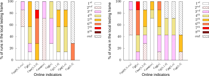
Figure 1: biaf and neuromst model ranking percentages across local testing frames for resource-rich languages

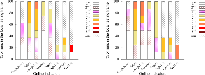
Figure 2: biaf and neuromst model ranking percentages across local testing frames for resource-poor languages

More specifically, for large enough corpora, the biaf models monitored by $c_{\textit{coi}[\aleph,5,\alpha_{\aleph}]}$ achieve the top nemesid scores in most local testing frames (en, es, pl and pt) reflected in Table 3 but three, while it ranked second (fr and ru) and third (de) best in the rest. Regarding the neuromst architecture, the performance is similar, achieving the top nemesid scores in three local testing frames (en, es and fr) included in Table 5, while it ranks second (de, pl and pt) and third (ru) best in the rest.

Comparison with the oracle

Focusing on large enough corpora and using a biaf encoder, $c_{\textit{coi}[\aleph,5,\alpha_{\aleph}]}$ is as accurate as the oracle in two of the local testing frames (en and es), although the difference from the baseline never exceeds two epochs, except for the corpus de, as shown in Table 3. Specifically, in that latter case $c_{\textit{coi}[\aleph,5,\alpha_{\aleph}]}$ stops the learning process far in advance (118 epochs) of the oracle, but with an acceptable cost/benefit trade-off, as is proven by its nemesid score (-0.15). The numbers worsen slightly for the neuromst models which, although never matching the diagnosis of the baseline, are a few iterations away from the oracle in two cases (de and es) and provide good nemesid scores (from -0.10 up to 0.02) in all the other ones (en, fr, pl, pt and ru), as can be seen in Table 5. This translates into a reduction (from 1 up to 86 epochs) of model generation costs except in one case (en), always in combination with a very good cost/benefit trade-off.

As for small corpora and excluding out-of-range runs, our proposal matches the oracle only once when using biaf models (zh), although the difference from the baseline is always negative and does not exceed a few epochs (from 1 up to 9) in other three cases (ca, gl and hi), which means a slight reduction in model generation costs, as shown in Table 4. For the remaining run (sr), $c_{\textit{coi}[\aleph,5,\alpha_{\aleph}]}$ stops the learning process far in advance (192 epochs) of the oracle, but with an acceptable cost/benefit trade-off, as shown in Table 4 through its nemesid score of -0.27. These numbers improve slightly for neuromst models, which match the baseline on two local testing frames (ca and gl) and barely differ in a few epochs (from 1 up to 6 epochs) in three other ones (hi, ja and zh). For the remaining two runs (fa and sr), $c_{\textit{coi}[\aleph,5,\alpha_{\aleph}]}$ stops the learning process far in advance (248 and 224 epochs) of the oracle, with an acceptable cost/benefit trade-off, as can be seen in Table 6 through their nemesid scores (-0.37 and -0.35).

Overview

Overall, we find that the performance of our proposal not only improves on the state-of-the-art, but also comes very close to the oracle, regardless of the architecture applied by the learner or the type of corpus under consideration. All this in operational conditions that are not particularly advantageous for it as we sought the best fit for the rest of the online indicators tested, which is not the case for $c_{\textit{coi}[\aleph,k,\alpha_{\aleph}]}$, whose parameters $\aleph$ and $k$ were set for the occasion without an exhaustive prior tuning process. In particular, the length $k$ of of the training strips, used in our case to delimit the sequence of epochs to be correlated, has been set to the value recommended for the rest of the indicators that apply this type of structure.

6.4.2 The qualitative study

Having confirmed the accuracy of our proposal as tested on a particular configuration, $c_{\textit{coi}[\aleph,k,\alpha_{\aleph}]}$ with $k=5$, we now study its stability, to check whether the good results observed show uniform behavior independent of the resources used, and can also be extrapolated without major variations to other settings. This would allow its use to be simplified, as it would no longer require a cumbersome prior tuning phase.

Stability with regard to the resources

Concerning this, Fig. 3 shows that the nemesid scores for $c_{\textit{coi}[\aleph,5,\alpha_{\aleph}]}$ for the resource-rich languages are the most stable among all the indicators evaluated, independent of the learning architecture used. More to the point, it virtually matches the optimal performance when using a biaf model, excluding the run corresponding to de, which turns out to be an extreme or even an out-of-range run for most indicators. In fact, all the stop conditions exhibit such values, along with –except for $c_{\textit{coi}[\aleph,5,\alpha_{\aleph}]}$ and $c_{\textit{mne}[m]}$– a varying level of asymmetry both in terms of interquartile range and whisker length, revealing an increasing dispersion and variability of the nemesid values.

As for neuromst, although slightly different to those of the oracle, the values for $c_{\textit{coi}[\aleph,5,\alpha_{\aleph}]}$ are still excellent, and the best overall. In greater detail, it shows a mean close to the optimum, with symmetry at the interquartile range and a slight deviation in the whiskers, which show the smallest range and the shortest length respectively. The result is the practical absence of biases in the distribution of nemesid values, with little variability and a high concentration around those of the oracle. In contrast, the impact of the neural architecture is high on the rest of the indicators. Thus, both the size and the asymmetry of interquartile boxes and whiskers increase, while the mean moves away from that of the oracle. Therefore, accuracy and stability degrade significantly with out-of-range runs for half of the indicators, although most of the extreme values have dissapeared with respect to the biaf encoders.

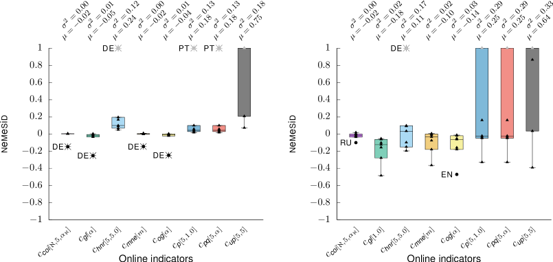
Figure 3: nemesid biaf and neuromst model box plots across local testing frames for resource-rich languages

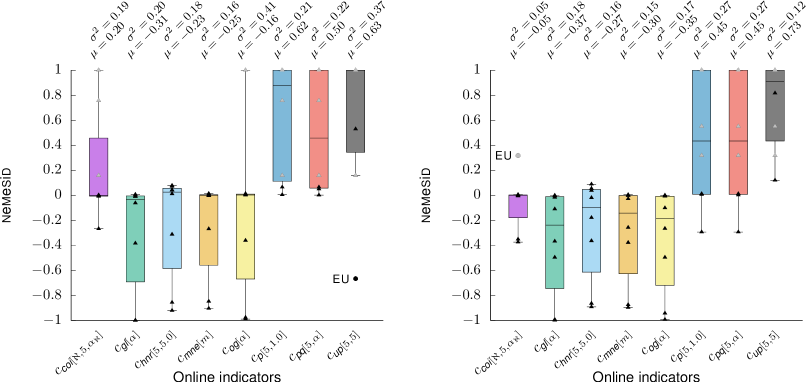
Figure 4: nemesid biaf and neuromst model box plots across local testing frames for resource-poor languages

Regarding the nemesid scores for the resource-poor languages, Fig. 4 shows an increased interquartile range and whisker length for most of the indicators with a worsening of the asymmetry in both cases, which implies the presence of biases. In this respect, $c_{\textit{coi}[\aleph,5,\alpha_{\aleph}]}$ is associated with the most contained distribution, while the symmetry is suffering from the impact of the lack of learning resources, although to a lesser extent than the rest of the indicators studied. The only exception to this generalized behavior is (resp. are) $c_{{\textit{pq}[5,\alpha]}}$ (resp. $c_{\textit{p}[5,1.0]}$ and $c_{{\textit{pq}[5,\alpha]}}$) when using a biaf (resp. neuromst) architecture, but their interquartile ranges and whisker lengths are the highest, which implies a significant dispersion and variability in the performance of the various runs. In contrast to what happened with the sufficiently large corpora, most outliers and extreme values have disappeared here, although the number of out-of-range runs has increased, concentrated mainly among the same indicators as for the large ones.

Stability with regard to the setting

Regarding the stability of $c_{\textit{coi}[\aleph,k,\alpha_{\aleph}]}$ for various settings, we focus on the length $k$ of the training strip since the tuning of the threshold $\alpha_{\aleph}$ for each local testing frame had already been described, and we assume that the impact of the concrete correlation coefficient $\aleph$ used is comparatively minor in regulating the learning process. Bearing in mind that a correct strip must have a length of at least 2, we compare the nemesid values obtained for $k=2,5$ and $8$, ensuring a symmetric analysis. Once again taking cross-validation as the canary function $c$, we introduce the collection $\Upsilon_{c}^{\textit{coi}}$ of online indicators to be considered as:

$$\Upsilon_{c}^{\textit{coi}}:=\{c_{\textit{coi}[\aleph,2,\alpha_{\aleph}]},c_{\textit{coi}[\aleph,5,\alpha_{\aleph}]},c_{\textit{coi}[\aleph,8,\alpha_{\aleph}]}\}$$ (31)

together with the neural architectures (biaf and neuromst) and the ud treebank collections ($R$ and $P$) as already identified. We then define the local testing frame families as:

$$\{\mathcal{L}_{R,d}^{\Upsilon_{c}^{\textit{coi}}}\}_{d\in{\mathcal{D}}}\mbox{ (resp. }\{\mathcal{L}_{P,d}^{\Upsilon_{c}^{\textit{coi}}}\}_{d\in{\mathcal{D}}}\mbox{)},\mbox{ with }{\mathcal{D}}:=\{\mbox{{\sc b}i{\sc af}},\mbox{{\sc n}euro{\sc mst}}\}$$ (32)

one per combination of corpus in $R$ (resp. $P$) and encoder $d\in{\mathcal{D}}$. Those families, together with the nemesid quality metric make up our new experimental environment.

		$c_{\textit{coi}[\aleph,2,\alpha_{\aleph}]}$						$c_{\textit{coi}[\aleph,5,\alpha_{\aleph}]}$						$c_{\textit{coi}[\aleph,8,\alpha_{\aleph}]}$								$c_{\textit{coi}[\aleph,2,\alpha_{\aleph}]}$						$c_{\color[rgb]{.5,0,.5}\textit{coi}[\aleph,5,\alpha_{\aleph}]}$						$c_{\textit{coi}[\aleph,8,\alpha_{\aleph}]}$
		$\alpha_{\aleph}$		$s_{c_{\textit{coi}[\aleph,2,\alpha_{\aleph}]}}$		$\Phi_{0.5}^{0.5}$		$\alpha_{\aleph}$		$s_{c_{\textit{coi}[\aleph,5,\alpha_{\aleph}]}}$		$\Phi_{0.5}^{0.5}$		$\alpha_{\aleph}$		$s_{c_{\textit{coi}[\aleph,8,\alpha_{\aleph}]}}$		$\Phi_{0.5}^{0.5}$				$\alpha_{\aleph}$		$s_{c_{\textit{coi}[\aleph,2,\alpha_{\aleph}]}}$		$\Phi_{0.5}^{0.5}$		$\alpha_{\aleph}$		$s_{c_{\textit{coi}[\aleph,5,\alpha_{\aleph}]}}$		$\Phi_{0.5}^{0.5}$		$\alpha_{\aleph}$		$s_{c_{\textit{coi}[\aleph,8,\alpha_{\aleph}]}}$		$\Phi_{0.5}^{0.5}$
de		0.5		196		-0.01		0.5		88		-0.15		0.5		92		-0.14		ca		0.5		40		-0.03		0.7		55		-0.01		0.7		58		-0.01
en		0.5		41		0.00		0.5		41		0.00		0.5		46		0.01		eu		0.5		$10^{3}$		0.76		1.0		$10^{3}$		0.76		1.0		$10^{3}$		0.76
es		0.5		42		0.00		0.5		42		0.00		0.5		43		0.00		fa		1.0		$10^{3}$		0.16		1.0		$10^{3}$		0.16		1.0		$10^{3}$		0.16
fr		0.5		4		0.00		0.5		5		0.00		0.5		8		0.01		gl		0.5		19		-0.00		0.5		19		-0.00		0.5		17		-0.00
pl		0.5		20		-0.00		0.5		21		-0.00		0.5		22		0.00		hi		0.5		10		-0.01		0.5		13		-0.00		0.5		16		-0.00
pt		0.5		27		0.00		0.7		29		0.00		0.5		23		-0.00		ja		1.0		$10^{3}$		1.00		1.0		$10^{3}$		1.00		1.0		$10^{3}$		1.00
ru		0.5		14		0.00		0.5		16		0.00		0.5		8		-0.01		sr		0.5		264		-0.03		0.5		92		-0.27		0.5		90		-0.27
																				zh		0.5		5		0.00		0.5		5		0.00		0.5		8		0.01

Table 7: biaf encoder monitoring of local testing frames with $c_{\textit{coi}[\aleph,k,\alpha_{\aleph}]}$ for resource-rich and resource-poor languages

		$c_{\textit{coi}[\aleph,2,\alpha_{\aleph}]}$						$c_{\textit{coi}[\aleph,5,\alpha_{\aleph}]}$						$c_{\textit{coi}[\aleph,8,\alpha_{\aleph}]}$								$c_{\textit{coi}[\aleph,2,\alpha_{\aleph}]}$						$c_{\color[rgb]{.5,0,.5}\textit{coi}[\aleph,5,\alpha_{\aleph}]}$						$c_{\textit{coi}[\aleph,8,\alpha_{\aleph}]}$
		$\alpha_{\aleph}$		$s_{c_{\textit{coi}[\aleph,2,\alpha_{\aleph}]}}$		$\Phi_{0.5}^{0.5}$		$\alpha_{\aleph}$		$s_{c_{\textit{coi}[\aleph,5,\alpha_{\aleph}]}}$		$\Phi_{0.5}^{0.5}$		$\alpha_{\aleph}$		$s_{c_{\textit{coi}[\aleph,8,\alpha_{\aleph}]}}$		$\Phi_{0.5}^{0.5}$				$\alpha_{\aleph}$		$s_{c_{\textit{coi}[\aleph,2,\alpha_{\aleph}]}}$		$\Phi_{0.5}^{0.5}$		$\alpha_{\aleph}$		$s_{c_{\textit{coi}[\aleph,5,\alpha_{\aleph}]}}$		$\Phi_{0.5}^{0.5}$		$\alpha_{\aleph}$		$s_{c_{\textit{coi}[\aleph,8,\alpha_{\aleph}]}}$		$\Phi_{0.5}^{0.5}$
de		0.5		71		0.01		0.5		61		-0.01		0.5		60		-0.01		ca		0.5		261		-0.02		0.5		277		0.00		1.0		283		0.01
en		0.5		343		0.01		0.5		345		0.02		0.7		319		-0.02		eu		0.5		$10^{3}$		0.32		0.5		$10^{3}$		0.32		0.5		$10^{3}$		0.32
es		0.5		71		0.00		0.5		70		-0.00		0.6		67		-0.00		fa		0.5		91		-0.38		0.5		94		-0.37		1.0		343		0.00
fr		0.5		208		-0.03		0.5		208		-0.03		0.5		261		0.04		gl		0.5		114		-0.00		0.5		117		0.00		0.5		18		-0.11
pl		0.5		85		-0.02		0.5		85		-0.02		0.8		103		0.00		hi		0.5		17		-0.01		0.5		28		0.00		0.8		17		-0.01
pt		0.5		80		-0.05		0.5		88		-0.04		0.5		88		-0.04		ja		0.5		5		-0.00		0.5		5		-0.00		0.5		8		0.00
ru		0.5		90		-0.08		0.5		70		-0.10		0.5		60		-0.11		sr		0.5		$10^{3}$		0.55		0.7		425		-0.35		1.0		439		-0.33
																				zh		0.5		3		-0.01		0.5		24		-0.01		0.5		20		-0.01

Table 8: neuromst encoder monitoring of local testing frames with $c_{\textit{coi}[\aleph,k,\alpha_{\aleph}]}$ for resource-rich and resource-poor languages

The rows in Tables 7 and 8 reflect the results for the local testing frames in $\{\mathcal{L}_{R,d}^{\Upsilon_{c}^{\textit{coi}}},\mathcal{L}_{P,d}^{\Upsilon_{c}^{\textit{coi}}}\}_{d\in{\mathcal{D}}}$, and their entries show the runs associated with indicators in the collection $\Upsilon_{c}^{\textit{coi}}$ following the same pattern applied in previous tests. Meanwhile, Figs. 5 and 6 summarize the distributions of nemesid values associated with those runs, differentiating between the biaf (left-hand side) and the neuromst (right-hand side) encodings for the resource-rich and resource-poor languages, respectively.

Figure 5: nemesid biaf and neuromst model box plots across coi-based local testing frames for resource-rich languages

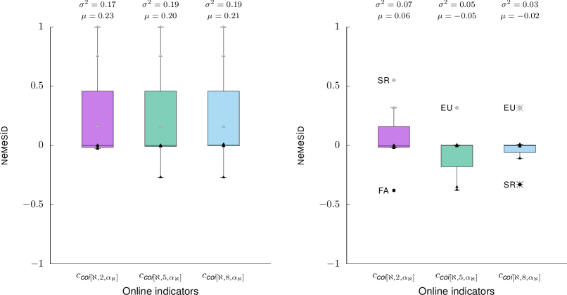
Figure 6: nemesid biaf and neuromst model box plots across coi-based local testing frames for resource-poor languages

Our proposal shows rock-solid stability for resource-rich languages, with nemesid values ranging over the interval $[-0.15,0.01]$ (resp. $[-0.11,0.04]$) for the biaf (resp. neuromst) architecture, independent of the value $k\in\{2,5,8\}$ considered for the length of the training strip, as reflected in the left-hand-side of Table 7 (resp. Table 8), although the best results are associated with $k=2$. Thus, the interquartile range, whisker length and symmetry have no, or only minor, fluctuations. Only the neuromst models suffer a slight degradation in the symmetry for the highest values of $k$, which involves the whisker lengths for $k=5$, and both interquartile range and whisker lengths for $k=8$. The presence of one extreme value for the biaf encoders can be considered to be irrelevant and is once again associated with the de corpus, as was the case for most of the state-of-the-art indicators already studied. This suggests that the origin of the phenomenon may lie to some extent in the nature of the training database. Along the same lines, we can also consider the characterization as an outlier of the run corresponding to the corpus ru when using neuromst, for the cases $k=5$ and $k=8$, as not very relevant.

Stability parameters worsen slightly for smaller corpora, if we exclude out-of-range runs, with nemesid values ranging over the interval $[-0.27,0.01]$ (resp. $[-0.38,0.01]$) for biaf (resp. neuromst) models, independent of the value $k$ considered. On the other hand, and in contrast to what happened for the larger corpora, the impact of architecture seems to be decisive here. As for the distribution parameters, the impact of out-of-range runs in the biaf architecture is visible, to which must be added those associated with outliers and extreme values when using neuromst encoders. For the biaf case, this impact is practically the same for all the various training strip lengths considered, in terms of interquartile box, whiskers and symmetry considerations. The only exception to this uniform behavior is the length of the lower whisker for $c_{{\textit{coi}[\aleph,2,\alpha\aleph]}}$, which is more closely matched to the mean. In contrast, neuromst models show a more contained dispersion at all levels, but are also less uniform, with the best distribution parameters associated with $c_{{\textit{coi}[\aleph,8,\alpha\aleph]}}$, although the best individual results are now concentrated on indicator $c_{{\textit{coi}[\aleph,5,\alpha\aleph]}}$.

Overview

Overall, the results show a remarkable stability in the treatment of both resource-intensive and resource-scarce languages, the latter being more dependent on the learning architecture used. The fact that in most cases the behavior improves for reduced lengths ($k=2$) would suggest that the configuration $k=5$ used in our previous comparison with the state-of-the-art is not optimal, thus giving greater value to the results previously discussed.

7 Conclusions

We have formally described an early stopping technique to anticipate overfitting in dl-based learning, exploiting cross-validation as the predictive basis. The novelty compared to previous work lies in formally tackling two key issues: the specification of early stopping criteria and the interpretation of agreement among these. In the first case, we have described a well-defined framework based on the notion of the canary function from gp, using online indicators to warn of overfitting. In the second case, we have analyzed the agreement in the diagnosis from the perspective of the pcc, thus giving theoretical support to our decision-making.

Our case study focused on the particularly complex task of generating nlp parsers. The results indicate that our proposal improves generalization capabilities while increasing learning efficiency and reducing sensitivity with respect to parameter choice. This shows the potential of correlating decision criteria as a means of providing stability and preventing overfitting during model training.

References

- Amari et al. (1997) Amari, S.-I., Murata, N., Müller, K.-R., Finke, M., Yang, H. H., 1997. Asymptotic statistical theory of overtraining and cross-validation. IEEE Transactions on Neural Networks 8 (5), 985–996.
- Arntzenius (1993) Arntzenius, F., 1993. The common cause principle. PSA 1992, 227–237.
- Arntzenius (2010) Arntzenius, F., 2010. Reichenbach’s common cause principle. In: Zalta, E. N. (Ed.), The Stanford Encyclopedia of Philosophy, fall 2010 Edition. Metaphysics Research Lab, Stanford University.
- Baldi and Chauvin (1991) Baldi, P., Chauvin, Y., 1991. Temporal evolution of generalization during learning in linear networks. Neural Computation 3 (4), 589–603.
- Bengio et al. (2013) Bengio, Y., Courville, A., Vincent, P., 2013. Representation learning: A review and new perspectives. IEEE Transactions on Pattern Analysis and Machine Intelligence 35 (8), 1798–1828.
- Bianchini and Scarselli (2014) Bianchini, M., Scarselli, F., 2014. On the complexity of neural network classifiers: A comparison between shallow and deep architectures. IEEE Transactions on Neural Networks and Learning Systems 25 (8), 1553–1565.
- Bishop (1995) Bishop, C., 1995. Regularization and complexity control in feed-forward networks. In: Fougelman-Soulie, F., Gallinari, P. (Eds.), Proceedings International Conference on Artificial Neural Networks. Vol. 1 of ICANN’95. pp. 141–148.
- Blanchard and Krämer (2010) Blanchard, G., Krämer, N., 2010. Optimal learning rates for kernel conjugate gradient regression. In: Lafferty, J., Williams, C., Shawe-Taylor, J., Zemel, R., Culotta, A. (Eds.), Advances in Neural Information Processing Systems 23. Curran Associates, Inc., pp. 226–234.
- Blanchard and Mücke (2018) Blanchard, G., Mücke, N., 2018. Optimal rates for regularization of statistical inverse learning problems. Foundations of Computational Mathematics 18 (4), 971–1013.
- Buchholz and Marsi (2006) Buchholz, S., Marsi, E., 2006. CoNLL-X shared task on multilingual dependency parsing. In: 10th Conference on Computational Natural Language Learning. New York, pp. 149–164.
- Buhlmann and Yu (2003) Buhlmann, P., Yu, B., 2003. Boosting with the l2 loss: Regression and classification. Journal of the American Statistical Association 98, 324–339.
- Cartwright (1979) Cartwright, N., 1979. Causal laws and effective strategies. Noûs 13 (4), 419–437.
- Cartwright (1988) Cartwright, N., 01 1988. How to Tell a Common Cause: Generalizations of the Conjunctive Fork Criterion. pp. 181–188.
- Cataltepe et al. (1999) Cataltepe, Z., Abu-Mostafa, Y. S., Magdon-Ismail, M., 1999. No free lunch for early stopping. Neural Computation 11 (4), 995–1009.
- Coates et al. (2013) Coates, A., Huval, B., Wang, T., Wu, D. J., Ng, A. Y., Catanzaro, B., 2013. Deep learning with cots hpc systems. In: 30th International Conference on International Conference on Machine Learning - Volume 28. ICML’13. JMLR.org, pp. III–1337–III–1345.
- Collobert et al. (2011) Collobert, R., Weston, J., Bottou, L., Karlen, M., Kavukcuoglu, K., Kuksa, P., 2011. Natural language processing (almost) from scratch. Journal of Machine Learning Research 12, 2493–2537.
- Culotta and Sorensen (2004) Culotta, A., Sorensen, J., 2004. Dependency tree kernels for relation extraction. In: 42nd Annual Meeting of the Association for Computational Linguistics. ACL’04. Barcelona, Spain, pp. 423–429.
- de Marneffe et al. (2014) de Marneffe, M.-C., Dozat, T., Silveira, N., Haverinen, K., Ginter, F., Nivre, J., Manning, C. D., 2014. Universal Stanford dependencies: A cross-linguistic typology. In: Ninth International Conference on Language Resources and Evaluation. LREC’14. European Language Resources Association (ELRA), Reykjavik, Iceland, pp. 4585–4592.
- Ding and Palmer (2005) Ding, Y., Palmer, M., 2005. Machine translation using probabilistic synchronous dependency insertion grammars. In: 43rd Annual Meeting of the Association for Computational Linguistics. ACL’05. Association for Computational Linguistics, Ann Arbor, Michigan, pp. 541–548.
- Dodier (1996) Dodier, R., 1996. Geometry of early stopping in linear networks. In: Advances in Neural Information Processing Systems. The MIT Press, pp. 365–371.
- Dozat and Manning (2017) Dozat, T., Manning, C. D., 2017. Deep biaffine attention for neural dependency parsing. In: 5th International Conference on Learning Representations. ICLR’17. OpenReview.net, Toulon, France, pp. 24–26.
- Eells (1991) Eells, E., 1991. Probabilistic Causality. Cambridge Studies in Probability, Induction and Decision Theory. Cambridge University Press.
- Evett et al. (1998) Evett, M., Khoshgoftar, T., der Chien, P., Allen, E., 1998. GP-based software quality prediction. In: Koza, J. R., Banzhaf, W., Chellapilla, K., Deb, K., Dorigo, M., Fogel, D. B., Garzon, M. H., Goldberg, D. E., Iba, H., Riolo, R. (Eds.), Genetic Programming 1998: Third Annual Conference. Morgan Kaufmann, University of Wisconsin, Madison, Wisconsin, USA, pp. 60–65.
- Fahlman and Lebiere (1990) Fahlman, S. E., Lebiere, C., 1990. Advances in neural information processing systems 2. Morgan Kaufmann Publishers Inc., San Francisco, CA, USA, Ch. The Cascade-correlation Learning Architecture, pp. 524–532.
- Faruqui et al. (2015) Faruqui, M., Dodge, J., Jauhar, S. K., Dyer, C., Hovy, E., Smith, N. A., 2015. Retrofitting word vectors to semantic lexicons. In: 2015 Conference of the North American Chapter of the Association for Computational Linguistics: Human Language Technologies. Association for Computational Linguistics, Denver, Colorado, pp. 1606–1615.
- Finnoff et al. (1993) Finnoff, W., Hergert, F., Zimmermann, H. G., 1993. Improving model selection by nonconvergent methods. Neural Networks 6 (6), 771–783.
- Foreman and Evett (2005) Foreman, N., Evett, M., 2005. Preventing overfitting in GP with canary functions. In: 7th Annual Conference on Genetic and Evolutionary Computation. GECCO ’05. ACM, New York, NY, USA, pp. 1779–1780.
- Forster (2014) Forster, M. R., 2014. The principle of common cause. In: Friel Gutting, A. (Ed.), Notre Dame Philosophical Reviews. College of Arts and Letters, University of Notre Dame.
- Geman et al. (1992) Geman, S., Bienenstock, E., Doursat, R., 1992. Neural networks and the bias/variance dilemma. Neural Computation 4 (1), 1–58.
- Goldberg and Hirst (2017) Goldberg, Y., Hirst, G., 2017. Neural Network Methods in Natural Language Processing. Morgan & Claypool Publishers.
- Goodfellow et al. (2016) Goodfellow, I., Bengio, Y., Courville, A., 2016. Deep Learning. The MIT Press.
- Hassibi and Stork (1993) Hassibi, B., Stork, D. G., 1993. Second order derivatives for network pruning: Optimal brain surgeon. In: Advances in Neural Information Processing Systems 5, [NIPS Conference]. Morgan Kaufmann Publishers Inc., San Francisco, CA, USA, pp. 164–171.
- Hinton (1989) Hinton, G. E., 1989. Connectionist learning procedures. Artificial Intelligence 40 (1-3), 185–234.
- Hitchcock (2012) Hitchcock, C., 2012. Probabilistic causation. In: Zalta, E. N. (Ed.), Stanford Encyclopedia of Philosophy.
- Hofer-Szabó et al. (1998) Hofer-Szabó, G., Rédei, M., Szabó, L. E., 06 1998. On reichenbach’s common cause principle and reichenbach’s notion of common cause. British Journal for the Philosophy of Science 50.
- Hofer-Szabó et al. (2013) Hofer-Szabó, G., Rédei, M., Szabó, L. E., 2013. The Common Cause Principle. Cambridge University Press, pp. 11–17.
- Holmstrom and Koistinen (1992) Holmstrom, L., Koistinen, P., Jan 1992. Using additive noise in back-propagation training. IEEE Transactions on Neural Networks 3 (1), 24–38.
- Hume (1904) Hume, D., 1904. Enquiry Concerning Human Understanding. Clarendon Press.
- Jones (1994) Jones, K. S., 1994. Natural Language Processing: A Historical Review. Springer Netherlands, Dordrecht, pp. 3–16.
- Jurafsky and Martin (2009) Jurafsky, D., Martin, J. H., 2009. Speech and Language Processing: An Introduction to Natural Language Processing, Computational Linguistics, and Speech Recognition. Prentice Hall Series in Artificial Intelligence. Pearson Prentice Hall, Upper Saddle River.
- Kim et al. (2018) Kim, J.-H., Jun, J., Zhang, B.-T., 2018. Bilinear attention networks. In: Bengio, S., Wallach, H., Larochelle, H., Grauman, K., Cesa-Bianchi, N., Garnett, R. (Eds.), Advances in Neural Information Processing Systems. Vol. 31. Curran Associates, Inc., pp. 1564–1574.
- Krogh and Hertz (1992) Krogh, A., Hertz, J. A., 1992. A simple weight decay can improve generalization. In: Moody, J. E., Hanson, S. J., Lippmann, R. P. (Eds.), Advances in Neural Information Processing Systems 4. San Francisco, CA: Morgan Kaufmann, pp. 950–957.
- Kubler et al. (2009) Kubler, S., McDonald, R., Nivre, J., Hirst, G., 2009. Dependency Parsing. Morgan and Claypool Publishers.
- LeCun and Bengio (1998) LeCun, Y., Bengio, Y., 1998. Convolutional Networks for Images, Speech, and Time Series. MIT Press, Cambridge, MA, USA, pp. 255–258.
- LeCun et al. (2015) LeCun, Y., Bengio, Y., Hinton, G., 2015. Deep learning. Nature Cell Biology 521 (7553), 436–444.
- Liu et al. (2019) Liu, L., Lin, X., Joty, S., Han, S., Bing, L., 2019. Hierarchical pointer net parsing. In: 2019 Conference on Empirical Methods in Natural Language Processing and the 9th International Joint Conference on Natural Language Processing. EMNLP-IJCNLP’19. Association for Computational Linguistics, Hong Kong, China, pp. 1007–1017.
- Liu et al. (2008) Liu, Y., Starzyk, J., Zhu, Z., 2008. Optimized approximation algorithm in neural networks without overfitting. IEEE Transactions on Neural Networks 19 (6), 983–995.
- Lodwich et al. (2009) Lodwich, A., Rangoni, Y., Breuel, T., 2009. Evaluation of robustness and performance of early stopping rules with multi layer perceptrons. In: 2009 International Joint Conference on Neural Networks. IJCNN’09. IEEE Press, Piscataway, NJ, USA, pp. 333–340.
- Ma and Hovy (2016) Ma, X., Hovy, E., Aug. 2016. End-to-end sequence labeling via bi-directional LSTM-CNNs-CRF. In: 54th Annual Meeting of the Association for Computational Linguistics (Volume 1: Long Papers). Association for Computational Linguistics, Berlin, Germany, pp. 1064–1074.
- Ma and Hovy (2017) Ma, X., Hovy, E., 2017. Neural probabilistic model for non-projective MST parsing. In: Eighth International Joint Conference on Natural Language Processing (Volume 1: Long Papers). IJCNLP’17. Asian Federation of Natural Language Processing, Taipei, Taiwan, pp. 59–69.
- Ma et al. (2018) Ma, X., Hu, Z., Liu, J., Peng, N., Neubig, G., Hovy, E., 2018. Stack-pointer networks for dependency parsing. In: 56th Annual Meeting of the Association for Computational Linguistics (Volume 1: Long Papers). ACL’18. Association for Computational Linguistics, Melbourne, Australia, pp. 1403–1414.
- Magnini et al. (2020) Magnini, B., Lavelli, A., Magnolini, S., 2020. Comparing machine learning and deep learning approaches on NLP tasks for the Italian language. In: 12th Language Resources and Evaluation Conference. European Language Resources Association, Marseille, France, pp. 2110–2119.
- Manning (2015) Manning, C. D., 2015. Computational linguistics and deep learning. Computational Linguistics 41 (4), 701–707.
- McCulloch and Pitts (1988) McCulloch, W. S., Pitts, W., 1988. Neurocomputing: Foundations of research. MIT Press, Cambridge, MA, USA, Ch. A Logical Calculus of the Ideas Immanent in Nervous Activity, pp. 15–27.
- Meek et al. (2002) Meek, C., Thiesson, B., Heckerman, D., Mar. 2002. The learning-curve sampling method applied to model-based clustering. The Journal of Machine Learning Research 2, 397–418.
- Michalak and Raciborski (2005) Michalak, K., Raciborski, R., 2005. Dynamic correlation approach to early stopping in artificial neural network training. macroeconomic forecasting example. In: 5th International Conference on Intelligent Systems Design and Applications. ISDA ’05. IEEE Computer Society, Washington, DC, USA, pp. 100–105.
- Mikolov et al. (2010) Mikolov, T., Karafiát, M., Burget, L., Cernocký, J., Khudanpur, S., 2010. Recurrent neural network based language model. In: Kobayashi, T., Hirose, K., Nakamura, S. (Eds.), Interspeech. Vol. 2. ISCA, pp. 1045–1048.
- Mill (1868) Mill, J. S., 1868.
- Morgan and Bourlard (1990) Morgan, N., Bourlard, H., 1990. Advances in neural information processing systems 2. Morgan Kaufmann Publishers Inc., San Francisco, CA, USA, Ch. Generalization and Parameter Estimation in Feedforward Nets: Some Experiments, pp. 630–637.
- Nguyen et al. (2012) Nguyen, T. H., Nguyen, X. H., McKay, B., Nguyen, Q. U., 2012. Where should we stop? an investigation on early stopping for GP learning. In: 9th International Conference on Simulated Evolution and Learning. SEAL’12. Springer-Verlag, Berlin, Heidelberg, pp. 391–399.
- Nilsson (1990) Nilsson, N. J., 1990. The Mathematical Foundations of Learning Machines. Morgan Kaufmann Publishers Inc., San Francisco, CA, USA.
- Nowlan and Hinton (1992) Nowlan, S. J., Hinton, G. E., 1992. Simplifying neural networks by soft weight-sharing. Neural Computation 4 (4), 473–493.
- Pearson (1895) Pearson, K., 1895. Note on regression and inheritance in the case of two parents. Proceedings of the Royal Society of London 58, 240–242.
- Piotrowski and Napiorkowski (2013) Piotrowski, A. P., Napiorkowski, J. J., 2013. A comparison of methods to avoid overfitting in neural networks training in the case of catchment runoff modelling. Journal of Hydrology 476 (Complete), 97–111.
- Plank and Klerke (2019) Plank, B., Klerke, S., 2019. Lexical resources for low-resource PoS tagging in neural times. In: 22nd Nordic Conference on Computational Linguistics. Linköping University Electronic Press, Turku, Finland, pp. 25–34.
- Pólya (1920) Pólya, G., 1920. Uber den zentralen grenzwertsatz der wahrscheinlichkeitsrechnung und das momentenproblem. Mathematische Zeitschrift 8, 171–181.
- Prechelt (1997) Prechelt, L., 1997. Automatic early stopping using cross validation: Quantifying the criteria. Neural Networks 11, 761–767.
- Raina et al. (2009) Raina, R., Madhavan, A., Ng, A. Y., 2009. Large-scale deep unsupervised learning using graphics processors. In: 26th Annual International Conference on Machine Learning. ICML ’09. ACM, New York, NY, USA, pp. 873–880.
- Raskutti et al. (2014) Raskutti, G., Wainwright, M. J., Yu, B., 2014. Early stopping and non-parametric regression: An optimal data-dependent stopping rule. Journal of Machine Learning Research 15 (1), 335–366.
- Reichenbach (1956) Reichenbach, H., 1956. The Direction of Time. Dover Publications.
- Rosasco and Villa (2015) Rosasco, L., Villa, S., 2015. Learning with incremental iterative regularization. In: Cortes, C., Lawrence, N. D., Lee, D. D., Sugiyama, M., Garnett, R. (Eds.), Advances in Neural Information Processing Systems 28. Curran Associates, Inc., pp. 1630–1638.
- Rotman and Reichart (2019) Rotman, G., Reichart, R., Mar. 2019. Deep contextualized self-training for low resource dependency parsing. Transactions of the Association for Computational Linguistics 7, 695–713.
- Rumelhart et al. (1986) Rumelhart, D., Hinton, G., Williams, R., 1986. Parallel distributed processing: Explorations in the microstructure of cognition, vol. 1. MIT Press, Cambridge, MA, USA, Ch. Learning Internal Representations by Error Propagation, pp. 318–362.
- Russell (1948) Russell, B., 1948. Human Knowledge: Its Scope and Limits. Simon and Schuster.
- Sagae (2009) Sagae, K., 2009. Analysis of discourse structure with syntactic dependencies and data-driven shift-reduce parsing. In: 11th International Conference on Parsing Technologies. IWPT’09. Association for Computational Linguistics, Paris, France, pp. 81–84.
- Salmon (1984) Salmon, W., 1984. Scientific Explanation and the Causal Structure of the World. LPE Limited Paperback Editions. Princeton University Press.
- Sampson and McCarthy (2004) Sampson, G., McCarthy, D., 2004. Corpus linguistics: readings in a widening discipline. Open linguistics series. Continuum.
- San Pedro and Suárez (2009) San Pedro, I., Suárez, M., 2009. Reichenbach’s common cause principle and indeterminism: A review. In: Recio, J. L. G. (Ed.), Philosophical Essays on Physics and Biology. Georg Olms Verlag, pp. 223–250.
- Schmidhuber (2015) Schmidhuber, J., 2015. Deep learning in neural networks. Neural Networks 61 (C), 85–117.
- Shao et al. (2011) Shao, Y., Taff, G. N., Walsh, S. J., Jan 2011. Comparison of early stopping criteria for neural-network-based subpixel classification. IEEE Geoscience and Remote Sensing Letters 8 (1), 113–117.
- Shinyama et al. (2002) Shinyama, Y., Sekine, S., Sudo, K., 2002. Automatic paraphrase acquisition from news articles. In: Second International Conference on Human Language Technology Research. HLT’02. Morgan Kaufmann Publishers Inc., San Francisco, CA, USA, pp. 313–318.
- Sjöberg and Ljung (1995) Sjöberg, J., Ljung, L., 1995. Overtraining, regularization and searching for a minimum, with application to neural networks. International Journal of Control 62 (6), 1391–1407.
- Skyrms (1981) Skyrms, B., 1981. Causal necessity. Philosophy of Science 48 (2), 329–335.
- Spearman (1904) Spearman, C., 1904. The proof and measurement of association between two things. American Journal of Psychology 15, 88–103.
- Suppes (1970) Suppes, P., 1970. A Probabilistic Theory of Causality. Amsterdam: North-Holland Pub. Co.
- Tesnière (1959) Tesnière, L., 1959. Eléments de Syntaxe Structurale. Klincksieck, Paris.
- Tourille et al. (2018) Tourille, J., Doutreligne, M., Ferret, O., Névéol, A., Paris, N., Tannier, X., Oct. 2018. Evaluation of a sequence tagging tool for biomedical texts. In: Ninth International Workshop on Health Text Mining and Information Analysis. Association for Computational Linguistics, Brussels, Belgium, pp. 193–203.
- Tuite et al. (2011) Tuite, C., Agapitos, A., O’Neill, M., Brabazon, A., 2011. Early stopping criteria to counteract overfitting in genetic programming. In: 13th Annual Conference Companion on Genetic and Evolutionary Computation. GECCO ’11. ACM, New York, NY, USA, pp. 203–204.
- Van Fraassen (1982) Van Fraassen, B., 1982. Rational belief and the common cause principle. In: McLaughlin, R. (Ed.), What? Where? When? Why? Essays in Honour of Wesley Salmon. Reidel, Dordrecht, pp. 193–209.
- Vanneschi et al. (2010) Vanneschi, L., Castelli, M., Silva, S., 2010. Measuring bloat, overfitting and functional complexity in genetic programming. In: 12th Annual Conference on Genetic and Evolutionary Computation. GECCO ’10. ACM, New York, NY, USA, pp. 877–884.
- Wang et al. (1994) Wang, C., Venkatesh, S., Judd, J., 1994. Optimal stopping and effective machine complexity in learning. In: Cowan, J., Tesauro, G., Alspector, J. (Eds.), Advances in Neural Information Processing Systems 6. San Francisco, CA: Morgan Kaufmann, pp. 303–310.
- Wang and Yan (2017) Wang, W., Yan, X.-F., 2017. Early stopping criterion combining probability density function with validation error for improving the generalization capability of the backpropagation neural network. In: 2nd International Conference on Applied Mechanics and Mechatronics Engineering. AMME’17. Shanghai, China, pp. 205–209.
- Wei et al. (2017) Wei, Y., Yang, F., Wainwright, M. J., 2017. Early stopping for kernel boosting algorithms: A general analysis with localized complexities. In: Guyon, I., Luxburg, U. V., Bengio, S., Wallach, H., Fergus, R., Vishwanathan, S., Garnett, R. (Eds.), Advances in Neural Information Processing Systems 30. Curran Associates, Inc., pp. 6065–6075.
- Weiss and Tian (2008) Weiss, G., Tian, Y., 2008. Maximizing classifier utility when there are data acquisition and modeling costs. Data Mining and Knowledge Discovery 17 (2), 253–282.
- Yao et al. (2007) Yao, Y., Rosasco, L., Caponnetto, A., Aug 2007. On early stopping in gradient descent learning. Constructive Approximation 26 (2), 289–315.
- Young et al. (2018) Young, T., Hazarika, D., Poria, S., Cambria, E., 08 2018. Recent trends in deep learning based natural language processing. IEEE Computational Intelligence Magazine 13, 55–75.
- Zhang and Yu (2005) Zhang, T., Yu, B., 2005. Boosting with early stopping: Convergence and consistency. Annals of Statistics 33 (4), 1538–1579.