Addressing the Hubble tension in Yukawa cosmology?

Abstract

In Yukawa cosmology, a recent discovery revealed a relationship between baryonic matter and the dark sector. The relationship is described by the parameter $\alpha$ and the long-range interaction parameter $\lambda$ - an intrinsic property of the graviton. Applying the uncertainty relation to the graviton raises a compelling question: Is there a quantum mechanical limit to the measurement precision of the Hubble constant ($H_{0}$)? We argue that the uncertainty relation for the graviton wavelength $\lambda$ can be used to explain a running of $H_{0}$ with redshift. We show that the uncertainty in time has an inverse correlation with the value of the Hubble constant. That means that the measurement of the Hubble constant is intrinsically linked to length scales (redshift) and is connected to the uncertainty in time. On cosmological scales, we found that the uncertainty in time is related to the look-back time quantity. For measurements with a high redshift value, there is more uncertainty in time, which leads to a smaller value for the Hubble constant. Conversely, there is less uncertainty in time for local measurements with a smaller redshift value, resulting in a higher value for the Hubble constant. Therefore, due to the uncertainty relation, the Hubble tension is believed to arise from fundamental limitations inherent in cosmological measurements.

I Introduction

The Hubble tension is a well-known problem in modern cosmology. This problem arises from a discrepancy in the measurements of the Hubble constant $H_{0}$, which describes the rate at which the current Universe is expanding (see Vagnozzi (2023, 2020); Di Valentino et al. (2020)). On the one hand, we have measurements for the $H_{0}$ that are based on observations of objects in our local Universe, say Cepheid variable stars and Type Ia supernovae Riess et al. (2022); on the other hand, we have the measurements on $H_{0}$ based on the Cosmic Microwave Background (CMB) radiation left over from the Big Bang, which provides a snapshot of the early universe Aghanim et al. (2020). The tension arises because these two methods yield different results for $H_{0}$. Observations from the local Universe give a higher value for the Hubble constant compared to predictions based on the CMB and the standard model of cosmology. Based on current observations, the prevailing cosmological model depicts our Universe as homogeneous and isotropic on large scales. A particularly intriguing revelation is the existence of cold dark matter, an enigmatic form of matter that interacts solely through gravitational forces Peebles (1984); Bond and Efstathiou (1984); Trimble (1987); Turner (1991). Despite numerous attempts, the direct detection of dark matter particles continues to be challenging, and its existence is only inferred through the gravitational effects it imparts on galaxies and broader cosmic structures Salucci et al. (2021). In addition to the mysteries surrounding dark matter, dark energy has been introduced to explain the observed accelerated expansion of the Universe, as highlighted by multiple independent observations. This dark energy is closely associated with the cosmological constant (Carroll et al., 1992; Perlmutter et al., 1998; Riess et al., 1998; Peebles and Ratra, 2003). The theoretical framework that comprehensively describes the observed cosmological phenomena is the $\Lambda$CDM paradigm, the most successful model in modern cosmology. However, fundamental questions persist regarding the nature and behaviour of dark matter and dark energy Weinberg (1989); Zlatev et al. (1999); Padmanabhan (2003). A deep understanding of the Universe’s physical depiction remains elusive even though scalar fields are introduced, as in the inflationary scenario, (Starobinsky, 1980; Guth, 1981; D’Agostino and Luongo, 2022; D’Agostino et al., 2022; Capozziello and Shokri, 2022). Recent inconsistencies among cosmological datasets have underscored tensions within the standard $\Lambda$CDM model, prompting questions about its accuracy in describing the entire evolution and dynamics of the universe Di Valentino et al. (2021); Perivolaropoulos and Skara (2022); D’Agostino and Nunes (2023).

Using the Yukawa potential in galactic systems, one can gain insights into the nature of dark matter. In this model, dark matter is postulated to be explained through the coupling between baryonic matter mediated by a long-range force represented by the Yukawa gravitational potential. The Yukawa model introduces two essential parameters: the coupling parameter $\alpha$ and the effective length parameter $\lambda$, linked to the graviton mass. The Yukawa potential finds application in various scenarios, including $f(R)$ gravity Capozziello et al. (2007, 2015); De Martino and De Laurentis (2017); Benisty and Capozziello (2023). As demonstrated in recent studies Jusufi et al. (2023a); González et al. (2023), the Yukawa potential can yield the $\Lambda$CDM as an effective model using the relation between baryonic matter, dark energy and dark matter, i.e. $\Omega_{DM,0}(z)=\sqrt{2\,\Omega_{B,0}\Omega_{\Lambda,0}}$. A similar relation has been recently obtained using the emergent nature of gravity, yielding a correspondence between emergent gravity and modified gravity Jusufi and Sheykhi (2024); Jusufi et al. (2023b). In this framework, dark matter appears as an apparent effect arising naturally from the long-range force associated with the graviton, modifying Einstein’s gravity at large distances. The distribution of baryonic matter undergoing the Yukawa-like gravitational interaction dictates the amount of dark matter in this perspective Capozziello and De Laurentis (2011); Jusufi et al. (2023a); González et al. (2023).

In this paper, our primary focus is to investigate the Hubble tension within the framework of Yukawa cosmology. Specifically, our goal is to illustrate the potential connection between the Hubble tension and the quantum limitations of measurements associated with the graviton in cosmological contexts. We argue this is a natural consequence in Yukawa cosmology since the wavelength $\lambda$ is inherent to the graviton and plays a fundamental role in describing the energy density $\lambda$ via $\Omega_{\Lambda,0}=c^{2}\,\alpha/[\lambda^{2}H^{2}_{0}(1+\alpha)^{2}]$ Jusufi et al. (2023a). Possible implications of uncertainty relations in the Hubble tension were proposed recently in Capozziello et al. (2020a); Spallicci et al. (2022); Trivedi (2023), but applied for the case of massive photons. Still, the novel idea in the present paper is that $\lambda$ is linked to the dark sector.

The structure of the paper is as follows. Section II comprehensively reviews the Yukawa potential derived from $f(R)$ gravity. In section III, we review the modified Friedmann equations within the context of Yukawa cosmology, shedding light on the cosmological implications of the proposed modifications. In Section IV, we address address the Hubble tension. Section V tests our result using observations. In Section VI, we comment on our findings.

II Yukawa potential and modified gravity

Let us briefly elaborate on the emergence of Yukawa’s gravitational potential. One possible way to obtain such Yukawa-type modifications to the Newtonian potential is to consider the weak field limit of extended theories of gravity, exemplified by $f(R)$ models Capozziello (2002); Sotiriou and Faraoni (2010); De Felice and Tsujikawa (2010). In these modified models of gravity, we can write down the gravitational action for $f(R)$ gravity plus matter term as

$$\mathcal{I}=\dfrac{1}{16\pi G}\int d^{4}x\,\sqrt{-g}\,f(R)+\mathcal{I}_{\rm matter}[g_{\mu\nu},\phi].$$ (1)

In this context, $R$ represents the Ricci scalar, $G$ denotes the Newtonian gravitational constant, and $g$ is the determinant of the metric tensor, $g_{\mu\nu}$. General relativity is restored when in the limit $f(R)\rightarrow R$. By taking variations of (1) with respect to $g_{\mu\nu}$, we derive the field equations

$$f^{\prime}(R)R_{\mu\nu}-\frac{1}{2}f(R)g_{\mu\nu}-f^{\prime}(R)_{;\mu\nu}+g_{\mu\nu}\Box f^{\prime}(R)=8\pi G\,T_{\mu\nu},$$ (2)

where $T_{\mu\nu}$ represents the matter energy-momentum tensor. The semicolon and prime symbols denote the covariant derivative and the derivative with respect to $R$, respectively, while $\Box$ represents the d’Alembert operator. Taking the trace of Eq. (2), one deduces

$$3\Box f^{\prime}(R)+f^{\prime}(R)R-2f(R)=8\pi G\,T.$$ (3)

Notably, in the limit $f(R)\rightarrow R$, the equations revert to Einstein’s equations of general relativity. To illustrate the emergence of the Yukawa-like potential in $f(R)$ theories, we consider the associated field equations in the presence of matter. In the weak field limit, we can perturb the metric tensor as $g_{\mu\nu}\,=\,\eta_{\mu\nu}+h_{\mu\nu},$ where $|h_{\mu\nu}|\ll\eta_{\mu\nu}$ represents a small perturbation around the Minkowski spacetime, $\eta_{\mu\nu}$. Assuming the analyticity of $f(R)$, one can express the Taylor series Capozziello et al. (2007, 2020b); Benisty and Capozziello (2023)

$$f(R)=\sum_{n}\frac{f^{n}(R_{0})}{n!}(R-R_{0})^{n}\simeq f_{0}+f^{\prime}_{0}R+f^{\prime\prime}_{0}R^{2}+\ldots$$ (4)

Subsequently, imposing spherical symmetry, one can obtain $g_{00}=-\left(1-2\Phi(r)\right)$, with the emergence of the gravitational Yukawa-like potential

$$\Phi(r)=-\frac{GM}{r}\left(1+\alpha\,e^{-m_{g}r}\right).$$ (5)

The Newtonian potential is obtained in the limit $\alpha=0$. The deep origin of this parameter is unknown; however, later on, we shall focus on the physical interpretation of the parameter $\alpha$. In the last equation, the rescaling has been used $G\to G(1+\alpha)$, along with the definitions

$$\alpha=f_{0}^{\prime}-1,\quad m_{g}^{2}=-f^{\prime}_{0}/(6f^{\prime\prime}_{0}),$$ (6)

where

$$f^{\prime}_{0}=\frac{df(R)}{dR}\Bigg{|}_{R=R_{0}},\,\,\,\,\,\,\,f^{\prime\prime}_{0}=\frac{d^{2}f(R)}{dR^{2}}\Bigg{|}_{R=R_{0}}.$$ (7)

The observational constraints on the parameters of the Yukawa gravity were studied extensively in the literature. We direct the reader for a comprehensive discussion on the value and sign of the parameter $\alpha$ to align with observations to Capozziello et al. (2008, 2009); Napolitano et al. (2012); De Martino et al. (2018).

Specific reasons for exploring modified gravity arise from recent findings indicating the breakdown of the Newton–Einstein law of gravity at low accelerations in wide binary systems Chae (2023a, b); Hernandez (2023). In addition, we briefly review Jusufi et al. (2023a); González et al. (2023) concerning important implications of Yukawa potential in cosmology, in particular on the role of $\alpha$ and $\lambda$ on the nature of dark matter and dark energy.

III Yukawa cosmology and $\Lambda$CDM model

The Yukawa potential can be conveniently expressed in terms of an effective length, which may be considered the wavelength of a massive graviton. Thus, the gravitational potential adopts the following form Cardone and Capozziello (2011); Jusufi et al. (2023a)

$$\Phi(r)=-\frac{GMm}{r}\left(1+\alpha\,e^{-\frac{r}{\lambda}}\right),\;\text{where}\;\lambda=\frac{\hbar}{m_{g}c}.$$ (8)

Utilizing the relationship $F=-\nabla\Phi(r)$, we deduce the correction to Newton’s law of gravitation

$$F=-\frac{GMm}{r^{2}}\left[1+\alpha\,\left(\frac{r+\lambda}{\lambda}\right)e^{-\frac{r}{\lambda}}\right].$$ (9)

Now, let us consider the flat spacetime background characterized by the Friedmann-Lemaître-Robertson-Walker (FLRW) metric

$$ds^{2}=-dt^{2}+a^{2}(t)\left[dr^{2}+r^{2}(d\theta^{2}+\sin^{2}\theta d\phi^{2})\right].$$ (10)

In this metric, $\tilde{r}_{A}=a(t)r$ represents the apparent FRW horizon radius, where $a(t)$ denotes the normalized scale factor as a function of cosmic time, $t$. Assuming the matter source is modelled as a perfect fluid with energy density $\rho$ and pressure $p$, the energy-momentum tensor can be expressed as

$$T_{\mu\nu}=(\rho+p)u_{\mu}u_{\nu}+pg_{\mu\nu}\,,$$ (11)

along with the continuity equation

$$\dot{\rho}+3H(\rho+p)=0\,,$$ (12)

with $H\equiv\dot{a}/a$ being the Hubble parameter. Therefore, the first Friedmann equation for a flat universe reads (Jusufi et al., 2023a)

$$H^{2}=\frac{8\pi G_{\rm eff}}{3}\sum_{i}\rho_{i}+\frac{4\pi G_{\rm eff}}{3}\tilde{r}_{A}^{2}\sum_{i}\Gamma_{2}(\omega_{i})\rho_{i}\,,$$ (13)

where $\tilde{r}_{A}^{2}=1/H^{2}$, $G_{\rm eff}\equiv G(1+\alpha)$ and

$$\Gamma_{2}(\omega_{i})\equiv\frac{\alpha\,(1+3\omega_{i})}{\lambda^{2}(1+\alpha)(1-3\omega_{i})}\Bigg{|}_{\omega_{i}=0}\,,$$ (14)

with $\omega_{i}=p_{i}/\rho_{i}$ being the equation of state parameter of the $i$-th cosmic species. Observing an apparent singularity in the last equation at $\omega=1/3$ (radiation) adds an intriguing result to our understanding, suggesting a potential phase transition in the early Universe from a radiation-dominated state to a matter-dominated one. In (Jusufi et al., 2023a), the argument is made for employing two Friedman equations. The revised Friedmann equations are proposed for distinct phases of the Universe: one accounting for radiation and quantum effects during the early Universe (radiation-dominated epoch), and the other applicable to the late-time Universe post-phase transition, characterized by a matter-dominated phase where Yukawa modifications to gravity assume a significant role. In what follows, we shall elaborate on two cases of Yukawa cosmology for the late-time Universe: the full model and the approximated model.

III.1 Full Yukawa model

The sum will be omitted hereafter since we consider only the case with $\omega_{i}=0$. After we use $\rho_{\rm crit}=\frac{3}{8\pi G}H_{0}^{2}$, we get two solutions

$$E^{2}(z) =\frac{(1+\alpha)}{2}\,\sum_{i}\Omega_{i}$$

$$\pm\frac{\sqrt{(\sum_{i}\Omega_{i})^{2}(1+\alpha)^{2}+2\Gamma_{2}(\omega_{i})\Omega_{i}(1+\alpha)/H_{0}^{2}}}{2},$$ (15)

where $E(z)=H(z)/H_{0}$ and $\Omega_{i}=\Omega_{i,0}(1+z)^{3(1+\omega_{i})},\,\Omega_{i,0}=8\pi G\rho_{i0}/(3H_{0}^{2})$. In Yukawa cosmology, we have we have two matter components $\sum_{i}\Omega_{i}=\Omega_{B,0}(1+z)^{3}+\Omega_{\Lambda,0}$, where $z\equiv a^{-1}-1$ is the cosmological redshift, and $\Omega_{B,0}$ and $\Omega_{\Lambda,0}$ are the density parameters related to matter and dark energy, respectively. As was argued in Jusufi et al. (2023a), the physical interpretation of the term $2\Gamma_{2}(\omega_{i})\Omega_{i}(1+\alpha)/H_{0}^{2}$ is closely linked to the presence of dark matter, which appears as an apparent effect in Yukawa cosmology [we consider $\omega_{i}=0$, i.e., the effect of cold dark matter]

$$\frac{\Omega^{2}_{DM}(1+\alpha)^{2}}{{(1+z)^{3}}}\equiv\frac{2\Gamma_{2}\Omega_{i}(1+\alpha)}{H_{0}^{2}}.$$ (16)

Specifically, it has been shown that the dark matter density parameter can be related to the baryonic matter as [here we shall introduce the constant $c$ ]Jusufi et al. (2023a)

$$\Omega_{DM}=\frac{c\sqrt{2\alpha\Omega_{B,0}}}{\lambda H_{0}\,(1+\alpha)}\,{(1+z)^{3}}.$$ (17)

Here, the subscript ‘0’ denotes quantities evaluated at present, specifically at $z=0$. That suggests that dark matter can be interpreted as an outcome of the modified Newton law, characterized by $\alpha$ and $\Omega_{B}$. Let us introduce the constant $c$ using the following definition Jusufi et al. (2023a)

$$\Omega_{\Lambda,0}=\frac{c^{2}\,\alpha}{\lambda^{2}H^{2}_{0}(1+\alpha)^{2}}.$$ (18)

Subsequently, one can derive an expression that establishes a relationship between baryonic matter, effective dark matter, and dark energy

$$\Omega_{DM}(z)=\sqrt{2\,\Omega_{B,0}\Omega_{\Lambda,0}}{(1+z)^{3}}\,.$$ (19)

Considering as a physical solution only the one with the positive sign, we have

$$E^{2}(z) =\frac{(1+\alpha)}{2}\,\left(\Omega_{B,0}(1+z)^{3}+\Omega_{\Lambda,0}\right)$$

$$+\frac{(1+\alpha)}{2}\sqrt{\left(\Omega_{B,0}(1+z)^{3}+\Omega_{\Lambda,0}\right)^{2}+\frac{\Omega^{2}_{DM}(z)}{{(1+z)^{3}}}}.$$ (20)

We shall refer to the last equation as the full Yukawa model in cosmology.

III.2 Approximate solution: Recovering $\Lambda$CDM

Let us elaborate more on the late-time Universe in Yukawa cosmology. One can show how effectively the $\Lambda$CDM can be obtained. Let us consider an expansion around $\Omega^{2}_{DM}/(1+z)^{3}$; then in leading-order terms, one finds

$${E^{2}(z)} = (1+\alpha)\left[\tilde{\Omega}_{B,0}(1+z)^{3}+\Omega_{\Lambda,0}\right],$$ (21)

where

$$\tilde{\Omega}_{B,0}=\Omega_{B,0}\left[1+\frac{1}{2\left(1+\frac{\Omega_{B,0}}{\Omega_{\Lambda,0}}(1+z)^{3}\right)}\right].$$ (22)

As expected, the dark matter contribution is absorbed in the first $\tilde{\Omega}_{B,0}$. That is expected since we have only a baryonic matter and cosmological constant in Yukawa cosmology, and the dark matter appears only as an apparent effect as given by Eq. (17) or Eq. (19). To obtain the $\Lambda$CDM, first, we need to make the transition from Yukawa cosmology to $\Lambda$CDM by making the replacement

$$\left(1+\alpha\right)\tilde{\Omega}_{B,0}=\Omega_{B,0}^{\Lambda\text{CDM}}+\Omega_{DM,0}^{\Lambda\text{CDM}},$$ (23)

yielding Jusufi et al. (2023a); González et al. (2023)

$${E^{2}(z)}=\left(\Omega_{B,0}^{\Lambda\text{CDM}}+\Omega_{DM,0}^{\Lambda\text{CDM}}\right)\left(1+z\right)^{3}+\Omega_{\Lambda,0}^{\Lambda\text{CDM}},$$ (24)

where $H_{0}=H_{0}^{\Lambda\text{CDM}}$ along with the definitions

$$\Omega_{DM,0}^{\Lambda\text{CDM}} \equiv \left(1+\alpha\right)\sqrt{2\,\,\Omega_{B,0}\Omega_{\Lambda,0}}=\sqrt{2\Omega_{B}^{\Lambda CDM}\Omega_{\Lambda}^{\Lambda CDM}},$$

$$\Omega_{\Lambda,0}^{\Lambda\text{CDM}} \equiv \left(1+\alpha\right)\Omega_{\Lambda,0}=\frac{c^{2}\alpha}{\lambda^{2}H_{0}^{2}(1+\alpha)},$$

$$\Omega_{B,0}^{\Lambda\text{CDM}} \equiv \left(1+\alpha\right)\Omega_{B,0}.$$ (25)

As discussed in the preceding section, the parameter $\alpha$ plays a crucial role in altering Newton’s law. However, an intriguing question emerges regarding the fundamental origin of this parameter. As was pointed out in Jusufi and Sheykhi (2024), in some deep sense, $\alpha$ could potentially be influenced by the entanglement entropy arising from the intricate interplay between baryonic matter and the fluctuations in the gravitational field (gravitons). A subtle indication of this possibility becomes apparent when we utilize $\Omega_{\Lambda,0}^{\Lambda CDM}=\rho_{\Lambda,0}/\rho_{\rm crit}$, where $\rho_{\rm crit}=3H_{0}^{2}/(8\pi G)$ and $\rho_{\Lambda,0}=\Lambda c^{2}/(8\pi G)$. From Eq. (18) one can obtain the cosmological constant in terms of $\alpha$, as follows

$$\Lambda\sim\frac{3\alpha}{\lambda^{2}}.$$ (26)

In this perspective, the energy density can be interpreted as a holographic representation of dark energy, serving as an expression for the cosmological constant.

$$\rho_{\Lambda}\sim\frac{3\,\alpha\,c^{2}}{8\pi G\lambda^{2}}.$$ (27)

In the next section, we shall argue that there exists a relation between the Hubble constant and $\lambda$ via $H_{0}=c/\lambda$, where the role of the Hubble scale $L$ is played by $\lambda$. The emergence of the parameter $\alpha$ in our model may be attributed to the influence of entanglement entropy, primarily due to the presence of gravitons. That suggests a potential scenario where the entropy of the Universe undergoes modification by the gravitons, leading to the changes observed in gravity.

IV Addressing the Hubble tension in Yukawa cosmology

Let us discuss in more detail some of the implications of Yukawa cosmology on the Hubble tension. In doing so, we will consider two cases: the full Yukawa cosmological model given by Eq. (III.1) and the approximated solution, which is effectively the $\Lambda$CDM, provided by Eq. (24).

IV.1 Running Hubble tension and a $\mathbb{H}_{0}$ diagnostic

As a first model, we shall review a possible resolution of the Hubble tension via the running $H_{0}$ diagnostic recently proposed in Krishnan et al. (2021). According to this approach, the mismatch between the Hubble constant may be achieved through the $H_{0}$ diagnostic $\mathbb{H}_{0}$ defined by

$$\mathbb{H}_{0}=\frac{H(z)}{\sqrt{\left(\Omega_{B,0}^{\Lambda\text{CDM}}+\Omega_{DM,0}^{\Lambda\text{CDM}}\right)\left(1+z\right)^{3}+\Omega_{\Lambda,0}^{\Lambda\text{CDM}}}}.$$ (28)

According to Krishnan et al. (2021), we need the above diagnostic to explain the mismatch of the Hubble constant, which can be traced to a difference between the effective equation of the state of the Universe within the FLRW cosmology framework and the current $\Lambda$CDM model. In the present paper, we shall use the last equation for the full Yukawa and approximated models. As we argue, this approach generally does not yield a satisfactory result for either model in the present paper. The last relation has no apparent physical motivation and might only approximate a deeper relation for the Hubble constant. In what follows, we will give another approach to running a Hubble constant based on quantum approaches to cosmology.

IV.2 Running Hubble tension with uncertainty relations

As we noted, the $H_{0}$ diagnostic $\mathbb{H}_{0}$ defined by the last equation when applied to $\Lambda$CDM model fails to provide satisfactory results. Therefore, one needs to adopt a specific equation of state for the cosmological model. Bellow, we shall give another approach to obtain a running Hubble constant with the redshift where a crucial role is played by the look-back time (and was also studied recently in Capozziello et al. (2023) concerning its’ possible role on the Hubble tension). Here, the look-back time quantity can be interpreted as the uncertainty in time in cosmological observations. The wavelength $\lambda$ is intricately linked to the graviton mass. However, applying the uncertainty principle from quantum mechanics to the graviton introduces intriguing results, as we shall see. Consider the following: a large uncertainty in position corresponds to a reduced uncertainty in momentum (or graviton mass), and conversely, less uncertainty in position leads to heightened uncertainty in mass. Varied graviton mass values should naturally emerge from diverse observations due to the inherent uncertainty relation. In the case of cosmological scales, the precision of the graviton mass can be notably enhanced compared to studies focusing on galactic distances. This improvement arises from using cosmological distances, aligning with the uncertainty relation’s principles. The key insight here is that the Hubble constant ($H_{0}$) tension may find its roots in quantum mechanical constraints inherent in cosmological measurements. There may not be a necessity for introducing new physics or other exotic explanations. In particular, the wavelength’s dependence on specific measurements with distinct redshifts. The quantum mechanical limitations manifest differently based on the characteristics of the measurements, thereby influencing the derived properties of the graviton, such as its mass. With this in mind, let us assume for a given observation that

$$\lambda(z)\sim v_{g}\Delta t\sim\frac{\hbar}{m_{g}c}.$$ (29)

Hence, one can formulate the uncertainty relation in terms of position and momentum as

$$\Delta x\Delta p\sim\hbar,\text{where}\;\lambda(z)\sim\Delta x,\;\text{and}\;m_{g}c\sim\Delta p.$$

Take note of the expression $v_{g}\Delta t=d_{g}$, denoting the travel distance for the graviton. Here, $v_{g}$ represents the speed of the graviton, and our expectation aligns with $v_{g}\sim c$, where $c$ symbolizes the speed of light. Interestingly, Eq. (29) can be rephrased in the context of the energy-time uncertainty relation

$$\Delta E_{g}\Delta t\sim\hbar,$$ (30)

where

$$m_{g}c^{2}\sim\Delta E_{g}.$$ (31)

$\Delta t$ gives the time for the graviton to reach us on Earth from a given distance. One can link this time to the age of the Universe $t_{0}$ considering the difference between this quantity, evaluated today, and that computed at a given redshift $t(z)$. Namely, we can write

$$\Delta t=t_{0}-t(z)=t_{0}-a(t)t_{0}=\frac{zt_{0}}{1+z}.$$ (32)

On the other hand, we can compute $\Delta t$ using the Hubble parameter

$$H(z)=\frac{\dot{a}}{a}=\frac{1}{a}\frac{da}{dt}.$$ (33)

This equation implies

$$\Delta t=t_{0}-t(z)=\int_{t(z)}^{t_{0}}dt=\frac{1}{H_{0}}\int_{0}^{z}\frac{dz^{\prime}}{(1+z^{\prime})E(z^{\prime})},$$ (34)

where $t_{0}\simeq 13.797$Gyr that provides the present values of the critical density parameters for matter and a dark energy component, respectively. From Eqs. (32), (33) and (34) we obtain

$$H_{0}(z)=\frac{1+z}{zt_{0}}\int_{0}^{z}\frac{dz^{\prime}}{(1+z^{\prime})E(z^{\prime})}.$$ (35)

In the present paper, we have two cases: the full Yukawa solution where $E(z)$ is given by Eq. (III.1) and the approximated Yukawa solution where $E(z)$ is given by Eq. (24).

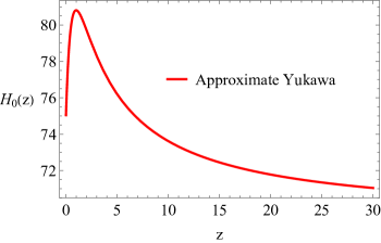
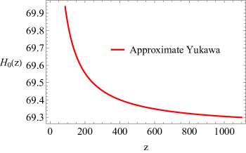
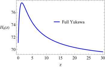
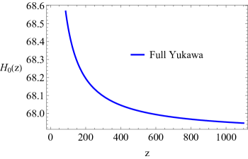
Figure 1: Plot of $H_{0}(z)$ as a function of $z$. We have used the integral (35) for the approximated/full Yukawa models in the low/high redshift interval. We have used the best-fit values from Table 1.

Put differently, Eq. (35) indicates that the Hubble constant’s value is contingent on the particular measurement associated with a redshift $z$. This equation was obtained from Eq. (34), which is also known as the look-back time and was studied recently in Capozziello et al. (2023) concerning its’ possible role on the Hubble tension. In the present paper, we argued that the look-back time quantity can be interpreted as the uncertainty in time by Eq. (30) when applied to the massive graviton. The current work also demonstrates the inherent emergence of this equation within the framework of Yukawa cosmology.

In Fig. 1, we plot $H_{0}(z)$ as a function of the redshift $z$. Initially, the Hubble constant increases with the increase of $z$; however, at a specific redshift, there is a turning point after which the Hubble constant decreases with increasing $z$. As evident from Eq. (34), there exists an inverse relationship between the uncertainty in time and the value of the Hubble constant

$$\Delta t\sim\frac{z\,t_{0}}{1+z}\sim\frac{k}{H_{0}},$$ (36)

or, if we use Eq. (29) we can write alternatively,

$$\Delta t\sim\frac{\Delta x}{c}\sim\frac{k}{H_{0}}.$$ (37)

where $k$ is some factor of proportionality. For exceedingly large redshift values, such as those associated with the Cosmic Microwave Background Radiation, we encounter a scenario with greater uncertainty in time and less uncertainty in the graviton mass. Given that the uncertainty in time is inversely proportional to the Hubble constant, this results in a situation where we get a smaller value for the Hubble constant. That agrees with the $H_{0}=67.4\pm 0.5$ km/s/Mpc value reported in Aghanim et al. (2020). Conversely, for smaller redshift values or local measurements, as observed in cases in galactic scales or cases like Cepheids and Supernovae Type Ia (SNe Ia), there is reduced uncertainty in time, leading to heightened uncertainty in the graviton mass. Consequently, this effect results in a higher value for the Hubble constant. That also agrees with the $H_{0}=73.04\pm 1.04$ km/s/Mpc value reported in Riess et al. (2022).

Rewriting Eq. (37) in terms of $\lambda$ and differentiating it,

$$\lambda(z)\sim\frac{c\,k}{H_{0}(z)}\Longrightarrow d\lambda=c\,k\Bigg{|}\frac{dH_{0}}{H_{0}^{2}}\Bigg{|}.$$ (38)

One can also get a relation between the uncertainty in the graviton’s mass and the uncertainty in the Hubble constant given by

$$\Delta\lambda=\frac{c\,k}{H_{0}}\Bigg{|}\frac{\Delta H_{0}}{H_{0}}\Bigg{|}=\lambda\Bigg{|}\frac{\Delta H_{0}}{H_{0}}\Bigg{|},$$ (39)

where $d\lambda\simeq\Delta\lambda$, and $dH_{0}\simeq\Delta H_{0}$. Since $\lambda=\hbar/(m_{g}c)$, we can finally write

$$\Bigg{|}\frac{\Delta\lambda}{\lambda}\Bigg{|}\sim\Bigg{|}\frac{\Delta m_{g}}{m_{g}}\Bigg{|}\sim\Bigg{|}\frac{\Delta H_{0}}{H_{0}}\Bigg{|}.$$ (40)

A similar result was obtained for the case of massive photons in Capozziello et al. (2020a). In the present paper, we argued that this intricacy in the Hubble constant can thus be explained through the lens of fundamental limitations stemming from the uncertainty relation when applied to the graviton. The measurement of the Hubble constant is intricately tied to length scales and is intricately linked to the uncertainty in time. Hence, the challenges associated with the Hubble constant find their roots in these fundamental limitations dictated by the uncertainty relation in the context of graviton measurements. According to (38), we can also say that the uncertainty in the graviton mass is proportional to the uncertainty in the Hubble constant.

V Discussions and observational constraints

V.1 Type Ia supernovae data

We will be examining the SNe Ia data through the Pantheon+ sample (Brout et al., 2022), an enhanced version succeeding the original Pantheon sample (Scolnic et al., 2018). This dataset comprises 1701 data points within the redshift range of $0.001\leq z\leq 2.26$. The merit function can be briefly formulated in matrix notation to facilitate our analysis, denoted by bold symbols, as:

$$\chi_{\text{SNe}}^{2}=\mathbf{\Delta D}(z,\theta,M)^{\dagger}\mathbf{C}^{-1}\mathbf{\Delta D}(z,\theta,M),$$ (41)

where $[\mathbf{\Delta D}(z,\theta,M)]_{i}=m_{B,i}-M-\mu_{th}(z_{i},\theta)$ and $\mathbf{C}=\mathbf{C}_{\text{stat}}+\mathbf{C}_{\text{sys}}$ is the total uncertainty covariance matrix, where the matrices $\textbf{C}_{\text{stat}}$ and $\textbf{C}_{\text{sys}}$ accounts for the statistical and systematic uncertainties, respectively. In this equation, $\mu_{i}=m_{B,i}-M$ represents the observational distance modulus for the Pantheon+ sample. This value is derived using a modified version of Tripp’s formula (Tripp, 1998), incorporating three nuisance parameters calibrated to zero through the BBC (BEAMS with Bias Corrections) approach (Kessler and Scolnic, 2017). Consequently, the Pantheon+ sample provides the corrected apparent B-band magnitude $m_{B,i}$ directly for a fiducial SNe Ia at redshift $z_{i}$, with $M$ representing the fiducial magnitude of an SNe Ia. The estimation of $M$ must be performed jointly with the model’s free parameters under investigation.

The theoretical distance modulus for a spatially flat FLRW spacetime is given by:

$$\mu_{th}(z_{i},\theta)=5\log_{10}{\left[\frac{d_{L}(z_{i},\theta)}{\text{Mpc}}\right]}+25,$$ (42)

with $d_{L}(z_{i},\theta)$ the luminosity distance given by

$$d_{L}(z_{i},\theta)=c(1+z_{i})\int_{0}^{z_{i}}{\frac{dz^{\prime}}{H_{th}(z^{\prime},\theta)}}.$$ (43)

Here, $c$ denotes the speed of light, measured in units of km/s. It is noteworthy that the luminosity distance is contingent on the theoretical Hubble parameter, defined by Eq. (III.1) in the context of Yukawa cosmology and Eq. (24) for the $\Lambda$CDM model. Consequently, the only additional free parameter introduced is the nuisance parameter $M$, for which we adopt the prior range $-20<M<-18$ in our MCMC analysis.

Like the Pantheon sample, a degeneracy exists between the nuisance parameter $M$ and $H_{0}$. To effectively constrain the free parameter $H_{0}$ solely through SNe Ia data, it becomes imperative to incorporate the SH0ES (Supernovae and $H_{0}$ for the Equation of State of dark energy program) Cepheid host distance anchors, as follows:

$$\chi^{2}_{\text{Cepheid}}=\Delta\textbf{D}_{\text{Cepheid}}\left(M\right)^{\dagger}\textbf{C}^{-1}\Delta\textbf{D}_{\text{ Cepheid}}\left(M\right),$$ (44)

where $\left[\Delta\textbf{D}_{\text{Cepheid}}\left(M\right)\right]_{i}=\mu_{i}\left(M\right)-\mu_{i}^{\text{Cepheid}}$, with $\mu_{i}^{\text{Cepheid}}$ the Cepheid calibrated host-galaxy distance obtained by SH0ES (Riess et al., 2022). Therefore, in establishing the correspondence, Cepheid distances are utilized as the “theory” instead of employing the model under study to calibrate $M$. This approach accounts for the sensitivity of the difference $\mu_{i}\left(M\right)-\mu_{i}^{\text{Cepheid}}$ to both $M$ and $H_{0}$ while being relatively insensitive to other parameters like $\Omega_{m,0}$. In this context, the Pantheon+ sample supplies $\mu_{i}^{\text{Cepheid}}$, with the total uncertainty covariance matrix for Cepheid encapsulated within the overall uncertainty covariance matrix $\mathbf{C}$. Consequently, we can formulate the merit function for the SNe Ia data as follows:

$$\chi_{\text{SNe}}^{2}=\mathbf{\Delta D^{\prime}}(z,\theta,M)^{\dagger}\mathbf{C}^{-1}\mathbf{\Delta D^{\prime}}(z,\theta,M),$$ (45)

where

$$\Delta\mathbf{D^{\prime}}_{i}=\left\{\begin{array}[]{ll}m_{B,i}-M-\mu_{i}^{\text{Cepheid}}&i\in\text{Cepheid host}\\ \\ m_{B,i}-M-\mu_{th}(z_{i},\theta)&\text{otherwise}\end{array}\right..$$ (46)

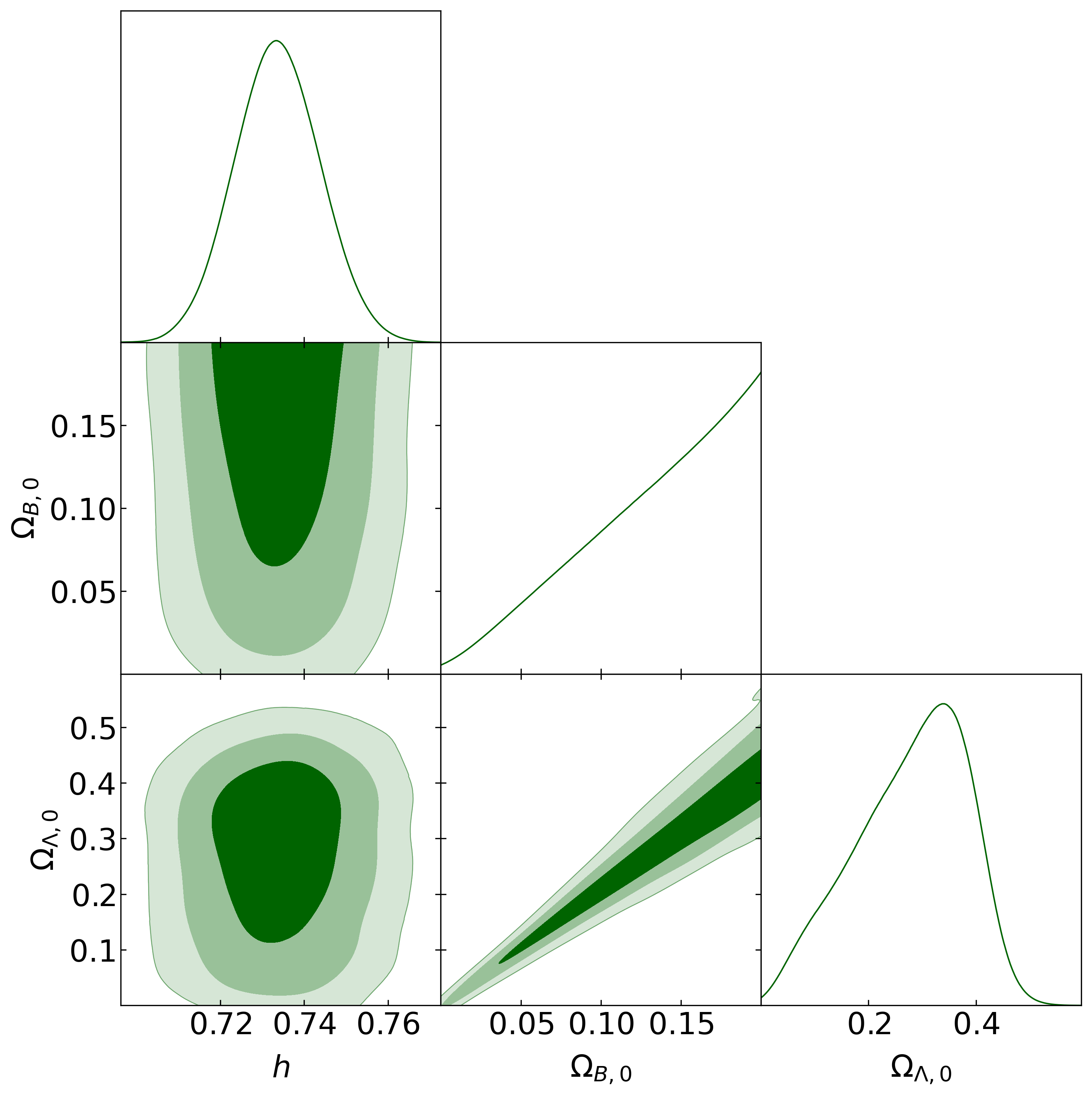
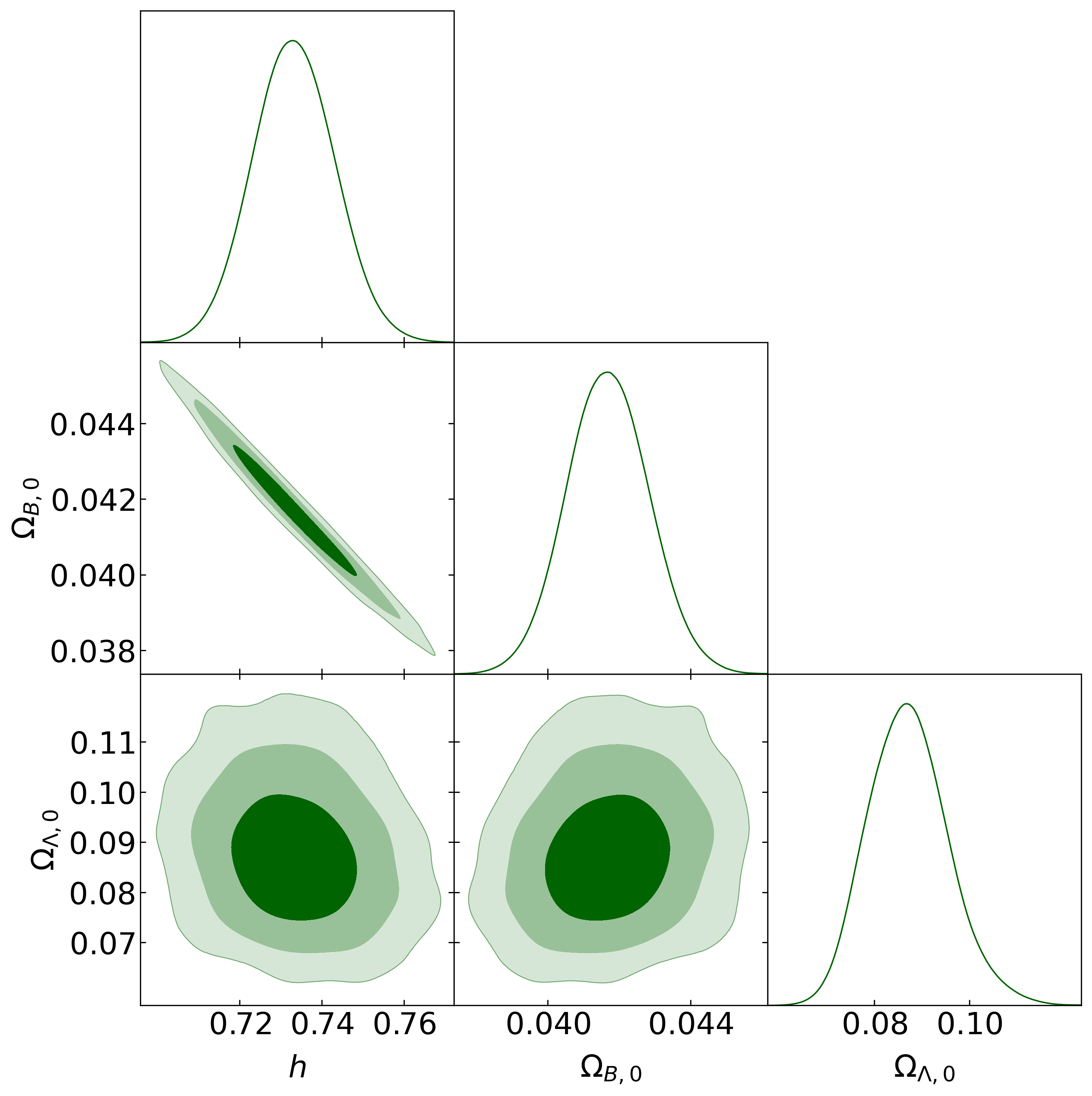
Figure 2: Posterior distribution and joint marginalized regions of the free parameters space of the full Yukawa model, obtained by the MCMC analysis and SNe Ia data (left panel) and SNe Ia data using CMB Gaussian prior (right panel). The admissible joint regions correspond to $1\sigma$, $2\sigma$, and $3\sigma$ CL, respectively.

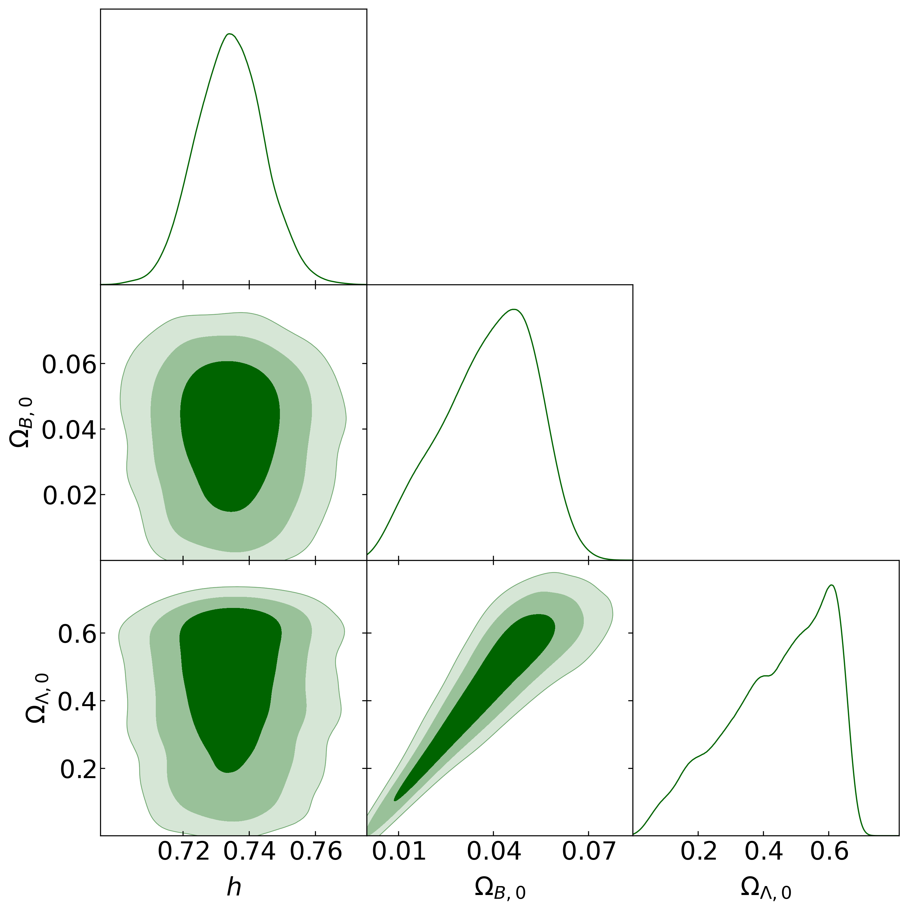
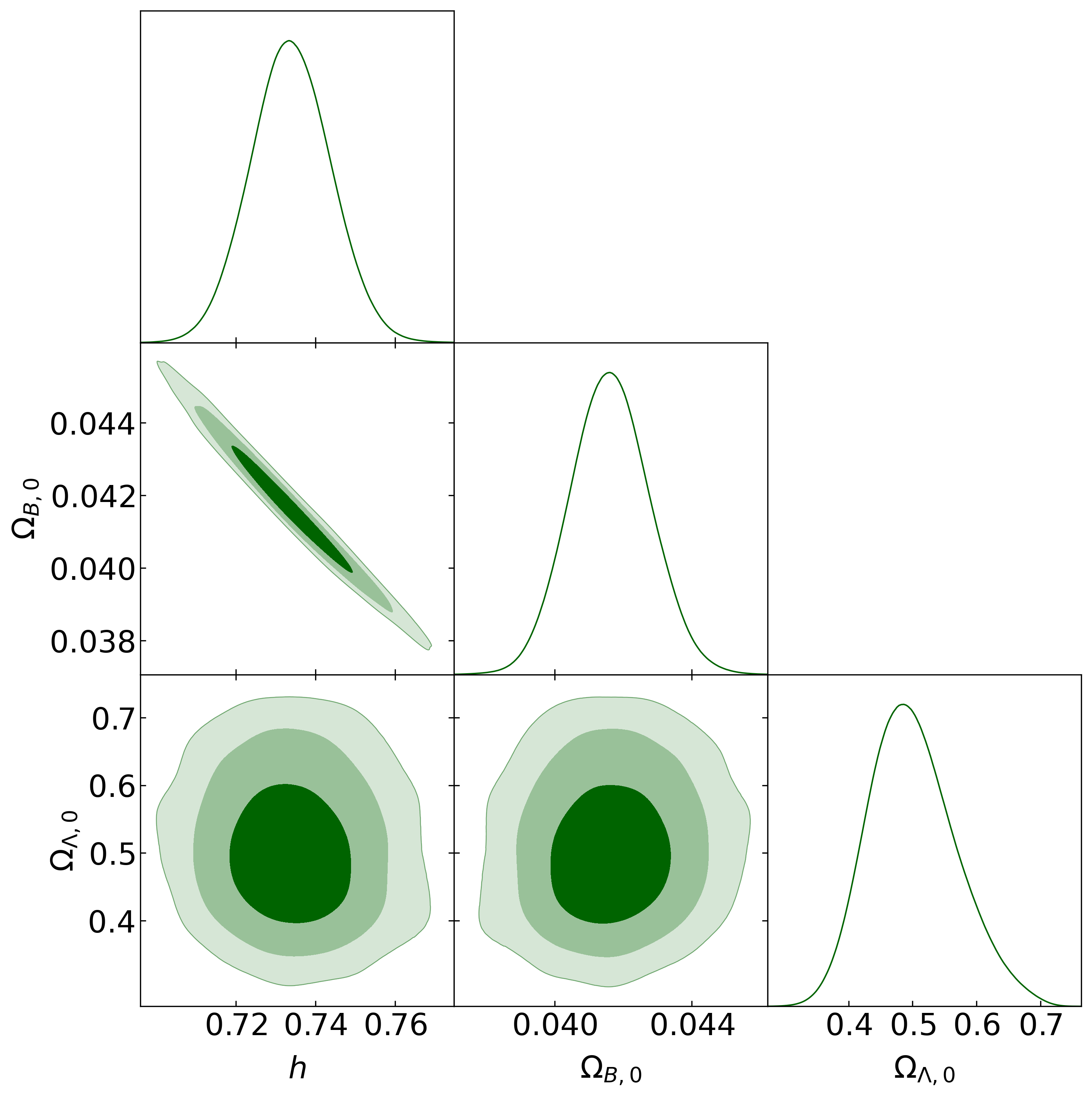
Figure 3: Posterior distribution and joint marginalized regions of the free parameters space of the approximated Yukawa model, obtained by the MCMC analysis and SNe Ia data (left panel) and SNe Ia data using Gaussian priors (right panel). The admissible joint regions correspond to $1\sigma$, $2\sigma$, and $3\sigma$ CL, respectively.

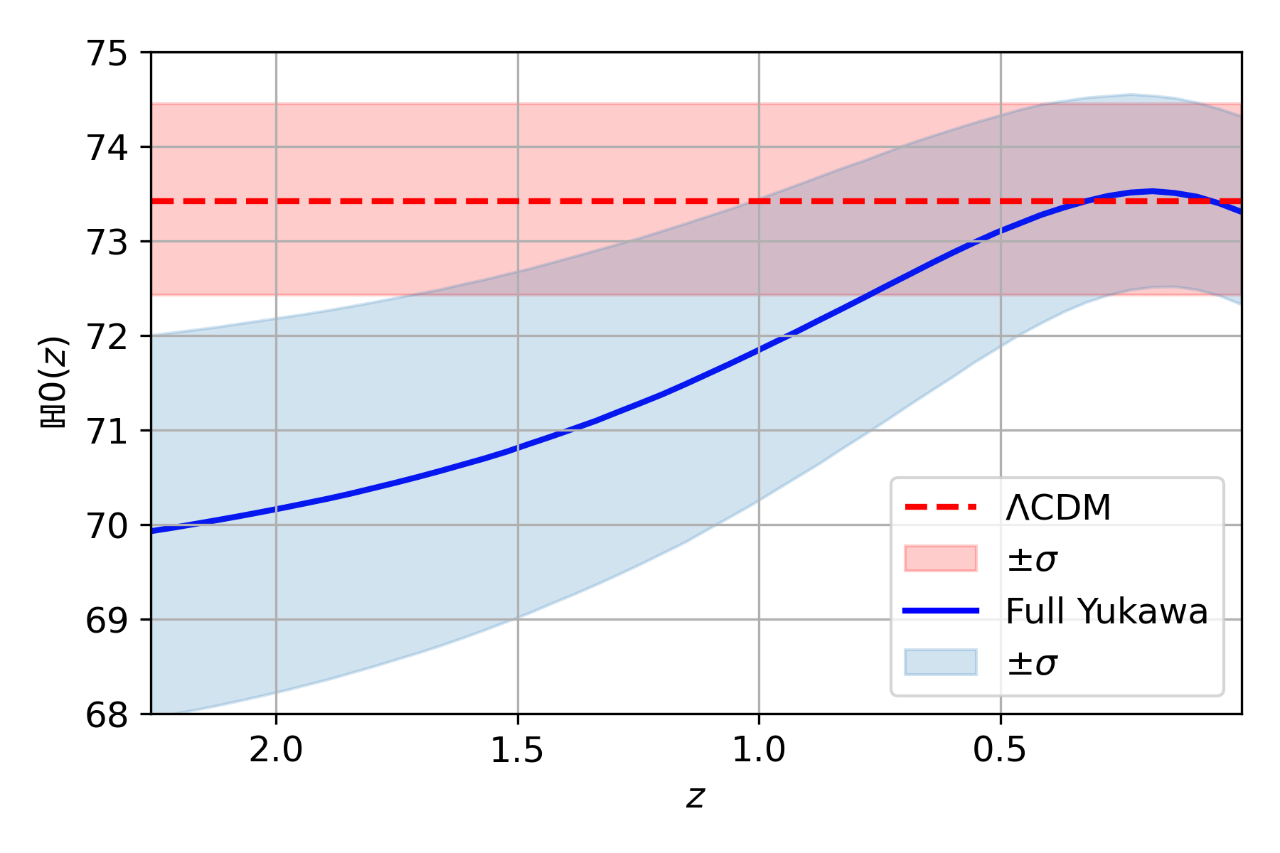
Figure 4: Left panel: $\mathbb{H}_{0}$ diagnostic for full Yukawa solution using SNe Ia data. Right panel: $\mathbb{H}_{0}$ diagnostic for full Yukawa solution using SNe Ia data with Gaussian prior.

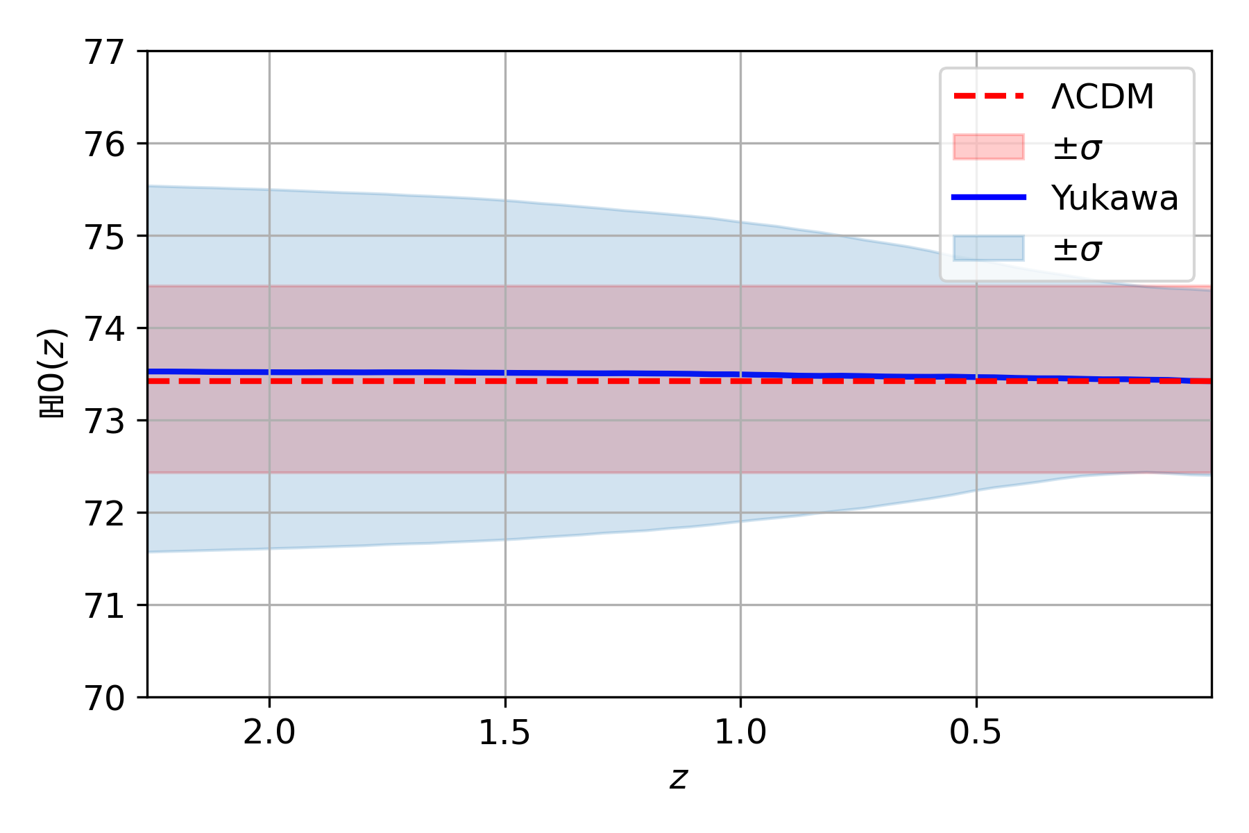
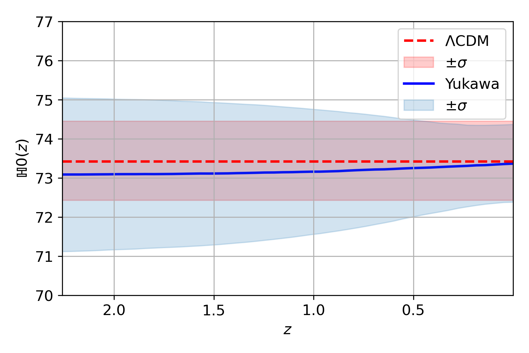
Figure 5: Left panel: $\mathbb{H}_{0}$ diagnostic for approximated Yukawa solution using SNe Ia data. Right panel: $\mathbb{H}_{0}$ diagnosis for the approximated Yukawa solution using SNe Ia data and Gaussian prior.

It is crucial to note that moving forward, we will exclude the consideration of the free parameter $M$ and concentrate solely on the analysis of the free parameters specific to each model. Additionally, since the best-fit parameters minimize the merit function, $\chi_{\text{min}}^{2}$, we can utilize the evaluation of these best-fit parameters as an indicator of the goodness of the fit: a smaller value of $\chi_{\text{min}}^{2}$ corresponds to a better fit.

Parameter	Approximated Yukawa	Full Yukawa
$h$	$\left\{\begin{array}[]{cc}0.734\pm 0.010&\text{Flat priors}\\ 0.734\pm 0.010&\text{Gaussian priors}\end{array}\right.$	$\left\{\begin{array}[]{cc}0.735\pm 0.010&\text{Flat priors}\\ 0.733\pm 0.010&\text{Gaussian priors}\end{array}\right.$
$\Omega_{B,0}$	$\left\{\begin{array}[]{cc}0.040^{+0.013}_{-0.017}&\text{Flat priors}\\ 0.041^{+0.001}_{-0.001}&\text{Gaussian priors}\end{array}\right.$	$\left\{\begin{array}[]{cc}0.141^{+0.06}_{-0.04}&\text{Flat priors}\\ 0.042^{+0.001}_{-0.001}&\text{Gaussian priors}\end{array}\right.$
$\Omega_{\Lambda,0}$	$\left\{\begin{array}[]{cc}0.471^{+0.137}_{-0.208}&\text{Flat priors}\\ 0.49^{+0.1}_{-0.1}&\text{Gaussian priors}\end{array}\right.$	$\left\{\begin{array}[]{cc}0.292^{+0.09}_{-0.12}&\text{Flat priors}\\ 0.087^{+0.008}_{-0.008}&\text{Gaussian priors}\end{array}\right.$
$\alpha$	$\left\{\begin{array}[]{cc}0.41^{+1.08}_{-0.32}&\text{Flat priors}\\ 0.35^{+0.15}_{-0.14}&\text{Gaussian priors}\end{array}\right.$	$\left\{\begin{array}[]{cc}1.09^{+1.62}_{-0.48}&\text{Flat priors}\\ 6.07^{+0.47}_{-0.44}&\text{Gaussian priors}\end{array}\right.$
$\lambda$ [Mpc]	$\left\{\begin{array}[]{cc}2707.43^{+1165.18}_{-1289.92}&\text{Flat priors}\\ 2543.95^{+384.48}_{-513.62}&\text{Gaussian priors}\end{array}\right.$	$\left\{\begin{array}[]{cc}3772.27^{+704.96}_{-582.22}&\text{Flat priors}\\ 4833.84^{+121.30}_{-129.29}&\text{Gaussian priors}\end{array}\right.$
$\chi_{\text{min}}^{2}$	$\left\{\begin{array}[]{cc}1523.0&\text{Flat priors}\\ 1523.0&\text{Gaussian priors}\end{array}\right.$	$\left\{\begin{array}[]{cc}1522.50&\text{Flat priors}\\ 1522.51&\text{Gaussian priors}\end{array}\right.$

Table 1: Best-fit values for the approximated Yukawa cosmology and full Yukawa cosmology with uniform and Gaussian priors. The values were obtained by the MCMC analysis using SNe Ia data, and the uncertainties correspond to $1\sigma$ CL. Note here that the Hubble constant is $H_{0}=100\,h$ km/s/Mpc.

V.2 Discussions

We analyzed the full Yukawa and the approximated Yukawa models using SNe Ia data in Figs. 2 and 3, we depict the posterior distribution and joint marginalized regions of the free parameters space generated from the MCMC analysis utilizing SNe Ia data with and without Gaussian priors for both the full Yukawa and approximated Yukawa models. Table 1 present our results for the best-fit values for the cosmological models and Yukawa parameters. It can be seen that there is no best fit obtained for $\Omega_{B,0}$ in the full Yukawa model with SNe Ia data, whereas a robust constraint is achieved for the approximated Yukawa model. In the approximated model, the constraint on $\Omega_{B,0}$ is exclusively derived from SNe Ia data due to the relationship between $\Omega_{DM,0}$ and $\Omega_{B,0}$, effectively breaking the degeneracy between these two parameters. Additionally, the plots reveal a difference when Gaussian priors are employed, leading to improved constraints on the parameters, including the Yukawa parameters. However, the values of $\chi_{min}^{2}$ remain very similar. On the contrary, Figs. 4 and 5 display plots for the $\mathbb{H}_{0}$ diagnostic for both the approximated and full Yukawa solutions using Eq. (28). The $\mathbb{H}_{0}$ diagnostic indicates that the dynamical value of the Hubble constant tends to be lower than $70$ km/sh/Mpc at high redshifts, potentially suggesting a alleviation of the Hubble tension. Notably, the running Hubble constant only alleviates the Hubble tension for local and large redshift values in the case of the full Yukawa model, unlike the approximated Yukawa model, which is effectively very similar to the $\Lambda$CDM model, as evident from the plot. Therefore, this approach does not yield a satisfactory result for either model.

To address this inconsistency, we will explore further in more detail the role of uncertainty relations on the Hubble tension. As we pointed out, the Hubble tension arises from a discrepancy in the measurements of the Hubble constant $H_{0}$, based on observations of objects in our local Universe (Cepheid variable stars and Type Ia supernovae) and the measurements based on the CMB radiation. As argued in the present paper, this tension might result from the measurements performed on different scales. Based on this, we showed that the following relation should hold:

$$\Bigg{|}\frac{\Delta\lambda}{\lambda^{\rm CMB}}\Bigg{|}\sim\Bigg{|}\frac{\Delta m_{g}}{m_{g}^{\rm CMB}}\Bigg{|}\sim\Bigg{|}\frac{\Delta H_{0}}{H_{0}^{\rm CMB}}\Bigg{|},$$ (47)

where

$$\Delta\lambda = \lambda^{\rm CMB}-\lambda^{\rm SNeIa},$$ (48)

$$\Delta m_{g} = m_{g}^{\rm CMB}-m_{g}^{\rm SNeIa},$$ (49)

$$\Delta H_{0} = H_{0}^{\rm CMB}-H_{0}^{\rm SNeIa}.$$ (50)

Based on our analysis of the SNe Ia data, we have demonstrated that the Yukawa cosmology’s Hubble constant aligns with the Hubble constant value in the $\Lambda\text{CDM}$ model. This convergence is detailed in Table 1. Namely, we obtained for the Hubble constant $H_{0}^{\rm SNeIa}\sim 73.4$ km/s/Mpc. This alignment between the Hubble constant values in Yukawa cosmology and the $\Lambda\text{CDM}$ model, as demonstrated in our analysis of SNe Ia data, prompts us to extend this expectation to the analysis of CMB data. We anticipate this agreement will persist, providing further coherence between the two models. From a theoretical point of view, this fact is shown in Fig. 1. One can see for both models that for high redshift ($z\sim 1000)$, we indeed get a value for the Hubble constant that is consistent with Aghanim et al. (2020). Namely, let us take the value $H_{0}^{\rm CMB}=67.40\pm 0.5$ km/s/Mpc obtained from Aghanim et al. (2020), to get

$$\Bigg{|}\frac{\Delta H_{0}}{H_{0}^{\rm CMB}}\Bigg{|}\sim 0.089.$$ (51)

Now, since we showed that according to Eqs. (32) and (33), there exists a relation between the Hubble constant and wavelength; one can compute:

$$\lambda^{\rm CMB}\sim\frac{c\,k^{\rm CMB}}{H_{0}^{\rm CMB}}\sim 4451\,k^{\rm CMB}{\rm Mpc},$$ (52)

where can set $k^{\rm CMB}\sim 1$ and, we also have,

$$\lambda^{\rm SNeIa}\sim\frac{c\,k^{\rm SNeIa}}{H_{0}^{\rm SNeIa}}\sim 4087\,k^{\rm SNeIa}{\rm Mpc}.$$ (53)

In this way we get

$$\Bigg{|}\frac{\Delta\lambda}{\lambda^{\rm CMB}}\Bigg{|}\sim 0.082.$$ (54)

Therefore, an excellent agreement exists with the result (51). Let us, however, comment briefly on the fact that from observational constraints given in Table 1, we see that we got four values for $\lambda$ and, although all these are of Mpc order and close to the value $4087$ Mpc, they are not the same. That has to do with the fact that we have chains of data/measurements. Hence we can take as an effective value for $\lambda_{\rm eff}$ the average value, which is close to $\lambda_{\rm eff}\sim 3464.4$ Mpc. Comparing it with the equation (53), we get $k^{\rm SNeIa}\sim 0.85$. On the other hand, for CMB, the value of $k^{\rm CMB}$ might not be exactly one as we approximated it, but close to one, say $k^{\rm CMB}\sim k^{\rm SNeIa}$, and, again, the final result will not change much and can be close to (51). However, more work is needed to obtain better constraints for $\lambda$. One can also compute the corresponding mass for the graviton, but first let us see from (IV.2) that for $\lambda^{\rm CMB}=\Delta x^{\rm CMB}$ we have more uncertainty in position but more precision on the momentum,

$$\Delta p^{\rm CMB}\sim\frac{\hbar}{\Delta x^{\rm CMB}}\sim 7.69\times 10^{-61}\rm{N\,s},$$ (55)

compared to the case the case for $\lambda^{\rm SNeIa}=\Delta x^{\rm SNeIa}$ where we have less uncertainty in position but more uncertainty on the momentum,

$$\Delta p^{\rm SNeIa}\sim\frac{\hbar}{\Delta x^{\rm SNeIa}}\sim 8.33\times 10^{-61}\rm{N\,s}.$$ (56)

We can further compute also the mass for each case

$$m^{\rm CMB}\sim\frac{\hbar}{\lambda^{\rm CMB}c}\sim 2.56\times 10^{-69}{\rm kg},$$ (57)

and

$$m^{\rm SNeIa}\sim\frac{\hbar}{\lambda^{\rm SNeIa}c}\sim 2.79\times 10^{-69}{\rm kg}.$$ (58)

Finally, if we use (47) we get

$$\Bigg{|}\frac{\Delta m}{m^{\rm CMB}}\Bigg{|}\sim 0.089.$$ (59)

Again, as was expected, this result is in excellent agreement with Eq. (51). The Hubble tension, therefore, might be explained by the fundamental quantum mechanical limitations of the measurements in cosmology. The relation between $\lambda$ and $H_{0}$ should be, in principle, universal and should hold for any measurement to add some values for $H_{0}$ from different measurements. Let us finally point out that the energy density of dark energy also depends on $\lambda$, and this implies

$$\rho^{\rm SNeIa}_{\Lambda}\sim\frac{3\,\alpha\,c^{2}}{8\pi G\lambda_{\rm SNeIa}^{2}},$$ (60)

which also implies fundamental quantum mechanical limitations in measuring $\rho_{\Lambda}$. On the other hand, from the relation $\lambda^{\rm SNeIa}\sim c\,k^{\rm SNeIa}/H_{0}^{\rm SNeIa}$ for the dark energy density parameter we get $\Omega_{\Lambda,0}^{\Lambda\text{CDM}}\sim\alpha/[k^{2}_{\rm SNeIa}(1+\alpha)]$.

VI Conclusions

In the present paper, we used the Yukawa modified gravity, which has two parameters, $\alpha$ and $\lambda$, related to the graviton mass, to address the Hubble tension. In particular, we used two models: full and approximated Yukawa models. To address the Hubble tension, first, we used the $\mathbb{H}_{0}$ diagnostic Hubble constant, a showdown that it tends to be lower than $70$ km/sh/Mpc at high redshifts, suggesting a possible alleviation of the Hubble tension. However, the running Hubble constant only tends to alleviate the Hubble tension in the case of the full Yukawa model, unlike the approximated Yukawa model, which is effectively very similar to the $\Lambda$CDM model, indicating that the resolution of the Hubble tension could be more attainable through our approach.

This paper primarily focuses on investigating the impact of uncertainty relations on the phenomenon of the Hubble tension, constituting its main result. Since dark matter and dark energy are related to each other in terms of gravitons’ wavelength $\lambda$, it is natural to apply the uncertainty relations to the graviton where $\lambda$ is defined as $\lambda=\hbar/(m_{g}c)$. In doing so, we have obtained the energy-time uncertainty relation, which shows that the uncertainty in time exhibits an inverse correlation with the value of the Hubble constant, meaning that the measurement of the Hubble constant is intricately tied to length scales and is intricately linked to the uncertainty in time. Thought the MCMC analyses using the SNe Ia data we showed that the Hubble constant in Yukawa cosmology is the same as in $\Lambda$CDM. In general, this is expected to be the case for CMB data. As we have argued in the present paper, to resolve this inconsistency, in cosmological scales, it was found that the uncertainty in time coincides with the look-back time quantity. Therefore, the Hubble constant, in general, depends on the measurements of the length scale with a given redshift. This indicates that when there is increased uncertainty in time, especially for measurements with a high redshift value (such as the CMB), we have a smaller value for the Hubble constant. Similarly, if there is less uncertainty in time, the case for local measurements with a smaller redshift value (such as the Cepheids and SNe Ia) implies a higher value for the Hubble constant. These results show that the Hubble tension arises due to fundamental limitations inherent in cosmology measurements of the graviton’s wavelength (scales) by the uncertainty relation.

CRediT authorship contribution statement

Kimet Jusufi: Conceptualization, Methodology, Formal analysis, Investigation, Writing – original draft, Writing – review & editing, Supervision. Esteban González: Conceptualization, Methodology, Software, Visualization, Validation, Formal analysis, Investigation, Writing – review & editing, Funding acquisition, Supervision, Project administration. Genly Leon: Conceptualization, Writing – review & editing, Investigation, Funding acquisition, Project administration.

Declaration of competing interest

The authors declare that they have no known competing financial interests or personal relationships that could have appeared to influence the work reported in this paper.

Data Availability

Section V cited the data underlying this article.

References

- Vagnozzi (2023) S. Vagnozzi, Universe 9, 393 (2023), arXiv:2308.16628 [astro-ph.CO] .
- Vagnozzi (2020) S. Vagnozzi, Phys. Rev. D 102, 023518 (2020), arXiv:1907.07569 [astro-ph.CO] .
- Di Valentino et al. (2020) E. Di Valentino, A. Melchiorri, O. Mena, and S. Vagnozzi, Phys. Dark Univ. 30, 100666 (2020), arXiv:1908.04281 [astro-ph.CO] .
- Riess et al. (2022) A. G. Riess et al., Astrophys. J. Lett. 934, L7 (2022), arXiv:2112.04510 [astro-ph.CO] .
- Aghanim et al. (2020) N. Aghanim et al. (Planck), Astron. Astrophys. 641, A6 (2020), [Erratum: Astron.Astrophys. 652, C4 (2021)], arXiv:1807.06209 [astro-ph.CO] .
- Peebles (1984) P. J. E. Peebles, Astrophys. J. 277, 470 (1984).
- Bond and Efstathiou (1984) J. R. Bond and G. Efstathiou, Astrophys. J. Lett. 285, L45 (1984).
- Trimble (1987) V. Trimble, Ann. Rev. Astron. Astrophys. 25, 425 (1987).
- Turner (1991) M. S. Turner, in UCLA International Conference on Trends in Astroparticle Physics (1991) pp. 3–42.
- Salucci et al. (2021) P. Salucci et al., Front. in Phys. 8, 603190 (2021), arXiv:2011.09278 [gr-qc] .
- Carroll et al. (1992) S. M. Carroll, W. H. Press, and E. L. Turner, Ann. Rev. Astron. Astrophys. 30, 499 (1992).
- Perlmutter et al. (1998) S. Perlmutter et al. (Supernova Cosmology Project), Nature 391, 51 (1998), arXiv:astro-ph/9712212 .
- Riess et al. (1998) A. G. Riess et al. (Supernova Search Team), Astron. J. 116, 1009 (1998), arXiv:astro-ph/9805201 .
- Peebles and Ratra (2003) P. J. E. Peebles and B. Ratra, Rev. Mod. Phys. 75, 559 (2003), arXiv:astro-ph/0207347 .
- Weinberg (1989) S. Weinberg, Rev. Mod. Phys. 61, 1 (1989).
- Zlatev et al. (1999) I. Zlatev, L.-M. Wang, and P. J. Steinhardt, Phys. Rev. Lett. 82, 896 (1999), arXiv:astro-ph/9807002 .
- Padmanabhan (2003) T. Padmanabhan, Phys. Rept. 380, 235 (2003), arXiv:hep-th/0212290 .
- Starobinsky (1980) A. A. Starobinsky, Phys. Lett. B 91, 99 (1980).
- Guth (1981) A. H. Guth, Phys. Rev. D 23, 347 (1981).
- D’Agostino and Luongo (2022) R. D’Agostino and O. Luongo, Phys. Lett. B 829, 137070 (2022), arXiv:2112.12816 [astro-ph.CO] .
- D’Agostino et al. (2022) R. D’Agostino, O. Luongo, and M. Muccino, Class. Quant. Grav. 39, 195014 (2022), arXiv:2204.02190 [gr-qc] .
- Capozziello and Shokri (2022) S. Capozziello and M. Shokri, Phys. Dark Univ. 37, 101113 (2022), arXiv:2209.06670 [gr-qc] .
- Di Valentino et al. (2021) E. Di Valentino et al., Astropart. Phys. 131, 102605 (2021), arXiv:2008.11284 [astro-ph.CO] .
- Perivolaropoulos and Skara (2022) L. Perivolaropoulos and F. Skara, New Astron. Rev. 95, 101659 (2022), arXiv:2105.05208 [astro-ph.CO] .
- D’Agostino and Nunes (2023) R. D’Agostino and R. C. Nunes, Phys. Rev. D 108, 023523 (2023), arXiv:2307.13464 [astro-ph.CO] .
- Capozziello et al. (2007) S. Capozziello, A. Stabile, and A. Troisi, Phys. Rev. D 76, 104019 (2007), arXiv:0708.0723 [gr-qc] .
- Capozziello et al. (2015) S. Capozziello, G. Lambiase, M. Sakellariadou, and A. Stabile, Phys. Rev. D 91, 044012 (2015), arXiv:1410.8316 [gr-qc] .
- De Martino and De Laurentis (2017) I. De Martino and M. De Laurentis, Phys. Lett. B 770, 440 (2017), arXiv:1705.02366 [astro-ph.CO] .
- Benisty and Capozziello (2023) D. Benisty and S. Capozziello, Phys. Dark Univ. 39, 101175 (2023), arXiv:2301.06614 [astro-ph.GA] .
- Jusufi et al. (2023a) K. Jusufi, G. Leon, and A. D. Millano, Phys. Dark Univ. 42, 101318 (2023a), arXiv:2304.11492 [gr-qc] .
- González et al. (2023) E. González, K. Jusufi, G. Leon, and E. N. Saridakis, Phys. Dark Univ. 42, 101304 (2023), arXiv:2305.14305 [astro-ph.CO] .
- Jusufi and Sheykhi (2024) K. Jusufi and A. Sheykhi, (2024), arXiv:2402.00785 [gr-qc] .
- Jusufi et al. (2023b) K. Jusufi, A. Sheykhi, and S. Capozziello, Phys. Dark Univ. 42, 101270 (2023b), arXiv:2303.14127 [gr-qc] .
- Capozziello and De Laurentis (2011) S. Capozziello and M. De Laurentis, Phys. Rept. 509, 167 (2011), arXiv:1108.6266 [gr-qc] .
- Capozziello et al. (2020a) S. Capozziello, M. Benetti, and A. D. A. M. Spallicci, Found. Phys. 50, 893 (2020a), arXiv:2007.00462 [gr-qc] .
- Spallicci et al. (2022) A. D. A. M. Spallicci, M. Benetti, and S. Capozziello, Foundations of Physics 52 (2022), 10.1007/s10701-021-00531-z.
- Trivedi (2023) O. Trivedi, Phys. Dark Univ. 39, 101150 (2023), arXiv:2207.10570 [gr-qc] .
- Capozziello (2002) S. Capozziello, Int. J. Mod. Phys. D 11, 483 (2002), arXiv:gr-qc/0201033 .
- Sotiriou and Faraoni (2010) T. P. Sotiriou and V. Faraoni, Rev. Mod. Phys. 82, 451 (2010), arXiv:0805.1726 [gr-qc] .
- De Felice and Tsujikawa (2010) A. De Felice and S. Tsujikawa, Living Rev. Rel. 13, 3 (2010), arXiv:1002.4928 [gr-qc] .
- Capozziello et al. (2020b) S. Capozziello, V. B. Jovanović, D. Borka, and P. Jovanović, Phys. Dark Univ. 29, 100573 (2020b), arXiv:2004.11557 [gr-qc] .
- Capozziello et al. (2008) S. Capozziello, A. Stabile, and A. Troisi, Class. Quant. Grav. 25, 085004 (2008), arXiv:0709.0891 [gr-qc] .
- Capozziello et al. (2009) S. Capozziello, A. Stabile, and A. Troisi, Mod. Phys. Lett. A 24, 659 (2009), arXiv:0901.0448 [gr-qc] .
- Napolitano et al. (2012) N. R. Napolitano, S. Capozziello, A. J. Romanowsky, M. Capaccioli, and C. Tortora, Astrophys. J. 748, 87 (2012), arXiv:1201.3363 [astro-ph.CO] .
- De Martino et al. (2018) I. De Martino, R. Lazkoz, and M. De Laurentis, Phys. Rev. D 97, 104067 (2018), arXiv:1801.08135 [gr-qc] .
- Chae (2023a) K.-H. Chae, Astrophys. J. 952, 128 (2023a), [Erratum: Astrophys.J. 956, 69 (2023)], arXiv:2305.04613 [astro-ph.GA] .
- Chae (2023b) K.-H. Chae, (2023b), arXiv:2309.10404 [astro-ph.GA] .
- Hernandez (2023) X. Hernandez, Mon. Not. Roy. Astron. Soc. 525, 1401 (2023), arXiv:2304.07322 [astro-ph.GA] .
- Cardone and Capozziello (2011) V. F. Cardone and S. Capozziello, Mon. Not. Roy. Astron. Soc. 414, 1301 (2011), arXiv:1102.0916 [astro-ph.CO] .
- Krishnan et al. (2021) C. Krishnan, E. O. Colgáin, M. M. Sheikh-Jabbari, and T. Yang, Phys. Rev. D 103, 103509 (2021), arXiv:2011.02858 [astro-ph.CO] .
- Capozziello et al. (2023) S. Capozziello, G. Sarracino, and A. D. A. M. Spallicci, Phys. Dark Univ. 40, 101201 (2023), arXiv:2302.13671 [astro-ph.CO] .
- Brout et al. (2022) D. Brout et al., Astrophys. J. 938, 110 (2022), arXiv:2202.04077 [astro-ph.CO] .
- Scolnic et al. (2018) D. M. Scolnic et al. (Pan-STARRS1), Astrophys. J. 859, 101 (2018), arXiv:1710.00845 [astro-ph.CO] .
- Tripp (1998) R. Tripp, Astron. Astrophys. 331, 815 (1998).
- Kessler and Scolnic (2017) R. Kessler and D. Scolnic, Astrophys. J. 836, 56 (2017), arXiv:1610.04677 [astro-ph.CO] .