Quantum reversal: a general theory of coherent quantum absorbers

Abstract

The fascinating concept of coherent quantum absorber—which can absorb any photon emitted by another system while maintaining entanglement with that system—has found diverse implications in open quantum system theory and quantum metrology. This work generalizes the concept by proposing the so-called reversal conditions for the two systems, in which a “reverser” coherently reverses any effect of the other system on a field. The reversal conditions are rigorously boiled down to concise formulas involving the Petz recovery map and Kraus operators, thereby generalizing as well as streamlining the existing treatments of coherent absorbers.

1 Introduction

A coherent quantum absorber, as conceived by Stannigel et al. Stannigel et al. (2012), is a system that absorbs any photon emitted by another system while maintaining entanglement with that system. The idea has since found surprising implications, such as a technique for finding the steady states of open quantum systems Stannigel et al. (2012); Roberts and Clerk (2020); Roberts et al. (2021) and a method for constructing efficient continuous measurements for quantum parameter estimation Godley and Guta (2023); Yang et al. (2023). Remarkably, Yang, Huelga, and Plenio Yang et al. (2023) have recently shown that a method of measurement-backaction-noise cancellation Tsang and Caves (2010, 2012); Hammerer et al. (2009); Khalili and Polzik (2018)—which has seen significant experimental progress with atomic and optomechanical systems in recent years Møller et al. (2017); Junker et al. (2022); Jia et al. (2023)—can be regarded as a special case of coherent absorbers. This relation extends the potential impact of the absorber concept to the areas of magnetometry, optomechanics, and gravitational-wave detectors.

While the absorber concept is fascinating and promising, many special assumptions and a bewildering array of theoretical tools have been invoked to study it, such as quantum Markov semigroups, cascaded quantum networks Stannigel et al. (2012), matrix-product states Yang et al. (2023), and quantum detailed balance Roberts et al. (2021); Fagnola and Umanità (2010). The goal of this work is to tease out the essential ideas and make the absorber notion more rigorous as well as generalizable to other scenarios, far beyond the narrow setting of photon emission and absorption considered in prior works.

This generality calls for a different name for the generalized absorber conditions proposed here—I call them the reversal conditions. The key appeal of the reversal conditions is that they can be boiled down to concise formulas in terms of judiciously chosen concepts in open quantum system theory. Out go the quantum Markov semigroups, the matrix-product states, and many other extraneous concepts; in come antiunitary operators Parthasarathy (1992); Roberts et al. (2021), the Petz recovery map Petz (2010), and Kraus operators Holevo (2019) as the more fundamental ingredients of the reversal conditions.

This work is organized as follows. Sec. 2 introduces the basic model and defines the reversal condition. Sec. 3 discusses how a quantum detailed balance condition proposed by Fagnola and Umanità Fagnola and Umanità (2010) can simplify the reversal condition. Sec. 4 introduces a special reversal condition that eliminates an ambiguity in the general condition and may be more useful in experiment design. Theorem 2.1 and 4.1 are the key results that translate the conditions to the promised formulas.

2 The reversal condition

2.1 Model

Consider the model depicted by Fig. 1. Two systems, denoted as system A and B, are initially in a pure state $\ket{\psi}_{AB}$ in Hilbert space $\mathcal{H}_{A}\otimes\mathcal{H}_{B}$. A mode of a traveling field with initial state $\ket{\chi}_{E}$ in Hilbert space $\mathcal{H}_{E}$ interacts with system A according to a unitary operator $U$ on $\mathcal{H}_{A}\otimes H_{E}$. The field mode then evolves according to an intermediate unitary operator $U_{E}$ on $\mathcal{H}_{E}$, before interacting with system B according to a unitary operator $V$ on $\mathcal{H}_{B}\otimes\mathcal{H}_{E}$. A generalization of this model for interactions with multiple field modes will be discussed in Sec. 3. All Hilbert spaces are assumed to be finite-dimensional in the proofs for simplicity.

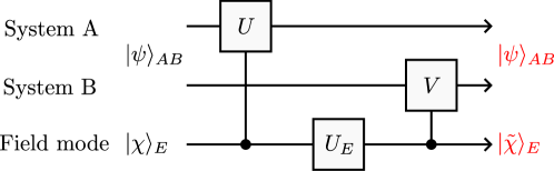
Figure 1: A quantum circuit illustrating the interactions between system A, system B, and the field mode.

Let $\mathcal{O}(\mathcal{H})$ be the set of operators on Hilbert space $\mathcal{H}$. An operator on operators is called a map in this work, also called a superoperator in the literature. After the unitary $U$, a channel for system A can be modeled by a completely positive, trace-preserving (CPTP) map $\mathcal{F}:\mathcal{O}(\mathcal{H}_{A})\to\mathcal{O}(\mathcal{H}_{A})$ given by

$$\mathcal{F}\rho_{A} \equiv\tr_{E}U(\rho_{A}\otimes\ket{\chi}_{E}\bra{\chi})U^{\dagger},$$ (1)

where $\rho_{A}$ is an arbitrary density operator on $\mathcal{H}_{A}$, $\tr_{xy\dots}$ is the partial trace with respect to $\mathcal{H}_{x}\otimes\mathcal{H}_{y}\otimes\dots$, and subscripts of $A$, $B$, and $E$ are used throughout this work to clarify the subspace to which each expression belongs. Suppose that a density operator $\sigma\in\mathcal{O}(\mathcal{H}_{A})$ is a steady state of $\mathcal{F}$, viz.,

$$\mathcal{F}\sigma =\sigma.$$ (2)

The spectral form of $\sigma$ is assumed to be

$$\sigma =\sum_{n}p_{n}\ket{n}_{A}\bra{n},$$ (3)

where $\{p_{n}:n=0,\dots,d_{A}-1\}$ are the eigenvalues of $\sigma$, $\{\ket{n}_{A}\in\mathcal{H}_{A}:n=0,1,\dots,d_{A}-1\}$ is an orthonormal basis of $\mathcal{H}_{A}$, $d_{x}$ is the dimension of $\mathcal{H}_{x}$, and each $\ket{n}_{A}$ is an eigenvector of $\sigma$ with eigenvalue $p_{n}$. $\sigma$ is assumed to be full-rank, viz., $p_{n}>0$ for all $n$.

Following Roberts et al. Roberts et al. (2021), assume that $d_{B}=d_{A}$ and $\ket{\psi}_{AB}$ is a purification of the steady state $\sigma$, given by

$$\ket{\psi}_{AB} =\sum_{n}\sqrt{p_{n}}\ket{n}_{A}\otimes\ket{\tilde{n}}_{B},$$ (4)

where

$$\ket{\tilde{n}}_{B} =W\theta\ket{n}_{A},$$ (5)

$W:\mathcal{H}_{A}\to\mathcal{H}_{B}$ is a unitary operator, and $\theta:\mathcal{H}_{A}\to\mathcal{H}_{A}$ is an antiunitary operator. The concept of antiunitary operators is reviewed in Appendix A.

Remark 2.1.

An antiunitary operator can always be decomposed as $u\vartheta$, where $u$ is a unitary operator and $\vartheta$ is a conjugation (antiunitary and $\vartheta^{2}=I_{A}$, where $I_{xy\dots}$ is the identity operator on $\mathcal{H}_{x}\otimes\mathcal{H}_{y}\otimes\dots$). As $W$ is left unspecified throughout this work, $u$ may be absorbed into the definition of $W$, and $\theta$ in Eq. (5) can be taken as a conjugation without loss of generality.

2.2 Definition of the reversal condition

Definition 2.1 (Reversal condition).

Assuming the model in Sec. 2.1, the whole system is said to obey the reversal condition if there exists a unitary $U_{E}$ on $\mathcal{H}_{E}$ such that

$$(I_{A}\otimes V)(I_{AB}\otimes U_{E})(U\otimes I_{B})\ket{\psi}_{AB}\otimes\ket{\chi}_{E} =\ket{\psi}_{AB}\otimes\ket{\tilde{\chi}}_{E},$$ (6)

where $\ket{\tilde{\chi}}_{E}\in\mathcal{H}_{E}$ is the final state of the field mode.

Physically, the reversal condition means that system B, as a “reverser,” can undo the entanglement between system A and the field mode, with the help of an intermediate $U_{E}$. An equivalent but less obvious picture is to reverse the arrow of time depicted in Fig. 1 and rewrite Eq. (6) as

$$\ket{\psi}_{AB}\otimes\ket{\chi}_{E} =(U^{\dagger}\otimes I_{B})(I_{AB}\otimes U_{E}^{\dagger})(I_{A}\otimes V^{\dagger})\ket{\psi}_{AB}\otimes\ket{\tilde{\chi}}_{E}.$$ (7)

Under this reversed arrow of time, $\ket{\psi}_{AB}\otimes\ket{\tilde{\chi}}_{E}$ is the initial state, $\ket{\psi}_{AB}\otimes\ket{\chi}_{E}$ is the final state, and system B is a reverser in advance that interacts with the field mode first and prevents the entanglement between system A and the field mode. Either way, system A is always assumed to be given throughout this work, while system B is to be designed as the reverser.

The allowance of an intermediate $U_{E}$ is the key property that makes the reversal condition different from all previously proposed absorber conditions Stannigel et al. (2012); Roberts et al. (2021); Yang et al. (2023); Godley and Guta (2023), which all assume $U_{E}\propto I_{E}$. The reason for introducing $U_{E}$ is to make the reversal condition general enough to be boiled down to a simple formula in terms of CPTP maps, as shown in Theorem 2.1 later.

The original absorber condition proposed by Stannigel et al. Stannigel et al. (2012) assumes that $\ket{\chi}_{E}$ is the vacuum state of a bosonic mode and the output $\ket{\tilde{\chi}}_{E}$ is also the vacuum. System B must then absorb any emission by system A—hence the name absorber. Ref. Stannigel et al. (2012) also makes heavy assumptions about the Hamiltonians that model the interactions between the systems and the mode. No such assumptions are made in Def. 2.1, other than those in Sec. 2.1. As the condition in Def. 2.1 is much more general and no longer restricted to the absorber setting, it is appropriate to give it a different name.

It can be shown that, given the model in Sec. 2.1, a $V$ that satisfies the reversal condition always exists (Godley and Guta, 2023, Lemma 4.1); see also Lemma 4.2 later.

After the interactions with the field mode, system A and B are assumed, as in previously proposed absorber conditions, to return to the initial state $\ket{\psi}_{AB}$. In other words, $\ket{\psi}_{AB}$ is their steady state after sequential interactions with multiple field modes, each with the same initial $\ket{\chi}_{E}$. If system A and B are not initially in this steady state, they may still converge to it after many rounds of interactions, such that the assumption of $\ket{\psi}_{AB}$ as the initial state becomes valid. The precise condition for the steady-state convergence is, however, outside the scope of this work.

To proceed further, it is vital to define a CPTP map $\mathcal{G}:\mathcal{O}(\mathcal{H}_{B})\to\mathcal{O}(\mathcal{H}_{B})$ as

$$\mathcal{G}\rho_{B} \equiv\tr_{E}V^{\dagger}(\rho_{B}\otimes\ket{\tilde{\chi}}_{E}\bra{\tilde{\chi}})V.$$ (8)

Notice the placements of $V^{\dagger}$ and $V$. Under the arrow of time depicted in Fig. 1, $\mathcal{G}$ is not a physical channel, but it is a physical channel for system B if the arrow of time is reversed, so that $V^{\dagger}$ is the Schrödinger-picture unitary and $\ket{\tilde{\chi}}_{E}$ is the ancilla input state. This definition allows one to express the reversal condition in terms of the $\mathcal{F}$ and $\mathcal{G}$ maps, as shown by Theorem 2.1 later.

2.3 A precise formula for the reversal condition

I now work towards Theorem 2.1 by presenting a series of lemmas and definitions.

Lemma 2.1.

The reversal condition is satisfied if and only if the $\mathcal{F}$ and $\mathcal{G}$ maps defined by Eqs. (1) and (8) obey

$$(\mathcal{F}\otimes\mathcal{I}_{B})\ket{\psi}_{AB}\bra{\psi} =(\mathcal{I}_{A}\otimes\mathcal{G})\ket{\psi}_{AB}\bra{\psi},$$ (9)

where $\mathcal{I}_{xy\dots}$ is the identity map on $\mathcal{O}(\mathcal{H}_{x}\otimes\mathcal{H}_{y}\otimes\dots)$.

Proof.

Define

$$\ket{\phi_{1}} \equiv(U\otimes I_{B})\ket{\psi}_{AB}\otimes\ket{\chi}_{E},$$ (10)

$$\ket{\phi_{2}} \equiv(I_{A}\otimes V^{\dagger})\ket{\psi}_{AB}\otimes\ket{\tilde{\chi}}_{E},$$ (11)

so that

$$(\mathcal{F}\otimes\mathcal{I}_{B})\ket{\psi}_{AB}\bra{\psi} =\tr_{E}\ket{\phi_{1}}\bra{\phi_{1}}, (\mathcal{I}_{A}\otimes\mathcal{G})\ket{\psi}_{AB}\bra{\psi} =\tr_{E}\ket{\phi_{2}}\bra{\phi_{2}}.$$ (12)

To prove the “only if” part, note that Eq. (6) implies

$$\ket{\phi_{2}} =(I_{AB}\otimes U_{E})\ket{\phi_{1}},$$ (13)

which implies Eq. (9) via Eqs. (12). To prove the “if” part, note that Eq. (9) implies

$$\tr_{E}\ket{\phi_{1}}\bra{\phi_{1}} =\tr_{E}\ket{\phi_{2}}\bra{\phi_{2}}$$ (14)

via Eqs. (12), meaning that $\ket{\phi_{1}}$ and $\ket{\phi_{2}}$ are purifications of the same density operator on $\mathcal{H}_{A}\otimes\mathcal{H}_{B}$. Since $\ket{\phi_{1}}$ and $\ket{\phi_{2}}$ have the same dimensions, there exists a unitary $U_{E}$ on $\mathcal{H}_{E}$ such that

$$\ket{\phi_{2}} =(I_{AB}\otimes U_{E})\ket{\phi_{1}},$$ (15)

and Eq. (6) in Def. 2.1 is satisfied. ∎

To proceed further, it is necessary to establish some linear algebra first.

Definition 2.2 (Hilbert-Schmidt inner product and adjoint).

The Hilbert-Schmidt inner product between two operators $X$ and $Y$ on the same Hilbert space $\mathcal{H}$ is defined as

$$\langle Y,X\rangle \equiv\tr Y^{\dagger}X.$$ (16)

The Hilbert-Schmidt adjoint $\mathcal{M}^{\mathrm{HS}}:\mathcal{O}(\mathcal{H}^{\prime})\to\mathcal{O}(\mathcal{H})$ of a map $\mathcal{M}:\mathcal{O}(\mathcal{H})\to\mathcal{O}(\mathcal{H}^{\prime})$ is defined by

$$\langle\mathcal{M}Y,X\rangle =\langle Y,\mathcal{M}^{\mathrm{HS}}X\rangle\quad\forall X,Y.$$ (17)

Definition 2.3 (Connes inner product Connes (1974) and adjoint).

The Connes inner product between operators $X$ and $Y$ with respect to a full-rank density operator $\rho$, all on the same Hilbert space $\mathcal{H}$, is defined as

$$\langle Y,X\rangle_{\rho} \equiv\langle Y,\mathcal{E}_{\rho}X\rangle=\tr Y^{\dagger}\mathcal{E}_{\rho}X,$$ (18)

where

$$\mathcal{E}_{\rho}X \equiv\rho^{1/2}X\rho^{1/2}$$ (19)

is self-adjoint ($\mathcal{E}_{\rho}=\mathcal{E}_{\rho}^{\mathrm{HS}}$) and positive-definite with respect to the Hilbert-Schmidt inner product.

Let $\tau\in\mathcal{O}(\mathcal{H}^{\prime})$ be another full-rank density operator. The adjoint $\mathcal{M}^{\mathrm{Con}}:\mathcal{O}(\mathcal{H})\to\mathcal{O}(\mathcal{H}^{\prime})$ of a map $\mathcal{M}:\mathcal{O}(\mathcal{H}^{\prime})\to\mathcal{O}(\mathcal{H})$ with respect to the Connes inner product is defined by

$$\langle\mathcal{M}Y,X\rangle_{\rho} =\langle Y,\mathcal{M}^{\mathrm{Con}}X\rangle_{\tau}\quad\forall X\in\mathcal{O}(\mathcal{H}),Y\in\mathcal{O}(\mathcal{H}^{\prime}).$$ (20)

Connes introduced this inner product in the context of von Neumann algebra (Connes, 1974, Eq. (1)). The definition here in terms of the density operator can be found, for example, in Ref. (Ohya and Petz, 1993, Eq. (8.17)). It is also called the KMS inner product in the literature for unknown reasons Carlen and Maas (2017). The $\mathrm{Con}$ adjoint is instrumental in the works of Accardi and Cecchini Accardi and Cecchini (1982) and Petz Petz (2010).

Definition 2.4 (Petz recovery map Petz (2010); Wilde (2019)).

Given an initial state $\rho\in\mathcal{O}(\mathcal{H})$, a CPTP map $\mathcal{F}:\mathcal{O}(\mathcal{H})\to\mathcal{O}(\mathcal{H}^{\prime})$, and $\tau=\mathcal{F}\rho$ for the $\mathrm{Con}$ adjoint in Def. 2.3,

$$\mathcal{F}^{\mathrm{Petz}} \equiv\mathcal{F}^{\mathrm{HS}\ \mathrm{Con}\ \mathrm{HS}}$$ (21)

is called the Petz recovery map. Explicitly,

$$\mathcal{F}^{\mathrm{Petz}} =\mathcal{E}_{\rho}\mathcal{F}^{\mathrm{HS}}\mathcal{E}_{\mathcal{F}\rho}^{-1}.$$ (22)

Recall Remark 2.1 stating that $\theta$ can always be assumed to be a conjugation here. It follows that the map defined as

$$\Theta X \equiv\theta^{-1}X\theta=\theta X\theta$$ (23)

is also a conjugation with respect to the Hilbert-Schmidt inner product. Define also the unitary map $\mathcal{W}:\mathcal{O}(\mathcal{H}_{A})\to\mathcal{O}(\mathcal{H}_{B})$ as

$$\mathcal{W}X \equiv WXW^{\dagger}.$$ (24)

The $\Theta$ and $\mathcal{W}$ maps will be essential in what follows; their properties are reviewed in Prop. A.2.

Three more lemmas will be needed.

Lemma 2.2.

Given Eq. (5),

$$\bra{\tilde{n}}_{B}X\ket{\tilde{m}}_{B} =\bra{m}_{A}(\Theta\mathcal{W}^{-1}X)^{\dagger}\ket{n}_{A}.$$ (25)

Proof.

To deal with the antiunitary opreator in Eq. (5), I switch temporarily from the braket notation to the proper inner-product notation $\langle\cdot,\cdot\rangle$ and write $\ket{n}_{A}$ as $n_{A}$. The unitarity of $W$ and the conjugation property of $\theta$ lead to

$$\bra{\tilde{n}}_{B}X\ket{\tilde{m}}_{B} =\langle W\theta n_{A},XW\theta m_{A}\rangle=\langle W^{\dagger}X^{\dagger}W\theta n_{A},\theta m_{A}\rangle=\langle m_{A},\theta W^{\dagger}X^{\dagger}W\theta n_{A}\rangle$$ (26)

$$=\bra{m}_{A}\Theta\mathcal{W}^{-1}X^{\dagger}\ket{n}_{A}.$$ (27)

Then use Prop. A.2 to write $\Theta\mathcal{W}^{-1}X^{\dagger}=\Theta\mathcal{W}^{-1}\mathcal{J}X=\mathcal{J}\Theta\mathcal{W}^{-1}X=(\Theta\mathcal{W}^{-1}X)^{\dagger}$. ∎

In the following, I always assume a steady state $\mathcal{F}\sigma=\sigma$ for the Connes inner product and adjoint. The following lemma follows Ref. Roberts et al. (2021) but does not need the bilinear form introduced there.

Lemma 2.3.

For any $X,Y\in\mathcal{O}(\mathcal{H}_{A})$,

$$\tr(X\otimes\mathcal{W}\Theta Y)\ket{\psi}_{AB}\bra{\psi} =\langle Y,X\rangle_{\sigma}.$$ (28)

Proof.

$$\tr(X\otimes\mathcal{W}\Theta Y)\ket{\psi}_{AB}\bra{\psi} =\sum_{n,m}\sqrt{p_{n}p_{m}}\bra{n}_{A}X\ket{m}_{A}\bra{\tilde{n}}_{B}\mathcal{W}\Theta Y\ket{\tilde{m}}_{B} (\textrm{by Eq.~{}(\ref{psi})})$$ (29)

$$=\sum_{n,m}\sqrt{p_{n}p_{m}}\bra{n}_{A}X\ket{m}_{A}\bra{m}_{A}Y^{\dagger}\ket{n}_{A} (\textrm{by Lemma~{}\ref{lem_n_tilde}})$$ (30)

$$=\tr\sigma^{1/2}X\sigma^{1/2}Y^{\dagger} (\textrm{by Eq.~{}(\ref{sigma_spectral})})$$ (31)

$$=\langle Y,X\rangle_{\sigma}. (\textrm{by Def.~{}\ref{def_connes}})$$ (32)

∎

Lemma 2.3 shows the importance of the antiunitary operator introduced in Eq. (5)—the lemma would not be possible without it.

Lemma 2.4 (Chain rule).

$$(\mathcal{M}_{2}\mathcal{M}_{1})^{*} =\mathcal{M}_{1}^{*}\mathcal{M}_{2}^{*},$$ (33)

where $*$ is $\mathrm{HS}$, $\mathrm{Con}$, or $\mathrm{Petz}$.

All the preceding preparations culminate in the following theorem, which distills the reversal condition into a precise formula in terms of the $\mathcal{F}$ and $\mathcal{G}$ maps, hiding the “gauge freedom” of $U_{E}$ in the reversal condition.

Theorem 2.1.

The reversal condition is satisfied if and only if the $\mathcal{F}$ and $\mathcal{G}$ maps defined by Eqs. (1) and (8) obey

$$\mathcal{G} =\mathcal{W}\Theta\mathcal{F}^{\mathrm{Petz}}\Theta\mathcal{W}^{-1}.$$ (34)

Proof.

Consider the left-hand side of Eq. (9) and write, using Lemma 2.3,

$$\tr(X\otimes\mathcal{W}\Theta Y)(\mathcal{F}\otimes\mathcal{I}_{B})\ket{\psi}_{AB}\bra{\psi} =\tr(\mathcal{F}^{\mathrm{HS}}X\otimes\mathcal{W}\Theta Y)\ket{\psi}_{AB}\bra{\psi}=\langle Y,\mathcal{F}^{\mathrm{HS}}X\rangle_{\sigma}.$$ (35)

The right-hand side of Eq. (9) similarly gives

$$\tr(X\otimes\mathcal{W}\Theta Y)(\mathcal{I}_{A}\otimes\mathcal{G})\ket{\psi}_{AB}\bra{\psi} =\langle\Theta\mathcal{W}^{-1}\mathcal{G}^{\mathrm{HS}}\mathcal{W}\Theta Y,X\rangle_{\sigma}.$$ (36)

To prove the “only if” part of the theorem, observe that the reversal condition implies the equality of Eqs. (35) and (36) for any $X,Y$ by Lemma 2.1. By the definition of the $\mathrm{Con}$ adjoint in Def. 2.3, one obtains

$$\mathcal{F}^{\mathrm{HS}\ \mathrm{Con}} =\Theta\mathcal{W}^{-1}\mathcal{G}^{\mathrm{HS}}\mathcal{W}\Theta.$$ (37)

Taking the Hilbert-Schmidt adjoint, using the chain rule in Lemma 2.4, noting that $\mathcal{W}^{\mathrm{HS}}=\mathcal{W}^{-1}$ and $\Theta^{\mathrm{HS}}=\Theta$, and applying the definition of the Petz map in Def. 2.4, one obtains

$$\mathcal{F}^{\mathrm{Petz}} =\mathcal{F}^{\mathrm{HS}\ \mathrm{Con}\ \mathrm{HS}}=\Theta\mathcal{W}^{-1}\mathcal{G}\mathcal{W}\Theta,$$ (38)

which leads to Eq. (34).

To prove the “if” part, retrace the preceding steps backwards to go from Eq. (34) to

$$\tr(X\otimes\mathcal{W}\Theta Y)(\mathcal{F}\otimes\mathcal{I}_{B})\ket{\psi}_{AB}\bra{\psi} =\tr(X\otimes\mathcal{W}\Theta Y)(\mathcal{I}_{A}\otimes\mathcal{G})\ket{\psi}_{AB}\bra{\psi}$$ (39)

for any $X,Y\in\mathcal{O}(\mathcal{H}_{A})$. Now express an arbitrary $Z\in\mathcal{O}(\mathcal{H}_{A}\otimes\mathcal{H}_{B})$ as

$$Z =\sum_{j,k}Z_{jk}a_{j}\otimes b_{k}$$ (40)

in terms of a matrix $Z_{jk}$, an orthonormal basis $\{a_{j}\}$ of $\mathcal{O}(\mathcal{H}_{A})$, and an orthonormal basis $\{b_{k}\}$ of $\mathcal{O}(\mathcal{H}_{B})$. Plug $X=a_{j}$ and $Y=\Theta\mathcal{W}^{-1}b_{k}$ into Eq. (39) and take the sum $\sum_{j,k}Z_{jk}(\dots)$ to obtain

$$\tr Z(\mathcal{F}\otimes\mathcal{I}_{B})\ket{\psi}_{AB}\bra{\psi} =\tr Z(\mathcal{I}_{A}\otimes\mathcal{G})\ket{\psi}_{AB}\bra{\psi}\quad\forall Z\in\mathcal{O}(\mathcal{H}_{A}\otimes\mathcal{H}_{B}),$$ (41)

which is equivalent to Eq. (9) and therefore implies the reversal condition by Lemma 2.1. ∎

Eq. (34) in Theorem 2.1 is a necessary and sufficient condition for system B to be a reverser—any reverser must obey Eq. (34), and any system B that obeys it is a reverser.

Before closing this section, I give a noteworthy corollary.

Corollary 2.1.

Let

$$\tilde{\sigma} \equiv\mathcal{W}\Theta\sigma.$$ (42)

Under the reversal condition, $\tilde{\sigma}$ is a steady state of $\mathcal{G}$, viz.,

$$\mathcal{G}\tilde{\sigma} =\tilde{\sigma}.$$ (43)

Proof.

By the recovery property of $\mathcal{F}^{\mathrm{Petz}}$ Petz (2010); Wilde (2019),

$$\mathcal{F}^{\mathrm{Petz}}\sigma=\mathcal{F}^{\mathrm{Petz}}\mathcal{F}\sigma=\sigma.$$ (44)

Then use Eqs. (34), (42), and (44) to obtain

$$\mathcal{G}\tilde{\sigma} =\mathcal{W}\Theta\mathcal{F}^{\mathrm{Petz}}\Theta\mathcal{W}^{-1}\mathcal{W}\Theta\sigma=\mathcal{W}\Theta\mathcal{F}^{\mathrm{Petz}}\sigma=\mathcal{W}\Theta\sigma=\tilde{\sigma}.$$ (45)

∎

3 Detailed balance

There exist many quantum generalizations of the detailed balance condition. As discovered by Roberts et al. Roberts et al. (2021), the one most relevant to the absorber theory is the so-called SQDB-$\theta$ condition proposed by Fagnola and Umanità Fagnola and Umanità (2010), where SQDB stands for standard quantum detailed balance. It turns out that, if system A satisfies the SQDB-$\theta$ condition, the reversal condition given by Theorem 2.1 for the whole system can be simplified significantly. Here I define a discrete-time version of the SQDB-$\theta$ condition for mathematical simplicity.

Definition 3.1 (Discrete-time SQDB-$\theta$ condition).

A CPTP map $\mathcal{F}$ and its steady state $\sigma$ are said to satisfy the SQDB-$\theta$ condition if

$$\langle\mathcal{F}^{n\ \mathrm{HS}}Y,X\rangle_{\sigma} =\langle\mathcal{F}^{n\ \mathrm{HS}}\Theta X,\Theta Y\rangle_{\sigma},\quad\forall X,Y\in\mathcal{O}(\mathcal{H}_{A}),\quad\forall n=0,1,2,\dots$$ (46)

Physically, $\mathcal{F}^{n}$ is the channel for system A after it interacts with $n$ field modes sequentially, each with the same initial state $\ket{\chi}_{E}$. A continuous-time limit can be obtained heuristically by writing

$$\mathcal{F} =\operatorname{exp}(\mathcal{L}dt), t \equiv ndt, \mathcal{F}^{n}=\operatorname{exp}(\mathcal{L}t),$$ (47)

where $dt$ is infinitesimal and $\mathcal{L}$ is the generator of the semigroup $\{\operatorname{exp}(\mathcal{L}t):t\geq 0\}$. I will not, however, consider the continuous-time limit for the rest of this work.

The following theorem originates from Ref. Fagnola and Umanità (2010); I provide a proof for completeness.

Theorem 3.1 (Ref. Fagnola and Umanità (2010)).

The SQDB-$\theta$ condition in Def. 3.1 implies each of the following 2 conditions:

$$\sigma =\Theta\sigma,$$ (48)

$$\mathcal{F} =\Theta\mathcal{F}^{\mathrm{Petz}}\Theta.$$ (49)

Conversely, the 2 conditions together imply the SQDB-$\theta$ condition.

To prove this theorem, I need the following lemma first.

Lemma 3.1.

For any $X,Y\in\mathcal{O}(\mathcal{H}_{A})$,

$$\langle\Theta X,\Theta Y\rangle_{\sigma} =\langle Y,X\rangle_{\Theta\sigma},$$ (50)

$$\langle\mathcal{F}^{n\ \mathrm{HS}}\Theta X,\Theta Y\rangle_{\sigma} =\langle Y,\Theta\mathcal{F}^{n\ \mathrm{HS}}\Theta X\rangle_{\Theta\sigma}.$$ (51)

Proof.

To prove Eq. (50), use Def. 2.3 and Prop. A.2 to write

$$\langle\Theta X,\Theta Y\rangle_{\sigma} =\langle\Theta X,\mathcal{E}_{\sigma}\Theta Y\rangle=\langle\Theta\mathcal{E}_{\sigma}\Theta Y,X\rangle=\langle\mathcal{E}_{\Theta\sigma}Y,X\rangle=\langle Y,X\rangle_{\Theta\sigma}.$$ (52)

To obtain Eq. (51), replace $X$ in Eq. (50) by $\Theta\mathcal{F}^{n\ \mathrm{HS}}\Theta X$ . ∎

Proof of Theorem 3.1.

First prove the forward direction. To derive Eq. (48), combine Eq. (46) for $n=0$ and Eq. (50) to obtain

$$\langle Y,X\rangle_{\sigma} =\langle\Theta X,\Theta Y\rangle_{\sigma}=\langle Y,X\rangle_{\Theta\sigma}.$$ (53)

Then plug $Y=I$ to obtain

$$\langle I,X\rangle_{\sigma} =\tr\sigma X=\langle I,X\rangle_{\Theta\sigma}=\tr(\Theta\sigma)X,$$ (54)

which holds for any $X$, leading to $\Theta\sigma=\sigma$.

For $n>0$, write

$$\langle\mathcal{F}^{n\ \mathrm{HS}}Y,X\rangle_{\sigma} =\langle\mathcal{F}^{n\ \mathrm{HS}}\Theta X,\Theta Y\rangle_{\sigma} (\textrm{by Eq.~{}(\ref{DB})})$$ (55)

$$=\langle Y,\Theta\mathcal{F}^{n\ \mathrm{HS}}\Theta X\rangle_{\sigma}, (\textrm{by Eq.~{}(\ref{DBn}) and $\Theta\sigma=\sigma$})$$ (56)

which implies, by the definition of $\mathrm{Con}$ in Def. 2.3,

$$\mathcal{F}^{n\ \mathrm{HS}\ \mathrm{Con}} =\Theta\mathcal{F}^{n\ \mathrm{HS}}\Theta,$$ (57)

$$\mathcal{F}^{n\ \mathrm{HS}\ \mathrm{Con}\ \mathrm{HS}} =\mathcal{F}^{n\ \mathrm{Petz}}=\Theta\mathcal{F}^{n}\Theta,$$ (58)

giving Eq. (49) for $n=1$.

Now prove the converse. Eq. (48) can be plugged into Eq. (50) to give Eq. (46) for $n=0$. To derive Eq. (46) for $n>0$, take the $n$th power of Eq. (49) to obtain Eq. (58) by the chain rule in Lemma 2.4. Eq. (58) is equivalent to Eq. (57), which can be plugged into the right-hand side of Eq. (51). Plug also $\Theta\sigma=\sigma$ and use the definition of $\mathrm{Con}$ to obtain

$$\langle\mathcal{F}^{n\ \mathrm{HS}}\Theta X,\Theta Y\rangle_{\sigma} =\langle Y,\mathcal{F}^{n\ \mathrm{HS}\ \mathrm{Con}}X\rangle_{\sigma}=\langle\mathcal{F}^{n\ \mathrm{HS}}Y,X\rangle_{\sigma},$$ (59)

which is Eq. (46) for $n>0$. ∎

The remarkable simplification of the Petz map under the SQDB-$\theta$ condition simplifies the reversal condition as well.

Corollary 3.1.

If system A satisfies the SQDB-$\theta$ condition, the reversal condition is satisfied if and only if

$$\mathcal{G} =\mathcal{W}\mathcal{F}\mathcal{W}^{-1}.$$ (60)

Proof.

Plug Eq. (49) into Eq. (34). ∎

It is interesting to observe that system B mirrors properties of system A under the reversal condition, as shown by Corollary 2.1 and the corollary below.

Corollary 3.2.

If system A satisfies the SQDB-$\theta$ condition and the whole system satisfies the reversal condition, then $\mathcal{G}$ and its steady state $\tilde{\sigma}$ also satisfy a SQDB-$\tilde{\theta}$ condition given by

$$\tilde{\sigma} =\tilde{\Theta}\tilde{\sigma},$$ (61)

$$\mathcal{G} =\tilde{\Theta}\mathcal{G}^{\mathrm{Petz}}\tilde{\Theta},$$ (62)

where the conjugation $\tilde{\theta}$ on $\mathcal{H}_{B}$, the conjugation $\tilde{\Theta}$ on $\mathcal{O}(\mathcal{H}_{B})$, and $\mathcal{G}^{\mathrm{Petz}}$ are respectively defined by

$$\tilde{\theta} \equiv W\theta W^{\dagger},$$ (63)

$$\tilde{\Theta}X \equiv\tilde{\theta}X\tilde{\theta}=\mathcal{W}\Theta\mathcal{W}^{-1}X,$$ (64)

$$\mathcal{G}^{\mathrm{Petz}} \equiv\mathcal{E}_{\tilde{\sigma}}\mathcal{G}^{\mathrm{HS}}\mathcal{E}_{\mathcal{G}\tilde{\sigma}}^{-1}=\mathcal{E}_{\tilde{\sigma}}\mathcal{G}^{\mathrm{HS}}\mathcal{E}_{\tilde{\sigma}}^{-1}.$$ (65)

Proof.

Use Eqs. (64), (42), and (48) to write

$$\tilde{\Theta}\tilde{\sigma} =\mathcal{W}\Theta\mathcal{W}^{-1}\mathcal{W}\Theta\sigma=\mathcal{W}\sigma=\mathcal{W}\Theta\sigma=\tilde{\sigma}.$$ (66)

One can also show

$$\mathcal{G}^{\mathrm{Petz}} =\mathcal{E}_{\tilde{\sigma}}\mathcal{G}^{\mathrm{HS}}\mathcal{E}_{\tilde{\sigma}}^{-1}=\mathcal{W}\mathcal{E}_{\Theta\sigma}\mathcal{W}^{-1}\mathcal{G}^{\mathrm{HS}}\mathcal{W}\mathcal{E}_{\Theta\sigma}^{-1}\mathcal{W}^{-1} (\textrm{by Eq.~{}(\ref{sigma2}) and Prop.~{}\ref{prop_maps}})$$ (67)

$$=\mathcal{W}\mathcal{E}_{\sigma}\mathcal{W}^{-1}\mathcal{G}^{\mathrm{HS}}\mathcal{W}\mathcal{E}_{\sigma}^{-1}\mathcal{W}^{-1} (\textrm{by Eq.~{}(\ref{sigma_invar})})$$ (68)

$$=\mathcal{W}\mathcal{E}_{\sigma}\mathcal{F}^{\mathrm{HS}}\mathcal{E}_{\sigma}^{-1}\mathcal{W}^{-1} (\textrm{by Eq.~{}(\ref{G_DB})})$$ (69)

$$=\mathcal{W}\mathcal{F}^{\mathrm{Petz}}\mathcal{W}^{-1} (\textrm{by Eq.~{}(\ref{petz_exp}) and $\mathcal{F}\sigma=\sigma$})$$ (70)

$$=\mathcal{W}\Theta\mathcal{W}^{-1}\mathcal{G}\mathcal{W}\Theta\mathcal{W}^{-1} (\textrm{by Eq.~{}(\ref{G_reversal})})$$ (71)

$$=\tilde{\Theta}\mathcal{G}\tilde{\Theta}, (\textrm{by Eq.~{}(\ref{Theta2})})$$ (72)

which leads to Eq. (62). ∎

4 Special reversal condition

A shortcoming of the reversal condition is that it is too vague about the system-B dynamics $V$ and the intermediate $U_{E}$ needed to make system B a reverser. Only certain properties of $V$ are specified through the relations between the $\mathcal{F}$ and $\mathcal{G}$ maps, while $U_{E}$ is left completely unspecified, making the experimental design of the reverser difficult. To overcome the shortcoming, I now focus on a special reversal condition, where $U_{E}$ is assumed to be the identity and the $V$’s that make system B a reverser can be characterized more explicitly.

Definition 4.1 (Special reversal condition).

The whole system is said to satisfy the special reversal condition if Def. 2.1 is satisfied with $U_{E}=I_{E}$, viz.,

$$(I_{A}\otimes V)(U\otimes I_{B})\ket{\psi}_{AB}\otimes\ket{\chi}_{E} =\ket{\psi}_{AB}\otimes\ket{\tilde{\chi}}_{E}.$$ (73)

This definition, apart from allowing $\ket{\tilde{\chi}}_{E}$ to be distinct from $\ket{\chi}_{E}$, is identical to the absorber condition assumed by Godley and Guta in their Lemma 4.1 Godley and Guta (2023); they have also proved that there always exists a $V$ that satisfies the condition. In fact, a class of $V$’s can satisfy the condition—I characterize them in Lemma 4.2 later, extending Lemma 4.1 in Ref. Godley and Guta (2023). Theorem 4.1 here, to be shown later in this section, is a cleaner result, demonstrating that the special reversal condition can be expressed most simply in terms of Kraus operators.

I now prepare for Theorem 4.1 by defining the Kraus operators needed there and presenting a couple of lemmas.

Definition 4.2 (Kraus operators).

Define

$$f_{j} \equiv\bra{j}_{E}U\ket{\chi}_{E},$$ (74)

$$g_{j} \equiv\bra{j}_{E}V^{\dagger}\ket{\tilde{\chi}}_{E}$$ (75)

with respect to the same orthonormal basis $\{\ket{j}_{E}:j=0,\dots,d_{E}-1\}$ of $\mathcal{H}_{E}$. $\{f_{j}\}$ and $\{g_{j}\}$ are Kraus operators for the $\mathcal{F}$ and $\mathcal{G}$ maps defined by Eqs. (1) and (8), respectively, viz.,

$$\mathcal{F}\rho_{A} =\sum_{j}f_{j}\rho_{A}f_{j}^{\dagger}, \mathcal{G}\rho_{B} =\sum_{j}g_{j}\rho_{B}g_{j}^{\dagger}.$$ (76)

Note that the partial ket $\ket{e}_{E}:\mathcal{H}_{x}\to\mathcal{H}_{x}\otimes\mathcal{H}_{E}$ and the partial bra $\bra{e}_{E}:\mathcal{H}_{x}\otimes\mathcal{H}_{E}\to\mathcal{H}_{x}$ here should be regarded as operators, as reviewed in Appendix B.

Lemma 4.1.

Recall the definition of $\ket{\psi}_{AB}$ in Eq. (4) and the definition of $\ket{\phi_{1}}$ in Eq. (10). There exists an isometry $R:\mathcal{H}_{B}\to\mathcal{H}_{B}\otimes H_{E}$ ($R^{\dagger}R=I_{B}$) such that

$$\ket{\phi_{1}} =(I_{A}\otimes R)\ket{\psi}_{AB}.$$ (77)

$R$ can be explicitly expressed as

$$R =\sum_{j}\ket{j}_{E}R_{j},$$ (78)

where $\{\ket{j}_{E}:j=0,\dots,d_{E}-1\}$ is an orthonormal basis of $\mathcal{H}_{E}$, each $R_{j}$ is an operator on $\mathcal{H}_{B}$ given by

$$R_{j} \equiv\bra{j}_{E}R=\mathcal{W}\Theta\Delta_{\sigma}^{1/2}f_{j}^{\dagger},$$ (79)

$$\Delta_{\sigma}X \equiv\sigma X\sigma^{-1},$$ (80)

and $f_{j}$ is the Kraus operator defined by Eq. (74) in Def. 4.2.

Proof.

Since

$$\tr_{BE}\ket{\phi_{1}}\bra{\phi_{1}} =\mathcal{F}\sigma=\sigma,$$ (81)

$\ket{\phi_{1}}$ is a purification of $\sigma$. $\ket{\psi}_{AB}$ is also a purification of $\sigma$, so the two must be related by an isometry Holevo (2019).

Now combine Eqs. (4), (10), and (77) to obtain

$$(U\otimes I_{B})\sum_{n}\sqrt{p_{n}}\ket{n}_{A}\otimes\ket{\tilde{n}}_{B}\otimes\ket{\chi}_{E} =\sum_{m}\sqrt{p_{m}}\ket{m}_{A}\otimes R\ket{\tilde{m}}_{B}.$$ (82)

Then apply $\bra{m}_{A}\sigma^{-1/2}\otimes\bra{\tilde{n}}_{B}\otimes\bra{j}_{E}$ to both sides and obtain

$$\bra{m}_{A}\sigma^{-1/2}f_{j}\sigma^{1/2}\ket{n}_{A} =\bra{\tilde{n}}_{B}R_{j}\ket{\tilde{m}}_{B}=\bra{m}_{A}\Theta\mathcal{W}^{-1}R_{j}^{\dagger}\ket{n}_{A},$$ (83)

where the last step has used Lemma 2.2. Hence

$$\sigma^{-1/2}f_{j}\sigma^{1/2} =\Theta\mathcal{W}^{-1}R_{j}^{\dagger},$$ (84)

which leads to Eq. (79). ∎

To characterize the $V$’s that satisfy the special reversal condition, it will be useful to define the subspaces $R\mathcal{H}_{B}$ and $VR\mathcal{H}_{B}$ of $\mathcal{H}_{B}\otimes\mathcal{H}_{E}$, where $X\mathcal{H}_{x}$ in terms of an operator $X:\mathcal{H}\to\mathcal{H}^{\prime}$ and a subspace $\mathcal{H}_{x}$ of $\mathcal{H}$ is defined as

$$X\mathcal{H}_{x} \equiv\left\{X\ket{\psi}:\ket{\psi}\in\mathcal{H}_{x}\right\}\subseteq\mathcal{H}^{\prime}.$$ (85)

Define also the orthocomplements of $R\mathcal{H}_{B}$ and $VR\mathcal{H}_{B}$ in $\mathcal{H}_{B}\otimes\mathcal{H}_{E}$ as $(R\mathcal{H}_{B})^{\perp}$ and $(VR\mathcal{H}_{B})^{\perp}$, respectively. A unitary $V$ on $\mathcal{H}_{B}\otimes\mathcal{H}_{E}$ can in general be expressed as

$$V =\sum_{n}\ket{\eta_{n}}\bra{\xi_{n}},$$ (86)

where $\{\ket{\xi_{n}}\}$ and $\{\ket{\eta_{n}}\}$ are orthonormal bases of $\mathcal{H}_{B}\otimes\mathcal{H}_{E}$. Suppose that $\{\ket{\xi_{n}}:n\in\mathcal{N}\}$ is an orthonormal basis of $R\mathcal{H}_{B}$. Then $V$ can be partitioned as

$$V =V_{1}+V_{2}, V_{1} =\sum_{n\in\mathcal{N}}\ket{\eta_{n}}\bra{\xi_{n}}, V_{2} =\sum_{n\notin\mathcal{N}}\ket{\eta_{n}}\bra{\xi_{n}},$$ (87)

where $V_{1}$ unitarily maps $R\mathcal{H}_{B}$ onto $VR\mathcal{H}_{B}$, $V_{2}$ unitarily maps $(R\mathcal{H}_{B})^{\perp}$ onto $(VR\mathcal{H}_{B})^{\perp}$, and

$$V_{1}(R\mathcal{H}_{B})^{\perp} =V_{1}^{\dagger}(VR\mathcal{H}_{B})^{\perp}=V_{2}(R\mathcal{H}_{B})=V_{2}^{\dagger}(VR\mathcal{H}_{B})=\{0\}.$$ (88)

The reason for this partition of $V$ is that the special reversal condition turns out to specify $V_{1}$ only and allow $V_{2}$ to be arbitrary.

Lemma 4.2 (Extension of Lemma 4.1 in Ref. Godley and Guta (2023)).

$V$ satisfies the special reversal condition in Def. 4.1 if and only if it is in the form of Eqs. (87) and (88) with

$$V_{1} =\sum_{n}\left(\ket{\tilde{n}}_{B}\otimes\ket{\tilde{\chi}}_{E}\right)\bra{\tilde{n}}_{B}R^{\dagger}=\ket{\tilde{\chi}}_{E}R^{\dagger},$$ (89)

while $V_{2}$ is an arbitrary operator that unitarily maps $(R\mathcal{H}_{B})^{\perp}$ onto $(VR\mathcal{H}_{B})^{\perp}$. Such a $V$ always exists. Furthermore, the special reversal condition leads to

$$VR\mathcal{H}_{B} =V_{1}R\mathcal{H}_{B}=\ket{\tilde{\chi}}_{E}\mathcal{H}_{B},$$ (90)

$$V_{2}^{\dagger}\ket{\tilde{\chi}}_{E} =0,$$ (91)

$$V^{\dagger}\ket{\tilde{\chi}}_{E} =V_{1}^{\dagger}\ket{\tilde{\chi}}_{E}.$$ (92)

Proof.

Given Eq. (77) in Lemma 4.1, Eq. (73) in Def. 4.1 can be written as

$$(I_{A}\otimes V)\ket{\phi_{1}} =(I_{A}\otimes VR)\ket{\psi}_{AB}=\ket{\psi}_{AB}\otimes\ket{\tilde{\chi}}_{E}.$$ (93)

Combine this equation with Eq. (4) to obtain

$$\sum_{n}\sqrt{p_{n}}\ket{n}_{A}\otimes VR\ket{\tilde{n}}_{B} =\sum_{n}\sqrt{p_{n}}\ket{n}_{A}\otimes\ket{\tilde{n}}_{B}\otimes\ket{\tilde{\chi}}_{E},$$ (94)

which is satisfied if and only if

$$VR\ket{\tilde{n}}_{B} =\ket{\tilde{n}}_{B}\otimes\ket{\tilde{\chi}}_{E},\quad n=0,\dots,d_{A}-1.$$ (95)

Since $\{R\ket{\tilde{n}}_{B}:n=0,\dots,d_{A}-1\}$ is orthonormal, a unitary $V$ that maps this orthonormal set to another orthonormal set $\{\ket{\tilde{n}}_{B}\otimes\ket{\tilde{\chi}}_{E}:n=0,1,\dots,d_{A}-1\}$ of the same size always exists. Eq. (95) fixes $V_{1}$ to be given by Eq. (89), while allowing $V_{2}$ to be arbitrary.

Eq. (90) follows from the observations that $V_{2}R\mathcal{H}_{B}=\{0\}$ and Eq. (89) implies $V_{1}R=\ket{\tilde{\chi}}_{E}R^{\dagger}R=\ket{\tilde{\chi}}_{E}$. To prove Eq. (91), apply $V_{2}^{\dagger}$ to Eq. (90) to obtain

$$V_{2}^{\dagger}\ket{\tilde{\chi}}_{E}\mathcal{H}_{B}=V_{2}^{\dagger}(VR\mathcal{H}_{B})=\{0\},$$ (96)

which means that $V_{2}^{\dagger}\ket{\tilde{\chi}}_{E}$ applied to any element of $\mathcal{H}_{B}$ gives $0$. Eq. (92) follows from Eq. (91). ∎

Lemma 4.2 reveals a “gauge freedom” $V_{2}$ in the $V$’s that satisfy the special reversal condition. This freedom can be hidden if one considers instead the Kraus operators, as demonstrated by the following theorem.

Theorem 4.1.

The special reversal condition is satisfied if and only if the Kraus operators $\{f_{j}\}$ and $\{g_{j}\}$ defined in Def. 4.2 are related by

$$g_{j} =\mathcal{W}\Theta\Delta_{\sigma}^{1/2}f_{j}^{\dagger}.$$ (97)

Proof.

To prove the “only if” part, assume the special reversal condition and use Lemma 4.2 to write

$$g_{j} =\bra{j}_{E}V^{\dagger}\ket{\tilde{\chi}}_{E}=\bra{j}_{E}V_{1}^{\dagger}\ket{\tilde{\chi}}_{E}=\bra{j}_{E}R=R_{j}.$$ (98)

Then use Eq. (79) in Lemma 4.1 to arrive at Eq. (97). To prove the “if” part, combine Eqs. (75) and (97) and Lemma 4.1 to obtain

$$V^{\dagger}\ket{\tilde{\chi}}_{E} =\sum_{j}\ket{j}_{E}g_{j}=R,$$ (99)

which implies Eq. (95), which is equivalent to the special reversal condition. ∎

Eq. (97) in Theorem 4.1 is a necessary and sufficient condition for system B to be a special reverser—any special reverser must obey Eq. (97), and any system B that obeys it is a special reverser.

Observe that $\{\Delta_{\sigma}^{1/2}f_{j}^{\dagger}\}$ are a set of Kraus operators for $\mathcal{F}^{\mathrm{Petz}}$, while $\{\mathcal{W}\Theta\Delta_{\sigma}^{1/2}f_{j}^{\dagger}\}$ are a set of Kraus operators for $\mathcal{W}\Theta\mathcal{F}^{\mathrm{Petz}}\Theta\mathcal{W}^{-1}$, the right-hand side of Eq. (34) in Theorem 2.1. Eq. (34) in Theorem 2.1 is an equality between two maps $\mathcal{G}$ and $\mathcal{W}\Theta\mathcal{F}^{\mathrm{Petz}}\Theta\mathcal{W}^{-1}$, implying only that their Kraus operators $\{g_{j}\}$ and $\{\mathcal{W}\Theta\Delta_{\sigma}^{1/2}f_{j}^{\dagger}\}$ are related by a unitary matrix Holevo (2019). Theorem 4.1, on the other hand, is a special case of Theorem 2.1, as Eq. (97) in Theorem 2.1 is an equality between individual Kraus operators.

The SQDB-$\theta$ condition discussed in Sec. 3 can also simplify the special reversal condition. I need the following lemma first.

Lemma 4.3.

Eq. (49) under the SQDB-$\theta$ condition implies the existence of a unitary matrix $u$ such that

$$\Theta\Delta_{\sigma}^{1/2}f_{j}^{\dagger} =\sum_{k}u_{jk}f_{k}.$$ (100)

Proof.

A set of Kraus operators for the right-hand side $\Theta\mathcal{F}^{\mathrm{Petz}}\Theta$ of Eq. (49) are $\{\Theta\Delta_{\sigma}^{1/2}f_{j}^{\dagger}\}$. Given Eq. (49), this set of Kraus operators must be related to the Kraus operators $\{f_{j}\}$ for $\mathcal{F}$ by a unitary matrix Holevo (2019). ∎

The unitary matrix $u$ in Lemma 4.3 needs to be solved on a case-by-case basis using more details about system A, but once it has been found, it can be used to simplify Theorem 4.1.

Corollary 4.1.

If system A satisfies the SQDB-$\theta$ condition and $u$ is a unitary matrix that relates its Kraus operators through Eq. (100), then the special reversal condition is satisfied if and only if

$$g_{j} =\sum_{k}u_{jk}\mathcal{W}f_{k}.$$ (101)

Proof.

Plug Eq. (100) into Eq. (97). ∎

5 Conclusion

This work establishes a rigorous theory of quantum reversal by generalizing the absorber concept and boiling the reversal conditions down to concise formulas. For future work, it will be important to work out some examples, explore applications, and study the effect of decoherence. Of particular interest is the application of the formalism here to the design of time-reversal-based measurements for quantum metrology, a problem that has attracted widespread attention Yang et al. (2023); Godley and Guta (2023); Tsang and Caves (2010, 2012); Hammerer et al. (2009); Khalili and Polzik (2018); Møller et al. (2017); Junker et al. (2022); Jia et al. (2023); Yurke et al. (1986); Toscano et al. (2006); Goldstein et al. (2011); Davis et al. (2016); Macrì et al. (2016); Li et al. (2020); Colombo et al. (2022); Tsang (2023); Shi and Zhuang (2023); Górecki et al. (2022).

Appendix A Antiunitary operators and maps

For clarity, the appendices use the proper notation of an inner product $\langle\phi,\psi\rangle$ between two elements $\phi$ and $\psi$ in a Hilbert space $\mathcal{H}$. The inner product is assumed to be antilinear with respect to the first argument and linear with respect to the second argument.

An operator $X:\mathcal{H}\to\mathcal{H}$ is said to be antilinear if

$$X(\alpha\psi+\beta\phi) =\alpha^{*}X\psi+\beta^{*}X\phi\quad\forall\psi,\phi\in\mathcal{H},\forall\alpha,\beta\in\mathbb{C}.$$ (102)

Denote the set of antilinear operators on $\mathcal{H}$ as $\tilde{\mathcal{O}}(\mathcal{H})$. The adjoint $X^{\dagger}$ of an antilinear operator $X\in\tilde{\mathcal{O}}(\mathcal{H})$ is defined by

$$\langle\phi,X\psi\rangle =\langle\psi,X^{\dagger}\phi\rangle\quad\forall\phi,\psi\in\mathcal{H}.$$ (103)

$X^{\dagger}$ is also antilinear and $X^{\dagger\dagger}=X$. The inverse $X^{-1}$ of an antilinear operator $X$ is defined by

$$X^{-1}X=X^{-1}X=I,$$ (104)

where $I$ is the identity operator on $\mathcal{H}$. $X^{-1}$, if it exists, is antilinear.

An operator $T\in\tilde{\mathcal{O}}(\mathcal{H})$ is said to be antiunitary if it obeys

$$\langle T\phi,T\psi\rangle =\langle\psi,\phi\rangle\quad\forall\phi,\psi.$$ (105)

If $T^{2}=I$ in addition, then $T$ is called a conjugation. I collect some basic facts about antiunitary operators in the following proposition; see, for example, Ref. Parthasarathy (1992).

Proposition A.1.

An antiunitary operator $T$ has the following properties.

1. $T^{\dagger}=T^{-1}$, which is antiunitary.

2. Given an orthonormal set $\{f_{j}\}$, $\{Tf_{j}\}$ is another orthonormal set.

3. $T$ can always be decomposed as

   $$T =u\theta,$$ (106)

   where $u$ is unitary and $\theta$ is a conjugation. For a conjugation, there exists an orthonormal basis $\{e_{j}\}$ of $\mathcal{H}$ such that

   $$\theta e_{j} =e_{j}.$$ (107)

   It follows that

   $$\theta^{\dagger} =\theta^{-1}=\theta, T^{\dagger} =T^{-1}=\theta u^{\dagger}.$$ (108)

The inverse $\mathcal{A}^{-1}$ and the Hilbert-Schmidt adjoint $\mathcal{A}^{\mathrm{HS}}$ of an antilinear map $\mathcal{A}$ are defined in the same manner as those of an antilinear operator. I collect some basic facts about unitary and antiunitary maps in the following proposition.

Proposition A.2.

Define the $\mathcal{J}$, $\Theta$, and $\mathcal{U}$ maps on $\mathcal{O}(\mathcal{H})$ as

$$\mathcal{J}X \equiv X^{\dagger}, \Theta X \equiv\theta X\theta, \mathcal{U}X \equiv UXU^{\dagger},$$ (109)

where $U$ is an arbitrary unitary operator on $\mathcal{H}$ and $\theta$ is an arbitrary conjugation on $\mathcal{H}$.

1. Commutation with $\mathcal{J}$:

   $$\mathcal{J}\Theta =\Theta\mathcal{J}, \mathcal{J}\mathcal{U} =\mathcal{U}\mathcal{J}.$$ (110)

2. Chain rules: for any $X,Y\in\mathcal{O}(\mathcal{H})$,

   $$\mathcal{J}(XY) =(\mathcal{J}Y)(\mathcal{J}X), \Theta(XY) =(\Theta X)(\Theta Y), \mathcal{U}(XY) =(\mathcal{U}X)(\mathcal{U}Y).$$ (111)

3. In terms of the Hilbert-Schmidt inner product, $\mathcal{U}$ is unitary, while $\mathcal{J}$ and $\Theta$ are antiunitary, viz., for any $X,Y\in\mathcal{O}(\mathcal{H})$,

   $$\langle\mathcal{J}X,\mathcal{J}Y\rangle =\langle Y,X\rangle, \langle\Theta X,\Theta Y\rangle =\langle Y,X\rangle, \langle\mathcal{U}X,\mathcal{U}Y\rangle =\langle X,Y\rangle.$$ (112)

   It follows that

   $$\mathcal{J}^{\mathrm{HS}} =\mathcal{J}^{-1}=\mathcal{J}, \Theta^{\mathrm{HS}} =\Theta^{-1}=\Theta, \mathcal{U}^{\mathrm{HS}} =\mathcal{U}^{-1}.$$ (113)

4. A map in product form

   $$\mathcal{M}_{A,B}X \equiv AXB$$ (114)

   obeys

   $$\mathcal{M}_{A,B}^{\mathrm{HS}} =\mathcal{M}_{\mathcal{J}A,\mathcal{J}B}, \Theta\mathcal{M}_{A,B}\Theta^{-1} =\mathcal{M}_{\Theta A,\Theta B}, \mathcal{U}\mathcal{M}_{A,B}\mathcal{U}^{-1} =\mathcal{M}_{\mathcal{U}A,\mathcal{U}B}.$$ (115)

5. Let $X$ be a normal operator and $s\in\mathbb{C}$. Then

   $$\mathcal{J}(X^{s}) =(\mathcal{J}X)^{s^{*}}, \Theta(X^{s}) =(\Theta X)^{s^{*}}, \mathcal{U}(X^{s}) =(\mathcal{U}X)^{s}.$$ (116)

Appendix B Partial ket and bra operators

Consider two Hilbert spaces $\mathcal{H}_{x}$ and $\mathcal{H}_{y}$ and their tensor product $\mathcal{H}_{x}\otimes\mathcal{H}_{y}$. I continue to use the proper notation for the inner product and use the bra and ket notations only to denote the operators defined in the following. A partial ket operator $\ket{\xi}_{y}:\mathcal{H}_{x}\to\mathcal{H}_{x}\otimes\mathcal{H}_{y}$, where $\xi\in\mathcal{H}_{y}$, is defined by

$$\ket{\xi}_{y}\psi \equiv\psi\otimes\xi,\quad\forall\psi\in\mathcal{H}_{x}.$$ (117)

Its adjoint, denoted as $\bra{\xi}_{y}:\mathcal{H}_{x}\otimes\mathcal{H}_{y}\to\mathcal{H}$, is defined by

$$\langle\phi,\ket{\xi}_{y}\psi\rangle =\langle\bra{\xi}_{y}\phi,\psi\rangle\quad\forall\psi\in\mathcal{H}_{x},\phi\in\mathcal{H}_{x}\otimes\mathcal{H}_{y}.$$ (118)

I collect some basic facts about the partial ket and bra operators in the following proposition.

Proposition B.1.

Let $\xi$ and $\eta$ be arbitrary elements of $\mathcal{H}_{y}$.

1. $\bra{\eta}_{y}\ket{\xi}_{y}=\langle\eta,\xi\rangle I_{x}$.

2. $\ket{\xi}_{y}\bra{\xi}_{y}:\mathcal{H}_{x}\otimes\mathcal{H}_{y}\to\mathcal{H}_{x}\otimes\mathcal{H}_{y}$ is a projection of $\mathcal{H}_{x}\otimes\mathcal{H}_{y}$ onto the subspace

   $$\ket{\xi}_{y}\mathcal{H}_{x}\equiv\left\{\psi\otimes\xi:\psi\in\mathcal{H}_{x}\right\}.$$ (119)

3. If $\{\xi_{j}\}$ is an orthonormal basis of $\mathcal{H}_{y}$, $(\ket{\xi_{j}}_{y}\mathcal{H}_{x})\perp(\ket{\xi_{k}}_{y}\mathcal{H}_{x})$ for $j\neq k$, and

   $$\sum_{j}\ket{\xi_{j}}_{y}\bra{\xi_{j}}_{y} =I_{x}\otimes I_{y}.$$ (120)

4. For any $X\in\mathcal{O}(\mathcal{H}_{x})$,

   $$\ket{\xi}_{y}X=(X\otimes I_{y})\ket{\xi}_{y}.$$ (121)

5. For any $X\in\mathcal{O}(\mathcal{H}_{x}\otimes\mathcal{H}_{y})$ and any orthonormal basis $\{\ket{\xi_{j}}\}$ of $\mathcal{H}_{y}$,

   $$\tr_{y}X=\sum_{j}\bra{\xi_{j}}_{y}X\ket{\xi_{j}}_{y}.$$ (122)