Timer: Transformers for Time Series Analysis at Scale

Abstract

Deep learning has contributed remarkably to the advancement of time series analysis. Still, deep models can encounter performance bottlenecks in real-world small-sample scenarios, which can be concealed due to the performance saturation with small models on current benchmarks. Meanwhile, large models have demonstrated great powers in these scenarios through large-scale pre-training. Continuous progresses have been achieved as the emergence of large language models, exhibiting unprecedented ability in few-shot generalization, scalability, and task generality, which is however absent in time series models. To change the current practices of training small models on specific datasets from scratch, this paper aims at an early development of large time series models (LTSM). During pre-training, we curate large-scale datasets with up to 1 billion time points, unify heterogeneous time series into single-series sequence (S3) format, and develop the GPT-style architecture toward LTSMs. To meet diverse application needs, we convert forecasting, imputation, and anomaly detection of time series into a unified generative task. The outcome of this study is a Time Series Transformer (Timer), that is pre-trained by autoregressive next token prediction on large multi-domain datasets, and is fine-tuned to downstream scenarios with promising abilities as an LTSM.

1 Introduction

Time series analysis encompasses a broad range of critical tasks, including time series forecasting (Box et al., 2015), imputation (Friedman, 1962), anomaly detection (Breunig et al., 2000), etc. Despite the ubiquity of real-world time series, training samples can be scarce in specific applications. While remarkable advances have been made in deep time series models (Wu et al., 2022; Zeng et al., 2023; Liu et al., 2023), the accuracy of state-of-the-art deep models (Nie et al., 2022) can still deteriorate drastically in scenarios with limited data, such as the PEMS datasets in Figure 1. Concurrently, we are witnessing rapid progress of large language models (Radford et al., 2018), involving training on large-scale text corpora and exhibiting remarkable few-shot and zero-shot abilities (Radford et al., 2019). This is indicative for the time series community to develop large time series models (LTSM) on numerous unlabeled series data that transfer to various downstream scenarios directly.

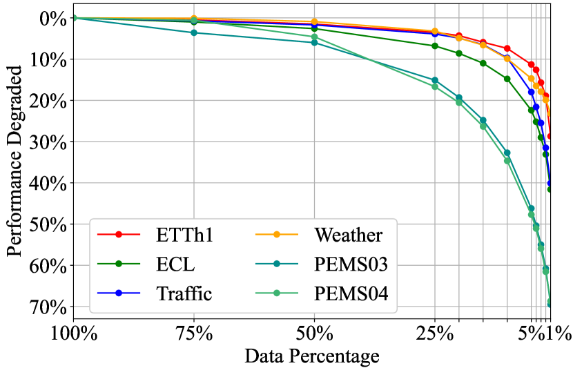
Figure 1: Performance of PatchTST (2022) learned from subset of the training set, evaluated by a decreasing percentage of the subset.

Further, large models evolved by generative pre-training (GPT) have demonstrated several essential abilities that are not present in small models: generalization ability that one model fits all domains, task generality that one model copes with various tasks, and scalability that the performance increases with the scale of parameters and pre-trained data. The endowed capabilities have fostered the advancement of artificial general intelligence (OpenAI, 2023). Time series holds the comparable practical value to natural language. Essentially, they exhibit inherent similarities in generative modeling (Bengio et al., 2000) and autoregression (Box, 2013). Consequently, the unprecedented success of the generative pre-trained large language models (Zhao et al., 2023) serves as a blueprint for the progress of LTSMs.

Although unsupervised pre-training for time series has been widely explored, yielding breakthroughs based on the masked modeling (Zerveas et al., 2021) and contrastive learning (Woo et al., 2022), existing research has not addressed several fundamental issues for developing LTSMs. Firstly, when is the benefit of LTSMs warranted? As is shown in Figure 1, training on $5\%$ samples from ETTh1 only induces a $11\%$ MSE increase. While real-world applications can be data-scarce, the training oversaturation of these benchmarks can underestimate the advantages of LTSMs. Secondly, how to pre-train scalable LTSMs? Though deep learning flourishes the model design for time series, there is no consensus on the LTSMs architecture. And the evidence is still obscure whether existing large-scale pre-trained time series models (Dooley et al., 2023; Woo et al., 2023) with the prevalent encoder-only structure can deliver the expected scalability. Thirdly, the collection and well-established tokenization of heterogeneous time series for pre-training are left behind by other fields. Finally, the unified formulation to tackle various analysis tasks with time series of different lengths by one single pre-trained model remains an underexplored problem for utilizing LTSMs.

In this paper, we propose Timer, together with a thorough suite of pre-training and applicative solutions of large time series models. By aggregating publicly available time series datasets and following curated data processing, we construct Unified Time Series Dataset (UTSD) of hierarchical capacities to facilitate the research on the scalability of LTSMs. To acquire natively pre-trained models on time series, we propose the single-series sequence (S3) format to convert heterogeneous series with reserved patterns into unified token sequences. To realize the few-shot capability and task generality toward LTSMs, we adopt the GPT-style objective that predicts the next token (Bengio et al., 2000). Benefiting from the data, training strategy, and model architecture, we present Timer, a large-scale pre-trained Time Series Transformer. Unlike prevalent encoder-only architecture (Nie et al., 2022; Das et al., 2023a), Timer aligns similar properties as large language models such as the decoder-only structure trained by autoregressive generation. It also presents notable few-shot generalization, scalability, and feasibility for various series lengths and tasks with one model. Overall, our contributions can be summarized as follows:

• Motivated by the emergence of large models in other fields, we advocate the advancement of large time series models for widespread data-scarce scenarios.

• We delve into the LTSM development by curating large-scale datasets comprised of 1B time points, proposing the training strategy with the single-series sequence format, and presenting Timer, a pre-trained decoder-only Transformer for time series analysis at scale.

• We apply Timer on various tasks, which is realized in our unified generative approach. Timer exhibits notable scalability and generalization in each task and achieves state-of-the-art performance with few samples.

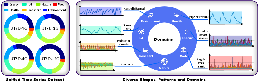
Figure 2: Illustration of Unified Time Series Dataset (UTSD), that is composed of various time series domains with hierarchical capacities.

2 Related Work

2.1 Unsupervised Pre-training on Sequences

Unsupervised pre-training on large-scale data is the essential step for modality understanding for downstream applications, which has achieved substantial success in sequences, covering natural language (Radford et al., 2021), patch-level image (Bao et al., 2021) and video (Yan et al., 2021). Supported by powerful backbones (Vaswani et al., 2017) for sequential modeling, the paradigms of unsupervised pre-training on sequences have been extensively studied in recent years, which can be categorized into the masked modeling (Devlin et al., 2018), contrastive learning (Chen et al., 2020), and generative modeling (Radford et al., 2018).

Inspired by the significant success achieved in other fields, masked modeling and contrastive learning have been well-developed for time series. TST (Zerveas et al., 2021) and PatchTST (Nie et al., 2022) adopt the BERT-style masked pre-training to reconstruct several time points and patches respectively. LaST (Wang et al., 2022b) proposes to learn the representations of decomposed time series based on variational inference. Contrastive learning is also well incorporated in prior works (Woo et al., 2022; Yue et al., 2022). TF-C (Zhang et al., 2022) constrains the time-frequency consistency by temporal variations and frequency spectrums. SimMTM (Dong et al., 2023) combines masked modeling and contrastive approach within the neighbors of time series.

However, the generative pre-training has received relatively less attention in the context of time series despite the prevalence witnessed in developing large language models (Touvron et al., 2023; OpenAI, 2023). Autoregressive generation represents the fundamental commonality between language modeling (Bengio et al., 2000) and time series forecasting, as well as the essential concept of autoregressive forecasters (Box, 2013) that is applicable to arbitrary forecast lengths. Furthermore, prior studies (Wang et al., 2022a; Dai et al., 2022) have demonstrated that model scalability and generalization ability largely stem from the generative pre-training, which necessitates a greater amount of training data. Therefore, our work aims to revitalize generative pre-training at scale towards LTSMs, supported by massive time series and an elaborately designed training strategy.

2.2 Large Time Series Models

Pre-trained models endowed with scalability can evolve to large models (Bommasani et al., 2021), represented as improved model capacity for downstream tasks through scaling the model size or pre-trained data. Large language models even demonstrate advanced capabilities such as in-context learning and emergent abilities (Zhao et al., 2023). Until now, research on large time series models is still in the early stages. Existing works towards LTSMs can be categorized into two groups, with one being large language models for time series. FPT (Zhou et al., 2023) utilizes GPT-2 as a representation extractor of sequences, which is then adapted for general time series analysis. LLMTime (Chang et al., 2023) encodes time series into numerical tokens for LLMs, exhibiting model scalability in the forecasting task. Time-LLM (Jin et al., 2023) investigates prompting techniques to enhance prediction, demonstrating the generalization ability of LLMs. Unlike the above methods, the proposed Timer is pre-trained natively on time series, free from modality alignment, and conducive to downstream tasks of time series.

Another category is large-scale pre-trained models on time series. ForecastFPN (Dooley et al., 2023) proposes to pre-train on synthetic time series data for zero-shot forecasting. CloudOps (Woo et al., 2023) adopts the masked encoder of Transformer towards the domain-specific pre-trained forecaster. Lag-Llama (Rasul et al., 2023) aims to build a scalable univariate forecasting model by pre-training on existing time series benchmarks. PreDcT (Das et al., 2023b) utilizes the decoder-only Transformer pre-trained on diverse time series from Google Trends, exhibiting the zero-shot capability on forecasting benchmarks. Different from the prior works, Timer is pre-trained extensively on 1 billion real-world time points from various domains on the one hand. On the other hand, Timer is applicable to downstream tasks beyond forecasting, capable of tackling variable series lengths, and exhibits scalability towards large models.

3 Approach

Similar to natural language that possesses a sequential structure, we draw upon the technical advancement of large language models as the blueprint. In this paper, we advocate the development for large time series models (LTSM): (1) the utilization of extensive time series corpora, (2) the adoption of a standardized format for diverse time series data, and (3) the pre-training objective on the decoder-only Transformer that autoregressively predict the next time series token.

3.1 Data

Large-scale datasets are of paramount importance for pre-training large models. However, the collection of time series datasets can be prohibitively challenging. Despite the ubiquity of time series in real-world applications, there are numerous data of low quality, including missing values, unpredictability, variance in shape, and irregular sampling intervals, which can significantly impact the efficacy of pre-training. Therefore, we establish the acceptance criteria for filtering high-quality time series data based on extensively collected publicly available datasets. Concretely, we record the statistics of each dataset, including (1) basic properties, such as the number of time steps, variates, file size, interval granularity, etc; and (2) time series characteristics: periodicity, stationarity, and predictability. This also allows us to assess the complexity of different datasets and progressively conduct scalable pre-training. Furthermore, to facilitate the research on domain-specific pre-trained time series models, we differentiate the datasets into typical domains.

We curate Unified Time Series Dataset (UTSD) as shown in Figure 2. UTSD is constructed with hierarchical capacities to facilitate scalability research on the pre-training data size. Currently, UTSD encompasses 7 domains with up to 1 billion time points (UTSD-12G), covering typical scenarios of time series analysis. Following the principle of keeping pattern diversity, we include as assorted datasets as possible in each hierarchy, ensure the data size of each domain is nearly balanced when scaling up, and the complexity gradually increases in accordance with the calculated statistics. Detailed construction and statistics are provided in Appendix A.

3.2 Training Strategy

Different from natural language, which has been facilitated by the well-established discrete tokenization and sequential structure with the regular shape, constructing unified time series sequences is not straightforward due to the heterogeneity of series such as amplitude, frequency, stationarity, and disparities of the datasets in the variate number, series length and purpose. To facilitate pre-training on extensive time series, we propose to convert heterogeneous time series into single-series sequence (S3), which reserves the patterns of series variations with the unified context length.

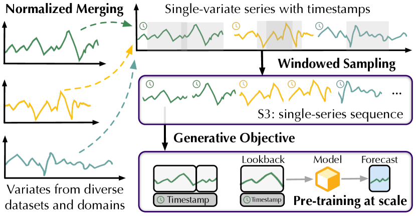
Figure 3: Pre-training strategy for heterogeneous time series.

As depicted in Figure 3, our initial step involves normalizing and merging at the level of variates. Each series representing a variate will be divided into training and validation splits at a ratio of 9:1 for pre-training. We apply the statistics of the training split to normalize the entire series. The normalized time series, along with corresponding timestamps, are then merged into a pool of single-variate series. The time points of single-variate series for training follow the normal distribution, which mainly mitigates the discrepancies in the amplitude and variate numbers across multiple datasets.

We uniformly sample sequences from the pool by a window, obtaining single-series sequences with a fixed length, as the format of S3. Our format is essentially the extension of Channel Independence CI (Nie et al., 2022). However, CI necessitates time-aligned multivariate series and flattens the variate dimension to the same batch, thereby requiring the batch of series to originate from the same dataset. Based on our format, the model observes sequences from different periods and different datasets, thus increasing the pre-training difficulty and directing more attention to temporal variations. The S3 format does not require time-aligned series, making it applicable to widespread univariate and irregular series. It also encourages the large model to capture multivariate correlations from the pool of single-variate series.

We leverage the expertise of developing large language models and employ generative modeling as the pre-training objective, manifested as the forecasting task. This approach differs from contrastive learning and masked modeling widely used in previous unsupervised time series methods.

3.3 Model Design

As language models autoregressively predict the next token:

$$P(\mathcal{U})=\prod_{i=1}^{N}p(u_{i}|u_{<i})$$ (1)

on the token sequence $\mathcal{U}=\{u_{1},\dots,u_{N}\}$, we first establish the tokenization of the given single-series sequence (S3) $\mathbf{X}=\{x_{1},\dots,x_{NS}\}$ with the unified context length $NS$. We define the time series token as consecutive time points (segment) of length $S$ that encompass the series variations:

$$\mathbf{s}_{i}=\{x_{(i-1)S+1},\dots,x_{iS}\}\in\mathbb{R}^{S}.$$ (2)

We adopt the decoder-only Transformer with dimension $D$ and $L$ layers for generative pre-training (GPT) on the $N$ tokens from a single-series sequence:

$$\mathbf{h}_{i}^{0} =\mathbf{W}_{e}\mathbf{s}_{i}+\mathbf{TE}_{i},\ i=1,\dots,N,$$ (3)

$$\mathbf{H}^{l} =\operatorname{TrmBlock}(\mathbf{H}^{l-1}),\ l=1,\dots,L,$$

$$\{\hat{\mathbf{s}}_{i+1}\} =\mathbf{H}^{L}\mathbf{W}_{d},\ i=1,\dots,N,$$

where $\mathbf{W}_{e},\mathbf{W}_{d}\in\mathbb{R}^{D\times S}$ encode and decode token embeddings $\mathbf{H}=\{\mathbf{h}_{i}\}\in\mathbb{R}^{N\times D}$, and $\mathbf{TE}_{i}$ denotes the corresponding (optional) timestamp embedding. Via the causal attention of the decoder-only Transformer, the autoregressively generated $\hat{\mathbf{s}}_{i+1}$ is obtained as the next token of $\mathbf{s}_{i}$. Thus, we formulate the pre-training objective as follows:

$$\mathcal{L}_{\text{MSE}}=\frac{1}{NS}\sum||\mathbf{s}_{i}-\hat{\mathbf{s}}_{i}||_{2}^{2},\ i=2,...,N+1.$$ (4)

We opt for Transformer as the backbone of Timer since it has solidified itself as the predominant scalable choice in other fields. We also evaluate backbone alternatives on time series in Section 4.5. Furthermore, we review Transformer-based models in time series forecasting, which have undergone significant development in recent years. Existing approaches are categorized into encoder-only and decoder-only architectures following the same pipeline. As depicted in Figure 4, prevalent deep forecasters with the encoder-only structure obtain the predicted tokens through flattening and projection. While direct projection may benefit from end-to-end supervision, flattening can also wipe out token dependencies modeled by attention, thereby weakening Transformer layers to reveal the patterns of temporal variations.

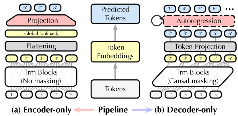
Figure 4: Architectures of typical Transformer-based forecasters.

Therefore, we refer to the substantial progress of large language models integrated with the decode-only architecture. Objective as Equation 4 yields token-wise supervising signals, including additional utilization of the lookback series. Autoregression also provides the flexibility to address variable context length by simply sliding the series at inference. More importantly, the generalization ability is guaranteed by the decoder-only structure in LLMs (Wang et al., 2022a). In a nutshell, we establish LLM-style decoder-only Timer with autoregressive generation pre-training towards LTSMs.

4 Experiments

We demonstrate Timer as a large time series model in time series forecasting, imputation, and anomaly detection by tackling them in a unified generative scheme, which is detailed in the following sections. We also compare Timer with state-of-the-art approaches and present pre-training benefits on data-scarce scenarios, known as the few-shot ability of large models. Furthermore, we delve into the scalability, including the model size and data size. We also explore candidate backbones and architectures towards LTSMs, exhibiting the effectiveness of our architectural option. All downstream datasets evaluated in the experiment are not included in UTSD to prevent data leakage. We provide the detailed implementation and model configurations of pre-training and fine-tuning in Appendix B.1 and Appendix B.2.

4.1 Time Series Forecasting

Setups

Time series forecasting is essential and presents challenges in real-world applications. To thoroughly evaluate the performance, we elaborately establish the benchmark, including ETT, ECL, Traffic, Weather, and PEMS adopted in Liu et al. (2023). We adopt the unified lookback length as $672$ and the forecast length as $96$. We pre-training Timer on UTSD-12G with the segment length $S=96$ and the number of tokens $N=15$, such that Timer can deal with time series with the context length up to $1440$. And the downstream forecasting task is naturally converted into the next token prediction as detailed in Appendix B.2.

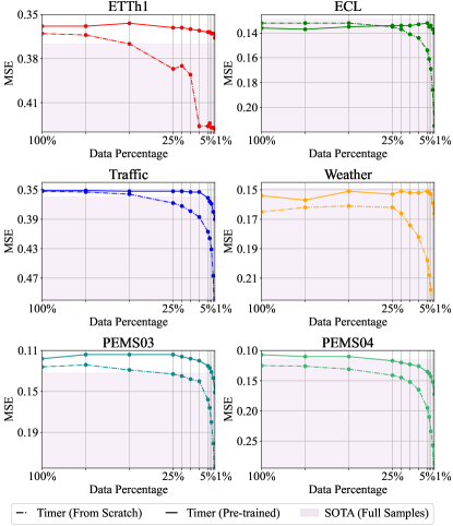
Figure 5: Downstream forecasting results of Timer obtained by training from scratch and fine-tuning from the pre-trained model. The detailed results are provided in Table 7.

Results

As depicted in Figure 5, we present the results of the pre-trained Timer (solid line) and Timer trained from scratch (dashed line) under different data scarcities. Additionally, we also present previous state-of-the-art forecasters trained on full samples, that is, PatchTST (Nie et al., 2022) on ETTh1 and Weather; and iTransformer (Liu et al., 2023) on other datasets, as a competitive baseline. It is notable that the pre-trained Timer demonstrates superior performance to the baseline in four datasets with limited samples, specifically achieving better results with only $1\%$ available samples from ETTh1, $5\%$ from Traffic, $3\%$ from PEMS03, and $25\%$ from PEMS04 with remarkable few-shot ability.

Moreover, the pre-trained Timer exhibits impressive generalization capability through large-scale pre-training, which significantly outperforms the model trained from scratch. Concretely, the performance of training on the entire downstream dataset can be achieved by leveraging only $2\%$ of the training samples in ETTh1, $5\%$ in ECL, $1\%$ in Weather, and $4\%$ in PEMS03, which exemplifies the transferable knowledge acquired during pre-training on UTSD. Further promotions are achieved by training on all available samples in several undersaturated datasets: the forecasting error is reduced as $0.165\to 0.154$ on Weather, $0.126\to 0.118$ on PEMS03, and $0.125\to 0.107$ on PEMS04. Overall, the performance decline of pre-trained Timer is notably less pronounced with increased data scarcity, thereby alleviating the demand for downstream training samples.

4.2 Imputation

Setups

Imputation is widely required in real-world applications, aiming to fill the corrupted time series based on the observed data. However, while various machine learning algorithms and simple linear interpolation can effectively cope with the corruptions randomly happening at the point level, real-world corruptions typically result from prolonged monitor shutdowns and require a continuous period of recovery. Consequently, imputation can be ever challenging when attempting to recover a span of time points encompassing intricate series variations. In this task, we conduct the segment-level imputation. Each time series is divided into $8$ segments and each segment has the length of $24$ and the possibility of being completely masked. We obtain Timer on UTSD-4G by generative pre-training with the segment length $S=24$ and the token number $N=15$. For downstream adaptation, we conduct the denoising autoencoding in T5 (Raffel et al., 2020) as detailed in Appendix B.2 to recover the masked spans in an autoregressive way.

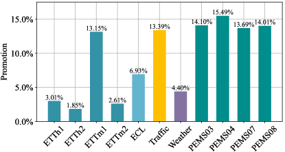
Figure 6: Pre-training benefit of Timer on $5\%$ available samples. We adopt mask ratios in $\{12.5\%,25\%,37.5\%,50\%\}$ and report the average results. Additional results are provided in Figure 14.

Results

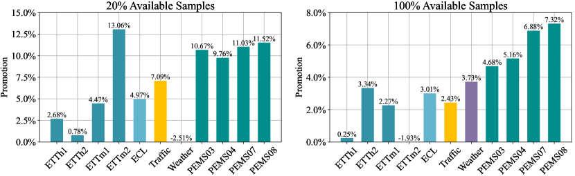
Figure 14: Pre-training benefit of Timer on downstream imputation task with $20\%$ and $100\%$ available samples.The complete data details used to calculate the pre-training benefits relative to training from scratch in this figure are listed in Table 9 and 10.

We conduct experiments on the same datasets of forecasting. As pre-training consistently yields positive effects on all datasets, we show the promotion as the reduction ratio of the imputation error in Figure 6. Additional results in Figure 14 also demonstrate remarkable error reduction with $20\%$ and $100\%$ available samples. We also evaluate previous state-of-the-art TimesNet (Wu et al., 2022) in Table 11 on the segment-wise imputation, where Timer outperforms TimesNet in respectively $100.0\%$, $86.4\%$, and $56.8\%$ of $44$ imputation settings under the same data-scarcities of $\{5\%,20\%,100\%\}$, validating the effectiveness of Timer for the challenging segment-level imputation.

4.3 Anomaly Detection

Setups

Anomaly detection is vital in industry and operations. Previous methods (Xu et al., 2021; Wu et al., 2022) generally adopt the reconstructive approach to tackle the unsupervised scenario, where a feature extractor is trained to reconstruct input series and the output is regarded as standard values. Based on our generative model, we cope with anomaly detection in a predictive approach. The core is to use the observed segments to predict the future segment, and the predicted segment will be established as the standard to be compared with the actual value received. Unlike previous methods requiring to collect time series of a period for reconstruction, our predictive approach allows for segment-level anomaly detection on the fly. Consequently, the task is converted into a forecasting task as detailed in Appendix B.2. The performance is evaluated on UCR Anomaly Archive (Wu & Keogh, 2021), where the task is to find the position of an anomaly in the test series based on a single normal series for training. We use the MSE between the predicted segment and ground truth as the confidence level.

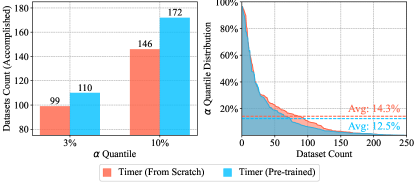
Figure 7: Downstream anomaly detection results of Timer obtained by training from scratch and adapting with the pre-trained model.

Results

We calculate the confidence of all segments on the test set and sort them. If the segment with the $\alpha$ quantile hits the anomaly position labeled in the dataset, it accomplishes the detection of the anomaly. Figure 7 compares the detection performance of pre-trained models and from scratch using two indicators. The left figure shows the number of datasets that the model has completed detection within the quantile of $3\%$ and $10\%$, while the right figure shows the quantile distribution and averaged quantile of all UCR datasets, where the pre-trained Timer with the smaller averaged quantile works as a more accurate detector.

4.4 Scalability

Scalability is the essential property that emerges from pre-trained models to large models. To investigate the scaling behavior of Timer, we conduct extensive pre-training with increased model size and data size as detailed in Table 4 and adapt for downstream forecasting on all subsets of PEMS.

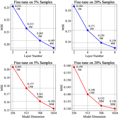
Figure 8: Larger Timer demonstrates better performance on downstream forecasting. Models are all pre-trained on UTSD-4G. Detailed results of all PEMS subsets are provided in Table 13.

Model size

We keep UTSD-4G as the pre-training corpus. The results are depicted in the Figure 8. While maintaining a unified model dimension $D=256$, we increase the number of layers, yielding pre-trained models with parameters ranging from 1M to 4M. It leads to the reduction in forecasting errors of the two few-shot scenarios by an average of $14.7\%$ and $20.6\%$ respectively. Again, we continue to increase the model dimension under the layer number $L=6$ and enlarge the parameters from 3M to 50M, leading to further improved performance by $25.1\%$ and $18.2\%$, validating the effect of scaling up the model size.

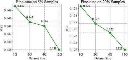
Figure 9: Timer trained on larger dataset demonstrates better performance on downstream forecasting. Models are configured with $L=8$ and $D=1024$. Detailed results are provided in Table 13.

Data size

We pre-train Timer under the unified model size with different UTSD sizes, which exhibits steady improvement with the enlarged pre-training scale in Figure 9. The benefit is relatively small compared to expanding the model size from the beginning, which could be attributed to the performance saturation on this benchmark. Compared with large language models, the parameters of Timer can be still small, indicating the higher parameter efficiency in the time series modality, which is also supported by prior works (Das et al., 2023b). As the scaling law (Kaplan et al., 2020) of large models highlights the significance of synchronized scaling of data with the model parameters, there is still an urgent need to accelerate the data infrastructure in the time series field to promote the development of LTSMs.

Overall, by increasing the parameters and pre-training scale, Timer achieves $0.231\to 0.138\ (-40.3\%)$ and $0.194\to 0.123\ (-36.6\%)$ under few-shot scenarios, even surpassing the performance of the previous state-of-the-art (Liu et al., 2023) training on full samples of PEMS datasets $(0.139)$.

4.5 Analysis

Backbone for LTSM

Deep learning approaches have brought the boom of time series analysis, with various backbones for modeling the sequential time series modality being proposed. To validate the appropriate option for large time series models, we compare Timer with four candidates: MLP-based TiDE (Das et al., 2023a), CNN-based TCN (Bai et al., 2018), RNN-based LSTM (Hochreiter & Schmidhuber, 1997) and encoder-only PatchTST (Nie et al., 2022).

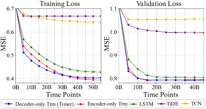
Figure 10: Training loss of candidate backbones. Model dimension and layer number are consistently chosen for a fair comparison.

We apply the unified model configuration and training strategy to pre-train the candidates on UTSD-4G. The loss curves of training and validation are provided in Figure 10, which confirms that Transformer exhibits excellent scalable ability as the backbone for large time series models, whereas MLP-based and CNN-based architectures may encounter the bottleneck in accommodating diverse time series data.

Decoder-only v.s. Encoder-only

While a smaller training loss is achieved by the encoder-only Transformer in Figure 10, the progress of large language models indicates that decoder-only models may possess stronger generalization capabilities in downstream adaptation (Wang et al., 2022a; Dai et al., 2022), which is the essential purpose of LTSMs. Therefore, we further compare the forecasting performance when adapted to different levels of data scarcity.

We elaborately evaluate the performance on six benchmarks in Table 1. By training from scratch, the encoder-only Transformer achieves better end-to-end performance in undersaturated scenarios (1% Target - None), while the decoder-only architecture requires more samples by training from scratch. However, after pre-training, Timer as the decoder-only Transformer exhibits significantly better generalization than the encoder-only pre-trained model, thereby enhancing the performance on most downstream scenarios. The observation partially elucidates why the encoder-only structure has become prevalent in the mainstream time series forecasting field; namely, the encoder-only model is more suitable for small benchmarks, while the decoder-only architecture, which is endowed notable generalization ability and model capacity, is a more suitable choice for developing LTSMs.

Table 1: Downstream forecasting results under different data scarcity of the encoder-only and decoder-only Transformer respectively pre-trained on UTST-12G. Datasets are ordered by the oversaturation in Figure 1. Full results of PEMS and ETT can be found in Table 14.

Scenario	1% Target				5% Target				20% Target
Architecture	Encoder		Decoder		Encoder		Decoder		Encoder		Decoder
Pre-trained	None	12G	None	12G	None	12G	None	12G	None	12G	None	12G
PEMS (Avg)	0.286	0.246	0.328	0.180	0.220	0.197	0.215	0.138	0.173	0.164	0.153	0.126
ECL	0.183	0.168	0.215	0.140	0.150	0.147	0.154	0.132	0.140	0.138	0.137	0.134
Traffic	0.442	0.434	0.545	0.390	0.392	0.384	0.407	0.361	0.367	0.363	0.372	0.352
ETT (Avg)	0.367	0.317	0.340	0.295	0.339	0.303	0.321	0.285	0.309	0.301	0.297	0.288
Weather	0.224	0.165	0.246	0.166	0.182	0.154	0.198	0.151	0.153	0.149	0.166	0.151

Table 2: In-domain and out-of-domain forecasting results by pre-training on the source domain and fine-tuning on the target dataset under different data scarcity. ECL and Weather belong to the Energy and Nature domains respectively.

Target Dataset	Weather						ECL
Source Domain	From Scratch		Energy		Nature		From Scratch		Nature		Energy
Metric	MSE	MAE	MSE	MAE	MSE	MAE	MSE	MAE	MSE	MAE	MSE	MAE
5% Target	0.229	0.279	0.171	0.220	0.162	0.212	0.179	0.277	0.165	0.269	0.141	0.238
20% Target	0.185	0.238	0.160	0.212	0.153	0.202	0.145	0.243	0.140	0.238	0.133	0.228
100% Target	0.158	0.209	0.152	0.199	0.151	0.198	0.130	0.224	0.132	0.224	0.131	0.223

Flexible sequence length

The decoder-only architecture provides additional flexibility to accommodate series of different lengths. For example, Timer can handle variable lookback lengths less than the context length, since it has been supervisedly trained on each context length during pre-training as Equation 4, thereby achieving enhanced performance by the increasing lookback length in Figure 11. It can also generate arbitrary tokens as the prediction by autoregressively sliding. By contrast, realizing this by encoder-only models with the rigid context length would necessitate rolling forecasting, leading to significant error accumulation, which is illustrated at the bottom of Figure 11.

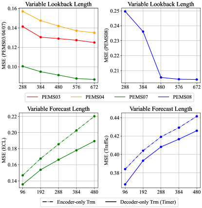
Figure 11: Performance of Timer on variable context length.

Domain transfer

To investigate the effectiveness of domain partitioning of UTSD, we examined the results of adopting different domains of UTSD as the source and adapting to different target datasets to establish in-domain and out-of-domain transfer. The results in Table 2 indicate that in-domain transfer can further enhance the downstream performance. Additionally, as the number of downstream data samples increases, the relative improvement of pre-training will gradually diminish, and even lead to negative transfer in some out-of-domain scenarios. It provides a promising direction to develop domain-specific pre-trained models.

5 Conclusion

Time series analysis scenarios increasingly underscore the demand for large time series models. In this paper, we construct time series corpora from diverse domains, standardize them into a unified sequence format, and utilize a generative objective to pre-train a decoder-only Transformer, presenting a scalable, task-agnostic Timer for time series analysis. Experimentally, we evaluate the generality of Timer in forecasting, imputation, and anomaly detection, yielding remarkable downstream results and notable pre-training benefits in data-scarce scenarios. Further analysis validates the model scalability and effectiveness of architecture, and flexibility to tackle variable series lengths. In the future, we will continue to scale up the datasets and Timer, as well as explore advanced capabilities of LTSMs, such as the zero-shot generalization and in-context learning ability, to address a wider range of time series analysis tasks.

Appendix A Unified Time Series Dataset

A.1 Datasets Details

Unified Time Series Dataset (UTSD) is meticulously assembled from a blend of publicly accessible online data repositories and empirical data derived from real-world machine operations. To enhance data integrity, missing values are systematically addressed using linear interpolation techniques. We follow the unified data storage format used in Autoformer (Wu et al., 2021). For each univariate, multivariate and irregular-sampled time series, we align the time series with timestamps and store them in one single CSV file. One dataset may composed of multiple related time series. UTSD encompasses a collection of 29 individual datasets as listed in Table 3, intricately representative of a wide range of domains.

All datasets are classified into seven distinct domains by their source: Energy, Environment, Health, Internet of Things (IoT), Nature, Transportation, and Web. Datasets of UTSD exhibit diverse sampling frequencies, ranging from macro intervals such as yearly and quarterly to more fine-grained intervals like hourly and minutely. Notably, several datasets can demonstrate exceptionally high-frequency sampling rates, such as the MotorImagery dataset, which operates at a millisecond frequency.

In the pursuit of advanced data analysis, we have also analyzed the stationarity manifested as ADF test statistics (Elliott et al., 1996) and forecastability (Goerg, 2013). The rigorous methodologies and intricate details are elaborated in Section A.2.

Table 3: Dataset detailed descriptions. Time Point denotes the total number of time points aggregating from all variates if multivariate. File Size denotes the storage that the CSV file of the dataset occupies. Freq. denotes the sampling interval of time points, where “-” indicates no timestamp or irregular interval. ADF. denotes the Augmented Dickey-Fuller test statistics of the dataset. Forecast. denotes the forecastability of the dataset. Source denotes the original paper or resource of the dataset.

Domain	Dataset	Time Points	File Size	Freq.	ADF.	Forecast.	Source
Energy	London Smart Meters	166.50M	4120M	Hourly	-13.158	0.173	Godahewa et al. (2021)
	Wind Farms	7.40M	179M	4 sec	-29.174	0.811	Godahewa et al. (2021)
	Aus. Electricity Demand	1.16M	35M	30 min	-27.554	0.730	Godahewa et al. (2021)
Environment	AustraliaRainfall	11.54M	54M	Hourly	-150.10	0.458	Tan et al. (2021)
	BeijingPM25Quality	3.66M	26M	Hourly	-31.415	0.404	Tan et al. (2021)
	BenzeneConcentration	16.34M	206M	Hourly	-65.187	0.526	Tan et al. (2021)
Health	MotorImagery	72.58M	514M	0.001 sec	-3.132	0.449	Dau et al. (2019)
	SelfRegulationSCP1	3.02M	18M	0.004 sec	-3.191	0.504	Dau et al. (2019)
	SelfRegulationSCP2	3.06M	18M	0.004 sec	-2.715	0.481	Dau et al. (2019)
	AtrialFibrillation	0.04M	1M	0.008 sec	-7.061	0.167	Dau et al. (2019)
	PigArtPressure	0.62M	7M	-	-7.649	0.739	Dau et al. (2019)
	PigCVP	0.62M	7M	-	-4.855	0.577	Dau et al. (2019)
	IEEEPPG	15.48M	136M	0.008 sec	-7.725	0.380	Tan et al. (2021)
	BIDMC32HR	63.59M	651M	-	-14.135	0.523	Tan et al. (2021)
	TDBrain	72.30M	1333M	0.002 sec	-3.167	0.967	Wang et al. (2023)
IoT	SensorData	165.4M	2067M	0.02 sec	-15.892	0.917	Real-world machine logs
Nature	Phoneme	2.16M	25M	-	-8.506	0.243	Dau et al. (2019)
	EigenWorms	27.95M	252M	-	-12.201	0.393	Dau et al. (2019)
	ERA5 Surface	58.44M	574M	3 h	-28.263	0.493	Muñoz-Sabater et al. (2021)
	ERA5 Pressure	116.88M	1083M	3h	-22.001	0.853	Muñoz-Sabater et al. (2021)
	Temperature Rain	23.25M	109M	Daily	-10.952	0.133	Godahewa et al. (2021)
	StarLightCurves	9.46M	109M	-	-1.891	0.555	Dau et al. (2019)
	Saugeen River Flow	0.02M	1M	Daily	-19.305	0.300	Godahewa et al. (2021)
	KDD Cup 2018	2.94M	67M	Hourly	-10.107	0.362	Godahewa et al. (2021)
	US Births	0.00M	1M	Daily	-3.352	0.675	Godahewa et al. (2021)
	Sunspot	0.07M	2M	Daily	-7.866	0.287	Godahewa et al. (2021)
	Worms	0.23M	4M	0.033 sec	-3.851	0.395	Dau et al. (2019)
Transport	Pedestrian Counts	3.13M	72M	Hourly	-23.462	0.297	Godahewa et al. (2021)
Web	Web Traffic	116.49M	388M	Daily	-8.272	0.299	Godahewa et al. (2021)

A.2 Statistics

We analyze each dataset within our collection, examining the time series through the lenses of stationarity and forecastability. This approach allows us to characterize the level of complexity inherent to each dataset.

Stationarity

The stationarity of time series is a fundamental property that can be rigorously quantified using the Augmented Dickey-Fuller (ADF) test. Notably, a larger ADF test statistic typically signifies a higher degree of non-stationarity within the time series (Elliott et al., 1996). In the context of datasets comprising multiple time series, the challenge of aligning these series arises, particularly when they vary in length. To address this, we implement a length-weighted ADF method that evaluates the stationarity of the entire dataset, taking into consideration the varying lengths of individual series. This approach ensures that the contribution of each series to the overall stationarity metric is proportional to its length, thus reflecting its relative significance within the dataset. By doing so, the length-weighted ADF provides a more granular and accurate depiction of the stationarity of the dataset, highlighting the impact of longer series on the overall stability and ensuring that shorter series do not disproportionately affect the assessment. The weighted statistic is formulated as follows:

$$T=\sum_{i=1}^{C}T_{i},\ \operatorname{ADF-Statistic}(\mathcal{D})=\sum_{i=1}^{C}\frac{T_{i}}{T}\operatorname{ADF-Statistic}(\mathbf{S}^{(i)}),$$ (5)

where $\mathbf{S}_{i}\in\mathbb{R}^{T_{i}}$ denotes the $i$-th series in dataset $\mathcal{D}$, $T_{i}$ is the length of $\mathbf{S}_{i}$ and $C$ is the number of time series of dataset $\mathcal{D}$.

Forecastability

Forecastability is calculated by subtracting the entropy of the series Fourier decomposition adopted from Goerg (2013), where a higher forecastability value indicates superior predictability. Just as with the assessment of stationarity, when considering a dataset composed of multiple time series of varying lengths, it is essential to adjust the measure of forecastability to account for these differences. Therefore, we extend the concept of forecastability to a weighted version, analogous to the length-weighted ADF method, to finely tune the predictability assessment to the individual characteristics of each series. The weighted forecastability for a dataset can be formulated as follows:

$$T=\sum_{i=1}^{C}T_{i},\ \operatorname{Forecastability}(\mathcal{D})=\sum_{i=1}^{C}\frac{T_{i}}{T}(1-\operatorname{Entropy}(\mathcal{F}(\mathbf{S}^{(i)}))),$$ (6)

where $\mathbf{S}_{i}\in\mathbb{R}^{T_{i}}$ denotes the $i$-th time series in dataset $\mathcal{D}$, $T_{i}$ is the length of $\mathbf{S}_{i}$ and $C$ is the number of time series in dataset $\mathcal{D}$. $\mathcal{F}(\mathbf{S}^{(i)})$ denotes the Fourier decomposition of series $\mathbf{S}^{(i)}$.

A.3 UTSD Composition Analysis

UTSD is constructed with hierarchical capacities, namely UTSD-1G, UTSD-2G, UTSD-4G, and UTSD-12G, where each smaller dataset is a subset of the larger ones. We adhere to the principle of progressively increasing the complexity and pattern diversity. Hierarchical structuring allows for a nuanced analysis that accounts for different levels of data granularity and complexity, ensuring that the pattern diversity is maintained across each hierarchy of the dataset. This approach not only facilitates a comprehensive evaluation across different scales but also ensures that each subset within the larger dataset offers a unique and incrementally challenging perspective, thus contributing to a more scalable pre-training.

Dataset Complexity

We conduct a comprehensive analysis of individual datasets to obtain the stationarity and forecastability measures and construct the UTSD hierarchically regarding these indicators. Concretely, based on the ${\operatorname{ADF-Statistic}}$ of each dataset, we categorized the predictive difficulty of the datasets into three distinct levels: Easy, Medium, and Hard. The classification criteria are as follows:

• Easy: ${\operatorname{ADF-Statistic}}<-15.00;$

• Medium: $-15.00\leq{\operatorname{ADF-Statistic}}<-5.00;$

• Hard: $-5.00\leq{\operatorname{ADF-Statistic}}.$

For excessively long datasets in the temporal dimension, we additionally adopt the forecastability to assess the complexity of time series across different periods. As the capacity of UTSD increases, the periods with low forecastability will be further incorporated correspondingly. In a nutshell, larger datasets contain a greater proportion of challenging tasks as shown in Figure 12, thereby escalating the complexity of the pre-training process. The hierarchy reflects an increase in the difficulty of patterns as the dataset size grows. This approach enables a structured examination of the learning challenges presented by different dataset sizes, underlining the intricate balance between data volume and pre-training difficulty.

Figure 12: Dataset complexity in each hierarchy of UTSD.

Pattern Diversity

Each individual dataset within the UTSD collection demonstrates unique patterns, highlighting the importance of maintaining pattern diversity. We build the UTSD dataset in a top-down order, ensuring that each hierarchy within UTSD comprehensively represents all individual datasets and contains as many patterns as possible. As shown in Figure 13, we select several representative datasets for visualization analysis:

• AtrialFibrillation: this dataset showcases a fluctuating trend with minimal seasonality. This pattern is indicative of irregular heart rhythm characteristics, typical in medical recordings related to cardiac health. Such fluctuations, lacking a clear seasonal pattern, are crucial for understanding the unpredictable nature of atrial fibrillation.

• PigArtPressure: this dataset reveals a fluctuating trend interspersed with notable seasonality. This pattern is representative of the physiological variations in blood pressure that can occur due to environmental or internal factors. The presence of both fluctuating trends and seasonality in this dataset underscores the complex nature of biological data.

• US Births: this dataset distinctly exhibits a clear trend alongside pronounced seasonality. This pattern is characteristic of demographic data, where trends and seasonal variations can reflect socio-cultural factors and environmental influences. The consistent trend and seasonality in birth rates provide insights into population dynamics and reproductive behaviors.

Figure 13: Visualization of representative patterns in UTSD. Each time series is decomposed into trend, seasonal, and residual components.

To avoid selecting trivial temporal variations and provide a comprehensive representation of the varied patterns inherent in the individual datasets, we employ a downsampling technique for individual datasets. For those with a larger number of variates, we selectively choose representative variates that best encapsulate the distinct patterns of the respective individual datasets. Similarly, for individual datasets with considerable temporal length, we extract the representative period. This methodical selection process ensures that the integrity and distinctive characteristics of each individual dataset are preserved, thereby maintaining the diversity of patterns across the hierarchical structure of the UTSD dataset.

Appendix B Implementation Details

B.1 Pre-training

Based on the constructed UTSD datasets of different sizes and difficulties in the unified single series sequence (S3) format, Timer is pre-trained with increasing data sizes and model parameters to validate the scalability. The detailed model configurations and parameter count of the pre-trained models involved in this paper are shown in Table 4.

Table 4: Detailed model configurations of Timer and corresponding parameter counts. The number of heads for models of all is fixed as $8$.

Scenario	Model Dim. Scale-up				Layer Number. Scale-up				Others
Scale	3M	13M	29M	51M	1M	2M	3M	4M	38M	67M
Layers	6	6	6	6	2	4	6	8	8	8
Model Dim.	256	512	768	1024	256	256	256	256	768	1024
FFN Dim.	512	1024	1536	2048	512	512	512	512	1536	2048
Parameters	3.21M	12.72M	28.51M	50.59M	1.10M	2.16M	3.21M	4.27M	37.97M	67.40M

All experiments were implemented in PyTorch (Paszke et al., 2019) and trained using NVIDIA A100 Tensor Core GPU. We use AdamW (Kingma & Ba, 2015) as the optimizer and cosine annealing algorithm for learning rate decay. The base learning rate is $5\times 10^{-5}$, and the final learning rate is $2\times 10^{-6}$ . The decay steps are proportional to the number of training steps of 10 epochs. During pre-training, we use $N=15$ as the number of tokens, and the batch size is set to 8192.

During the pre-training on the UTSD-1G to UTSD-4G, we adopt a global shuffle strategy by loading the whole time series into the memory. Due to the much greater data scale of UTSD-12G compared to any commonly used time series dataset in the past, it is difficult to load all 12GB of the pre-training dataset into memory for global shuffling. Therefore, we use a local shuffle strategy, which randomly selects and divides the 12GB pre-training dataset into three 4G subsets in the storage space through file selection and segmentation, and then takes turns loading them into memory for pre-training with global steps. In this strategy, we also ensure the continuity of learning rate decay.

B.2 Downstream Tasks

We introduce the details of downstream experiments and present the generative scheme for each task, including time series forecast, imputation, and anomaly detection. Configurations for downstream adaptation are listed in Table 6. Corresponding detailed results are provided in Section C. And showcases of downstream tasks are shown in Figure 15, 16, and 17.

Forecasting

The downstream forecasting task is tested on five real-world datasets, including (1) ETT (Zhou et al., 2021) contains 7 variates of power transformers, with the period from July 2016 to July 2018, including four subsets and sampling intervals of one hour and fifteen minutes. (2) ECL (Wu et al., 2021) mainly consists of hourly electricity consumption data from 321 customers (3) Traffic (Wu et al., 2021) collected hourly road occupancy rates measured by 862 sensors on the San Francisco Bay Area highway from January 2015 to December 2016. (4) Weather (Wu et al., 2021) consists of 21 meteorological variates collected every 10 minutes from the Max Planck Institute of Biogeochemistry meteorological station in 2020. (5) PEMS contains California public transportation network data collected through a 5-minute window with the same four common subsets (PEMS03, PEMS04, PEMS07, PEMS08) used in SCINet (Liu et al., 2022).

Table 5: Downstream forecasting dataset descriptions. Split denotes the number of time points in (train, validation, test) splits. Frequency denotes the sampling interval of time points. Information denotes the domain in which the dataset belongs to.

Dataset	Variate	Split	Frequency	Information
ETTh1, ETTh2	7	(8545, 2881, 2881)	Hourly	Electricity
ETTm1, ETTm2	7	(34465, 11521, 11521)	15min	Electricity
ECL	321	(18317, 2633, 5261)	Hourly	Electricity
Traffic	862	(12185, 1757, 3509)	Hourly	Transportation
Weather	21	(36792, 5271, 10540)	10min	Weather
PEMS03	358	(15617,5135,5135)	5min	Transportation
PEMS04	307	(10172,3375,281)	5min	Transportation
PEMS07	883	(16911,5622,468)	5min	Transportation
PEMS08	170	(10690,3548,265)	5min	Transportation

We adopt the autoregressive generation training objective (Bengio et al., 2000) for downstream forecasting datasets in the fine-tuning stage. Specifically, we divide the lookback length into $N=7$ tokens with the segment length $S=96$. The model naturally outputs $N$ next tokens, which we calculate the mean squared error (MSE) of the $N$ tokens with corresponding ground truth and backpropagate the loss. During inference, we conduct autoregressive generation by concatenating the forecasted result with the lookback series and repeatedly adopting the model to generate the next token until the total length of predicted tokens reaches the forecasted length (if exceeding the predicted length, we crop the result).

For constructing data-scarce scenarios, we perform retrieval with the uniform interval in the training split according to the sampling ratio and conduct random shuffling at the end of each epoch to train the model. The construction pipeline with the fixed random seed ensures the reproducibility of our experimental results. In order to maintain comparability with previous benchmarks, we keep the same validation and testing sets of original downstream datasets and train the baseline model and Timer with the same set of training samples.

Imputation

Considering the real-world scenario that missing values at time points often appear in succession, we adjust the previous point-level imputation proposed by TimesNet (Wu et al., 2022) and increase the difficulty of the task, that is, changing the masked unit from point to time series segment. The protocol poses challenges to recovering successive points, which underscore higher demands for the model capacity to restore a span of series variations. Concretely, for a time series consisting of $N=8$ segments with a length of $24$, we randomly mask several segments as zeros except for the first segment, ensuring that the first segment is observed by the model to learn about initial series variations for imputation. For the training objective of downstream adaption, we adopt the denoising autoencoding (Raffel et al., 2020), which takes the masked parts as special tokens and unmasked segments as tokens as the model input. Due to the generative capability of Timer acquired by pre-training, we regard outputted tokens as the next predicted tokens and backpropagate the reconstruction error between the generated next token of the masked segment with the ground truth. During inference, we take the MSE of the masked segments as the indicator to evaluate the imputation performance. Based on the above protocol, we conduct the imputation task on the same datasets of the forecasting task in Table 5.

Table 6: Detailed explanation of model hyperparameters and corresponding parameter quantities. We adopt the learning rate schedule strategy with exponential decay at a base of $0.5$ under all three downstream tasks.

Tasks	Model Hyper-parameter				Training Process
	$L_{min}$	$L_{max}$	$d_{min}$ †	$d_{max}$ †	LR∗	Loss	Batch Size	Epochs
Forecasting	2	8	256	2048	3e-5	MSE	2048	10
Imputation	4	4	256	256	3e-5	MSE	32	10
Anomaly Detection	4	4	256	256	3e-5	MSE	128	10

• $\ast$ LR means the initial learning rate.

Anomaly detection

For anomaly detection, prevalent protocols represented by Anomaly Transformer (Xu et al., 2021) and TimesNet (Wu et al., 2022) adopt the reconstructive approach that learns a feature extractor to reconstruct raw series, and the output is regarded as standard values. With all the mean squared errors between the standard and input series from the datasets, a specific threshold with the given quantile is determined to label the anomalies.

Considering the prevalent scenarios of anomaly detection by monitoring real-time measurements, the quick judgment of on-the-fly time series anomaly can be more practical in the real world. Therefore, we propose a predictive protocol of anomaly detection based on generative models. Concretely, we use the observed segments to predict the future segment, and the predicted segment will be established as the standard to be compared with the actual value received. We adopt the UCR Anomaly Archive proposed by Wu & Keogh (2021). The task is to find the position of an anomaly in the test series based on a single normal series for training, which is an extremely data-scarce scenario with only one available sample. For downstream adaption, we adopt the same next token prediction as the pre-training, that is, training Timer with the lookback series containing $N=7$ segments of the length $S=96$ to generate the next token with length $96$, which is regarded as the standard value. After training, we record the MSE of all segments in the test set and sort them in descending order. We find the first segment hit the anomaly interval labeled in the dataset within the first $\alpha$ quantile, and we record the quantile. Based on the above protocol, the real-time judgment ability of the model for sudden anomalies can be predictively examined. With more complex time series anomalies introduced by the UCR Anomaly Archive, we hope to establish a more reasonable and challenging benchmark in the field of anomaly detection.

Appendix C Full Results

C.1 Time Series Forecasting

We provide all the results of the forecasting task in Figure 5. As shown in Table 7, we include six representative real-world datasets, demonstrating that Timer achieves state-of-the-art forecasting performance and the large-scale pre-training helps to alleviate performance degradation as the available downstream samples decrease.

Table 7: Full forecasting results of Timer obtained by training from scratch (None) and fine-tuning from UTSD-12G pre-trained model. The bold values we use indicate that the pre-trained model results have positive benefits compared to from scratch. We attach the current state-of-the-art results as SOTA in this table, including PatchTST (Nie et al., 2022) on ETTh1 and Weather, as well as iTransformer (Liu et al., 2023) on ECL, Traffic, PEMS03, and PEMS04. We adopt the unified lookback length as $672$ and the forecast length as $96$.

Dataset	ETTh1		ECL		Traffic		Weather		PEMS03		PEMS04
Pre-trained	None	12G	None	12G	None	12G	None	12G	None	12G	None	12G
100%	0.363	0.358	0.132	0.136	0.352	0.351	0.165	0.154	0.126	0.118	0.125	0.107
75%	0.364	0.358	0.132	0.137	0.353	0.351	0.162	0.157	0.124	0.114	0.126	0.110
50%	0.370	0.356	0.132	0.135	0.356	0.352	0.161	0.151	0.129	0.114	0.131	0.110
25%	0.387	0.359	0.135	0.134	0.368	0.352	0.162	0.153	0.133	0.114	0.141	0.117
20%	0.385	0.359	0.137	0.134	0.372	0.352	0.166	0.151	0.135	0.116	0.145	0.120
15%	0.391	0.360	0.141	0.134	0.379	0.353	0.174	0.152	0.138	0.118	0.152	0.123
10%	0.426	0.361	0.144	0.133	0.387	0.353	0.182	0.152	0.140	0.120	0.165	0.126
5%	0.426	0.362	0.154	0.132	0.407	0.361	0.198	0.151	0.158	0.125	0.195	0.135
4%	0.424	0.362	0.161	0.135	0.416	0.366	0.208	0.152	0.166	0.127	0.210	0.138
3%	0.427	0.363	0.169	0.134	0.431	0.369	0.218	0.153	0.180	0.131	0.234	0.143
2%	0.427	0.363	0.186	0.137	0.467	0.380	0.230	0.159	0.201	0.137	0.257	0.152
1%	0.428	0.366	0.215	0.140	0.545	0.390	0.246	0.166	0.249	0.151	0.320	0.172
SOTA	0.370		0.129		0.360		0.149		0.132		0.115

C.2 Imputation

In this section, we provide the detailed results of the imputation task, including Timer trained from scratch and adapting pre-trained models with $5\%$ available samples in Table 8, $20\%$ samples in Table 9, and full samples in Table 10 on the downstream task. We also report the results of TimesNet at the above three ratios in Table 11. Based on the result, we provided an improvement in imputation performance before and after pre-training with $\{5\%,20\%,100\%\}$ samples in Figure 6 and 14, reflecting the benefits of autoregressive pre-training in segment-wise imputation task.

Table 8: Downstream imputation with $5\%$ samples. Pre-training benefit $\Delta\%$ is calculated as the ratio of decreased imputing error in MSE. In the case of $5\%$ samples, our pre-trained model outperforms TimesNet (Table 11) in all $44$ settings on datasets and masked ratios.

Mask Ratio	12.5%			25.0%			37.5%			50.0%
Pre-trained	None	12G	$\Delta\%$	None	12G	$\Delta$%	None	12G	$\Delta\%$	None	12G	$\Delta\%$
ETTh1	0.301	0.292	+3.08	0.313	0.299	+4.46	0.322	0.307	+4.59	0.325	0.325	0.00
ETTh2	0.172	0.168	+2.64	0.182	0.180	+1.26	0.197	0.190	+3.22	0.216	0.215	+0.47
ETTm1	0.397	0.347	+12.52	0.403	0.332	+17.72	0.428	0.374	+12.77	0.473	0.425	+10.13
ETTm2	0.118	0.116	+1.59	0.127	0.121	+4.69	0.134	0.131	+2.22	0.147	0.144	+1.99
ECL	0.152	0.140	+7.67	0.162	0.150	+7.27	0.172	0.161	+6.76	0.185	0.174	+6.17
Traffic	0.538	0.460	+14.60	0.567	0.487	+14.14	0.598	0.520	+13.16	0.633	0.558	+11.91
Weather	0.113	0.117	-3.18	0.116	0.114	+2.31	0.128	0.124	+3.28	0.155	0.136	+12.42
PEMS03	0.160	0.135	+15.78	0.196	0.168	+14.60	0.257	0.223	+13.51	0.354	0.306	+13.49
PEMS04	0.193	0.161	+16.80	0.238	0.202	+15.30	0.305	0.258	+15.28	0.410	0.348	+15.14
PEMS07	0.166	0.139	+16.19	0.210	0.183	+12.89	0.278	0.243	+12.72	0.378	0.326	+13.76
PEMS08	0.185	0.157	+15.33	0.232	0.195	+15.98	0.303	0.265	+12.75	0.417	0.362	+13.26

Table 9: Downstream imputation with $20\%$ samples. Pre-training benefit $\Delta\%$ is calculated as the ratio of decreased imputing error in MSE. In the case of $20\%$ samples, our pre-trained model outperforms TimesNet in $86.4\%$ of $44$ settings on datasets and masked ratios.

Mask Ratio	12.5%			25.0%			37.5%			50.0%
Pre-trained	None	12G	$\Delta\%$	None	12G	$\Delta$%	None	12G	$\Delta\%$	None	12G	$\Delta\%$
ETTh1	0.289	0.278	3.83	0.293	0.287	1.91	0.305	0.297	2.56	0.322	0.314	2.44
ETTh2	0.168	0.166	1.21	0.180	0.178	1.02	0.192	0.190	0.73	0.208	0.208	0.17
ETTm1	0.349	0.328	5.98	0.335	0.326	2.72	0.378	0.360	4.84	0.426	0.407	4.34
ETTm2	0.139	0.133	4.77	0.158	0.123	22.30	0.176	0.136	22.95	0.146	0.143	2.22
ECL	0.136	0.130	5.01	0.146	0.138	5.30	0.157	0.149	5.04	0.170	0.162	4.54
Traffic	0.451	0.420	6.89	0.481	0.446	7.26	0.513	0.477	7.09	0.550	0.511	7.10
Weather	0.125	0.129	-3.40	0.125	0.147	-17.46	0.154	0.125	18.77	0.141	0.153	-7.93
PEMS03	0.134	0.120	10.41	0.169	0.150	11.35	0.221	0.198	10.61	0.305	0.273	10.32
PEMS04	0.162	0.146	9.93	0.203	0.184	9.61	0.262	0.236	9.86	0.354	0.320	9.65
PEMS07	0.140	0.125	10.96	0.182	0.162	10.85	0.240	0.214	10.77	0.327	0.290	11.57
PEMS08	0.155	0.139	10.39	0.198	0.174	12.11	0.268	0.236	11.94	0.366	0.324	11.63

Table 10: Downstream imputation with $100\%$ samples. Pre-training benefit $\Delta\%$ is calculated as the ratio of decreased imputing error in MSE. In the case of $100\%$ samples, our pre-trained model outperforms TimesNet in $56.8\%$ of $44$ settings on datasets and masked ratios.

Mask Ratio	12.5%			25.0%			37.5%			50.0%
Pre-trained	None	12G	$\Delta\%$	None	12G	$\Delta$%	None	12G	$\Delta\%$	None	12G	$\Delta\%$
ETTh1	0.274	0.273	0.34	0.283	0.283	-0.04	0.295	0.294	0.52	0.313	0.312	0.17
ETTh2	0.207	0.177	14.44	0.186	0.186	-0.49	0.192	0.195	-1.18	0.210	0.209	0.57
ETTm1	0.342	0.352	-3.04	0.359	0.345	3.87	0.400	0.371	7.09	0.418	0.413	1.15
ETTm2	0.149	0.161	-8.01	0.153	0.171	-11.46	0.173	0.176	-1.53	0.183	0.158	13.27
ECL	0.125	0.122	2.98	0.134	0.130	3.06	0.144	0.139	3.12	0.157	0.152	2.87
Traffic	0.402	0.392	2.50	0.424	0.414	2.48	0.454	0.443	2.46	0.488	0.477	2.29
Weather	0.144	0.157	-8.67	0.159	0.146	8.01	0.162	0.147	9.41	0.168	0.158	6.15
PEMS03	0.113	0.108	4.65	0.143	0.135	5.30	0.188	0.179	4.88	0.258	0.248	3.90
PEMS04	0.142	0.134	5.23	0.176	0.166	5.39	0.227	0.216	5.24	0.311	0.296	4.77
PEMS07	0.121	0.114	5.81	0.155	0.144	6.50	0.204	0.189	7.36	0.277	0.256	7.85
PEMS08	0.137	0.129	5.89	0.169	0.157	7.29	0.224	0.206	7.70	0.314	0.288	8.39

Table 11: Full results of downstream imputation of TimesNet under different data scarcities as the baseline.

Sample Ratio	5%				20%				100%
Mask Ratio	12.5%	25.0%	37.5%	50.0%	12.5%	25.0%	37.5%	50.0%	12.5%	25.0%	37.5%	50.0%
ETTh1	0.676	0.671	0.678	0.682	0.684	0.687	0.675	0.679	0.284	0.296	0.269	0.289
ETTh2	0.258	0.249	0.272	0.276	0.252	0.245	0.251	0.268	0.178	0.199	0.219	0.253
ETTm1	0.665	0.734	0.441	0.483	0.254	0.344	0.314	0.444	0.185	0.232	0.273	0.373
ETTm2	0.138	0.135	0.143	0.153	0.104	0.107	0.119	0.148	0.084	0.090	0.096	0.112
ECL	0.226	0.222	0.230	0.230	0.221	0.224	0.226	0.231	0.200	0.207	0.209	0.211
Traffic	0.802	0.794	0.801	0.809	0.801	0.791	0.798	0.805	0.773	0.775	0.624	0.565
Weather	0.155	0.141	0.162	0.168	0.135	0.124	0.132	0.157	0.104	0.114	0.111	0.127
PEMS03	0.173	0.192	0.239	0.321	0.156	0.291	0.254	0.318	0.142	0.148	0.195	0.273
PEMS04	0.215	0.243	0.291	0.379	0.179	0.222	0.266	0.350	0.123	0.167	0.210	0.285
PEMS07	0.166	0.195	0.247	0.335	0.161	0.195	0.253	0.310	0.113	0.142	0.191	0.272
PEMS08	0.293	0.265	0.346	0.404	0.210	0.214	0.309	0.378	0.147	0.185	0.239	0.326

C.3 Anomaly Detection

In this section, we provide detailed results of anomaly detection in Table 12, including the results of Timer from scratch and from pre-trained. We conducted experiments on all 250 datasets of UCR Anomaly Archive and calculated the corresponding $\alpha$ quantiles. The results show that the pre-trained Timer can detect time series anomalies with lower $\alpha$ on most datasets.

Table 12: Full results of anomaly detection on UCR Anomaly Archive, which contains $250$ datasets (arranged in 25 rows for a total of 10 rows). We provide the quantile ($\%$) of each dataset, where the bold parts represent the better results that benefited from pre-training.

Index		1	2	3	4	5	6	7	8	9	10	11	12	13	14	15	16	17	18	19	20	21	22	23	24	25
Timer (From Scratch)	1	1.1	16.2	6.7	1.2	19.0	23.8	16.7	19.0	14.3	2.4	0.5	13.3	2.0	1.8	0.0	0.4	0.4	30.7	3.0	3.0	7.6	1.3	3.0	47.6	14.3
	2	1.7	81.7	28.3	25.0	2.4	2.1	1.7	3.3	1.7	4.2	13.3	0.4	8.1	8.9	28.5	7.7	89.7	0.7	0.9	22.8	15.3	4.2	2.6	2.6	9.0
	3	5.1	1.3	62.5	2.8	9.5	19.9	71.8	16.0	5.0	2.7	7.4	12.8	4.1	1.2	53.0	3.3	33.3	94.0	1.5	0.3	0.3	20.6	1.0	30.0	16.3
	4	0.1	24.3	18.9	11.7	21.9	92.6	25.3	18.7	0.3	5.2	0.2	3.4	1.3	11.1	15.1	16.3	10.5	0.4	1.2	23.8	0.4	3.0	95.0	1.7	0.4
	5	32.5	0.7	1.3	62.7	21.7	1.3	43.8	36.5	0.6	9.1	3.5	1.2	19.0	21.4	14.3	23.8	16.7	2.4	0.5	14.0	2.0	1.3	0.0	0.4	0.4
	6	22.8	4.5	3.0	3.0	1.3	3.0	40.5	4.8	1.7	96.7	30.0	27.1	2.4	2.1	1.7	3.3	1.7	6.2	10.0	0.4	9.7	9.3	29.7	0.9	91.0
	7	0.7	1.4	23.5	11.1	4.2	2.6	1.3	17.9	5.1	1.3	68.8	2.8	9.5	15.8	59.1	11.9	2.6	0.5	16.4	20.7	1.3	0.5	36.4	3.3	37.5
	8	96.4	1.5	0.3	0.3	15.0	0.7	30.3	23.1	0.1	17.9	16.7	29.3	28.6	57.1	14.8	21.3	0.3	4.6	0.2	3.2	1.6	15.0	14.1	14.8	9.4
	9	0.3	21.3	79.6	2.9	14.1	4.0	1.6	6.0	0.1	49.3	31.7	30.1	0.0	0.0	0.1	0.0	0.2	0.0	0.0	0.0	0.0	0.1	17.5	13.3	7.3
	10	0.1	10.4	1.0	10.0	18.6	16.1	9.6	0.9	40.1	0.7	24.4	0.7	2.5	2.4	9.8	1.1	7.4	7.6	1.2	0.9	4.4	10.9	19.7	53.8	30.6
Timer (Pre-trained)	1	3.9	5.8	1.5	1.2	23.8	19.0	7.1	47.6	11.9	2.4	0.5	6.7	2.0	32.9	0.0	0.4	0.4	26.8	3.0	3.0	6.1	1.3	1.5	2.4	4.8
	2	1.7	10.0	3.3	6.2	4.8	2.1	1.7	3.3	1.7	2.1	6.7	0.4	2.3	4.7	28.9	3.4	89.3	0.7	1.4	21.0	9.0	3.3	2.6	2.6	7.7
	3	5.1	1.3	72.9	2.8	2.4	36.5	45.5	22.4	6.3	3.4	9.8	18.8	7.7	1.9	63.6	8.3	56.2	77.4	1.5	0.3	0.3	24.7	0.7	15.8	8.7
	4	0.6	0.3	19.0	14.3	66.9	92.9	27.8	14.3	0.3	3.9	0.2	5.9	6.0	17.0	5.6	13.9	5.3	0.9	1.2	38.1	0.4	1.5	18.3	1.7	0.4
	5	31.7	0.7	1.3	26.4	12.4	1.9	54.2	77.5	0.6	1.5	0.6	1.2	16.7	16.7	4.8	35.7	9.5	2.4	0.5	7.3	2.0	29.4	0.0	0.4	0.4
	6	20.6	3.0	3.0	1.5	1.3	1.5	2.4	2.4	1.7	18.3	1.7	6.2	2.4	2.1	1.7	3.3	1.7	2.1	6.7	0.4	2.7	4.3	28.5	1.3	90.6
	7	0.7	0.9	21.0	9.0	3.3	1.3	1.3	3.8	5.1	1.3	85.4	2.8	3.1	28.9	25.5	20.7	3.0	4.5	13.3	15.8	2.6	1.2	47.0	3.3	47.9
	8	47.6	1.5	0.3	0.3	19.7	1.0	13.3	7.2	0.1	0.1	15.6	96.5	96.3	74.1	13.7	19.0	0.3	3.3	0.2	5.4	8.9	13.4	14.1	14.5	4.2
	9	0.3	1.2	63.5	0.3	19.2	1.7	0.3	18.6	0.1	29.8	38.9	16.2	0.0	0.0	0.0	0.0	6.5	0.0	0.0	0.0	0.0	0.1	16.5	11.0	5.7
	10	0.1	9.2	0.6	8.0	6.9	9.8	1.7	1.2	38.6	1.1	23.3	0.7	1.5	2.3	10.2	1.1	8.5	7.4	0.7	0.6	5.5	17.0	28.8	39.7	9.7

C.4 Scalability

We provide detailed downstream forecasting results conducted on PEMS subsets with the scaling of model size (Figure 8) and data size (Figure 9). As shown in Table 13, it supports the scalability of our decoder-only Timer trained in GPT-style, following the scaling law (Kaplan et al., 2020) towards large time series models.

Table 13: Detailed results for scaling up Timer and the pre-trained dataset.

Pre-trained		4G				4G			1G	2G	4G	12G
Model Dim.		256				512	768	1024	1024
Layers		2	4	6	8	6			8
5% Samples	PEMS03	0.188	0.174	0.168	0.160	0.146	0.138	0.133	0.130	0.128	0.128	0.125
	PEMS04	0.223	0.208	0.200	0.190	0.166	0.154	0.145	0.145	0.142	0.143	0.135
	PEMS07	0.147	0.131	0.123	0.120	0.106	0.097	0.092	0.092	0.090	0.090	0.087
	PEMS08	0.367	0.339	0.322	0.319	0.289	0.256	0.239	0.228	0.221	0.216	0.204
20% Samples	PEMS03	0.154	0.141	0.137	0.134	0.127	0.124	0.123	0.121	0.120	0.117	0.114
	PEMS04	0.182	0.162	0.155	0.150	0.140	0.132	0.124	0.124	0.123	0.122	0.115
	PEMS07	0.115	0.104	0.098	0.095	0.086	0.082	0.080	0.079	0.079	0.078	0.076
	PEMS08	0.326	0.277	0.247	0.238	0.206	0.193	0.194	0.193	0.185	0.185	0.187

Table 14: Additional downstream forecasting results of the subsets of PEMS and ETT under different data scarcity of the encoder-only and decoder-only Transformer. The bold part indicates that the result performs best in the current dataset and sample ratio.

Scenario	1% Target				5% Target				20% Target
Architecture	Encoder		Decoder		Encoder		Decoder		Encoder		Decoder
Pre-trained	None	12G	None	12G	None	12G	None	12G	None	12G	None	12G
ETTh1	0.446	0.413	0.428	0.366	0.437	0.405	0.426	0.362	0.409	0.404	0.385	0.359
ETTh2	0.338	0.304	0.315	0.284	0.329	0.293	0.314	0.280	0.308	0.299	0.294	0.284
ETTm1	0.463	0.370	0.407	0.345	0.391	0.340	0.354	0.321	0.344	0.323	0.332	0.321
ETTm2	0.220	0.181	0.207	0.183	0.197	0.174	0.190	0.176	0.177	0.179	0.177	0.187
PEMS03	0.225	0.196	0.249	0.151	0.165	0.160	0.158	0.125	0.144	0.145	0.135	0.116
PEMS04	0.253	0.226	0.320	0.172	0.198	0.184	0.195	0.135	0.167	0.161	0.145	0.120
PEMS07	0.170	0.156	0.179	0.112	0.126	0.125	0.114	0.087	0.102	0.103	0.093	0.077
PEMS08	0.496	0.405	0.563	0.286	0.389	0.319	0.391	0.204	0.280	0.246	0.241	0.193

Appendix D Showcase

To present a clear performance of our proposed Timer, we provide visualizations for downstream forecasting, imputation, and anomaly detection tasks in Figure 15, 16 and 17. The forecasting and imputation contain experimental results at different sample ratios, while in anomaly detection, we provide the position of the anomaly and the generated results of our model.

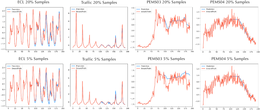
Figure 15: Visualization of input-$672$-predict-$96$ forecasting results of Timer trained with $5\%$ and $20\%$ samples.

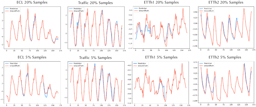
Figure 16: Visualization of imputation results of Timer trained with $5\%$ and $20\%$ samples.

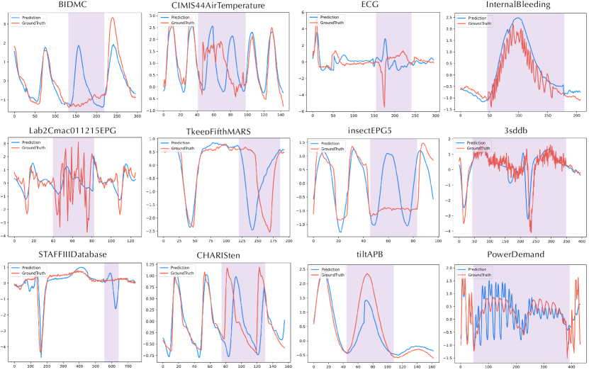
Figure 17: Visualization of anomaly detection results of Timer on partial UCR Anomaly Archive (Wu & Keogh, 2021). The masked part represents the abnormal position, and the model locates the abnormal interval by generating results that deviate from the abnormal series.

References

- Bai et al. (2018) Bai, S., Kolter, J. Z., and Koltun, V. An empirical evaluation of generic convolutional and recurrent networks for sequence modeling. arXiv preprint arXiv:1803.01271, 2018.
- Bao et al. (2021) Bao, H., Dong, L., Piao, S., and Wei, F. Beit: Bert pre-training of image transformers. arXiv preprint arXiv:2106.08254, 2021.
- Bengio et al. (2000) Bengio, Y., Ducharme, R., and Vincent, P. A neural probabilistic language model. Advances in neural information processing systems, 13, 2000.
- Bommasani et al. (2021) Bommasani, R., Hudson, D. A., Adeli, E., Altman, R., Arora, S., von Arx, S., Bernstein, M. S., Bohg, J., Bosselut, A., Brunskill, E., et al. On the opportunities and risks of foundation models. arXiv preprint arXiv:2108.07258, 2021.
- Box (2013) Box, G. Box and jenkins: time series analysis, forecasting and control. In A Very British Affair: Six Britons and the Development of Time Series Analysis During the 20th Century, pp. 161–215. Springer, 2013.
- Box et al. (2015) Box, G. E., Jenkins, G. M., Reinsel, G. C., and Ljung, G. M. Time series analysis: forecasting and control. John Wiley & Sons, 2015.
- Breunig et al. (2000) Breunig, M. M., Kriegel, H.-P., Ng, R. T., and Sander, J. Lof: identifying density-based local outliers. In Proceedings of the 2000 ACM SIGMOD international conference on Management of data, pp. 93–104, 2000.
- Chang et al. (2023) Chang, C., Peng, W.-C., and Chen, T.-F. Llm4ts: Two-stage fine-tuning for time-series forecasting with pre-trained llms. arXiv preprint arXiv:2308.08469, 2023.
- Chen et al. (2020) Chen, T., Kornblith, S., Norouzi, M., and Hinton, G. A simple framework for contrastive learning of visual representations. In International conference on machine learning, pp. 1597–1607. PMLR, 2020.
- Dai et al. (2022) Dai, D., Sun, Y., Dong, L., Hao, Y., Sui, Z., and Wei, F. Why can gpt learn in-context? language models secretly perform gradient descent as meta optimizers. arXiv preprint arXiv:2212.10559, 2022.
- Das et al. (2023a) Das, A., Kong, W., Leach, A., Sen, R., and Yu, R. Long-term forecasting with tide: Time-series dense encoder. arXiv preprint arXiv:2304.08424, 2023a.
- Das et al. (2023b) Das, A., Kong, W., Sen, R., and Zhou, Y. A decoder-only foundation model for time-series forecasting. arXiv preprint arXiv:2310.10688, 2023b.
- Dau et al. (2019) Dau, H. A., Bagnall, A., Kamgar, K., Yeh, C.-C. M., Zhu, Y., Gharghabi, S., Ratanamahatana, C. A., and Keogh, E. The ucr time series archive. IEEE/CAA Journal of Automatica Sinica, 6(6):1293–1305, 2019.
- Devlin et al. (2018) Devlin, J., Chang, M.-W., Lee, K., and Toutanova, K. Bert: Pre-training of deep bidirectional transformers for language understanding. arXiv preprint arXiv:1810.04805, 2018.
- Dong et al. (2023) Dong, J., Wu, H., Zhang, H., Zhang, L., Wang, J., and Long, M. Simmtm: A simple pre-training framework for masked time-series modeling. arXiv preprint arXiv:2302.00861, 2023.
- Dooley et al. (2023) Dooley, S., Khurana, G. S., Mohapatra, C., Naidu, S., and White, C. Forecastpfn: Synthetically-trained zero-shot forecasting. arXiv preprint arXiv:2311.01933, 2023.
- Elliott et al. (1996) Elliott, G., Rothenberg, T. J., and Stock, J. H. Efficient tests for an autoregressive unit root. Econometrica, 1996.
- Friedman (1962) Friedman, M. The interpolation of time series by related series. Journal of the American Statistical Association, 57(300):729–757, 1962.
- Godahewa et al. (2021) Godahewa, R., Bergmeir, C., Webb, G. I., Hyndman, R. J., and Montero-Manso, P. Monash time series forecasting archive. arXiv preprint arXiv:2105.06643, 2021.
- Goerg (2013) Goerg, G. Forecastable component analysis. In International conference on machine learning, pp. 64–72. PMLR, 2013.
- Hochreiter & Schmidhuber (1997) Hochreiter, S. and Schmidhuber, J. Long short-term memory. Neural computation, 9(8):1735–1780, 1997.
- Jin et al. (2023) Jin, M., Wang, S., Ma, L., Chu, Z., Zhang, J. Y., Shi, X., Chen, P.-Y., Liang, Y., Li, Y.-F., Pan, S., et al. Time-llm: Time series forecasting by reprogramming large language models. arXiv preprint arXiv:2310.01728, 2023.
- Kaplan et al. (2020) Kaplan, J., McCandlish, S., Henighan, T., Brown, T. B., Chess, B., Child, R., Gray, S., Radford, A., Wu, J., and Amodei, D. Scaling laws for neural language models. arXiv preprint arXiv:2001.08361, 2020.
- Kingma & Ba (2015) Kingma, D. P. and Ba, J. Adam: A method for stochastic optimization. In ICLR, 2015. URL http://arxiv.org/abs/1412.6980.
- Liu et al. (2022) Liu, M., Zeng, A., Chen, M., Xu, Z., Lai, Q., Ma, L., and Xu, Q. Scinet: time series modeling and forecasting with sample convolution and interaction. NeurIPS, 2022.
- Liu et al. (2023) Liu, Y., Hu, T., Zhang, H., Wu, H., Wang, S., Ma, L., and Long, M. itransformer: Inverted transformers are effective for time series forecasting. arXiv preprint arXiv:2310.06625, 2023.
- Muñoz-Sabater et al. (2021) Muñoz-Sabater, J., Dutra, E., Agustí-Panareda, A., Albergel, C., Arduini, G., Balsamo, G., Boussetta, S., Choulga, M., Harrigan, S., Hersbach, H., et al. Era5-land: A state-of-the-art global reanalysis dataset for land applications. Earth system science data, 13(9):4349–4383, 2021.
- Nie et al. (2022) Nie, Y., Nguyen, N. H., Sinthong, P., and Kalagnanam, J. A time series is worth 64 words: Long-term forecasting with transformers. arXiv preprint arXiv:2211.14730, 2022.
- OpenAI (2023) OpenAI, R. Gpt-4 technical report. arxiv 2303.08774. View in Article, 2:13, 2023.
- Paszke et al. (2019) Paszke, A., Gross, S., Massa, F., Lerer, A., Bradbury, J., Chanan, G., Killeen, T., Lin, Z., Gimelshein, N., Antiga, L., Desmaison, A., Köpf, A., Yang, E., DeVito, Z., Raison, M., Tejani, A., Chilamkurthy, S., Steiner, B., Fang, L., Bai, J., and Chintala, S. Pytorch: An imperative style, high-performance deep learning library. In NeurIPS, 2019.
- Radford et al. (2018) Radford, A., Narasimhan, K., Salimans, T., Sutskever, I., et al. Improving language understanding by generative pre-training. 2018.
- Radford et al. (2019) Radford, A., Wu, J., Child, R., Luan, D., Amodei, D., Sutskever, I., et al. Language models are unsupervised multitask learners. OpenAI blog, 1(8):9, 2019.
- Radford et al. (2021) Radford, A., Kim, J. W., Hallacy, C., Ramesh, A., Goh, G., Agarwal, S., Sastry, G., Askell, A., Mishkin, P., Clark, J., et al. Learning transferable visual models from natural language supervision. In International conference on machine learning, pp. 8748–8763. PMLR, 2021.
- Raffel et al. (2020) Raffel, C., Shazeer, N., Roberts, A., Lee, K., Narang, S., Matena, M., Zhou, Y., Li, W., and Liu, P. J. Exploring the limits of transfer learning with a unified text-to-text transformer. The Journal of Machine Learning Research, 21(1):5485–5551, 2020.
- Rasul et al. (2023) Rasul, K., Ashok, A., Williams, A. R., Khorasani, A., Adamopoulos, G., Bhagwatkar, R., Biloš, M., Ghonia, H., Hassen, N. V., Schneider, A., et al. Lag-llama: Towards foundation models for time series forecasting. arXiv preprint arXiv:2310.08278, 2023.
- Tan et al. (2021) Tan, C. W., Bergmeir, C., Petitjean, F., and Webb, G. I. Time series extrinsic regression: Predicting numeric values from time series data. Data Mining and Knowledge Discovery, 35:1032–1060, 2021.
- Touvron et al. (2023) Touvron, H., Lavril, T., Izacard, G., Martinet, X., Lachaux, M.-A., Lacroix, T., Rozière, B., Goyal, N., Hambro, E., Azhar, F., et al. Llama: Open and efficient foundation language models. arXiv preprint arXiv:2302.13971, 2023.
- Vaswani et al. (2017) Vaswani, A., Shazeer, N., Parmar, N., Uszkoreit, J., Jones, L., Gomez, A. N., Kaiser, Ł., and Polosukhin, I. Attention is all you need. Advances in neural information processing systems, 30, 2017.
- Wang et al. (2022a) Wang, T., Roberts, A., Hesslow, D., Le Scao, T., Chung, H. W., Beltagy, I., Launay, J., and Raffel, C. What language model architecture and pretraining objective works best for zero-shot generalization? In International Conference on Machine Learning, pp. 22964–22984. PMLR, 2022a.
- Wang et al. (2023) Wang, Y., Han, Y., Wang, H., and Zhang, X. Contrast everything: A hierarchical contrastive framework for medical time-series. arXiv preprint arXiv:2310.14017, 2023.
- Wang et al. (2022b) Wang, Z., Xu, X., Zhang, W., Trajcevski, G., Zhong, T., and Zhou, F. Learning latent seasonal-trend representations for time series forecasting. Advances in Neural Information Processing Systems, 35:38775–38787, 2022b.
- Woo et al. (2022) Woo, G., Liu, C., Sahoo, D., Kumar, A., and Hoi, S. Cost: Contrastive learning of disentangled seasonal-trend representations for time series forecasting. arXiv preprint arXiv:2202.01575, 2022.
- Woo et al. (2023) Woo, G., Liu, C., Kumar, A., and Sahoo, D. Pushing the limits of pre-training for time series forecasting in the cloudops domain. arXiv preprint arXiv:2310.05063, 2023.
- Wu et al. (2021) Wu, H., Xu, J., Wang, J., and Long, M. Autoformer: Decomposition transformers with auto-correlation for long-term series forecasting. Advances in Neural Information Processing Systems, 34:22419–22430, 2021.
- Wu et al. (2022) Wu, H., Hu, T., Liu, Y., Zhou, H., Wang, J., and Long, M. Timesnet: Temporal 2d-variation modeling for general time series analysis. arXiv preprint arXiv:2210.02186, 2022.
- Wu & Keogh (2021) Wu, R. and Keogh, E. Current time series anomaly detection benchmarks are flawed and are creating the illusion of progress. IEEE Transactions on Knowledge and Data Engineering, 2021.
- Xu et al. (2021) Xu, J., Wu, H., Wang, J., and Long, M. Anomaly transformer: Time series anomaly detection with association discrepancy. arXiv preprint arXiv:2110.02642, 2021.
- Yan et al. (2021) Yan, W., Zhang, Y., Abbeel, P., and Srinivas, A. Videogpt: Video generation using vq-vae and transformers. arXiv preprint arXiv:2104.10157, 2021.
- Yue et al. (2022) Yue, Z., Wang, Y., Duan, J., Yang, T., Huang, C., Tong, Y., and Xu, B. Ts2vec: Towards universal representation of time series. In Proceedings of the AAAI Conference on Artificial Intelligence, volume 36, pp. 8980–8987, 2022.
- Zeng et al. (2023) Zeng, A., Chen, M., Zhang, L., and Xu, Q. Are transformers effective for time series forecasting? In Proceedings of the AAAI conference on artificial intelligence, volume 37, pp. 11121–11128, 2023.
- Zerveas et al. (2021) Zerveas, G., Jayaraman, S., Patel, D., Bhamidipaty, A., and Eickhoff, C. A transformer-based framework for multivariate time series representation learning. In Proceedings of the 27th ACM SIGKDD conference on knowledge discovery & data mining, pp. 2114–2124, 2021.
- Zhang et al. (2022) Zhang, X., Zhao, Z., Tsiligkaridis, T., and Zitnik, M. Self-supervised contrastive pre-training for time series via time-frequency consistency. Advances in Neural Information Processing Systems, 35:3988–4003, 2022.
- Zhao et al. (2023) Zhao, W. X., Zhou, K., Li, J., Tang, T., Wang, X., Hou, Y., Min, Y., Zhang, B., Zhang, J., Dong, Z., et al. A survey of large language models. arXiv preprint arXiv:2303.18223, 2023.
- Zhou et al. (2021) Zhou, H., Zhang, S., Peng, J., Zhang, S., Li, J., Xiong, H., and Zhang, W. Informer: Beyond efficient transformer for long sequence time-series forecasting. In Proceedings of the AAAI conference on artificial intelligence, volume 35, pp. 11106–11115, 2021.
- Zhou et al. (2023) Zhou, T., Niu, P., Wang, X., Sun, L., and Jin, R. One fits all: Power general time series analysis by pretrained lm. arXiv preprint arXiv:2302.11939, 2023.