Exploring Intrinsic Properties of Medical Images for
Self-Supervised Binary Semantic Segmentation

Abstract

Recent advancements in self-supervised learning have unlocked the potential to harness unlabeled data for auxiliary tasks, facilitating the learning of beneficial priors. This has been particularly advantageous in fields like medical image analysis, where labeled data are scarce. Although effective for classification tasks, this methodology has shown limitations in more complex applications, such as medical image segmentation. In this paper, we introduce Medical imaging Enhanced with Dynamic Self-Adaptive Semantic Segmentation (MedSASS), a dedicated self-supervised framework tailored for medical image segmentation. We evaluate MedSASS against existing state-of-the-art methods across four diverse medical datasets, showcasing its superiority. MedSASS outperforms existing CNN-based self-supervised methods by 3.83% and matches the performance of ViT-based methods. Furthermore, when MedSASS is trained end-to-end, covering both encoder and decoder, it demonstrates significant improvements of 14.4% for CNNs and 6% for ViT-based architectures compared to existing state-of-the-art self-supervised strategies.

¹Center for Data Science, New York University, New York, USA
²Department of Computer Science, Courant Institute of Mathematical Sciences, New York University, New York, USA
³Colton Center for Autoimmunity, NYU Grossman School of Medicine, New York, USA

1 Introduction

The field of medical image analysis represents a significant application of deep learning, typically involving tasks such as classification and segmentation. Classification entails categorizing each image into one or more classes. In contrast, segmentation, a more intricate task, requires categorizing each pixel in an image. Among these, semantic segmentation, which involves differentiating the image into foreground and background, is particularly crucial in medical imaging. This process is essential for isolating objects of interest (e.g., lesions in skin lesion imaging or cells in histopathology slides) from irrelevant areas, aiding clinicians in making more informed decisions.

Artificial intelligence has markedly enhanced the effectiveness of medical image analysis tools. A key principle in this domain is that AI-driven methods enhance performance proportionally to the volume of labeled data used in training. However, acquiring medical imaging data can be costly, time-consuming, and subject to varying levels of bureaucratic approval, posing challenges to the release of large-scale, well-labeled datasets. Recently, improvements in self-supervised learning methods have made it possible to use unlabeled data to learn priors, which can then be used to improve the performance of downstream tasks. During pre-training self-supervised techniques, perform an auxiliary task on unlabeled data to learn priors. Existing state-of-the-art self-supervised approaches only focus on training an encoder. While this approach works well for classification, where we only need an encoder, in the case of more intricate tasks like segmentation, we need an encoder-decoder pair. Additionally, it has been shown that only improving the encoder is effective to an extent and that to make further gains, improving the decoder is needed (Singh et al., 2023).

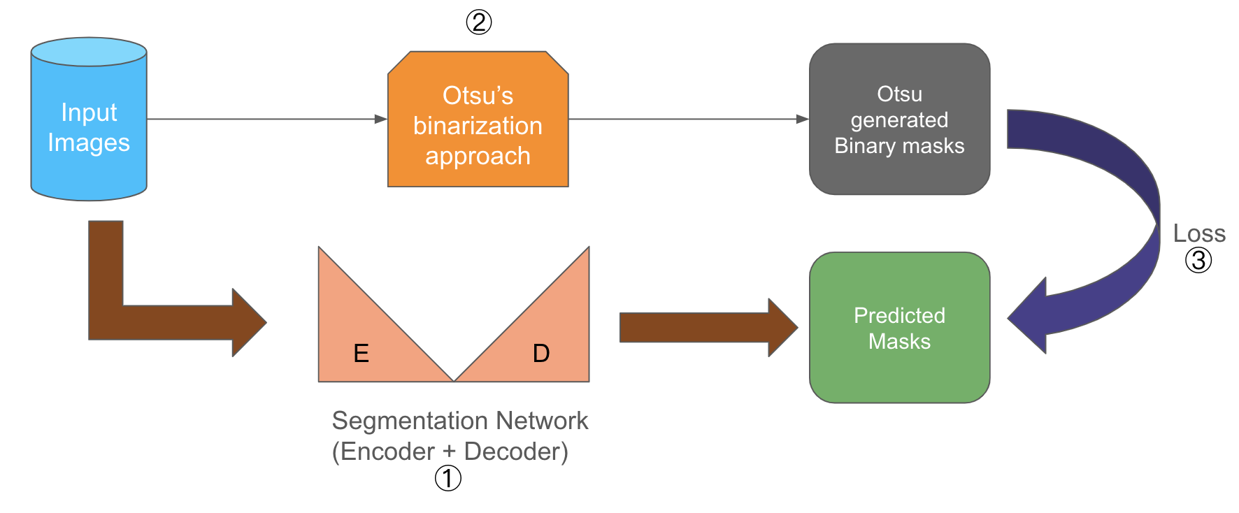
Figure 1: In this figure, we depict the pre-training procedure of MedSASS. Our input is only images; during each iteration, the input images are simultaneously passed through the segmentation network and Otsu’s approach (Otsu, 1979). The output labels of these two are used to compute loss and optimize the segmentation network. We ablate the three fundamental components of MedSASS: the segmentation architecture (\raisebox{-.9pt} {1}⃝), the thresholding approach for self-supervision (\raisebox{-.9pt} {2}⃝), and the loss function (\raisebox{-.9pt} {3}⃝) in Sections 4.2 , 5.1 and 5.2 respectively.

To better align self-supervised learning with the demands of semantic segmentation, we introduce a novel methodology: MedSASS (Medical Imaging Enhanced with Dynamic Self-Adaptive Semantic Segmentation). We begin with an overview of existing self-supervised techniques in Section 2, then delve into the conceptual underpinnings of MedSASS in Section 3. Section 4 outlines our experimental setup and compares MedSASS’s performance against existing self-supervised methods in semantic segmentation. This comparison encompasses four medical imaging datasets of varying sizes and modalities, employing both CNN and ViT backbones.

• We propose a novel self-supervised technique for medical image segmentation, Medical imaging Enhanced with Dynamic Self-Adaptive Semantic Segmentation (MedSASS). This technique improves over existing state-of-the-art self-supervised techniques by 3.83% for CNNs and on-par for ViT-based semantic segmentation architecture over four diverse medical image segmentation datasets with encoder-only training.

• Additionally, unlike existing self-supervised techniques that only train an encoder, with MedSASS we can train end-to-end (an encoder as well as a decoder). With this approach, MedSASS improves segmentation performance (IoU metric) by 14.4% for CNNs and 6% for ViT over existing self-supervised techniques.

• To the best of our knowledge, this is the first large-scale study covering multiple self-supervised techniques for CNNs and Vision Transformers on four challenging medical datasets.

2 Related Work

Recent developments in self-supervised learning literature predominantly feature two main pre-training approaches: (i) the use of contrastive loss, and (ii) masked image modeling. Contrastive loss-based methods focus on learning through the matching of similarities and dissimilarities. Traditionally, such techniques have optimized distances between representations of different augmented views of the same image (referred to as ‘positive pairs’) and those from different images (‘negative pairs’), as demonstrated by (He et al., 2020; Chen et al., 2020; Caron et al., 2020). However, this approach is memory-intensive, necessitating the tracking of both positive and negative pairs. Recent state-of-the-art approaches like Bootstrap Your Own Latent (BYOL) (Grill et al., 2020) and Distillation with NO labels (DINO) (Caron et al., 2021) have enhanced this performance by omitting the need for memory banks. The use of negative pairs in these models serves to prevent collapse, a challenge that has been tackled through various strategies. BYOL employs a momentum coder, while Simple Siamese (SimSiam) (Chen & He, 2021) utilizes a stop gradient. DINO, on the other hand, employs a combination of sharpening and centering to counterbalance and avoid collapse. Techniques that rely solely on positive pairs have proven to be more efficient than those requiring both positive and negative pairs. At the same time, there has been a rise in reconstruction-based, self-supervised pre-training methods like SimMIM (Xie et al., 2022) and MAE (He et al., 2022). These methods aim to comprehend the semantic aspects of images by masking certain sections and subsequently predicting these masked portions during pre-training.

Notably, current self-supervised techniques primarily train only an encoder. Yet, for effective segmentation, both an encoder and a decoder equipped with robust priors are essential. While reconstructive self-supervised methods (like SimMIM (Xie et al., 2022) and MAE (He et al., 2022)) do involve a decoder during pre-training, they are not directly applicable for segmentation tasks. For instance, SimMIM employs a linear layer decoder, which is considerably simpler than a U-Net (Ronneberger et al., 2015) decoder and focuses solely on predicting the masked portion. Concurrently, the concept of training an encoder-decoder architecture end-to-end has been investigated in fields like self-supervised depth estimation (Godard et al., 2019). While the efficacy of existing state-of-the-art self-supervised methods has been extensively examined in the realm of natural imaging, only a limited number of studies have delved into their application in medical image segmentation. Those that do include self-supervised medical image segmentation typically have a constrained scope, with a limited range of approaches and techniques explored, as indicated in (Kalapos & Gyires-Tóth, 2022).

To the best of our knowledge, there are no comprehensive studies that extensively explore self-supervised medical image segmentation across various medical modalities. Moreover, there is a lack of investigation into the impacts of pre-training both the encoder and decoder within the context of self-supervised medical image segmentation.

3 Description of MedSASS

3.1 Intuition for MedSASS

MedSASS incorporates a semantic segmentation architecture: U-Net, selected for its preeminence in biomedical image segmentation (Ronneberger et al., 2015). To facilitate self-supervised training, we use the input image and obtain a prediction using Otsu’s approach (Otsu, 1979). The objective of the self-supervised training is to predict the Otsu’s output. Since we get semantic segmentation masks from Otsu’s approach, we can train either an encoder or an end-to-end architecture. The choice of Otsu’s method capitalizes on the intrinsic properties of input images as supervisory signals, embodying the essence of self-supervised learning.

As previously highlighted, acquiring labels for medical images is both costly and time-consuming. However, these labels are essential for developing advanced image analysis techniques. In the realm of medical image analysis, semantic segmentation stands out as particularly complex yet common task. One strategy to circumvent this challenge is through self-supervised approaches. As mentioned in Section 2, traditional self-supervised methods involve auxiliary tasks during pre-training, such as clustering, self-distillation, or masked image modeling. These tasks typically involve training an encoder for a specific task, followed by fine-tuning for subsequent tasks like classification or segmentation. For classification, this method is straightforward, but for segmentation, it only pre-trains a portion of the architecture, typically the encoder. Segmentation architectures usually comprise both an encoder and a decoder. Existing self-supervised techniques pre-train only the encoder, thus providing partial support to these architectures. MedSASS advances this by pre-training both the encoder and decoder, unlocking greater performance potential. Unlike most existing self-supervised pre-training objectives, which lean towards classification, MedSASS is designed with a segmentation-centric objective. It involves training a U-Net architecture (Ronneberger et al., 2015) to predict binarized masks, as mentioned in Section 3. We utilize input images (minus their ground truth) and leverage Otsu’s technique for self-supervision, as depicted in Fig. 2. A loss function is then computed against the Otsu-computed masks and the output from the segmentation architecture (denoted by \raisebox{-.9pt} {1}⃝ in Fig. 1). We use a combination of distribution and region-based loss functions in MedSASS and discuss this with empirical results in Section 5.2. As our method depends solely on input images without labels, it remains self-supervised. Initially, we pre-train only the encoder part of the U-Net for a fair comparison with existing methods. In this phase, MedSASS demonstrated a performance enhancement of 3.83% over state-of-the-art self-supervised approaches for CNNs and was on average par with the performance with ViT, measured across four medical imaging datasets using the IoU metric. When incorporating the pre-trained encoder with the decoder, we observed an even more significant performance leap: a 14.4% gain for CNNs and 6% for ViT compared to existing self-supervised approaches.

3.2 Why Otsu’s (Otsu, 1979) approach ?

Self-Supervised Technqiue	Backbone	Dataset
		Dermatomyositis	TissueNet	ISIC-2017	X-Ray
DINO	ResNet-50	0.1399 ±0.056	0.2972 ±0.129	0.2426±0.0027	0.2052 ±0.0899
BYOL	ResNet-50	0.1278 ±0.072	0.2939 ±0.124	0.2412 ±0.0022	0.2185 ±0.00834
SimSiam	ResNet-50	0.1415 ±0.0548	0.3021 ±0.143	0.2395 ±0.0198	0.1939 ±0.11
MedSASS (e)	ResNet-50	0.1742 ±0.0481	0.3824 ±0.00579	0.2445 ±0.00482	0.2568 ±0.0161

Table 1: The table showcases the Intersection over Union (IoU) scores averaged across five distinct seed values for a U-Net architecture equipped with a ResNet-50 backbone, tested across four diverse medical imaging datasets. To highlight the superior performance, the top-performing numbers are emphasized in bold, while the second-best results are underscored with an underline for each dataset. MedSASS (e) is indicative of our focus on training only the encoder of MedSASS, aligning with the training scope of other self-supervised techniques for a balanced comparison. Notably, MedSASS demonstrates superior performance over other leading self-supervised methods across all datasets, employing a ResNet-50 backbone. This observation underscores the effectiveness of MedSASS in enhancing the capabilities of self-supervised learning in medical image analysis.

MedSASS aims to pioneer a self-supervised approach for medical semantic segmentation. Typically,semantic segmentation in medical imaging entails differentiating the area of interest (foreground) from the non-relevant area (background). For instance, in skin lesion imaging, the task involves isolating the lesion (foreground) from the rest of the dermatology slide, and similarly, in histopathology slides, distinguishing cells (foreground) from the slide background. Consequently, this necessitates binary masks.

In MedSASS, we employ Otsu’s approach, a classic technique widely used in medical imaging, for semantic segmentation to this day on datasets that are too small to train using deep neural networks (Barron, 2020). During pre-training the architecture is trained to predict masks generated by Otsu’s approach. There are certain priors associated with medical imaging that make the application of Otsu’s approach favorable in medical images as compared to natural images. In this section we provide the rationale for using Otsu’s approach, followed by empirical results in Section 4.2 and qualitative samples in Appendix F. These priors include:

• In medical imaging, high contrast is ensured to best visualize disease features. Otsu’s approach effectively separates high-contrast areas, making it ideal for medical images (Dance et al., 2014).

• Medical images typically have a more straightforward and consistent background-foreground relationship. For instance, in an X-ray, the bones might be the foreground, and everything else is the background. Otsu’s approach, which works by finding a threshold that best separates these two classes, is well-suited for such scenarios. Natural images, however, often contain multiple objects, textures, and gradients, making it difficult for a single threshold to effectively segment all relevant objects as elucidated in Appendix E. In medical imaging, the primary goal of segmentation is often to isolate specific anatomical structures or pathologies, which are usually distinct in intensity from the surrounding tissue. Otsu’s approach efficiently accomplishes this by focusing on the intensity differences. In natural imaging, segmentation goals are more diverse and may require identifying and separating multiple objects and textures, which necessitates more sophisticated segmentation techniques. We further empirically validate these in Appendix E where we observe that MedSASS with Otsu’s approach performs sub-par as compared to other self-supervised techniques.

• Medical imaging techniques are usually conducted in controlled environments with uniform lighting, which leads to more consistent image quality. This consistency is conducive to the application of Otsu’s technique, which assumes a bimodal histogram (two distinct peaks representing the foreground and background). On the other hand, natural images are taken under varying lighting conditions and may not exhibit a clear bimodal histogram, reducing the effectiveness of Otsu’s approach (Pham et al., 2000).

Traditionally, and to this day, Otsu’s method is used for segmentation in the medical imaging community for datasets that are too small to train on (Barron, 2020). Furthermore, Otsu’s masks have been used for comparison against neural networks. To the best of our knowledge, MedSASS is the first approach to leverage this ”automatic” approach for self-supervision (Kumar et al., 2017). In our methodology, we first convert images to grayscale and then apply Otsu’s technique to generate thresholded masks. Otsu’s technique dynamically calculates the threshold for each image, enabling the segmentation architecture to learn meaningful representations rather than adapting to a specific threshold value. We also juxtapose MedSASS’s performance using other ”automatic” methods for obtaining binarized masks, such as adaptive thresholding Chan et al. (1998) and Generalized Histogram Thresholding (GHT) (Barron, 2020), to underscore the efficacy of Otsu’s approach in diverse imaging scenarios in Section 5.1.

How MedSASS avoids collapse ?

In MedSASS, we avoid collapsing (i) by making sure the architecture is not focusing on trivial learning and is actually learning useful priors. (ii) By making sure the architecture is learning equally, focusing on the majority and the minority class. We start by explaining how we are preventing the creation of trivial masks, as they are used for supervision. Followed by a rationale for balanced learning.

Otsu’s (Otsu, 1979) approach has been reliably used for segmentation of medical imaging on datasets that are too small to train on (Barron, 2020). Although these labels are not exactly as good as ground truth labels, they still help the architecture to learn useful priors. Additionally, Otsu’s approach suffers in the case of complex images, but in our experiments, we observed that even though Otsu provides subpar supervision for a few samples, across the dataset, it is a good supervisor. We prevent some examples of the labels generated by Otsu’s approach in Appendix F and empirical results in Section 4.2. In dimensional collapse, a particular architecture starts clubbing all/most of the latent variables into the same representation. This could have been a possibility in the case of obtaining labels for supervision by randomly setting a pixel threshold value throughout the dataset. In Otsu’s approach, each image has a different threshold value determined by minimizing intra-class intensity variance, or equivalently, by maximizing inter-class variance. Thus, a pixel with the same pixel intensity can be classified as background or foreground based on its context, as opposed to the case when we simply set a threshold and all values are clustered based on their values, irrespective of the context. Setting a fixed threshold $x$ in image segmentation implies that all pixel values below $x$ are classified as background (bg) across the entire dataset, regardless of their context. This results in their representations converging to a singular point in the latent space. However, in Otsu’s approach, the threshold is not constant but varies from one image to another. Consequently, while pixels below a certain value $x_{1}$ might be classified as background in one image, they could be deemed foreground (fg) in another image within the same dataset. This variability compels the architecture to genuinely learn and discern useful image features, enhancing its ability to make accurate prior predictions and avoid dimensional collapse. We further investigated a variety of thresholding approaches in Section 5.1.

But even with this non-trivial thresholding, there is a possibility that the image is split into an imbalanced number of foreground and background pixels. And during training, the architecture overfits to one of them. This does happen when we use cross-entropy loss, as elucidated in (Lin et al., 2017; Singh et al., 2023) and Section 2. To prevent this from happening, we use a combination of distribution and region-based loss functions, as explained in Section 2.

4 Experimental Setup and Results

Although Otsu’s masks are not accurate for a lot of the images, particularly for complex images. Our rationale is to learn representations by predicting Otsu’s label during pre-training. Furthermore, traditionally, Otsu’s label have been found to be effectively segment medical images (Barron, 2020). We provide samples of masks generated by Otsu’s approach, along with sample images for all datasets used for experimentation in Appendix F. Our experimental approach aligns with the methodologies of Caron et al. (2021) and Jabri et al. (2020), focusing exclusively on k-mean features for segmentation. MedSASS offers two distinct training methodologies: (i) encoder only training, and (ii) end-to-end training. We have conducted a thorough pre-training of all self-supervised models for 50 epochs, utilizing a batch size of 16 and early stopping patience of five epochs. Our evaluation includes the Intersection over Union (IoU) scores on the test set, averaged over five different seed values across four distinct medical imaging datasets of varying modalities. The results are methodically presented, beginning with the outcomes of training solely the encoder in Section 4.2.1, for fair comparison with existing state-of-the-art self-supervised techniques. Followed by the results from training both the encoder and decoder in Section 4.2.2. In addition to this we provide additionally results such as comparison with Supervised approaches in Appendix C, training with different batch size and pre-training epochs in Appendix B.2 and performance on other vision tasks like classification in Appendix D. We provide additional implementation details in Appendix A.

Dataset	IoU on Test Set
	Tversky Loss	Focal Loss	Focal Tversky
Derm.	0.1726 ±0.000133	0.02 ±0.0181	0.181 ±0.0068
ISIC-2017	0.2444 ±0.00597	0.05291 ±0.0907	0.4847 ±0.0277
TN.	0.3604 ±0.0301	0.11 ±0.0117	0.5077 ±0.0103
X-Ray	0.1963 ±0.113	0.02 ±0.0261	0.3522 ±0.00238

Table 2: This table presents a comparative analysis of MedSASS trained using various loss functions: tversky loss, focal loss, and focal-tversky loss. Additionally, we also studied the effect of using cross-entropy loss in Appendix B.1. In the case of cross-entropy loss, we note a collapse in the model’s performance. Further, our observations highlight that focal-tversky loss significantly outperforms the models trained with either focal or Tversky loss alone.

Self-Supervised Technique	Backbone	Dataset
		Dermatomyositis	TissueNet	ISIC-2017	X-Ray
DINO	ViT-small	0.1668 ±0.00987	0.2483 ±0.143	0.1891±0.0031	0.2106±0.0651
MAE	ViT-small	0.1668 ±0.00996	0.3455 ±0.08	0.191±0.0819	0.2106 ±0.0649
SimMIM	ViT-small	0.167 ±0.00993	0.3335 ±0.0867	0.1913±0.072	0.2077±0.00247
MedSASS (e)	ViT-small	0.136 ±0.0793	0.3633 ±0.00624	0.1914 ±0.0839	0.2466 ±0.00302

Table 3: In this table, we present the results of U-Net trained with ViT-small backbone on four diverse medical imaging datasets over five different seed values. Numbers mentioned in bold is the best performing while numbers mentioned with an underline is the next best performing. Additionally, MedSASS (e) represents that we are only training the encoder of MedSASS, for fair comparison with other self-supervised techniques. We observe that MedSASS outperforms existing state-of-the-art self-supervised approaches for three out of the four datasets with a ViT-small backbone. Furthermore, we observe that masked image modeling-based self-supervised techniques like MAE and SimMIM perform better than contrastive self-distilling approaches like DINO.

4.1 Datasets

The Dermatomyositis dataset

(Singh & Cirrone, 2023; Van Buren et al., 2022) This dataset is made up of whole-slide images that were cut from muscle biopsies of patients with Dermatomyositis, stained with different proteins, and then imaged to make a dataset of 198 TIFF images from 7 patients. We use the DAPI-stained images for the semantic segmentation, in line with previous works (Singh & Cirrone, 2023; Van Buren et al., 2022). Each whole slide image is 1408 by 1876. We tile these whole slide images into a size of $480\times 480$. We then split these datasets into a ratio of 70/10/20 for training, validation, and testing, respectively. This split yields 1656, 240, and 480 images in the training, validation, and test sets, respectively.

Tissuenet dataset

(Greenwald et al., 2022) This dataset contains over a million cells annotations from nine different organs, and six different imaging systems are annotated. Each cell has both nuclear and whole-cell information. Each image in the validation and test sets is $256\times 256$, while training images are $512\times 512$ in size. We use the official splits of the dataset for training, validation, and testing, with 2580, 3140, and 1249 images, respectively.

ISIC-2017 dataset

(Codella et al., 2017) The International Skin Imaging Collaboration (ISIC) 2017 image dataset is one of the largest repositories of images of melenoma skin lesions, the most lethal skin cancer. Each image has binary image masks of the lession region and background. The dataset is segmented into three parts: training, validation, and testing, with 2000, 150, and 600 images, respectively. The ISIC-2017 is a particularly hard dataset due to high intra-class variability and inter-class similarities with obscuration areas of interest (Singh et al., 2023).

X-ray image dataset

(Chowdhury et al., 2020; Rahman et al., 2021) This is the largest dataset used in our study, with a total of 21,165 images. We split the dataset into 14,730, 2202, and 4,233 images for training, validation, and testing, respectively. The X-ray dataset contains chest X-ray images of patients with COVID-19, normal, and other lung infections. Each image in the dataset is $299\times 299$.

Across all four datasets, our task is semantic segmentation, i.e., segmenting an area of interest (foreground) from the area of no interest (background). For evaluation on the test set, we use the IoU (Intersection over Union) score for comparison. Additionally, we further expand upon the challenges associated with each of these datasets along with samples in Appendix F.

4.2 Results

4.2.1 Encoder only training

Existing self-supervised techniques pre-train an encoder that can then be used on a variety of downstream tasks. We start by only training the encoder of MedSASS. During this encoder-only pre-training, we only keep the encoder and discard everything else. We then transfer the saved weights of this encoder to evaluate the testing set of each dataset. We don’t fine-tune and use the learned features for semantic mask prediction, similar to (Caron et al., 2021) and (Jabri et al., 2020). We present the results of this training procedure with a ResNet-50 backbone in Table 1 and with a ViT-small backbone in Table 3. We observed that MedSASS outperforms existing state-of-the-art self-supervised techniques with a CNN backbone, U-Net. For the ViT-small U-Net, we observed that MedSASS outperforms existing state-of-the-art self-supervised techniques on three (out of four) datasets and overall is on par with them.

4.2.2 Encoder with Decoder training

As mentioned already, existing state-of-the-art self-supervised techniques aim to pretrain an encoder and then use it for downstream tasks. For classification, this is pretty straightforward, as we only need to train a small MLP on top of the pre-trained encoder. But for segmentation, usually a more complex and much deeper decoder is used to predict the mask from the latent representation extracted from the pre-trained encoder. With MedSASS, we can pre-train a U-Net end-to-end for semantic segmentation in a self-supervised way. Instead of getting rid of everything except the encoder (as mentioned in encoder-only training in Section 4.2.1), for end-to-end training, train a reusable decoder that can then be used directly for segmentation. We provide a complete set of results comparing the end-to-end encoder-only and existing state-of-the-art pre-training performance of MedSASS for CNN in Figure 2 and in Figure 3 for ViT-small.

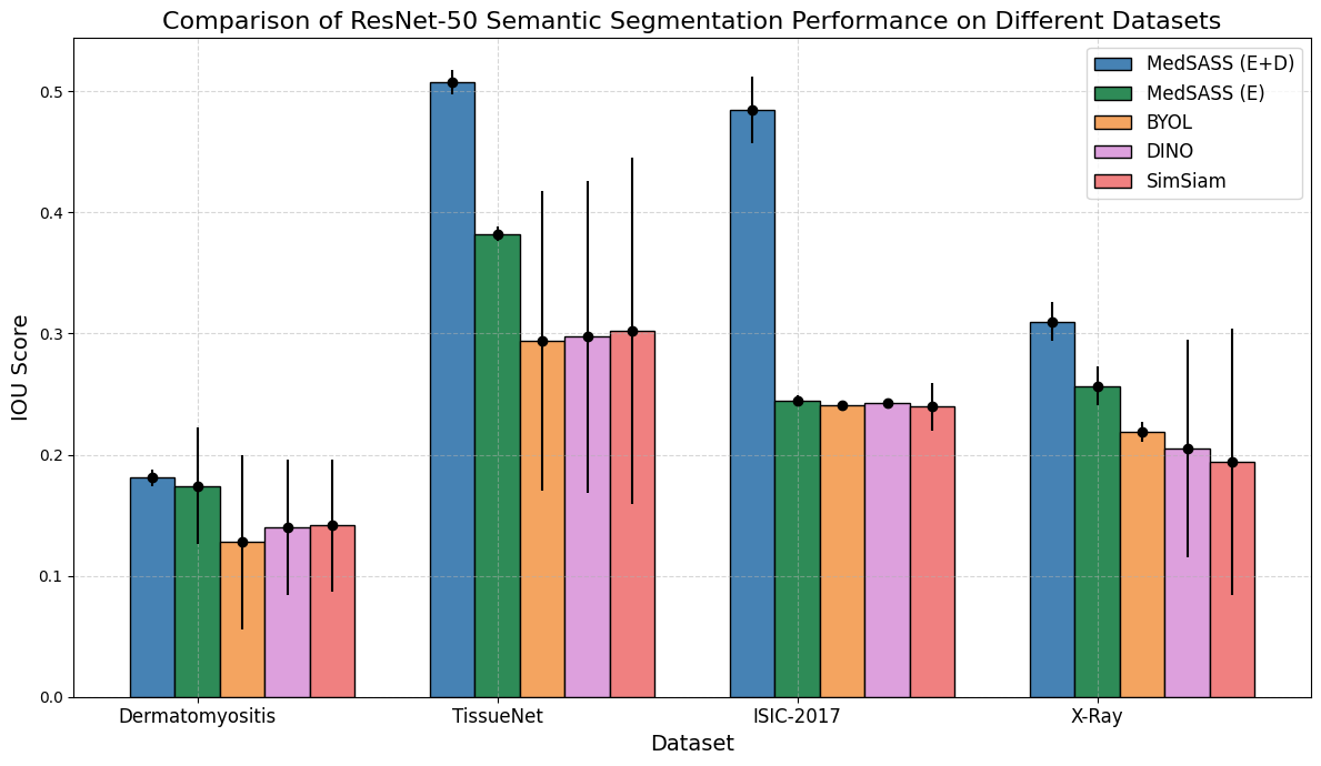
Figure 2: In this figure, we present a comparative analysis of various training methodologies: MedSASS with both encoder and decoder (denoted as MedSASS (E+D)), MedSASS utilizing only the encoder (denoted as MedSASS (E)), BYOL, DINO, and SimSiam. Our findings reveal that MedSASS, when trained solely with an encoder (indicated in green), surpasses all existing state-of-the-art self-supervised techniques in semantic segmentation performance. Moreover, the end-to-end training of MedSASS demonstrates an even more pronounced advantage over these state-of-the-art self-supervised approaches in the same domain. While the encoder only pre-trained MedSASS surpasses current state-of-the-art self-supervised methods by an average of 3.83%, averaged over four datasets and five different seeds per dataset. Remarkably, when MedSASS is pre-trained end-to-end, it outperforms these state-of-the-art self-supervised methods by an even more significant margin of 14.4%, also averaged over the same four datasets and seed settings. The black dot on top of each bar with horizontal line represent the error bar for average over five seed values.

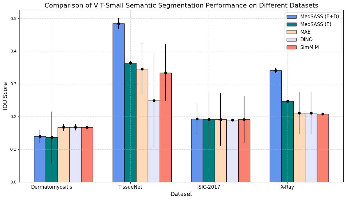
Figure 3: This bar graph illustrates a comparison between end-to-end and encoder-only pretrained MedSASS against other state-of-the-art self-supervised techniques, all utilizing a ViT-small backbone. We note that MedSASS, when solely pretrained, aligns closely in performance with other state-of-the-art self-supervised methods for semantic segmentation. Notably, MedSASS achieves an average improvement of 6% over these state-of-the-art techniques when trained end-to-end, as evidenced across the four datasets. Similar to Figure 2, black dot on top of each bar with horizontal line represent the error bar.

5 Ablation study

5.1 Change in Thresholding Technique

The efficacy of thresholded masks is crucial for MedSASS, as it depends on them for supervision. The simplest method to create these masks involves setting a fixed threshold value for supervision. However, this approach has a significant drawback: the model might not learn meaningful features but rather categorize pixels based solely on whether they fall above or below this threshold. This results in the architecture merely learning to threshold at the set value instead of acquiring useful features. Moreover, applying a uniform global threshold may not be effective, as different areas within an image could exhibit varying pixel intensities. In such cases, a global threshold might obscure details that are critical for the architecture to learn valuable representations. Furthermore, this could also lead to dimensional collapse, wherein instead of learning useful latent representation, they are compressed and clustered at a single point.

To address this challenge, adaptive thresholding can be employed. This technique adjusts the threshold for each pixel based on the surrounding region, providing variable thresholds for different image areas, which is advantageous in images with diverse pixel intensities. Nonetheless, adaptive thresholding methods also necessitate an initial arbitrary pixel value. To circumvent the need for a predefined threshold, techniques like Otsu’s approach (Otsu, 1979) can be utilized. Otsu’s approach dynamically calculates the threshold by minimizing intra-class intensity variance, or alternatively, maximizing inter-class variance. This strategy optimizes the threshold value for each individual image rather than applying a uniform value across the dataset. Otsu’s method, widely used in medical imaging and OCR, is particularly beneficial for small datasets that are challenging to train. Its popularity has led to the development of an improved and generalized version combinig Otsu’s method with minimum error thresholding (Kittler & Illingworth, 1986) into a Generalized Histogram Thresholding (Barron, 2020).

In this section, we explore the impact of different thresholding techniques. We start with two examples of adaptive thresholding (Chan et al., 1998) —mean and gaussian thresholding—followed by Otsu’s (Otsu, 1979) approach and the more advanced, generalized Generalized Histogram Thresholding (GHT) (Barron, 2020). We train a Resnet-50 (He et al., 2015) MedSASS end-to-end for 50 epochs with a batch size of 16 and report the IoU averaged over five seeds for four datasets in Table 4. Our findings indicate that while all techniques perform comparably on the Dermatomyositis dataset, they fall short of the performance achieved by Otsu’s approach-supervised MedSASS across datasets.

5.2 Change in Loss Function

As a default, we use focal-tversky loss in MedSASS. In this section, we start by providing a rationale for using focal-tversky loss, followed by empirical results to support our choice of function.

Why focal-tversky loss ?

Region- or distribution-based loss functions are commonly utilized in medical image segmentation. For instance, binary cross-entropy loss, a variant of cross-entropy loss, exemplifies a distribution-based loss function. However, it often tends to overfit the predominant class in binary image segmentation (Singh et al., 2023), which can be either the foreground or background. To address this issue, focal loss (Lin et al., 2017) was developed. It differentially weights the majority and minority classes, thereby preventing overfitting of the majority class through targeted penalization.

In contrast, DICE loss (Sudre et al., 2017), a region-based loss function, is adapted from the DICE coefficient used in evaluating segmentation performance. However, it equally treats False Positives (FP) and False Negatives (FN), which is a notable limitation in medical imaging. The impact of FPs and FNs in this field is asymmetric; for example, missing a pathological feature (FN) can be more detrimental than a false alarm (FP), as it could result in missed diagnoses and delayed treatments. To mitigate this, tversky loss (Salehi et al., 2017) was introduced, applying variable weights to the FP and FN classes. Our selection of focal-tversky (Abraham & Khan, 2019) loss is driven by its hybrid nature, combining elements of both distribution and region-based loss functions. This approach effectively prevents overfitting to a specific pixel class and provides a focused addressal for FNs, aligning more closely with the nuanced needs of medical image analysis. We present these results in Table 2. From this table, we observe that focal-tversky loss performs much better than focal and tversky loss.

Furthermore, we also provide ablation study of changing the number of pre-training epochs and batch size for MedSASS in Appendix B.2. From Table 5, we observed that both the CNN and ViT based MedSASS are robust to change in pre-training epoch. Similarly, for the change in batch size, from Tables 7 and 8, we observe that overall the performance remains constant except for a minute improvement when we switch to a batch size of 8.

Dataset	Adaptive Thresholding (Mean)	Adaptive Thresholding (Gaussian)	GHT (Barron, 2020)	Otsu (Otsu, 1979)
Dermatomyositis	0.1724±0.002	0.1725 ±0.004	0.1809 ±0.0227	0.181 ±0.0068
ISIC-2017	0.2393 ±0.001	0.2393 ±0.006	0.1236 ±0.0039	0.4847±0.0277
TissueNet	0.3949 ±0.0087	0.391 ±0.00899	0.4927 ±0.00885	0.5077 ±0.0103
X-Ray	0.1839 ±0.00189	0.2079 ±0.0048	0.1689 ±0.0281	0.3522 ±0.00238

Table 4: This table displays IoU scores for MedSASS using various thresholding methods: adaptive thresholding (Chan et al., 1998) (Mean and Gaussian), GHT (Barron, 2020), and Otsu’s approach (Otsu, 1979), across four datasets. The results are presented as IoU scores averaged over five seed values with standard deviations, showcasing the performance variation of each technique in medical image segmentation. We observe that overall Otsu’s approach provides the best supervision for MedSASS.

6 Discussion and Conclusion

Impact in Healthcare

Medical image analysis is one of the most pivotal and challenging domains for application of artificial intelligence. Its effectiveness hinges largely on the availability of high-quality and abundant training labels. However, acquiring these labels is costly and time-consuming. During crises, the challenge is exacerbated; clinicians and experts, who are essential for labeling images, are overwhelmingly occupied with patient care and triage. In these critical times, AI systems have the potential to alleviate the burden on clinicians through automated analysis. Self-supervised methods like MedSASS are particularly valuable in addressing this dilemma. Due to their self-supervised nature they can be scaled without labels. This attribute is especially beneficial in scenarios like region-specific diseases in developing countries, where limited resources or a shortage of experts constrain label availability. Self-supervised learning techniques in medical imaging thus offer significant advantages in such contexts. Our research has been conducted on a single GPU, testing the effectiveness of MedSASS with various pre-training epochs and batch sizes (Appendix B). This approach ensures that MedSASS is both accessible and replicable for practitioners, regardless of their resource availability.

Limitations

MedSASS fundamentally depends on Otsu’s approach for self-supervision, as elucidated in Section 3.2. Hence, it suffers from the same limitations as Otsu’s approach. This limits the applicability of MedSASS in the context of natural images. Additionally, iterative Otsu thresholding is capable of performing multi-class semantic segmentation, but it becomes very computationally intensive. Furthermore, since Otsu’s method requires conversion to grayscale, a great deal of image information is lost, and masks become worse with every iteration. This limits its transferability to other dense prediction tasks. Having said that, binary semantic segmentation is the most popular task in the medical imaging community (Litjens et al., 2017). To assess its adaptability, we trained MedSASS on a natural imaging dataset and present the results in Appendix E. Furthermore, the classification performance of MedSASS is not state-of-the-art in all cases, as expanded in Appendix D.

Conclusion

In this paper, we introduced MedSASS, a novel end-to-end self-supervised technique for medical image segmentation. Demonstrating a notable improvement over traditional methods, MedSASS enhances semantic segmentation performance for CNN by 3.83% and matches ViTs, based on IoU evaluations averaged across four diverse medical datasets. With end-to-end training, the average gain over four datasets increases to 14.4% for CNNs and 6% for ViT-small. Since, MedSASS is self-supervised and can be scaled without labels. It offers promising prospects for bolstering healthcare solutions, especially in settings marred by scarce label availability, such as in the treatment of region-specific diseases in underdeveloped nations or amidst crises that demand medical professionals’ undivided attention towards patient care and triage.

Future societal consequences

We have already expanded upon the impact of MedSASS in the context of healthcare in Section 6. We hope that our finding of including the decoder in pre-training and using classical computer vision approach to improve existing approaches will inspire future research in the realm of self-supervised learning and dense prediction.

Ethical Aspect

It is important to note that all datasets utilized in our experiments are designated solely for academic and research purposes. Deploying these methodologies in real-world scenarios necessitates approval from relevant health and safety regulatory authorities. Additionally, a lot of the dermatology datasets may have certain biases in their collection and may have risk-biased performance (Kleinberg et al., 2022).

Appendix A Additional Implementation Details

Algorithm 1 MedSASS self-supervised Pre-training algorithm

  Input: Unlabeled images from the training set $x^{\prime}$; a U-Net architecture $unet$

  for epochs in range(num_epochs) do

     for $x$ in train loader do

        $grayscale\_images=aug^{1}(x)$

        $Otsu\_output=opencv\_Otsu^{2}(grayscale\_images)$

        $UNet\_output=unet(x)$

        $loss=focal\_tversky(UNet\_output,Otsu\_output)$

        $loss.backward()$

     end for

  end for

In Algorithm 1, $aug^{1}$ represents the function that is used to convert colour images to grayscale images. This is done because Otsu’s approach works with the assumption that the input image is bimodal or grayscale in nature. For the application of Otsu’s approach we use OpenCV’s Otsu implementation. This is denoted by $opencv\_Otsu$ in Algorithm 1.

A.1 Common Implementation

We observe that some of the datasets have different sizes of images in training and testing. Additionally, we also studied the application of ViT-based U-Net (Ronneberger et al., 2015) for segmentation and ViT for patched input. To ensure that the input can be easily patched, we resize all images to $224\times 224$ for CNN as well as ViT-based U-Net. The CNN-based U-Net uses ResNet-50 as its backbone, while the ViT-based U-Net uses ViT-small backbone. Additionally, all architectures are trained from scratch, and the performance is averaged over five seed values to ensure the generalizability and statistical significance of our results. During encoder-only training, we train only the backbone and swap out any other parts for a fair comparison. Since existing state-of-the-art self-supervised training approaches only train encoders, they cannot be used to train encoders and decoders. Masked image modelling approaches like MAE and SimMIM do use a decoder, but it is only used to predict the masked part, as loss is computed only on the masked part for these approaches. We compare MedSASS with other state-of-the-art self-supervised approaches on four diverse medical imaging datasets with CNN and ViT. For the choice of CNN, we chose ResNet-50. We use the ResNet-50-based U-Net as used in (Singh & Cirrone, 2023). This U-Net consists of an encoder and decoder depth of three with channel ranges of 256, 128, and 64. The decoder also contains channel-level attention. For implementing the CNN-based U-Net, we use (Iakubovskii, 2019) and all of our code has been implemented in PyTorch (Paszke et al., 2019).

ViT-small U-Net

For the ViT-based U-Net, we use a ViT-small backbone. Our ViT-small has a patch size of 8, a latent dimension size of 384, an MLP head dimension of 1536, six attention heads, and twelve transformer blocks. Since U-Nets utilize downsampling feature maps during the upsampling, we pad our ViT-based U-Net with four downsampling blocks and four upsampling blocks. Maxpooling and double convolution follow each downsampling block. Similarly, each upsampling block contains bi-linear upsampling with double convolution. We present our ViT-small U-Net diagrammatically in Figure 4. The ViT-Convolution (VC) block contains a convolution layer (kernel size =1 and no padding) and a linear layer. This convolution and linear layer convolution is preceded and followed up by a resize operation. The out convolution layer contains one convolution layer with no padding and kernel size = 1.

For all our experiments we use a single Nvidia RTX-8000 GPU, equipped with 48 GB of video memory, 5 CPU cores and 64 GB system RAM. All experiments are repeated five times with different seed values unless state otherwise.

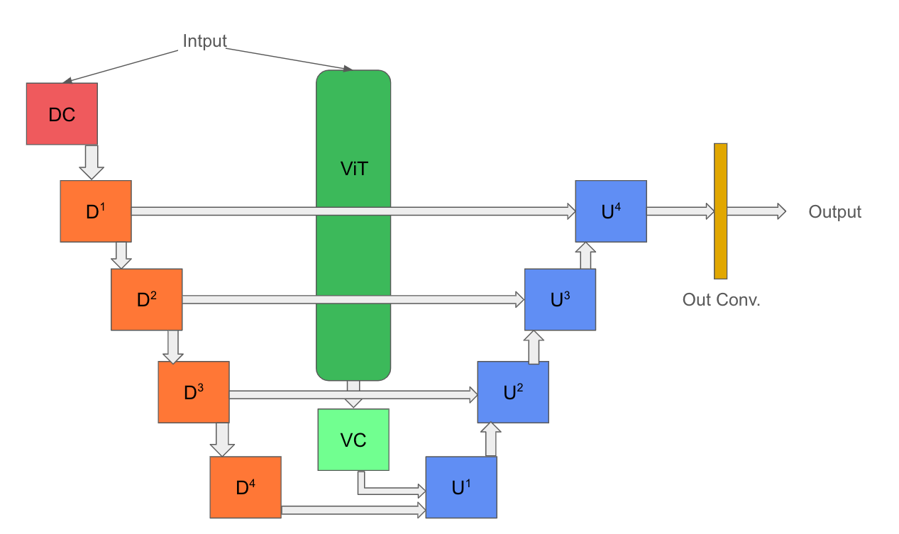
Figure 4: This figure provides a comprehensive view of the ViT-small based U-Net architecture used in our study.In this figure above, DC represents Double Convolution block, $DC^{i}$ represents the $i$th Downsampling block used, $U^{j}$ represents the $j$th upsampling block used. Finally, ViT here represents the Vision-transformer small encoder used and VC represents the Vision Transformer Convolution.

Appendix B Additional Ablation Results

B.1 Change in loss function to cross-entropy

As elucidated in Section 5.2, It is crucial to have a loss function that doesn’t over-fit the majority/dominant class is important. We presented our rationale for using Focal-Tversky loss along with empirical results. Additionally, we also noted cross-entropy tends to overfit the dominant class. In this section we tested this empirically with MedSASS. We trained MedSASS end-to-end on the ISIC-2017 (Codella et al., 2017) dataset for 50 epochs and a batch size of 16. We only swapped the Focal-Tversky loss for a cross-entropy loss while keeping everything else constant. We obtained an IoU on the test set of 0 averaged over five seed values. To investigate further, we observed that the accuracy of the same model averaged over five sedd values was 0.7608±0.002. Representing IoU and accuracy in terms of: TP: True Positive, TN: True Negative, FP: False Positive, and FN: False Negative, we can rewrite IoU and accuracy as:

$IoU=\frac{TP}{TP+FN+FP}$ and $accuracy=\frac{TP+TN}{TP+FN+TN+FP}$.

Since, IoU is 0 hence $TP$ is 0, and since accuracy is non-zero we know that $TP+TN$ has to be non-zero. Given the zero IoU, there are no true positives, meaning the model hasn’t correctly identified and localized any of the objects of interest. Since, $TP$ is 0, $TN$ has to be non-zero. Hence, the architecture has overfit to the background in this case and is predicting background everywhere.

B.2 Change in pre-training epoch and batch size

In Table 5, our investigation focuses on the impact of varying the number of pre-training epochs on the performance of MedSASS, utilizing both ResNet-50 and ViT-small backbones in an end-to-end configuration. Additionally, Tables 7 and 8 are dedicated to exploring how changes in batch size influence MedSASS when trained solely with encoder pre-training. We note that MedSASS demonstrates remarkable resilience against fluctuations in pre-training epochs. For change in the pre-training batch size we observe that although the performance remains constant mostly, there is a slight improvement when we reduce the batch size to 8. This attribute is particularly beneficial for practitioners operating under computational constraints, such as those in developing countries, enabling them to effectively deploy MedSASS. Furthermore, the robust performance of MedSASS with smaller datasets is advantageous for medical image analysis, especially in urgent scenarios like emerging pandemics or diseases lacking established data collection pipelines, such as autoimmune diseases. This capability of MedSASS can significantly contribute to enhancing existing diagnostic and treatment solutions.

Backbone	IoU on Test after pre-training (Epochs)
	10	20	50	70
ResNet50	0.3785 ±0.000249	0.3778 ±0.000568	0.3824 ±0.00579	0.3876 ±0.00098
ViT-small	0.3575 ±0.04	0.3564 ±0.0395	0.3633 ±0.0062	0.4091 ±0.0201

Table 5: In this table, we present IoU averaged over five seed values for encoder-only training on the TissueNet dataset. We observe that the performance of CNNs is almost constant, even with the change in epoch. On the other hand, ViT-small performance increases with an increase in the number of pre-training epochs. This is in line with existing work involving Vision Transformers; this increase in performance is due to the nature of ViTs. While CNN have certain inductive priors, ViTs don’t have them and learn during training.

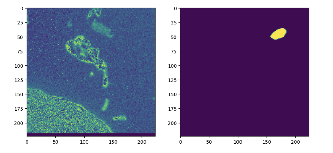
Figure 5: In this figure, we show a sample from the Dermatomyositis dataset, wherein the annotation is incorrect. As we can clearly see, the annotation in mask is at a point where there is blank space (slide background).

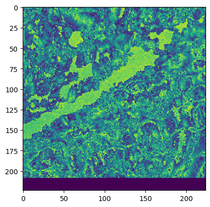
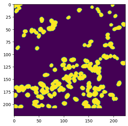
Figure 6: Similar to Figure 5, we have a sample from the Dermatomyositis training set. In many samples within the Dermatomyositis dataset, we observe that the input images are very complex. Additionally, we also observe that, even for the same background, the mask may or may not have cell annotation. This gives an ambiguous supervisory signal and hence the architecture is unable to learn good representations.

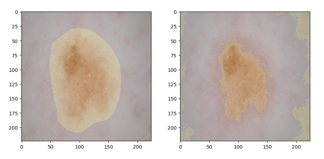
Figure 7: In this figure, we present two images: on the left, the ground truth label superimposed, and on the right, Otsu’s mask superimposed on the input image. In the left pair, i.e the ground truth label and the input image, to train the supervised approach, we observe that, due to the overextending label, the label also covers some light area, This ambiguity makes it hard for the model to learn definitive representations.

Input	Ground Truth	Supervised Prediction	MedSASS Prediction

Table 6: This table showcases three samples randomly chosen from the ISIC-2017 dataset test set, along with their corresponding ground truth masks and the predictions made by both the supervised and MedSASS CNN-based models. In the first row’s sample, it is apparent that the supervised model tends to misclassify even slightly darker regions as the foreground, whereas the MedSASS model slightly underestimates the lesion area. Upon calculating the IoU for these predictions against the ground truth, the supervised model scores 0.3392, while MedSASS achieves a higher score of 0.5473. The second row demonstrates a closer prediction between the two models, with the supervised and MedSASS models attaining IoU scores of 0.6115 and 0.6790, respectively. The third row illustrates the supervised model’s struggle with ambiguous supervision, while MedSASS distinctly segments the lesion with greater clarity. For the final example, Supervised approach records an IoU of 0.4159 as compared to 0.5085 of MedSASS.

Dataset	Batch Size
	8	16	32
ISIC-2017	0.2551 ±0.0243	0.2445 ±0.00482	0.2449 ±0.00968
TissueNet	0.3884 ±0.000241	0.3824 ±0.00579	0.3852 ±0.00607

Table 7: This table presents the Intersection over Union (IoU) averaged across five distinct seed values for the encoder-only training of MedSASS employing a ResNet-50 architecture on the ISIC-2017 and TissueNet datasets, across varying batch sizes. The empirical evidence suggests remarkable stability in performance metrics, notwithstanding alterations in batch size.

Dataset	Batch Size
	8	16	32
ISIC-2017	0.2212 ±0.131	0.1914 ±0.0839	0.2014 ±0.0839
TissueNet	0.413 ±0.033	0.3633 ±0.00624	0.3822 ±0.0204

Table 8: In this table, we present the average IoU over five seed values for encoder-only training of MedSASS with ViT-small backbone on the ISIC-2017 and the TissueNet dataset with different batch sizes. As opposed to CNN, with ViT-small performance improves as we change the batch size, and best performance is observed with a batch size of 8.

Appendix C Comparison with Supervised approach

In addition to comparing MedSASS to other self-supervised approaches for medical image segmentation, we also compared MedSASS with supervised learning. For a fair comparison, we train supervised approaches with focal-tversky loss. Additionally, all approaches were trained for 50 epochs with a batch size of 16. We present these results in Figure 12. All the self-supervised approaches are trained in a label-free manner, i.e., with 0% labels in training, while the supervised approach was trained with 100% labels.

C.1 Curious Case of Dermatomyositis and ISIC-2017 datasets

In Figure 12, we observed that for Dermatomysoitis and the ISIC-2017 dataset, MedSASS outperforms supervised approaches. This happens because some of the labels in the Dermatomysoitis and ISIC-2017 datasets are incorrect. We provide samples of some of these incorrect ground truth labels in Fig. 7 for the ISIC-2017 dataset and in Figures 5 and 6 for the Dermatomyositis dataset. From these figures, we observe that some of the masks for ISIC-2017 overextend the actual lesions. To fix this, we need to perform lession conditioning and sample selection (Ribeiro et al., 2020) to make sure the supervised architecture doesn’t get any ambiguous supervisory signal. Similarly, for the Dermatomyositis dataset, we observe that there are some inconsistencies with the masks as compared to the input. Such inconsistencies for both the ISIC-2017 and the Dermatomyositis result in an ambiguous supervisory signal for supervised learning. Hence, architectures seem to learn a prior where sometimes they classify dark patches as lesions for the ISIC-2017 dataset. We prove this by investigating samples from the test set of our supervised and MedSASS models in Fig 6.

Concerning the Dermatomyositis datasets, we observe that the input images are very complex, and some of the images also have wrong annotations. Due to the complex nature of images, image patches with the same or similar patterns may have different ground truth mask annotations. This ambiguity in the supervisory signal makes it difficult for the architecture to learn meaningful representations. We present these results in Fig. 5 and Fig. 6.

Appendix D Image Classification Performance

As an additional comparison task, we also benchmark MedSASS and other state-of-the-art self-supervised approaches for classification tasks. For this, we use the ISIC-2017 and the X-ray datasets. For this task, we train the encoder for all the techniques, followed by linear probing for multi-class classification. We average the Recall score over the test set for five seed values and present the results in Table 9.

Classification Task Details

• X-Ray dataset Classification task for the X-ray dataset is a multi-class classification task. Each image is classified into one of the four disease categories: normal, lung opacity, COVID, and viral pneumonia. We use the same training, validation, and testing splits as used for segmentation.

• ISIC-2017 dataset Similar to the X-ray dataset task, the classification on the ISIC-2017 dataset is a multi-class classification out of three possible classes: melanoma, nevus-seborrheic keratosis, and healthy. We used the official training, validation, and testing splits of the dataset.

Experimental Details

In this study, we employ self-supervised, pre-trained encoders from both CNN and Transformer architectures, followed by linear probing to assess their representational capabilities. Linear probing is conducted for 50 epochs, incorporating an early stopping criterion with a patience of five epochs to mitigate overfitting. To address the challenge of dataset imbalance, focal loss is strategically utilized. Evaluation is based on the recall score, an effective proxy for the class-balanced F1 score, to ensure equitable performance assessment across classes. For augmentation, use the following sequence: resize to (224,224) $\rightarrow$ (color jitters/random perspective) $\rightarrow$ (color jitter/random affine) $\rightarrow$ random vertical flip $\rightarrow$ random horizontal flip. All experiments were conducted on a single NVIDIA RTX8000 GPU with a batch size of 16.

Arch.	Approach	Recall on ISIC-2017	Recall on X-Ray
ResNet-50	BYOL	0.65 ±0.00815	0.7073±0.0384
	DINO	0.6546±0.00721	0.5241±0.0701
	SimSiam	0.6475 ±0.0104	0.6541 ±0.0466
	MedSASS(e)	0.655 ±0.00845	0.5785±0.0017
ViT-small	MAE	0.6492±0.0101	0.673±0.0173
	SimMIM	0.6438±0.0153	0.66±0.0136
	DINO	0.650±0.0117	0.40±0.0153
	MedSASS(e)	0.6554±0.0087	0.183±0.0255

Table 9: In this table, we present the linear probing results of encoder-only training of MedSASS and other state-of-the-art self-supervised approaches. We observe that for the ISIC-2017 dataset, both CNN and Transformer MedSASS outperform other self-supervised techniques, albeit marginally. On the X-ray dataset, it lags considerably behind in classification performance. The bolded numbers are best reported performance for a particular dataset and architecture, while the underlined are the next best.

Appendix E Drone dataset Performance

The drone dataset (Mostegel et al., 2019) features urban landscapes captured from a nadir perspective, showcasing over 20 residential structures at heights ranging from 5 to 30 meters. High-resolution imagery was obtained using a camera that produces 6000x4000 pixel images. This dataset is richly annotated, containing objects categorized into 23 semantic classes such as unlabeled, paved-area, dirt, grass, gravel, water, rocks, pool, vegetation, roof, wall, window, door, fence, fence-pole, person, dog, car, bicycle, tree, bald-tree, ar-marker, obstacle, and conflicting. We undertake a semantic segmentation task where we differentiate relevant areas—signified by the presence of any objects from the 23 categories—from the background. The outcomes of these experiments are detailed in Sections E.1.

We train encoder-only ResNet-50 methods for 50 epochs with a batch size of 16 and an early-stopping patience of 5 epochs for both binary and multi-class semantic segmentation. We averaged the mean IoU, over three seed values on the test set.

E.1 Semantic segmentation

We present the results of encoder-only training on the drone dataset in Table 10. In this table, we compare the performance of MedSASS and other state-of-the-art self-supervised techniques over three seed values. We used ResNet-50 as our choice of encoder and pre-trained all approaches for 50 epochs.

Approach	Arch.	IoU
SimSiam	ResNet-50	0.9932±0.0345
BYOL	ResNet-50	0.9910±0.0613
MedSASS	ResNet-50	0.9744±0.0445
DINO	ResNet-50	0.9459±0.0527

Table 10: In this table, we present the IoU averaged over three seed values on the test set of the drone dataset. In this task, we performed binary semantic segmentation, wherein we had to segment the objects of interest/foreground (paved area, dirt, grass, gravel, water, rocks, pool, vegetation, roof, wall, window, door, fence, fence-pole, person, dog, car, bicycle, tree, bald-tree, ar-marker, obstacle, and conflicting) from the background. As natural images do not have the same priors as medical images, extracting labels for supervision using Otsu’s approach becomes difficult. Hence, MedSASS is unable to keep up with the state-of-the-art self-supervised technique in this case, but at the same time, it outperformed DINO.

Appendix F On the efficacy of Otsu’s approach

Since MedSASS relies on Otsu’s approach for self-supervision, the quality of output from Otsu’s approach is crucial. In this section, we provide samples of input images, their corresponding ground truths, and their respective output from Otsu’s approach.

F.1 Dermatomyositis Dataset

We present images, the corresponding labels, and the output from Otsu’s approach for samples from the Dermatomyositis dataset in Figure 8. We observe that while the output from Otsu’s approach is not identical to the ground truth images, they are similar enough to be used for supervision instead of the actual ground truth images. Additionally, the Dermatomyositis dataset is a challenging dataset due to the complexity and large number of small objects present in the dataset (as presented in Fig. 8), along with the limited number of samples available in the dataset.

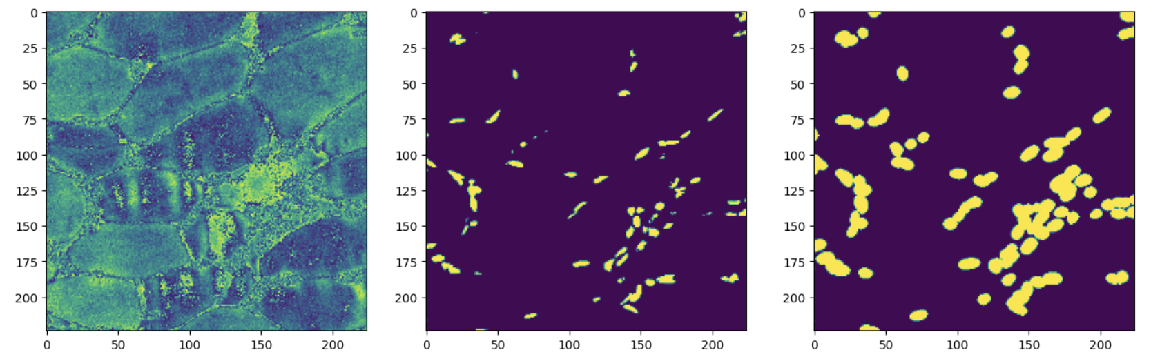
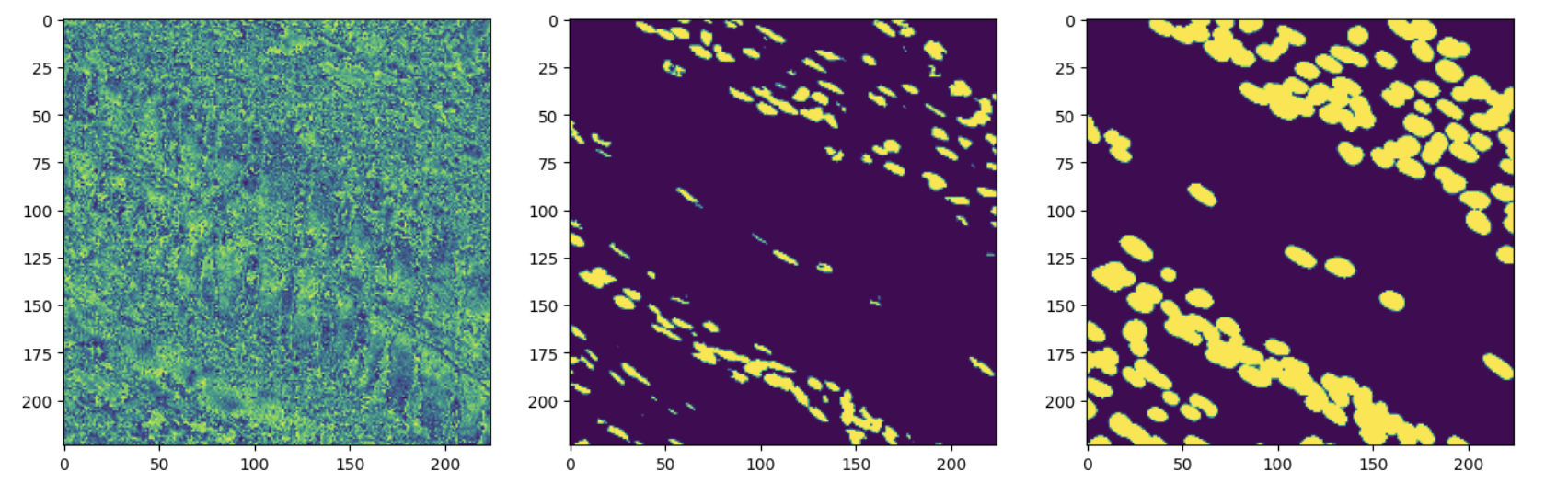
Figure 8: In this figure, we show two samples from the Dermatomyositis dataset (Singh & Cirrone, 2023; Van Buren et al., 2022). In the rightmost column, we have the input image; in center column, we present the output from Otsu’s approach, and finally, the corresponding ground truth image is in the rightmost column.

F.2 ISIC-2017 Dataset

Similarly, we present samples from the ISIC-2017 dataset in Figure 9. Additionally, in Section C.1, we observed that some of the labels might require label conditioning (Ribeiro et al., 2020), and Otsu’s output can provide better labels for learning; hence, MedSASS with Otsu label supervision outperforms the supervised approach on the ISIC-2017 dataset. The ISIC-2017 dataset is a particularly challenging dataset due to small inter-class variation and obfuscation of the lesion region (Singh & Cirrone, 2023).

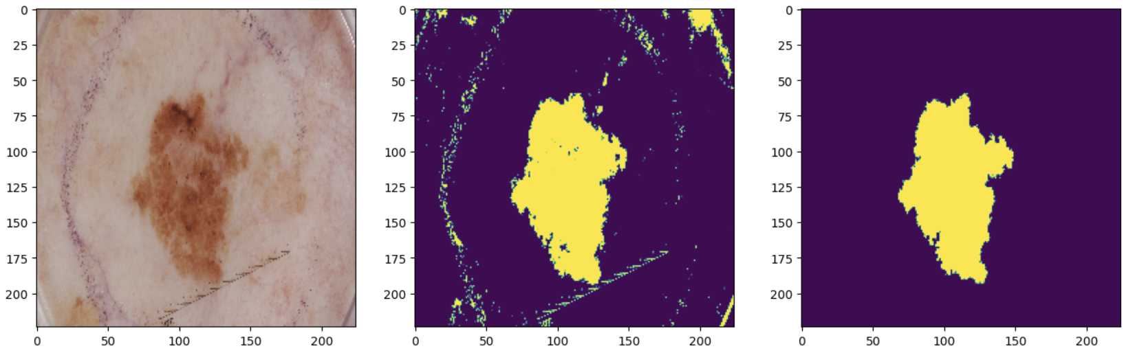
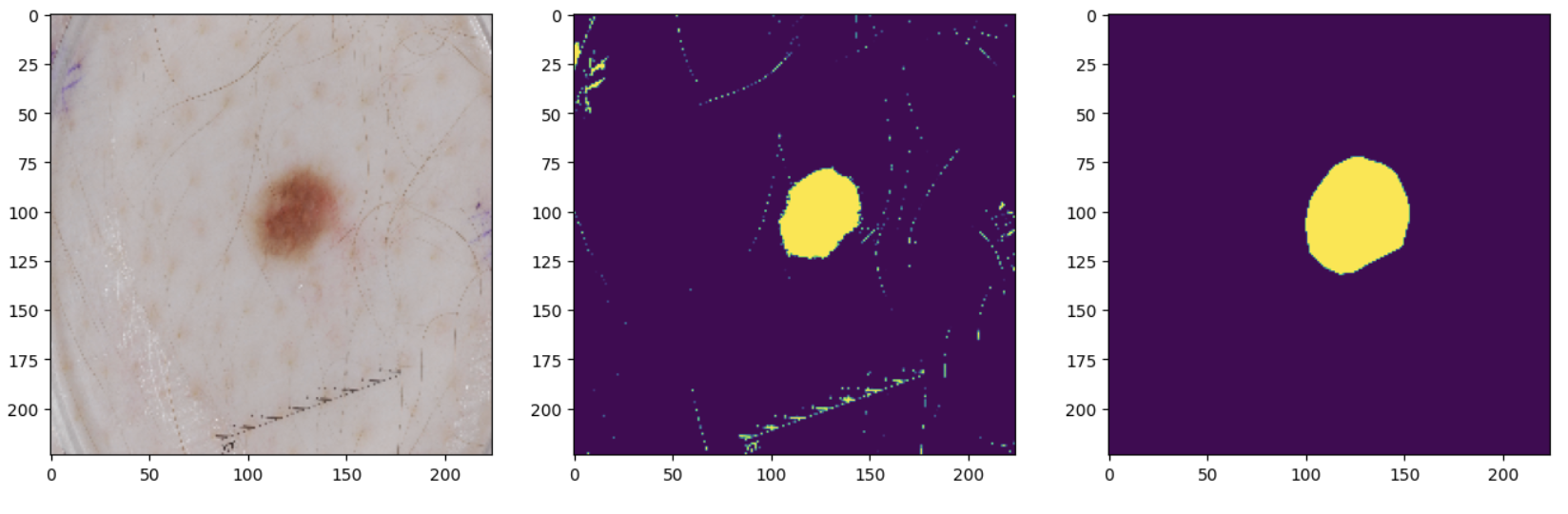
Figure 9: In this figure, we show two samples from the ISIC-2017 (Codella et al., 2017) dataset. In the rightmost column, we have the input image; in center column, we present the output from Otsu’s approach, and finally, the corresponding ground truth image is in the rightmost column.

F.3 Tissuenet Dataset

In Fig. 10, we present the input image in the leftmost column, Otsu’s output in the middle, and the corresponding ground truth for the input image in the rightmost column. Similar to the Dermatomyositis dataset, this dataset also contains a large number of small objects. The TissueNet dataset came from a number of different imaging platforms, such as CODEX, Cyclic Immunofluorescence, IMC, MIBI, Vectra, and MxIF. It shows a wide range of disease states and tissue types. Furthermore, this dataset consists of paired nuclear and whole-cell annotations, which, when combined, sum up to more than one million paired annotations. (Greenwald et al., 2022).

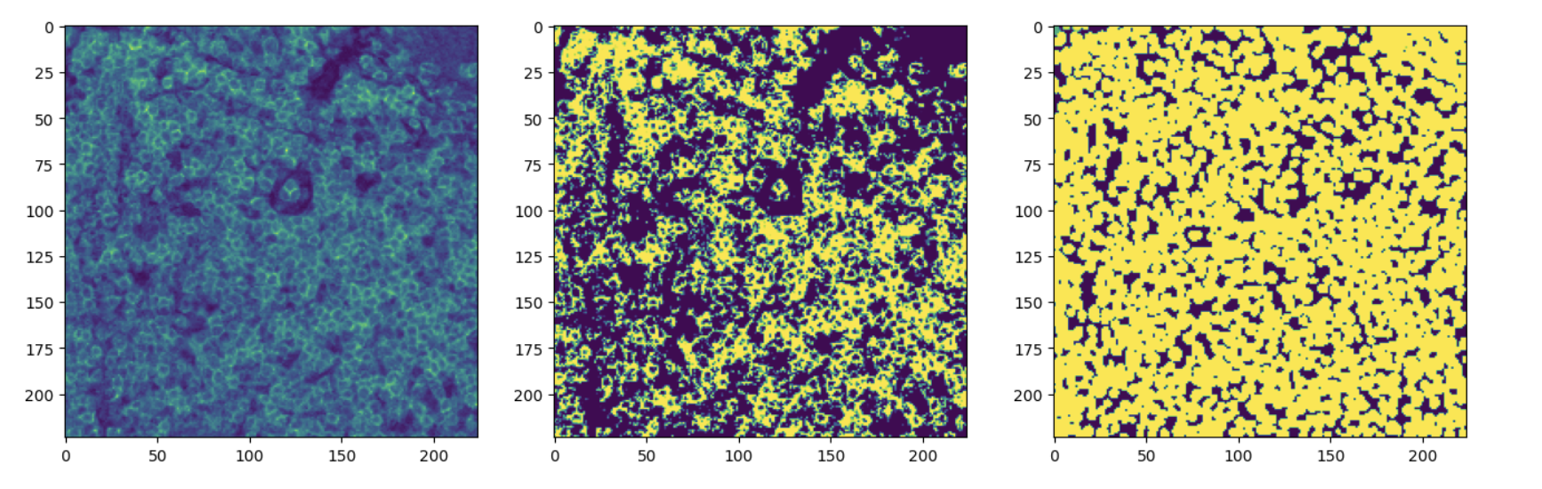
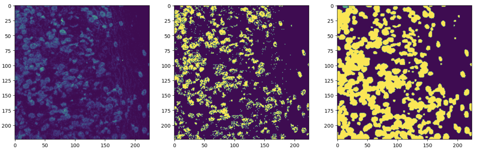
Figure 10: Sample images from the TissueNet dataset (Greenwald et al., 2022), similar to Fig. 8 and 9, in the leftmost column we have the input images, output from Otsu in middle and ground truth corresponding to the input image in the rightmost column.

F.4 X-Ray Dataset

X-ray imaging stands as a predominant diagnostic tool due to its widespread availability, cost-effectiveness, non-invasiveness, and simplicity. But lung segmentation is hard because of three things: (1) changes that are not the result of disease, such as changes in lung shape and size due to age, gender, and heart size; (2) changes that are the result of disease, such as high-intensity opacities brought on by severe pulmonary conditions; and (3) obfuscation in imaging, such as clothing or medical devices (pacemakers, infusion tubes, catheters) that cover the lung field. We present two samples from the X-ray dataset in Fig. 11 along with their Otsu’s output and corresponding ground truth. Despite the challenges for each dataset we observe that Otsu’s labels provide non-blank and masks that are similar to the ground truth.

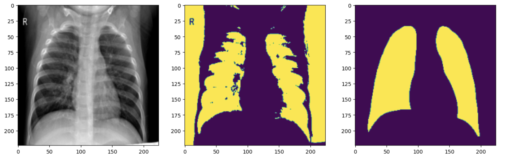
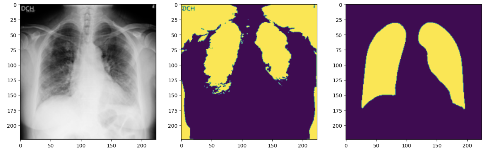
Figure 11: Sample images from the X-ray dataset (Chowdhury et al., 2020; Rahman et al., 2021) are displayed as follows: the leftmost column features the input images, the center column presents the output from Otsu, and the rightmost column showcases the ground truth corresponding to each input image.

(a)

(b)

Figure 12: This figure provides a comparative analysis of different training methodologies: traditional supervised training, MedSASS with both encoder and decoder (MedSASS (E+D)), MedSASS with only the encoder (MedSASS (E)), and other leading self-supervised techniques. The black dot atop each bar, connected by a horizontal line, signifies the error bar derived from averaging over five different seed values. Notably, MedSASS (E+D) surpasses supervised training for CNNs on the Dermatomyositis and ISIC-2017 datasets and achieves equivalent results for ViTs. We present the result for CNN and ViT-small backbones in part (a) and (b) respectively of the figure. We discuss this phenomenon in greater detail in Section C.1. Furthermore, we note a significant performance disparity between supervised training and current state-of-the-art self-supervised techniques, with MedSASS generally bridging this performance gap.

Appendix G Description of Metrics

For segmentation

For measuring segmentation performance, we use the IoU, or Intersection Over Union, metric. It helps us understand how similar the sample sets are.

$IoU=\frac{\text{area of overlap}}{\text{area of union}}=\frac{\leavevmode\hbox to72.33pt{\vbox to72.33pt{\text{[drawing]}}}}{\leavevmode\hbox to72.33pt{\vbox to72.33pt{\text{[drawing]}}}}$

For classification

we used the recall score as our comparison metric for multi-class classification, which is defined as $Recall=\frac{TP}{TP+FN}$, where TP: True Positive, TN: True Negative, FP: False Positive, and FN: False Negative. Since, both the datasets have class imbalance to get a real sense of performance we use Recall value. This is because it is semantically equal to the balanced multi-class accuracy value, TP: True Positive, TN: True Negative, FP: False Positive, and FN: False Negative.

References

- Abraham & Khan (2019) Abraham, N. and Khan, N. M. A novel focal tversky loss function with improved attention u-net for lesion segmentation. In 2019 IEEE 16th international symposium on biomedical imaging (ISBI 2019), pp. 683–687. IEEE, 2019.
- Barron (2020) Barron, J. T. A generalization of otsu’s method and minimum error thresholding. In Computer Vision–ECCV 2020: 16th European Conference, Glasgow, UK, August 23–28, 2020, Proceedings, Part V 16, pp. 455–470. Springer, 2020.
- Caron et al. (2020) Caron, M., Misra, I., Mairal, J., Goyal, P., Bojanowski, P., and Joulin, A. Unsupervised learning of visual features by contrasting cluster assignments. Advances in Neural Information Processing Systems, 33:9912–9924, 2020.
- Caron et al. (2021) Caron, M., Touvron, H., Misra, I., Jégou, H., Mairal, J., Bojanowski, P., and Joulin, A. Emerging properties in self-supervised vision transformers. In Proceedings of the IEEE/CVF international conference on computer vision, pp. 9650–9660, 2021.
- Chan et al. (1998) Chan, F., Lam, F., and Zhu, H. Adaptive thresholding by variational method. IEEE Transactions on Image Processing, 7(3):468–473, 1998. doi: 10.1109/83.661196.
- Chen et al. (2020) Chen, T., Kornblith, S., Norouzi, M., and Hinton, G. E. A simple framework for contrastive learning of visual representations. ArXiv, abs/2002.05709, 2020.
- Chen & He (2021) Chen, X. and He, K. Exploring simple siamese representation learning. 2021 IEEE/CVF Conference on Computer Vision and Pattern Recognition (CVPR), pp. 15745–15753, 2021.
- Chowdhury et al. (2020) Chowdhury, M. E., Rahman, T., Khandakar, A., Mazhar, R., Kadir, M. A., Mahbub, Z. B., Islam, K. R., Khan, M. S., Iqbal, A., Al Emadi, N., et al. Can ai help in screening viral and covid-19 pneumonia? Ieee Access, 8:132665–132676, 2020.
- Codella et al. (2017) Codella, N., Gutman, D., Celebi, M., Helba, B., Marchetti, M., Dusza, S., Kalloo, A., Liopyris, K., Mishra, N., and Kittler, H. Skin lesion analysis toward melanoma detection: A challenge at the 2017 international symposium on biomedical imaging. Int Skin Imag Collab (ISIC). arXiv Prepr arXiv171005006, 2017.
- Dance et al. (2014) Dance, D., Christofides, S., Maidment, A., McLean, I., and Ng, K. Diagnostic radiology physics. International Atomic Energy Agency, 299, 2014.
- Godard et al. (2019) Godard, C., Mac Aodha, O., Firman, M., and Brostow, G. J. Digging into self-supervised monocular depth estimation. In Proceedings of the IEEE/CVF international conference on computer vision, pp. 3828–3838, 2019.
- Greenwald et al. (2022) Greenwald, N. F., Miller, G., Moen, E., Kong, A., Kagel, A., Dougherty, T., Fullaway, C. C., McIntosh, B. J., Leow, K. X., Schwartz, M. S., et al. Whole-cell segmentation of tissue images with human-level performance using large-scale data annotation and deep learning. Nature biotechnology, 40(4):555–565, 2022.
- Grill et al. (2020) Grill, J.-B., Strub, F., Altché, F., Tallec, C., Richemond, P., Buchatskaya, E., Doersch, C., Avila Pires, B., Guo, Z., Gheshlaghi Azar, M., et al. Bootstrap your own latent-a new approach to self-supervised learning. Advances in neural information processing systems, 33:21271–21284, 2020.
- He et al. (2015) He, K., Zhang, X., Ren, S., and Sun, J. Deep residual learning for image recognition. corr abs/1512.03385 (2015), 2015.
- He et al. (2020) He, K., Fan, H., Wu, Y., Xie, S., and Girshick, R. B. Momentum contrast for unsupervised visual representation learning. 2020 IEEE/CVF Conference on Computer Vision and Pattern Recognition (CVPR), pp. 9726–9735, 2020.
- He et al. (2022) He, K., Chen, X., Xie, S., Li, Y., Dollár, P., and Girshick, R. Masked autoencoders are scalable vision learners. In Proceedings of the IEEE/CVF Conference on Computer Vision and Pattern Recognition, pp. 16000–16009, 2022.
- Iakubovskii (2019) Iakubovskii, P. Segmentation models pytorch. https://github.com/qubvel/segmentation_models.pytorch, 2019.
- Jabri et al. (2020) Jabri, A., Owens, A., and Efros, A. Space-time correspondence as a contrastive random walk. Advances in neural information processing systems, 33:19545–19560, 2020.
- Kalapos & Gyires-Tóth (2022) Kalapos, A. and Gyires-Tóth, B. Self-supervised pretraining for 2d medical image segmentation. In European Conference on Computer Vision, pp. 472–484. Springer, 2022.
- Kittler & Illingworth (1986) Kittler, J. and Illingworth, J. Minimum error thresholding. Pattern recognition, 19(1):41–47, 1986.
- Kleinberg et al. (2022) Kleinberg, G., Diaz, M. J., Batchu, S., and Lucke-Wold, B. Racial underrepresentation in dermatological datasets leads to biased machine learning models and inequitable healthcare. Journal of biomed research, 3(1):42, 2022.
- Kumar et al. (2017) Kumar, N., Verma, R., Sharma, S., Bhargava, S., Vahadane, A., and Sethi, A. A dataset and a technique for generalized nuclear segmentation for computational pathology. IEEE transactions on medical imaging, 36(7):1550–1560, 2017.
- Lin et al. (2017) Lin, T.-Y., Goyal, P., Girshick, R., He, K., and Dollár, P. Focal loss for dense object detection. In Proceedings of the IEEE international conference on computer vision, pp. 2980–2988, 2017.
- Litjens et al. (2017) Litjens, G., Kooi, T., Bejnordi, B. E., Setio, A. A. A., Ciompi, F., Ghafoorian, M., Van Der Laak, J. A., Van Ginneken, B., and Sánchez, C. I. A survey on deep learning in medical image analysis. Medical image analysis, 42:60–88, 2017.
- Mostegel et al. (2019) Mostegel, C., Maurer, M., Heran, N., Puerta, J., and Fraundorfer, F. Semantic drone dataset. http://dronedataset.icg.tugraz.at, 2019.
- Otsu (1979) Otsu, N. A threshold selection method from gray-level histograms. IEEE transactions on systems, man, and cybernetics, 9(1):62–66, 1979.
- Paszke et al. (2019) Paszke, A., Gross, S., Massa, F., Lerer, A., Bradbury, J., Chanan, G., Killeen, T., Lin, Z., Gimelshein, N., Antiga, L., et al. Pytorch: An imperative style, high-performance deep learning library. Advances in neural information processing systems, 32, 2019.
- Pham et al. (2000) Pham, D. L., Xu, C., and Prince, J. L. Current methods in medical image segmentation. Annual review of biomedical engineering, 2(1):315–337, 2000.
- Rahman et al. (2021) Rahman, T., Khandakar, A., Qiblawey, Y., Tahir, A., Kiranyaz, S., Kashem, S. B. A., Islam, M. T., Al Maadeed, S., Zughaier, S. M., Khan, M. S., et al. Exploring the effect of image enhancement techniques on covid-19 detection using chest x-ray images. Computers in biology and medicine, 132:104319, 2021.
- Ribeiro et al. (2020) Ribeiro, V., Avila, S., and Valle, E. Less is more: Sample selection and label conditioning improve skin lesion segmentation. In Proceedings of the IEEE/CVF Conference on Computer Vision and Pattern Recognition Workshops, pp. 738–739, 2020.
- Ronneberger et al. (2015) Ronneberger, O., Fischer, P., and Brox, T. U-net: Convolutional networks for biomedical image segmentation. In International Conference on Medical image computing and computer-assisted intervention, pp. 234–241. Springer, 2015.
- Salehi et al. (2017) Salehi, S. S. M., Erdogmus, D., and Gholipour, A. Tversky loss function for image segmentation using 3d fully convolutional deep networks. In International workshop on machine learning in medical imaging, pp. 379–387. Springer, 2017.
- Singh & Cirrone (2023) Singh, P. and Cirrone, J. A data-efficient deep learning framework for segmentation and classification of histopathology images. In Computer Vision–ECCV 2022 Workshops: Tel Aviv, Israel, October 23–27, 2022, Proceedings, Part III, pp. 385–405. Springer, 2023.
- Singh et al. (2023) Singh, P., Chen, L., Chen, M., Pan, J., Chukkapalli, R., Chaudhari, S., and Cirrone, J. Enhancing medical image segmentation: Optimizing cross-entropy weights and post-processing with autoencoders. In Proceedings of the IEEE/CVF International Conference on Computer Vision (ICCV) Workshops, pp. 2684–2693, October 2023.
- Sudre et al. (2017) Sudre, C. H., Li, W., Vercauteren, T., Ourselin, S., and Jorge Cardoso, M. Generalised dice overlap as a deep learning loss function for highly unbalanced segmentations. In Deep Learning in Medical Image Analysis and Multimodal Learning for Clinical Decision Support: Third International Workshop, DLMIA 2017, and 7th International Workshop, ML-CDS 2017, Held in Conjunction with MICCAI 2017, Québec City, QC, Canada, September 14, Proceedings 3, pp. 240–248. Springer, 2017.
- Van Buren et al. (2022) Van Buren, K., Li, Y., Zhong, F., Ding, Y., Puranik, A., Loomis, C. A., Razavian, N., and Niewold, T. B. Artificial intelligence and deep learning to map immune cell types in inflamed human tissue. Journal of Immunological Methods, 505:113233, 2022. ISSN 0022-1759. doi: https://doi.org/10.1016/j.jim.2022.113233. URL https://www.sciencedirect.com/science/article/pii/S0022175922000205.
- Xie et al. (2022) Xie, Z., Zhang, Z., Cao, Y., Lin, Y., Bao, J., Yao, Z., Dai, Q., and Hu, H. Simmim: A simple framework for masked image modeling. In Proceedings of the IEEE/CVF Conference on Computer Vision and Pattern Recognition, pp. 9653–9663, 2022.