Nonlinear subspace clustering by functional link neural networks

Abstract

Nonlinear subspace clustering based on a feed-forward neural network has been demonstrated to provide better clustering accuracy than some advanced subspace clustering algorithms. While this approach demonstrates impressive outcomes, it involves a balance between effectiveness and computational cost. In this study, we employ a functional link neural network to transform data samples into a nonlinear domain. Subsequently, we acquire a self-representation matrix through a learning mechanism that builds upon the mapped samples. As the functional link neural network is a single-layer neural network, our proposed method achieves high computational efficiency while ensuring desirable clustering performance. By incorporating the local similarity regularization to enhance the grouping effect, our proposed method further improves the quality of the clustering results. Additionally, we introduce a convex combination subspace clustering scheme, which combining a linear subspace clustering method with the functional link neural network subspace clustering approach. This combination approach allows for a dynamic balance between linear and nonlinear representations. Extensive experiments confirm the advancement of our methods. The source code will be released on https://lshi91.github.io/ soon.

1 Introduction

Subspace clustering involves the objective of identifying clusters within data points distributed across distinct subspaces in a high-dimensional space [1, 2]. Its practical applications encompass various scenarios, including image segmentation [3, 4], motion segmentation [5, 6], face grouping [7, 8], character identification [9, 10], among others. The categorization of subspace clustering methods generally comprises four classes: algebraic approaches [11], iterative techniques [12], statistical methodologies [13, 14], and methods based on spectral clustering [15, 16]. Notably, spectral clustering-based techniques have garnered considerable attention due to their superior clustering performance. In essence, spectral clustering-based methods entail fundamental stages: 1) initial acquisition of a representation matrix to establish a similarity matrix derived from original data points, 2) subsequent execution of spectral decomposition and $k$-means clustering to derive the ultimate cluster assignments.

Over the last decade, several subspace clustering techniques have emerged in literature, all aiming to uncover the underlying data subspace structure. The most popular spectral clustering algorithms are Sparse Subspace Clustering (SSC) [3] and Low Rank Representation (LRR) [5]. These methods enable sparse or minimum rank representation of data samples, respectively. Specifically, SSC operates under the assumption that each subspace can be expressed as a sparse linear combination of other points, while LRR aims to create a low-rank matrix that captures the overall data structure. To preserve both the global and local data structures, some researchers have explored incorporating constraints related to low rank and sparsity [17, 18, 19]. The Frobenius norm is applied to the representation matrix in the Least Squares Regression (LSR) algorithm [20], with the goal of establishing the block diagonal characteristic within both inter-cluster and intra-cluster affinities. [21] merges SSC and LSR through the utilization of the trace Lasso technique. This adaptive approach enables the dynamic selection and clustering of correlated data. Lu et al. put forth an innovative regularization strategy relying on the block diagonal matrix, directly imposing the block diagonal structure onto the Block Diagonal Representation (BDR) [9]. Hu et al presented the grouping effect as the extent to which a representation matrix reflects the cluster structure of data points and developed the Smooth Representation Clustering (SMR) model [22], which incorporates a smoothness regularizer to impose the grouping effect and a least squares error term to fit the data. Moreover, the author also introduced a novel affinity measure that leverages the grouping effect, which shows better performance than the conventional one. To deal with complex noise that often occurs in real-world scenarios, some robust subspace clustering algorithms based on maximum correntropy criterion [23, 24] have been reported [25, 26, 27].

Many existing techniques for subspace clustering rely on leveraging the linear connections between samples to learn the affinity matrix. In deed, in many practical scenarios, data samples often exhibit nonlinear relationships. The previous mentioned subspace clustering methods may experience performance degradation when dealing with such nonlinear data samples, thereby motivating the development of nonlinear subspace clustering methods. As a typical category of non-linear techniques, kernel-based subspace clustering methods have gained popularity. These methods possess the capability to perform a nonlinear transformation [28, 29, 30, 31, 32]. One such example is the Kernel Sparse Subspace Clustering (KSSC) [28], which incorporates the kernel method into SSC, enabling the algorithm to find a nonlinear decision boundary that can separate the data more effectively. Kang et al introduced a comprehensive framework that unifies graph construction and kernel learning, harnessing the resemblance of the kernel matrix to enhance clustering performance [33]. Zhen et al enhanced the algorithm robustness and guaranteed the block diagonal property by truncating the trivial coefficients of kernel matrix [31]. Multi-kernel learning methods have been used to find the optimal kernel combination for better clustering results [34, 35]. In addition to the kernel method, Zhu et al employed a feed-forward neural network for executing nonlinear mapping and subsequently introduced the Nonlinear Subspace Clustering (NSC) technique [36]. Deep Subspace Clustering (DSC) techniques that combine the advantages of deep neural networks and subspace clustering methods have drawn much attention [37], which introduce a self-expression layer between the encoder and the decoder to learn a similarity graph. However, subspace clustering methods based on neural network have limitations in computational cost when the layer number is large, and may also be sensitive to the setting of hyperparameters [38].

To address the aforementioned challenge, this paper introduces an innovative subspace clustering technique that utilizes the functional link neural network (FLNN). This approach is termed Functional Link Neural Network Subspace Clustering (FLNNSC). FLNN is a single-layer artificial neural network that applies nonlinear transformations to the input features to strengthen the learning capability of the network [39, 40, 41]. Compared with the conventional neural network, FLNN is able to achieve comparable function approximation performance with faster convergence and lower computational complexity. In practical scenarios, data often exhibit both linear and nonlinear structures. To fully exploit both the linear and nonlinear features of the data, we propose an extension of FLNNSC, introducing a convex combination subspace clustering (CCSC) method that simultaneously integrates linear and nonlinear representations. Our main contributions are summarized as follows:

1. We investigate a novel method known as FLNNSC for nonlinear subspace clustering. This method is highly effective in exploiting the nonlinear relations of data points. It also effectively captures local similarity through the grouping effect and mitigates overfitting by imposing a weight regularization mechanism. To solve the optimization problem for FLNNSC, we develop an iterative optimization algorithm.

2. By integrating linear and nonlinear representations, we propose a CCSC method, allowing for a comprehensive exploration and exploitation of the data’s diverse features.

3. By conducting experiments on widely recognized datasets, we confirm the superiority of our advanced subspace clustering approaches.

The organization of the paper is as follows. Section 2 offers a review of relevant subspace clustering methods. In Section 3, we introduce our novel subspace clustering approach. The evaluation of our methods’ performance across diverse datasets is conducted in Section 4. Conclusions are drawn in Section 5.

Notations. The main notations used in the paper are summarized in Table 1.

Table 1: Notations used in this paper.

Notation	Description
$\mathbf{X}$	data matrix
$\mathbf{Z}$	self-representation matrix
$\lVert\cdot\rVert_{1}$	$l_{1}$-norm of a matrix
$diag(\cdot)$	diagonal entries of a matrix
$\lVert\cdot\rVert_{2,1}$	$l_{2,1}$-norm of a matrix
$\lVert\cdot\rVert_{*}$	nuclear norm
$\lVert\cdot\rVert_{F}$	$F$-norm of a matrix
${\rm Tr}(\cdot)$	trace of a matrix
$\odot$	element-wise product
$(\cdot)^{T}$	tranpose of a vector or a matrix

2 Related work

In this section, we briefly review SSC [3] and LRR [5]. To facilitate our review, we first present some relevant definitions and notations. Let $\mathbf{X}=[\mathbf{x}_{1},\mathbf{x}_{2},\cdots,\mathbf{x}_{n}]\in\mathbb{R}^{d\times n}$ and $\mathbf{Z}=[\mathbf{z}_{1},\mathbf{z}_{2},\cdots,\mathbf{z}_{n}]\in\mathbb{R}^{n\times n}$ denote the data matrix and self-representation matrix, respectively, where $\mathbf{x}_{i}$ is the $i$th sample of $\mathbf{X}$, $d$ denotes the data dimension, and $n$ is the data number.

The objective of SSC is to uncover the sparse linear structure of data points. This is achieved by imposing the constraint of sparsity upon the representation matrix, which can be expressed as follows:

$$\mathop{\rm min}\limits_{\mathbf{Z}}\\ \ \lVert\mathbf{Z}\rVert_{1},\quad s.t.\mathbf{X}=\mathbf{X}\mathbf{Z},diag(\mathbf{Z})=0$$ (1)

where the utilization of the $l_{1}$-norm serves the purpose of pursuing a sparse representation, the vector $diag(\cdot)\in\mathbb{R}^{n}$ is constructed from the diagonal entries of $\mathbf{Z}$, and the constraint $diag(\mathbf{Z})=\mathbf{0}$ is imposed to prevent the emergence of trivial solutions. Solving the optimization problem as stated in (1) can be achieved by implementing the Alternating Direction Method of Multipliers (ADMM) [42].

LRR utilizes the inherent property of low rank to capture the global features of data. The formulation of the corresponding objective function is presented as:

$$\mathop{\rm min}\limits_{\mathbf{Z}}\\ \ \lVert\mathbf{X}-\mathbf{X}\mathbf{Z}\rVert_{2,1}+\lambda\lVert\mathbf{Z}\rVert_{*}$$ (2)

where the $l_{2,1}$-norm is employed to enforce row sparsity on the error matrix, enabling the identification and removal of outliers that diverge from the underlying subspaces, $\lVert\mathbf{Z}\rVert_{*}$ computes the summation of singular values within $\mathbf{Z}$, and $\lambda$ is a balance parameter. A notable distinction between SSC and LRR lies in their methodologies: SSC relies on the $l_{1}$-norm to induce sparsity, whereas LRR utilizes the nuclear norm to encourage a low-rank structure.

3 FLNN subspace clustering

This section first presents the basic principle of functional link neural network. Subsequently, we present the formulation of our novel model along with the procedures for optimization. The framework of our proposed FLNNSC method is shown in Figure 1.

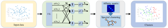
Figure 1: Framework of FLNNSC, where $\mathbf{F.E.}$ in a FLNN represents the functional expansion module.

3.1 Functional link neural network

It is seen from the second panel of Figure 1 that the FLNN is a single-layer neural network, comprised of an input layer that is functionally expanded and an accompanying output layer. Notably, there is an absence of a hidden layer within this configuration. The input layer can be expanded by some nonlinear functions such as Chebyshev polynomials, Legendre polynomials, trigonometric functions, etc, which is useful to strengthen the learning capability of the network. For example, consider the $i$th element $x_{i}$ in a vector $\mathbf{x}$, an enhanced representation by using a second-order trigonometric polynomial is given by $\varphi(x_{i})=[x_{i},\sin(\pi x_{i}),\cos(\pi x_{i}),\sin(2\pi x_{i}),\cos(2\pi x_{i})]$. The FLNN has a simpler structure than the traditional feed-forward neural network, as it does not have any hidden layers. This reduces the computational complexity and the number of parameters that need to be trained.

3.2 Model formulation

As described above, we denote $\mathbf{X}=[\mathbf{x}_{1},\mathbf{x}_{2},\cdots,\mathbf{x}_{n}]\in\mathbb{R}^{d\times n}$ and $\mathbf{Z}=[\mathbf{z}_{1},\mathbf{z}_{2},\cdots,\mathbf{z}_{n}]\in\mathbb{R}^{n\times n}$ as the data matrix and self-representation matrix, respectively. The input sample $\mathbf{x}_{i}$ is expanded by a nonlinear function $\varphi(\cdot)$, and then pass through a layer of multiple neurons. With an activation function, the output is provided by

$$\mathbf{h}_{i}=\rho(\mathbf{W}\varphi(\mathbf{x}_{i})),\qquad i=1,\cdots,n$$ (3)

where $\mathbf{h}_{i}\in\mathbb{R}^{\hat{d}\times 1}$ represents the output vector with $\hat{d}$ being the expanded dimension via functional expansion, $\rho(\cdot)$ denotes the activation function, $\mathbf{W}\in\mathbb{R}^{\hat{d}\times\hat{d}}$ is the parameter matrix to be trained, which plays a pivotal role in generating outputs that closely approximate the actual results, and $\varphi(\mathbf{x}_{i})\in\mathbb{R}^{\hat{d}\times 1}$ is the input vector after functional expansion. In this paper, we select a typical expansion function, namely trigonometric polynomial, for $\varphi(\mathbf{x}_{i})$. The choice of trigonometric polynomials is motivated by their inherent simplicity and computational efficiency. Moreover, they provide orthonormal bases, a feature that greatly simplifies the process of calculating expansion coefficients, thereby enhancing the overall computational performance. Specifically, we employ a second-order expansion because it achieves a balance between performance and computational complexity. While higher-order expansions could potentially be used, they would significantly increase the computational complexity. We find that a second-order expansion is sufficient to achieve good performance while maintaining an acceptable level of complexity. Consequently, the dimension of the transformed data is $\hat{d}=5d$.

By stacking each $\mathbf{h}_{i}$, the output matrix $\mathbf{H}$ of the output layer is defined as

$$\mathbf{H}=[\mathbf{h}_{1},\mathbf{h}_{2},\cdots,\mathbf{h}_{n}]$$ (4)

Using the output matrix $\mathbf{H}$, our approach conducts subspace clustering in the nonlinear domain.

The objective function $J$ of FLNNSC is comprised of three components, i.e.,

$$\mathop{\rm min}\limits_{\mathbf{W},\mathbf{Z}}J=J_{1}+J_{2}+J_{3},$$ (5)

where $J_{1}$ is served to learn the self-representation matrix, $J_{2}$ is used to impose the grouping effect, and $J_{3}$ is employed to avoid the model over-fitting.

Specifically, we define $J_{1}$ as

$$J_{1}=\frac{1}{2}\sum^{n}_{i=1}\lVert\mathbf{h}_{i}-\mathbf{H}\mathbf{z}_{i}\rVert^{2}_{F}.$$ (6)

The second component $J_{2}$ is defined as

$$J_{2}=\frac{\alpha}{2}{\rm Tr}(\mathbf{Z}\mathbf{L}\mathbf{Z}^{T}),$$ (7)

where $\alpha$ is a balance parameter, the Laplacian matrix $\mathbf{L}$ is determined through the calculation $\mathbf{L}=\mathbf{D}-\mathbf{S}$ with $\mathbf{S}$ measuring the data similarity, and $\mathbf{D}$ being a diagonal matrix with its diagonal entries calculated by $D_{ii}=\sum^{n}_{j=1}S_{ij}$. A prevalent approach to construct $\mathbf{S}$ involves the use of a $k$ nearest neighbor ($k$-nn) graph, coupled with either a heat kernel or $0$-$1$ weights [22]. The third component $J_{3}$ is defined as

$$J_{3}=\frac{\beta}{2}\lVert\mathbf{W}\rVert^{2}_{F},$$ (8)

where $\beta$ is a regularization parameter.

Combining (6), (7) and (8), FLNNSC can be explicitly defined as

$$J=\mathop{\rm min}\limits_{\mathbf{W},\mathbf{Z}}\left\{\frac{1}{2}\sum^{n}_{i=1}\lVert\mathbf{h}_{i}-\mathbf{H}\mathbf{z}_{i}\rVert^{2}_{F}+\frac{\alpha}{2}{\rm Tr}(\mathbf{Z}\mathbf{L}\mathbf{Z}^{T})+\frac{\beta}{2}\lVert\mathbf{W}\rVert^{2}_{F}\right\}$$ (9)

The formulated model is capable of exploiting the nonlinearity of data and manipulating the local structure features.

3.3 Optimization

In this section, we comprehensively detail the process of addressing the optimization problem specified in equation (9). Note that the optimization problem depends on two variables, $\mathbf{W}$ and $\mathbf{Z}$. In the subsequent derivation, we update $\mathbf{W}$ and $\mathbf{Z}$ iteratively.

1) Update $\mathbf{W}$: To update $\mathbf{W}$, we keep $\mathbf{H}$ and $\mathbf{Z}$ fixed and eliminate the irrelevant term, and arrive at

$$\mathop{\rm min}\limits_{\mathbf{W}}\left\{\frac{1}{2}\sum^{n}_{i=1}\lVert\mathbf{h}_{i}-\mathbf{H}\mathbf{z}_{i}\rVert^{2}_{F}+\frac{\beta}{2}\lVert\mathbf{W}\rVert^{2}_{F}\right\}.$$ (10)

A direct method to tackle the optimization problem stated in (10) is by employing the gradient descent algorithm. Upon calculating the derivative of the aforementioned objective function with respect to $\mathbf{W}$, we obtain

$$\frac{\partial J}{\partial\mathbf{W}}=(\mathbf{h}_{i}-\mathbf{H}\mathbf{z}_{i})\odot\rho^{\prime}(\mathbf{W}\varphi(\mathbf{x}_{i}))\varphi^{T}(\mathbf{x}_{i})+\beta\mathbf{W},$$ (11)

where $\rho^{\prime}(\cdot)$ represents the derivative of the activation function $\rho(\cdot)$. As a result, the parameter matrix $\mathbf{W}$ is updated as

$$\mathbf{W}=\mathbf{W}-\mu\left[(\mathbf{h}_{i}-\mathbf{H}\mathbf{z}_{i})\odot\rho^{\prime}(\mathbf{W}\varphi(\mathbf{x}_{i}))\varphi^{T}(\mathbf{x}_{i})+\beta\mathbf{W}\right]$$ (12)

where $\mu$ is the learning rate.

2) Update $\mathbf{Z}$: To update $\mathbf{Z}$, we keep $\mathbf{H}$ and $\mathbf{W}$ constant and ignore the irrelevant term, and arrive at

$$\mathop{\rm min}\limits_{\mathbf{Z}}\left\{\frac{1}{2}\sum^{n}_{i=1}\lVert\mathbf{h}_{i}-\mathbf{H}\mathbf{z}_{i}\rVert^{2}_{F}+\frac{\alpha}{2}{\rm Tr}(\mathbf{Z}\mathbf{L}\mathbf{Z}^{T})\right\}$$ (13)

Additionally, (13) can be written into an equivalent form

$$\mathop{\rm min}\limits_{\mathbf{Z}}\left\{\frac{1}{2}\lVert\mathbf{H}-\mathbf{H}\mathbf{Z}\rVert^{2}_{F}+\frac{\alpha}{2}{\rm Tr}(\mathbf{Z}\mathbf{L}\mathbf{Z}^{T})\right\}$$ (14)

Upon setting the derivative of (14) with respect to $\mathbf{Z}$ to zero, the result is as follows.

$$\mathbf{H}^{T}\mathbf{H}\mathbf{Z}+\alpha\mathbf{Z}\mathbf{L}=\mathbf{H}^{T}\mathbf{H}$$ (15)

It is noted that (15) is a continuous Lyapunov equation which can be solved by recalling the “lyap” function in MATLAB.

We execute iterative updates of $\mathbf{W}$ and $\mathbf{Z}$ until the objective function converges to a stable state. Subsequent to this, we attain the self-representation $\mathbf{Z}$ and proceed with the construction of the graph as outlined in [22]. Finally, we apply spectral clustering on the resulted graph $\mathbf{G}$. A comprehensive description of the FLNNSC approach is presented in Table 2

Table 2: Implementation procedures of FLNNSC

Input:

The data matrix $\mathbf{X}=[\mathbf{x}_{1},\mathbf{x}_{2},\cdots,\mathbf{x}_{n}]$

The parameters $\alpha$ and $\beta$

Output:

The neural network $\mathbf{W}$

The self-representation matrix $\mathbf{Z}$

Initialize $\mathbf{W}$, $\mathbf{H}$ and $\mathbf{Z}$

Compute the Laplacian matrix $\mathbf{L}$

while not convergence do

for $i=1,2,\cdots,n$ do

randomly select a sample $\mathbf{x}_{i}$ and let $\mathbf{h}_{i}=\mathbf{x}_{i}$;

compute $\varphi(\mathbf{x}_{i})$, update $\mathbf{W}$, compute $\mathbf{H}$;

end

update $\mathbf{Z}$

end

3.4 Computational complexity analysis

To initiate the convergence loop, we first compute the Laplacian matrix $\mathbf{L}$ in $O(n^{2})$ time using the formula $\mathbf{L}=\mathbf{D}-\mathbf{S}$. Within the loop, we compute $\varphi(\mathbf{x}_{i})$, update $\mathbf{W}$, and compute $\mathbf{H}$ for all data points at each iteration. Given that a second-order trigonometric polynomial expansion for $\varphi(\mathbf{x}_{i})$ is used, the dimensionality after the expansion is $\hat{d}=5d$, and the complexity of computing $\varphi(\mathbf{x}_{i})$ is $O(5d)$. The update of $\mathbf{W}$ involves two terms: ($\mathbf{h}_{i}-\mathbf{H}\mathbf{z}_{i})\odot\rho^{\prime}(\mathbf{W}\varphi(\mathbf{x}_{i}))\varphi^{T}(\mathbf{x}_{i})$ and $\beta\mathbf{W}$, with complexities of $O(125d^{3}+5dn^{2}+25d^{2}+5d)$ and $O(25d^{2})$, respectively. The complexity of computing $\mathbf{H}$ is $O(125d^{3}n)$. For $n$ data points, the overall complexity within the loop is $O(125d^{3}n^{2}+125d^{3}n+5dn^{3}+50d^{2}n+10dn)$. The update of $\mathbf{Z}$ is based on solving (15) by invoking the “lyap” function. This requires computing $\mathbf{H}^{T}\mathbf{H}$, which has a complexity of $O(25d^{2}n^{4})$, and calling the “lyap” function, which has a complexity of $O(2n^{3})$. Thus, the overall complexity of updating $\mathbf{Z}$ is $O(25d^{2}n^{4}+2n^{3})$. Assuming $t$ iterations, the final complexity corresponding to the convergence loop is $O(t(25d^{2}n^{4}+125d^{3}n^{2}+125d^{3}n+5dn^{3}+50d^{2}n+2n^{3}+10dn))$.

4 Convex combination subspace clustering

Subspace clustering datasets often exhibit linear and nonlinear data structures. In order to exploit the full characteristics of the data, we in this section present a CCSC method that integrates linear and nonlinear representations. In Section 3, we have presented the model formulation and optimization procedures in detail, accompanied by essential concepts and definitions. Therefore, we directly start from formulating a novel objective function, given by

$$J= \mathop{\rm min}\limits_{\mathbf{W},\mathbf{Z}_{1},\mathbf{Z}_{2}}\left\{\frac{1}{2}\sum^{n}_{i=1}\left[\lambda\lVert\mathbf{h}_{i}-\mathbf{H}\mathbf{z}_{1,i}\rVert^{2}_{F}+(1-\lambda)\lVert\mathbf{x}_{i}-\mathbf{X}\mathbf{z}_{2,i}\rVert^{2}_{F}\right]\right.$$ (16)

$$\left.+\frac{\alpha}{2}\left[{\rm Tr}(\lambda\mathbf{Z}_{1}\mathbf{L}\mathbf{Z}^{T}_{1})+(1-\lambda){\rm Tr}(\mathbf{Z}_{2}\mathbf{L}\mathbf{Z}^{T}_{2})\right]+\frac{\beta}{2}\lVert\mathbf{W}\rVert^{2}_{F}\right\}$$

where $\lambda$ denotes the combination parameter, $\mathbf{Z}_{1}=[\mathbf{z}_{1,1},\mathbf{z}_{1,2},\cdots,\mathbf{z}_{1,n}]\in\mathbb{R}^{n\times n}$ and $\mathbf{Z}_{2}=[\mathbf{z}_{2,1},\mathbf{z}_{2,2},\cdots,\mathbf{z}_{2,n}]\in\mathbb{R}^{n\times n}$ represent the self-representation matrices corresponding to nonlinear and linear structures, respectively. The optimization problem in (16) depends on $\mathbf{W}$, $\mathbf{Z}_{1}$ and $\mathbf{Z}_{2}$. In the following derivation, we update $\mathbf{W}$, $\mathbf{Z}_{1}$ and $\mathbf{Z}_{2}$ iteratively.

1) Update $\mathbf{W}$: To update $\mathbf{W}$, we maintain $\mathbf{H}$ and $\mathbf{Z}_{1}$ as fixed variables while eliminating the irrelevant terms, and arrive at

$$\mathop{\rm min}\limits_{\mathbf{W}}\left\{\frac{1}{2}\sum^{n}_{i=1}\lambda\lVert\mathbf{h}_{i}-\mathbf{H}\mathbf{z}_{i}\rVert^{2}_{F}+\frac{\lambda\beta}{2}\lVert\mathbf{W}\rVert^{2}_{F}\right\}$$ (17)

It is noted that (17) closely resembles (10) except for extra combination parameter $\lambda$. By following a similar derivation process, we easily obtain the update for $\mathbf{W}$ as follows:

$$\mathbf{W}=\mathbf{W}-\mu\lambda\left[(\mathbf{h}_{i}-\mathbf{H}\mathbf{z}_{i})\odot\rho^{\prime}(\mathbf{W}\varphi(\mathbf{x}_{i}))\varphi^{T}(\mathbf{x}_{i})+\beta\mathbf{W}\right]$$ (18)

2) Update $\mathbf{Z}_{1}$: To update $\mathbf{Z}_{1}$, we maintain $\mathbf{H}$ and $\mathbf{W}$ as fixed variables while eliminating the irrelevant terms, leading to

$$\mathop{\rm min}\limits_{\mathbf{Z}_{1}}\left\{\frac{1}{2}\lambda\lVert\mathbf{H}-\mathbf{H}\mathbf{Z}_{1}\rVert^{2}_{F}+\frac{\lambda\alpha}{2}{\rm Tr}(\mathbf{Z}_{1}\mathbf{L}\mathbf{Z}_{1}^{T})\right\}$$ (19)

The optimization in (19) is fundamentally analogous to (15). Consequently, solving (19) yields a result that is equivalent to (15), such that

$$\mathbf{H}^{T}\mathbf{H}\mathbf{Z}_{1}+\alpha\mathbf{Z}_{1}\mathbf{L}=\mathbf{H}^{T}\mathbf{H}$$ (20)

3) Update $\mathbf{Z}_{2}$: To update $\mathbf{Z}_{2}$, we maintain $\mathbf{X}$ as fixed variables while ignoring the irrelevant terms, results in

$$\mathop{\rm min}\limits_{\mathbf{Z}_{2}}\left\{\frac{1}{2}(1-\lambda)\lVert\mathbf{H}-\mathbf{H}\mathbf{Z}_{2}\rVert^{2}_{F}+\frac{(1-\lambda)\alpha}{2}{\rm Tr}(\mathbf{Z}_{2}\mathbf{L}\mathbf{Z}_{2}^{T})\right\}$$ (21)

Solving (22) yields

$$\mathbf{X}^{T}\mathbf{X}\mathbf{Z}_{2}+\alpha\mathbf{Z}_{2}\mathbf{L}=\mathbf{X}^{T}\mathbf{X}$$ (22)

By invoking the “lyap” function in MATLAB, we obtain matrices $\mathbf{Z_{1}}$ and $\mathbf{Z_{2}}$. The final self-representation matrix, which comprehensively considers both linear and nonlinear features, can then be expressed as

$$\mathbf{Z}=\lambda\mathbf{Z_{1}}+(1-\lambda)\mathbf{Z_{2}}$$ (23)

Remark 1. The implementation procedures of the proposed CCSC method can be referenced from Table 2, with the exception being updates for $\mathbf{W}$, $\mathbf{Z_{1}}$, and $\mathbf{Z_{2}}$ need to be replaced with their corresponding updated versions. From (16), the CCSC method can effectively capture diverse data features by adjusting the combination parameter $\lambda$. A large value of $\lambda$ focuses on exploiting the nonlinear data structure while reducing exploration of the linear data structure. Conversely, a small value of $\lambda$ prioritizes exploiting the linear data structure while minimizing exploration of the nonlinear data structure. In particular, when $\lambda=1$, the CCSC method simplifies to the FLNNSC method. Thus, the CCSC method can be regarded as a generalized advancement of FLNNSC.

5 Experiments

In this section, we conduct extensive experiments on diverse benchmark datasets to assess the performance of the FLNNSC and CCSC methods. This evaluation is carried out in contrast to several baseline methods. Experiments are carried out on a computer equipped with a $12$th Generation Intel(R) Core(TM) i5-12490F CPU. MATLAB R2023a is employed as the primary software tool.

5.1 Experimental settings

1) Datasets: We consider four publicly available datasets: Extended Yale B [43], USPS [44], COIL20 and and ORL [9]. For these three datasets, we use PCA to perform dimensionality on the raw data, with the default dimension set to $\rm{nCluster}\times 6$. A brief description of each dataset is provided below:

1) Extended Yale B: Extended Yale B is a widely known and challenging face recognition dataset extensively utilized in computer vision research. It comprises 2414 frontal face images categorized into 38 subjects, with each subject containing approximately 64 images taken under different illumination conditions.

2) USPS: USPS is a popular handwritten digit dataset widely used for handwriting recognition tasks. It consists of 92898 handwritten digit images covering ten digits (0–9), each image sized $16\times 16$ pixels, with 256 gray levels per pixel.

3) COIL20: COIL20 has images of 20 different objects observed from various angles. Each object has 72 gray scale images, resulting in a total of 1440 images in the dataset.

4) ORL: ORL comprises 400 images of 40 distinct individuals. These images, taken at different times, showcase varying lighting conditions, facial expressions (open/closed eyes, smiling/not smiling), and facial details (with/without glasses).

2) Compared methods: We compare FLNNSC and CCSC with several baselines, including SSC [3], LRR [5], LRSC [45], NSC [36], SMR [22], KSSC [28], LSR1 and LSR2 [20], Kernel Truncated Regression Representation (KTRR) [31], BDR-B and BDR-Z [9].

3) Evaluation metrics: We evaluate the clustering performance by clustering accuracy (CA), normalized mutual information (NMI), adjusted rand index (ARI) , and F1 score. All methods are performed 20 times, and the resulting mean values of the metrics are recorded.

4) Parameter settings: For a fair comparison, we use the code (if available as open source) provided on the respective open source platform for existing subspace clustering algorithms. For all competing algorithms, we carefully adjust the parameters to achieve optimal performance or adopt the recommended parameters as stated in the corresponding papers. For all the methods, we turn the parameters in the range $[10^{-4},10^{-3},10^{-2},...,10^{2},10^{3},10^{4}]$, and then select the parameter with the best performance. The optimal parameter selections of various algorithms are presented in Table 3.

Table 3: Optimal parameter selection for each method on different datasets

Datasets	SSC $(\alpha)$	LRR $(\lambda)$	LRSC $(\lambda)$	NSC $(\alpha,\beta)$	SMR $(\alpha)$	KSSC $(\lambda)$	LSR1 $(\lambda)$	LSR2 $(\lambda)$	KTRR $(\lambda)$	BDR-B $(\lambda,\gamma)$	BDR-Z $(\lambda,\gamma)$	FLNNSC $(\alpha,\beta)$
Extended Yale B	$100$	$1$	$1000$	$(0.1,0.1)$	$100$	$100$	$0.01$	$0.01$	$0.01$	$(10,0.1)$	$(10,0.1)$	$(1,1)$
USPS	$10000$	$0.1$	$1$	$(100,0.01)$	$0.001$	$10$	$10$	$10$	$0.01$	$(100,1)$	$(100,1)$	$(100,10)$
COIL20	$1000$	$10$	$1$	$(1,1)$	$1$	$100$	$100$	$100$	$1$	$(10,1)$	$(100,1)$	$(10000,10)$
ORL	$10$	$0.1$	$100$	$(10,1)$	$1$	$1$	$0.1$	$0.1$	$1$	$(10,0.01)$	$(100,1)$	$(10,1)$

5.2 Evaluation of clustering performance

5.2.1 Performance comparison

1) Performance on the Extended Yale B: We begin by comparing the proposed algorithms with existing subspace clustering methods on the Extended Yale B dataset for 10 subjects, 15 subjects, and 20 subjects, as shown in Table 4. To highlight significant results, we use bold font to indicate the best performance, and underline font for the second-best result. Notably, for our proposed FLNNSC and CCSC algorithms, the selection of $\alpha$ and $\beta$ remains consistent. However, CCSC introduces an additional balance parameter, $\lambda$, which requires adjustment. Specifically, the optimal values for $\lambda$ in CCSC are fixed at $0.2$ for 10 subjects and $0.3$ for 15 subjects.

Across all experiments with different subjects, the proposed FLNNSC and CCSC algorithms consistently achieve higher clustering accuracy than all other compared subspace clustering methods. Furthermore, CCSC exhibits superior performance compared to FLNNSC, with an accuracy improvement of $1.8\%$ and $2.5\%$ for 10 subjects and 15 subjects, respectively, attributable to the combination parameter $\lambda$ for balancing the influence of linear and nonlinear representations. When considering 20 subjects, both CCSC and FLNNSC achieve the same clustering accuracy, indicating that the optimal performance of CCSC is attained when $\lambda=1$, thus demonstrating that CCSC reduces to the FLNNSC algorithm in this case.

Regarding other metrics, such as NMI, ARI and F1 score, our proposed algorithms consistently outperform other subspace clustering methods, except that the ARI and F1-score metrics are inferior to those of KTRR in the case of 20 subjects.

2) Performance on the USPS, COIL20 and ORL: We subsequently compare our proposed algorithms with existing subspace clustering methods on the USPS, COIL20 and ORL datasets, as shown in Table 5. Experiment results demonstrate that our proposed algorithms consistently outperform all other compared subspace clustering methods across all evaluation metrics on the USPS and COIL20 datasets. Furthermore, they nearly outperform other algorithms on the ORL dataset. Particularly noteworthy is the performance of CCSC, which attains the same level of clustering accuracy as FLNNSC, indicating that CCSC fully exploits the nonlinear representations of the data on both datasets.

For the purpose of exploring the influence of the combination parameter $\lambda$ on CCSC, we plot the evolutionary curves of CCSC with respect to $\lambda$, while maintaining $\alpha$ and $\beta$ fixed at the optimal parameters of FLNNSC. The plots are shown in Figure 2. From Figure 2(a), we observe that CCSC exhibits relatively low clustering accuracy for small $\lambda$ values, where linear representations predominantly contribute to the results. As $\lambda$ increases, the performance improves, reaching its peak when $\lambda=1$, where the nonlinear representations are fully exploited without any influence from linear representations. Moreover, a similar observation can be made from Figure 2(b), except NMI experiencing a slight decline from $\lambda=0.9$ to $\lambda=1$.

Table 4: CA (%), NMI (%), ARI (%) and F1 score (%) of all compared subspace clustering algorithms on the Extended Yale B.

Datasets	Metrics	SSC	LRR	LRSC	NSC	SMR	KSSC	LSR1	LSR2	KTRR	BDR-B	BDR-Z	FLNNSC	CCSC
10 subjects	CA	82.66	88.02	91.34	81.72	88.95	85.41	82.73	82.05	93.74	94.30	90.15	95.16	96.88
	NMI	85.08	83.61	84.64	82.34	83.90	79.03	82.43	82.32	89.31	90.95	85.43	90.29	94.20
	ARI	77.51	77.87	80.56	72.69	78.63	73.34	74.11	73.55	85.57	86.47	75.60	89.28	92.89
	F1	79.86	80.11	82.51	75.48	80.78	76.06	76.75	76.25	87.02	87.83	78.12	90.34	93.60
15 subjects	CA	76.71	81.21	74.50	74.14	81.18	78.90	74.40	84.10	80.00	92.14	84.48	93.71	96.08
	NMI	84.17	87.86	71.66	77.17	87.70	79.14	79.00	83.65	85.80	89.89	82.92	90.97	93.91
	ARI	73.27	77.98	48.99	62.88	77.66	65.19	65.79	73.18	74.34	80.14	62.31	84.71	90.89
	F1	75.17	79.53	52.80	65.41	79.24	67.72	68.14	75.01	76.12	81.85	65.12	85.74	91.50
20 subjects	CA	74.33	84.71	70.44	75.31	85.54	74.68	74.77	80.91	90.02	84.90	82.09	90.49	90.49
	NMI	83.67	88.16	72.77	77.50	88.54	81.05	78.84	83.78	91.07	83.02	82.91	92.15	92.15
	ARI	68.71	78.11	47.92	60.25	78.97	62.69	63.62	72.28	84.35	68.51	57.56	81.49	81.49
	F1	70.44	79.25	50.83	62.33	80.06	64.84	65.50	73.69	85.13	70.18	57.52	82.49	82.49

Table 5: CA (%), NMI (%), ARI (%) and F1 score (%) of all compared subspace clustering algorithms on the USPS, COIL20 and ORL

Datasets	Metrics	SSC	LRR	LRSC	NSC	SMR	KSSC	LSR1	LSR2	KTRR	BDR-B	BDR-Z	FLNNSC	CCSC
USPS	CA	84.52	86.89	77.10	84.74	88.37	82.26	82.54	83.27	84.96	89.29	89.52	99.70	99.70
	NMI	77.35	79.38	78.29	77.12	80.02	80.98	71.92	72.53	82.75	81.34	82.26	99.27	99.27
	ARI	69.75	73.66	69.11	70.37	76.16	72.88	65.76	66.98	76.89	76.87	77.14	99.33	99.33
	F1	72.81	76.32	72.36	73.34	78.54	75.77	69.20	70.29	79.26	79.20	79.46	99.40	99.40
COIL20	CA	73.92	75.92	68.05	71.83	69.69	77.36	67.62	68.04	84.38	78.13	73.51	87.29	87.29
	NMI	87.79	84.98	76.31	81.64	77.27	94.03	78.08	78.15	93.25	87.92	81.37	92.80	92.80
	ARI	65.90	68.80	59.50	65.73	58.05	77.87	61.75	62.15	80.20	70.12	64.73	81.90	81.90
	F1	67.87	70.47	61.52	67.46	60.30	79.11	63.68	64.06	81.29	71.76	66.56	82.85	82.85
ORL	CA	67.00	71.25	72.75	77.50	75.50	74.75	76.50	72.75	80.00	80.25	79.50	82.25	82.25
	NMI	85.02	85.33	85.35	88.96	90.19	87.60	88.20	86.12	91.93	90.06	89.95	91.43	91.43
	ARI	56.13	61.25	62.34	68.80	69.16	65.33	66.37	62.19	74.63	70.41	71.97	74.92	74.92
	F1	57.31	62.15	63.22	68.54	69.93	66.18	67.20	63.11	75.22	71.13	72.64	75.52	75.52

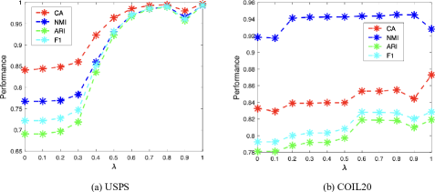
Figure 2: CA, NMI, ARI and F1 score of the proposed CCSC with respect to $\lambda$ on the USPS and COIL20 datasets.

5.2.2 Affinity graphs analysis

To gain a visual understanding of the advantages of our proposed FLNNSC, we plot the affinity graphs of all compared subspace clustering algorithms, as depicted in Figure 3. The figures reveal that many of the compared subspace clustering methods exhibit issues with unclear block-diagonal structures or noisy off-block-diagonal components. For instance, Figures 3(a), (d), (e), (g), and (h) clearly show the presence of noisy off-block-diagonal components, while Figure 3(b) illustrates an unclear block-diagonal structure. In contrast, Figure 3(l) highlights the distinct block-diagonal structure of our proposed FLNNSC algorithm, along with its off-block-diagonal components appearing less noisy, which is attributed to the eventual desirable clustering performance.

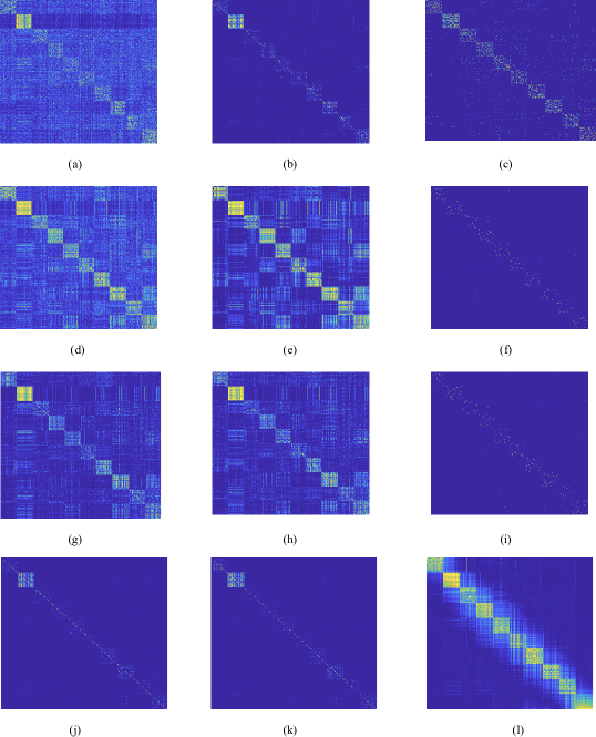
Figure 3: Affinity graphs produced by (a) SSC, (b) LRR, (c) LRSC, (d) NSC, (e) SMR, (f) KSSC, (g) LSR1, (h) LSR2, (i) KTRR, (j) BDR-B, (k) BDR-Z, (l) FLNNSC on the USPS.

5.2.3 Parameter sensitivity and convergence analysis

1) Parameter sensitivity analysis: In order to investigate the sensitivity of parameters in the FLNNSC algorithm, we analyze the influences of the parameters $\alpha$ and $\beta$. By varying these parameters over a range of values, we examine the variability of FLNNSC. Specifically, we set $\alpha$ and $\beta$ to vary from $10^{-4}$ to $10^{4}$. The experimental results are depicted in Figure 4.

On the Extended Yale B dataset, we observe that the parameter $\alpha$, when chosen within the range $[10^{-4},...,1]$, exhibits little influence on the algorithm’s performance. However, when $\alpha$ is set to be larger than 1, the clustering accuracy experiences significant variations. In contrast, FLNNSC shows little sensitivity to the parameter $\beta$ when its value is chosen within small values. On the USPS dataset, the selection of $\alpha$ has no obvious effects in terms of CA and NMI. However, FLNNSC demonstrates sensitivity to large values of $\beta$. Similarly, on the COIL20 dataset, we find that FLNNSC is not sensitive to the selection of $\alpha$, but it is sensitive to large values of $\beta$.

Based on our observations, we recommend choosing small values for $\beta$ to achieve better clustering performance in FLNNSC.

2) Convergence analysis: We conduct an experiment analysis to examine the convergence behavior of the proposed algorithm, utilizing the metric $\lVert\mathbf{Z}_{k}-\mathbf{Z}_{k-1}\rVert^{2}_{F}$, as shown in Figure 5. The obtained results demonstrate that the proposed FLNNSC algorithm exhibits rapid convergence across all three datasets, reaching a steady-state in a remarkably short period.

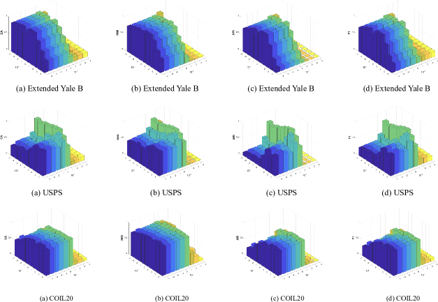
Figure 4: CA, NMI, ARI and F1 score with different $\alpha$ and $\beta$ combinations on the Extended Yale B (10 subjects), USPS and COIL20 datasets.

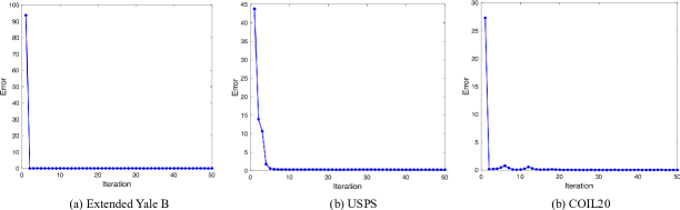
Figure 5: Convergence analysis on the Extended Yale B, USPS and COIL20 datasets.

5.2.4 Execution time analysis

In order to validate the efficiency of our method, we choose two benchmark methods for comparison: NSC and BDR. We select NSC for comparison as our method is developed in response to the limitations inherent in this particular approach. On the other hand, BDR is selected as it is a well-established baseline method known for its impressive performance across a variety of datasets. Figure 6 shows the comparison results of execution time on different datasets. It is seen that as the number of clusters increases, our method consistently outperforms both NSC and BDR in terms of execution time, thereby validating the efficiency of our proposed method.

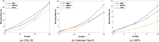
Figure 6: Comparison of execution time on different datasets.

5.3 Discussion

In subspace clustering, when the data exhibits evident nonlinearity characteristics, the combination method, i.e., CCSC, shows comparable clustering performance to FLNNSC under the optimal parameter settings. However, if the data also exhibits significant linear characteristics that cannot be ignored, CCSC outperforms FLNNSC due to its ability to dynamically adjust the balance between linear and nonlinear representations. Moreover, the proposed FLNNSC algorithm, using a functional link neural network for nonlinear representation, has higher computational efficiency compared to traditional neural network-based subspace clustering methods. Remarkably, to enhance the capacity for capturing the data’s nonlinearity, one can employ a higher-order functional expansion for FLNN. This may lead to performance improvements, but this enhancement introduces a trade-off by increasing computational intricacy.

6 Conclusions

We proposed a novel nonlinear subspace clustering method named as FLNNSC in this paper. By utilizing a single-layer FLNN with remarkable nonlinearity approximation capability, FLNNSC demonstrates the ability to exploit the nonlinear features of data, resulting in enhanced clustering performance. Moreover, the proposed FLNNSC algorithm was regularized to enable the grouping effect. To exploit both linear and nonlinear characteristics, we further introduced the CCSC algorithm, which dynamically adjusts the balance between linear and nonlinear representations via the combination parameter. Experiments on benchmark datasets have shown that our methods outperform several advanced subspace clustering methods. Additionally, affinity graph results have highlighted the grouping effect of FLNNSC. We conducted a parameter sensitivity analysis, yielding valuable suggestions for parameter selection. Furthermore, we empirically demonstrated the rapid convergence behavior of FLNNSC.

References

- [1] R. Vidal, Subspace clustering, IEEE Signal Process. Mag. 28 (2) (2011) 52–68.
- [2] J. Tang, Q. Yi, S. Fu, Y. Tian, Incomplete multi-view learning: Review, analysis, and prospects, Applied Soft Computing (2024) 111278.
- [3] E. Elhamifar, R. Vidal, Sparse subspace clustering: Algorithm, theory, and applications, IEEE Trans. Pattern Anal. Mach. Intell. 35 (11) (2013) 2765–2781.
- [4] L. Cao, L. Shi, J. Wang, Z. Yang, B. Chen, Robust subspace clustering by logarithmic hyperbolic cosine function, IEEE Signal Process. Lett. 30 (2023) 508–512.
- [5] G. Liu, Z. Lin, S. Yan, J. Sun, Y. Yu, Y. Ma, Robust recovery of subspace structures by low-rank representation, IEEE Trans. Pattern Anal. Mach. Intell. 35 (1) (2012) 171–184.
- [6] P. Favaro, R. Vidal, A. Ravichandran, A closed form solution to robust subspace estimation and clustering, in: Proceedings of the IEEE Conference on Computer Vision and Pattern Recognition, 2011, pp. 1801–1807.
- [7] G. Liu, Z. Lin, Y. Yu, Robust subspace segmentation by low-rank representation, in: Proceedings of the 27th International Conference on Machine Learning, 2010, pp. 663–670.
- [8] Y. Qin, X. Zhang, L. Shen, G. Feng, Maximum block energy guided robust subspace clustering, IEEE Trans. Pattern Anal. Mach. Intell. 45 (2) (2022) 2652–2659.
- [9] C. Lu, J. Feng, Z. Lin, T. Mei, S. Yan, Subspace clustering by block diagonal representation, IEEE Trans. Pattern Anal. Mach. Intell. 41 (2) (2018) 487–501.
- [10] V. M. Patel, H. Van Nguyen, R. Vidal, Latent space sparse subspace clustering, in: Proceedings of the IEEE International Conference on Computer Vision, 2013, pp. 225–232.
- [11] R. Vidal, Y. Ma, S. Sastry, Generalized principal component analysis (GPCA), IEEE Trans. Pattern Anal. Mach. Intell. 27 (12) (2005) 1945–1959.
- [12] J. Ho, M.-H. Yang, J. Lim, K.-C. Lee, D. Kriegman, Clustering appearances of objects under varying illumination conditions, in: Proceedings of the IEEE Conference on Computer Vision and Pattern Recognition, 2003, pp. 11–18.
- [13] M. E. Tipping, C. M. Bishop, Mixtures of probabilistic principal component analyzers, Neural Comput. 11 (2) (1999) 443–482.
- [14] S. Rao, R. Tron, R. Vidal, Y. Ma, Motion segmentation in the presence of outlying, incomplete, or corrupted trajectories, IEEE Trans. Pattern Anal. Mach. Intell. 32 (10) (2009) 1832–1845.
- [15] C. Li, C. You, R. Vidal, Structured sparse subspace clustering: A joint affinity learning and subspace clustering framework, IEEE Trans. Image Process. 26 (6) (2017) 2988–3001.
- [16] J. Liu, Y. Chen, J. Zhang, Z. Xu, Enhancing low-rank subspace clustering by manifold regularization, IEEE Trans. Image Process. 23 (9) (2014) 4022–4030.
- [17] J. Wang, D. Shi, D. Cheng, Y. Zhang, J. Gao, Lrsr: low-rank-sparse representation for subspace clustering, Neurocomputing 214 (2016) 1026–1037.
- [18] M. Brbić, I. Kopriva, -motivated low-rank sparse subspace clustering, IEEE Trans. Cybern. 50 (4) (2018) 1711–1725.
- [19] X. Zhu, S. Zhang, Y. Li, J. Zhang, L. Yang, Y. Fang, Low-rank sparse subspace for spectral clustering, IEEE Trans. Knowl. Data Eng. 31 (8) (2018) 1532–1543.
- [20] C. Lu, H. Min, Z. Zhao, L. Zhu, D. Huang, S. Yan, Robust and efficient subspace segmentation via least squares regression, in: Proceedings of the 12th European Conference on Computer Vision, 2012, pp. 347–360.
- [21] C. Lu, J. Feng, Z. Lin, S. Yan, Correlation adaptive subspace segmentation by trace lasso, in: Proceedings of the IEEE International Conference on Computer Vision, 2013, pp. 1345–1352.
- [22] H. Hu, Z. Lin, J. Feng, J. Zhou, Smooth representation clustering, in: Proceedings of the IEEE Conference on Computer Vision and Pattern Recognition, 2014, pp. 3834–3841.
- [23] L. Shi, H. Zhao, Y. Zakharov, An improved variable kernel width for maximum correntropy criterion algorithm, IEEE Trans. Circuits Syst. II 67 (7) (2018) 1339–1343.
- [24] L. Shi, L. Shen, B. Chen, An efficient parameter optimization of maximum correntropy criterion, IEEE Signal Process. Lett. 30 (2023) 538–542.
- [25] R. He, Y. Zhang, Z. Sun, Q. Yin, Robust subspace clustering with complex noise, IEEE Trans. Image Process. 24 (11) (2015) 4001–4013.
- [26] L. Guo, X. Zhang, Z. Liu, Q. Wang, J. Zhou, Correntropy metric-based robust low-rank subspace clustering for motion segmentation, Int. J. Mach. Learn. Cybern. 13 (5) (2022) 1425–1440.
- [27] X. Zhang, B. Chen, H. Sun, Z. Liu, Z. Ren, Y. Li, Robust low-rank kernel subspace clustering based on the schatten p-norm and correntropy, IEEE Trans. Knowl. Data Eng. 32 (12) (2019) 2426–2437.
- [28] V. M. Patel, R. Vidal, Kernel sparse subspace clustering, in: IEEE International Conference on Image Processing, IEEE, 2014, pp. 2849–2853.
- [29] M. Yin, Y. Guo, J. Gao, Z. He, S. Xie, Kernel sparse subspace clustering on symmetric positive definite manifolds, in: Proceedings of the IEEE conference on Computer Vision and Pattern Recognition, 2016, pp. 5157–5164.
- [30] C. Yang, Z. Ren, Q. Sun, M. Wu, M. Yin, Y. Sun, Joint correntropy metric weighting and block diagonal regularizer for robust multiple kernel subspace clustering, Inf. Sci. 500 (2019) 48–66.
- [31] L. Zhen, D. Peng, W. Wang, X. Yao, Kernel truncated regression representation for robust subspace clustering, Inf. Sci. 524 (2020) 59–76.
- [32] Z. Wang, J. Liu, Consensus kernel subspace clustering based on coefficient discriminant information, Applied Soft Computing 113 (2021) 107987.
- [33] Z. Kang, L. Wen, W. Chen, Z. Xu, Low-rank kernel learning for graph-based clustering, Knowl.-Based Syst. 163 (2019) 510–517.
- [34] X. Zhang, X. Xue, H. Sun, Z. Liu, L. Guo, X. Guo, Robust multiple kernel subspace clustering with block diagonal representation and low-rank consensus kernel, Knowl.-Based Syst. 227 (2021) 107243.
- [35] M. Sun, S. Wang, P. Zhang, X. Liu, X. Guo, S. Zhou, E. Zhu, Projective multiple kernel subspace clustering, IEEE Trans. Multimedia 24 (2021) 2567–2579.
- [36] W. Zhu, J. Lu, J. Zhou, Nonlinear subspace clustering for image clustering, Pattern Recognit. Lett. 107 (2018) 131–136.
- [37] X. Peng, J. Feng, J. T. Zhou, Y. Lei, S. Yan, Deep subspace clustering, IEEE Trans. Neural Netw. Learn. Syst. 31 (12) (2020) 5509–5521.
- [38] P. Ji, T. Zhang, H. Li, M. Salzmann, I. Reid, Deep subspace clustering networks, in: Advances in Neural Information Processing Systems, 2017, pp. 24–33.
- [39] J. C. Patra, A. C. Kot, Nonlinear dynamic system identification using chebyshev functional link artificial neural networks, IEEE Trans. Syst., Man, Cybern. B 32 (4) (2002) 505–511.
- [40] L. Lu, Y. Yu, X. Yang, W. Wu, Time delay chebyshev functional link artificial neural network, Neurocomputing 329 (2019) 153–164.
- [41] K. Yin, Y. Pu, L. Lu, Combination of fractional flann filters for solving the van der pol-duffing oscillator, Neurocomputing 399 (2020) 183–192.
- [42] S. Boyd, N. Parikh, E. Chu, B. Peleato, J. Eckstein, et al., Distributed optimization and statistical learning via the alternating direction method of multipliers, Found. Trends Mach. Learn. 3 (1) (2011) 1–122.
- [43] J. Wang, X. Wang, F. Tian, C. H. Liu, H. Yu, Constrained low-rank representation for robust subspace clustering, IEEE Trans. Cybern. 47 (12) (2016) 4534–4546.
- [44] J. Yang, J. Liang, K. Wang, P. L. Rosin, M.-H. Yang, Subspace clustering via good neighbors, IEEE Trans. Pattern Anal. Mach. Intell. 42 (6) (2019) 1537–1544.
- [45] R. Vidal, P. Favaro, Low rank subspace clustering (LRSC), Pattern Recognit. Lett. 43 (2014) 47–61.