Non-minimal Derivative Coupling Theories Compatible with GW170817

Abstract

In this work we aim to revive the interest for non-minimal derivative coupling theories of gravity, in light of the GW170817 event. These theories include a string motivated non-minimal kinetic term for the scalar field of the form $\sim\xi(\phi)G^{\mu\nu}\partial_{\mu}\phi\partial_{\nu}\phi$ and predict that the primordial tensor perturbations have a speed that it is distinct from the speed of light. Due to the fact that the Universe is classical during and in the post-inflationary epoch, there is no fundamental reason for the graviton to change its mass, the GW170817 event severely constrained these theories. We analyze and formalize the inflationary phenomenology of these theories, using both the latest Planck data and the GW170817 event data to constrain these theories. Due to the fact that there is no constraint in the choice of the scalar potential and the non-minimal coupling function, we provide several classes of viable models, using convenient forms of the minimal coupling function in terms of the scalar potential, aiming for analyticity, and we discuss the advantages and disadvantages of each viable model.

I Introduction

Modern cosmology is rendered a precision science, due to the astonishing amounts of observational data available nowadays. Thus, theoretical models of the Universe are currently being severely scrutinized, and the years to follow are promising regarding cosmological theories. The year that utterly changed the theoretical perception in theoretical cosmology was 2017 with the remarkable GW170817 event from the LIGO-Virgo collaboration [1, 2, 3, 4], which was astonishing due to a fact that apart from the gravitational wave detected by the merging neutron stars, a kilonova was also detected. This event changed our theoretical perception of our Universe, since massive gravity theories of inflation were excluded or severely constrained [5, 6, 7, 8]. The GW170817 event started the chorus of groundbreaking observations, continued in 2023 with the NANOGrav detection of a stochastic gravitational wave background [9]. These collaborations, in conjunction with the future observations that are highly anticipated, coming from gravitational wave experiments like LISA [10, 11], BBO [12, 13] and DECIGO [14, 15], are expected to further enlarge our knowledge about astrophysical and cosmological theories. Regarding the GW170817 event, as we mentioned, it severely constrained theories that predict gravitational waves with speed smaller than that of light. This is a late-time event though, thus one might claim that the gravitational wave speed at early times could be different from that of light. However, the primordial gravitational waves, are basically classical tensor perturbations of a classical spacetime, describing a classical post-Planck Universe. Indeed, when the inflationary era is believed to have started, the Universe was four dimensional and free from severe quantum effects. The quantum effects may have their imprints on the inflationary Lagrangian, however, no direct quantum effect is expected when the inflationary era started, and beyond that. Thus, from a particle physics viewpoint, there is no fundamental inherent mechanism that can effectively change the graviton mass during and in the post-inflationary era. Thus the primordial gravitational waves should also be constrained in the same manner as ordinary late-time gravitational waves from the GW170817 event. Motivated by this aspect of research, in this work we shall thoroughly study a class of theories which was affected by the GW170817 event, the non-minimal derivative theories of gravity which include non-minimal kinetic coupling terms of the form $\sim\xi(\phi)G^{\mu\nu}\partial_{\mu}\phi\partial_{\nu}\phi$. These theories constitute an important subclass of Horndeski theories [16, 17, 18, 19, 20, 21, 22, 23, 24, 25, 26, 27, 28, 29], and were thoroughly studied in the pre-GW170817 epoch [30, 31, 32, 33, 34, 35, 36, 37, 38, 39, 40, 41, 42, 43, 44, 45, 46, 47, 48], see also [49] where the same non-minimal derivative coupling term is suitably chosen in order to have constant gravitational wave speed and equal to the light speed and also to solve the $H_{0}$-tension, and also Ref. [50] in which case the non-minimal derivative coupling is used for inflation but in a way that it becomes negligible after inflation exit, and thus passing GW170817 constraints easily. In this work we aim to revive these theories, by also including the constraints from the GW170817 event in their inflationary phenomenological analysis. A similar approach was performed in Refs. [51, 52, 53] for Horndeski theories. Non-minimal derivative theories are basically string inspired theories, which take into account imprints of a more fundamental theory on the inflationary Lagrangian, and serve as an important path of the classical theory towards to the more fundamental quantum theory. Getting to the details of model building of the non-minimal derivative kinetic coupling theories, the scalar field potential and the kinetic coupling scalar function are unconstrained from a theoretical point of view, so in principle any choice for these functions can be examined regarding the phenomenological viability of the theory. In this work we aim to thoroughly formalize these theories and study their inflationary phenomenology in a concrete and self-consistent way. We present various classes of solutions and choices for the non-minimal kinetic coupling function $\xi(\phi)$ and we examine the inflationary phenomenology of the theory, confronting the models with the latest Planck data, and also discussing the attributes and drawbacks of each model.

This paper is organized as follows: In section II we present the formalism of non-minimal derivative kinetic coupling theories, we extract analytic forms for the gravitational wave speed of tensor perturbations, the slow-roll indices, the observational indices and the amplitude of the scalar perturbations and we also provide all the necessary theoretical tools and constraints that we will enable us to extract a viable phenomenology from these theories. In section III we study several classes of viable theoretical models and we discuss the advantages and disadvantages of each model. Finally, the conclusions follow at the end of the article.

II Non-minimal Derivative Coupling Theories Theoretical Framework and Compatibility with GW170817 Constraints

In principle, the non-minimal derivative coupling theories constitute a string-corrected scalar theory, with leading order corrections in the Regge slope, without including Einstein-Gauss-Bonnet terms and higher derivatives of the scalar field too [30, 54]. The gravitational action reads,

$$\centering\mathcal{S}=\int{d^{4}x\sqrt{-g}\left(\frac{R}{2\kappa^{2}}-\frac{1}{2}g^{\mu\nu}\partial_{\mu}\phi\partial_{\nu}\phi-V(\phi)-c\xi(\phi)G^{\mu\nu}\partial_{\mu}\phi\partial_{\nu}\phi\right)}\,,\@add@centering$$ (1)

with $R$ denoting as usual the Ricci scalar, $g$ stands for the determinant of the metric tensor, $\kappa=\frac{1}{M_{P}}$ where $M_{P}$ is the reduced Planck mass, $V(\phi)$ is the scalar field potential, and $\xi(\phi)$ is the non-minimal derivative coupling function of the kinetic coupling term $\sim c\,\xi(\phi)G^{\mu\nu}\partial_{\mu}\phi\partial_{\nu}\phi$, where $G^{\mu\nu}$ denotes the Einstein tensor $G^{\mu\nu}=R^{\mu\nu}-\frac{1}{2}g^{\mu\nu}R$, and $c$ is an arbitrary parameter with mass dimensions $[M]^{-2}$.

With regard to the background metric, we shall consider a flat Friedman-Lemaitre-Robertson-Walker (FLRW) background with line element,

$$\centering ds^{2}=-dt^{2}+a^{2}\delta_{ij}dx^{i}dx^{j}\,,\@add@centering$$ (2)

with $a(t)$ denoting the scale factor of the Universe. In this type of theories, the propagation speed of the tensor perturbations, or equivalently the speed of the primordial gravitational waves, has the following form [30],

$$\centering c_{T}^{2}=1-\frac{Q_{f}}{2Q_{t}}\,,\@add@centering$$ (3)

with the term $Q_{f}$ being equal to,

$$Q_{f}=4c\xi\dot{\phi}^{2}\,,$$ (4)

where the “dot” denotes differentiation with respect to the cosmic time hereafter. Moreover, $Q_{t}$ in Eq. (4) stands for $Q_{t}=\frac{1}{\kappa^{2}}+c\xi\dot{\phi}^{2}$. Thus the primordial gravitational wave speed takes the form,

$$\centering c_{T}^{2}=1-\frac{2c\kappa^{2}\xi\dot{\phi}^{2}}{1+c\kappa^{2}\xi\dot{\phi}^{2}}\,.\@add@centering$$ (5)

Thus in order to comply with the striking GW170817 event which rules out massive graviton theories, it is vital that the following constraint is satisfied at first horizon crossing during inflation, but also for all the subsequent eras,

$$\kappa^{2}c\xi\dot{\phi}^{2}\ll 1\,,$$ (6)

and specifically the term $\kappa^{2}c\xi\dot{\phi}^{2}$ must be sufficiently smaller than unity in order for the GW170817 experimental constraint to be satisfied, which is,

$$\left|c_{T}^{2}-1\right|<6\times 10^{-15}\,,$$ (7)

in natural units. Regarding the constraint (6), as we mentioned, it has to be satisfied for all the post-first horizon crossing eras, and this is a necessity since there is no fundamental particle physics reason for the graviton to change its mass in the inflationary and post inflationary era, because the inflationary era and all the subsequent eras, are basically classical eras of our Universe, hence no big change in the propagating mass of the particles is expected. The gravitational field equations can be obtained by varying the gravitational action (1), with respect to the metric tensor and with respect to the scalar field, so we get the Friedmann equation,

$$\centering\frac{3H^{2}}{\kappa^{2}}=\frac{1}{2}\dot{\phi}^{2}-9c\,\xi H^{2}\dot{\phi}^{2}\,,\@add@centering$$ (8)

the Raychaudhuri equation,

$$\centering-\frac{2\dot{H}}{\kappa^{2}}=\dot{\phi}^{2}-8H^{2}(\ddot{\xi}-H\dot{\xi})+c\left(2\xi(\dot{H}-3H^{2})\dot{\phi}^{2}+4H\xi\dot{\phi}\ddot{\phi}+2H\dot{\xi}\dot{\phi}^{2}\right)\,,\@add@centering$$ (9)

and the scalar field generalized Klein-Gordon equation,

$$\centering\ddot{\phi}+3H\dot{\phi}+V^{\prime}+6c\left(H^{2}(\dot{\xi}\dot{H}+2\xi\ddot{\phi})+2H(2\dot{H}+3H^{2})\xi\dot{\phi}\right)=0\,.\@add@centering$$ (10)

The field equations are coupled differential equations with quite involved form, and it is understandable that an analytic solution is not easy to be obtained. However, several simplifications may be applied during the inflationary era, such as the slow-roll approximation for the scalar field and the inflationary conditions for the Hubble rate, and specifically the following approximations,

$$\centering\dot{H}\@add@centering \ll H^{2} \frac{1}{2}\dot{\phi}^{2} \ll V \ddot{\phi} \ll H\dot{\phi}\,.$$ (11)

Also we must take into account the condition of Eq. (6), which is a imposed inherent necessity for the viability and compatibility of the theory with the GW170817 event, thus we must also take into account that $\kappa^{2}c\,\xi\dot{\phi}^{2}\ll 1$. This term, namely $9c\,\xi H^{2}\dot{\phi}^{2}$ enters the Friedmann equation and thus it is not dominant at leading order, and also $\dot{\phi}^{2}$ must also be subdominant, hence only the scalar potential survives, therefore the Friedmann equation becomes,

$$\centering H^{2}\simeq\frac{\kappa^{2}V}{3}\,.\@add@centering$$ (12)

In the end, the approximations we made, must be checked explicitly, namely,

$$c\,\xi\dot{\phi}^{2}\ll V,\,\,\,\dot{\phi}^{2}\ll V\,,$$ (13)

however these two are not additional constraints in the theory, imposed by hand, but these stem from the natural requirements that the gravitational wave speed is equal to that of light and also that the slow-roll approximation holds for the scalar field. For consistency though, we will validate these constraints for any viable model we shall present. Accordingly, by using the slow-roll and inflationary constraints, the Raychaudhuri equations read,

$$\centering-\dot{H}=\frac{\kappa^{2}\dot{\phi}^{2}}{2}-3c\kappa^{2}\xi H^{2}\dot{\phi}^{2}\,,\@add@centering$$ (14)

or equivalently,

$$\centering-\dot{H}=\frac{\kappa^{2}\dot{\phi}^{2}}{2}\left(1-6c\,\xi H^{2}\right)\,.\@add@centering$$ (15)

Accordingly, by using the slow-roll and inflationary constraints (11), the modified Klein-Gordon equation reads,

$$\centering V^{\prime}+3H\dot{\phi}+36c\xi\dot{\phi}H^{3}\simeq 0\,,\@add@centering$$ (16)

which can be rewritten,

$$\dot{\phi}=-\frac{V^{\prime}}{3H\left(1+12c\,\xi H^{2}\right)}\,.$$ (17)

From the final form of the Raychaudhuri equation (15) and of the modified Klein-Gordon equation (17), it is obvious that the term $\sim c\,\xi H^{2}$ enters both equations and if this dominant compared to unity, then both the Raychaudhuri equation and the modified Klein-Gordon equation can be simplified. We shall make this approximation in the following and also we shall consider the generalized formulas. So in the following we shall consider two classes of non-minimal derivative couplings models, one that the following constraint holds true,

$$c\,\xi H^{2}\gg 1\,,$$ (18)

in which case, the Raychaudhuri and the modified Klein-Gordon equations take the form,

$$\centering-\dot{H}=-3c\,\xi H^{2}\kappa^{2}\dot{\phi}^{2}\,,\@add@centering$$ (19)

$$\dot{\phi}=-\frac{V^{\prime}}{36c\,\xi H^{3}}\,,$$ (20)

and general models which do not respect the constraint (18) and thus the Raychaudhuri and the Klein-Gordon equations are given in Eqs. (15) and (17) respectively. We shall refer to the models that satisfy the constraint (18) as “constrained models”. Now let us present the slow-roll indices of inflation, the observational indices of inflation and the relation that yields the $e$-foldings number for the non-minimal derivative coupling theories of gravity, for both the constrained models and the unconstrained models. The slow-roll indices for the non-minimal derivative coupling theories have the general form [30],

$$\centering\epsilon_{1}\@add@centering =-\frac{\dot{H}}{H^{2}} \epsilon_{2} =\frac{\ddot{\phi}}{H\dot{\phi}} \epsilon_{3} =0 \epsilon_{4} =\frac{\dot{E}}{2HE} \epsilon_{5} =\frac{Q_{a}}{2HQ_{t}} \epsilon_{6} =\frac{\dot{Q}_{t}}{2HQ_{t}}\,,$$ (21)

where $Q_{a}=4c\,\xi H\dot{\phi}^{2}$, $Q_{b}=2c\,\xi\dot{\phi}^{2}$, $E=\frac{1}{(\kappa\dot{\phi})^{2}}\left(\dot{\phi}^{2}+\frac{3Q_{a}^{2}}{2Q_{t}}+Q_{c}\right)$, $Q_{c}=-6c\,\xi\dot{\phi}^{2}H^{2}$, $Q_{d}=-4c\,\xi\dot{\phi}^{2}\dot{H}$, $Q_{e}=4c\dot{\phi}\left(\dot{\xi}\dot{\phi}+2\xi\ddot{\phi}-2\xi\dot{\phi}H\right)$, $Q_{f}=4c\,\xi\dot{\phi}^{2}$ and recall that $Q_{t}=\frac{1}{\kappa^{2}}+\frac{Q_{b}}{2}$. The observational indices of inflation in terms of the slow-roll indices have the following form,

$$n_{\mathcal{S}}=1+\frac{2(-2\epsilon_{1}-\epsilon_{2}-\epsilon_{4})}{1-\epsilon_{1}}\,,$$ (22)

regarding the spectral index of the scalar primordial curvature perturbations, while the tensor-to-scalar ratio has the form,

$$r=\left|\frac{16\left(c_{A}^{3}\left(\epsilon_{1}-\frac{1}{4}\kappa^{2}\left(\frac{2Q_{c}+Q_{d}}{H^{2}}-\frac{Q_{e}}{H}+Q_{f}\right)\right)\right)}{c_{T}^{3}\left(\frac{\kappa^{2}Q_{b}}{2}+1\right)}\right|\,,$$ (23)

where $c_{A}$ is the sound speed of the scalar perturbations, defined as,

$$c_{A}=\sqrt{\frac{\frac{Q_{a}Q_{e}}{\frac{2}{\kappa^{2}}+Q_{b}}+Q_{f}\left(\frac{Q_{a}}{\frac{2}{\kappa^{2}}+Q_{b}}\right)^{2}+Q_{d}}{\dot{\phi}^{2}+\frac{3Q_{a}^{2}}{\frac{2}{\kappa^{2}}+Q_{b}}+Q_{c}}+1}\,,$$ (24)

and also $c_{T}$ is the speed of tensor perturbations defined in Eq. (5). Also the tensor spectral index is given in terms of the slow-roll parameters as follows,

$$n_{\mathcal{T}}=-2\frac{\left(\epsilon_{1}+\epsilon_{6}\right)}{1-\epsilon_{1}}\,.$$ (25)

Let us now express the $e$-foldings number in terms of the potential and its derivatives. The definition of the $e$-foldings number is,

$$\centering N=\int_{t_{i}}^{t_{f}}{Hdt}=\int_{\phi_{i}}^{\phi_{f}}\frac{H}{\dot{\phi}}d\phi\,,\@add@centering$$ (26)

where $\phi_{i}$ and $\phi_{f}$ are the scalar field values at the beginning (first horizon crossing) and the end of the inflationary era. The value of the scalar field at the end of the inflationary era can be obtained by solving $|\epsilon_{1}|\sim\mathcal{O}(1)$, while by solving Eq. (26) with respect to $\phi_{i}$ one may obtain the value of the scalar field at first horizon crossing, namely $\phi_{i}$. By using Eqs. (12) and (17) we get,

$$\centering N=\int_{t_{i}}^{t_{f}}{Hdt}=\int_{\phi_{f}}^{\phi_{i}}\frac{\kappa^{2}V\left(1+4c\kappa^{2}V\xi\right)}{V^{\prime}}d\phi\,,\@add@centering$$ (27)

for the case of the unconstrained, while in the case of the constrained models which satisfy the constraint (18), the $e$-foldings number is given by the following relation,

$$\centering N=\int_{t_{i}}^{t_{f}}{Hdt}=4c\kappa^{4}\int_{\phi_{f}}^{\phi_{i}}\frac{\xi V^{2}}{V^{\prime}}d\phi\,.\@add@centering$$ (28)

Before closing this section, let us also mention another important constraint which needs to be taken into account in order to provide a viable phenomenology, related with the amplitude of the scalar perturbations $\mathcal{P}_{\zeta}(k_{*})$, defined as,

$$\mathcal{P}_{\zeta}(k_{*})=\frac{k_{*}^{3}}{2\pi^{2}}P_{\zeta}(k_{*})$$ (29)

which must be evaluated at first horizon crossing during the inflationary era, denoted as $k_{*}$, known as the pivot scale $k_{*}=0.05$Mpc^-1, and is highly relevant to the CMB observations. The latest Planck data [55] constrain the amplitude of the scalar perturbations to be $\mathcal{P}_{\zeta}(k_{*})=2.196^{+0.051}_{-0.06}\times 10^{-9}$, when this is evaluated at the CMB pivot scale. The scalar amplitude for the scalar perturbations $\mathcal{P}_{\zeta}(k)$ in terms of the two point function for the curvature perturbations $\zeta(k)$ through $P_{\zeta}(k)$ which appears in Eq. (29) is,

$$\langle\zeta(k)\zeta(k^{\prime})\rangle=(2\pi)^{3}\delta^{3}(k-k^{\prime})P_{\zeta}(k)\,.$$ (30)

For the non-minimal derivative coupling theories, the amplitude $\mathcal{P}_{\zeta}(k_{*})$ in the slow-roll approximation is [30],

$$\mathcal{P}_{\zeta}(k)=\left(\frac{k\left((-2\epsilon_{1}-\epsilon_{2}-\epsilon_{4})\left(0.57\,+\log\left(\left|k\eta\right|\right)-2+\log(2)\right)-\epsilon_{1}+1\right)}{(2\pi)\left(zc_{A}^{\frac{4-n_{\mathcal{S}}}{2}}\right)}\right)^{2}\,,$$ (31)

evaluated at first horizon crossing, with $z=\frac{a\dot{\phi}\sqrt{\frac{E(\phi)}{\frac{1}{\kappa^{2}}}}}{H(\epsilon_{5}+1)}$ at first horizon crossing, and in addition the conformal time at first horizon crossing is $\eta=-\frac{1}{aH}\frac{1}{-\epsilon_{1}+1}$ [30]. In the following we shall also take this into account in order to generate viable phenomenologies of non-minimal derivative coupling theories.

III Phenomenology of Various Classes of Viable Models

In this section we shall thoroughly analyze the inflationary phenomenology of several classes of non-minimal derivative coupling theories, confronting the models with the Planck constraints. In principle, for the theories at hand, the scalar potential $V(\phi)$ and the scalar coupling function $\xi(\phi)$ are free to choose, since these are not fundamentally constrained, as in the case of constrained Einstein-Gauss-Bonnet gravity developed in Refs. [56, 57, 58]. Thus, we shall choose them freely, using convenient forms for their functional form which may lead to analytical results. We found several classes of models that may provide analytic results, and in many cases viable phenomenologies. We shall use the Planck units system in which

$$\kappa^{2}=\frac{1}{8\pi G}=\frac{1}{M_{P}^{2}}=1$$

for convenience. Also for each viable model presented, we shall verify explicitly that the slow-roll and any additional constraints that render the gravitational wave speed equal to that of light are satisfied. We start our analysis with the constrained models that satisfy the constraint of Eq. (18) and we continue with the unconstrained models.

III.1 Phenomenology of Constrained Models

Let us begin our analysis by studying the constrained models which must obey the constraint of Eq. (18). For these models, the Friedmann and Raychaudhuri equations are given in Eqs. (12) and (19) and the derivative of the scalar field is given by Eq. (20), while the $e$-foldings number is given by Eq. (28). Using these, in addition to Eqs. (21), (22), (23), (24) and (25), one may obtain study in detail the inflationary phenomenology of this class of models. As we mentioned earlier, there is no fundamental constraint that constrains the functional form of the scalar potential and of the scalar coupling function, thus these are free to choose and unrelated. Thus, we shall choose these in a way so that analytic expressions for the inflationary indices and for the rest of the parameters are obtained. In order to discover interesting classes of models, we shall quote here the analytic form of the first slow-roll index $\epsilon_{1}$, which is,

$$\epsilon_{1}=-\frac{V^{\prime}(\phi)^{2}}{16c\kappa^{4}\xi(\phi)V(\phi)^{3}}\,,$$ (32)

hence we quote here convenient choices for the coupling function $\xi(\phi)$ in Planck units:

$$\xi(\phi)=\frac{1}{V(\phi)}\,,$$ (33)

$$\xi(\phi)=\lambda V^{\prime}(\phi)^{2}\,,$$ (34)

$$\xi(\phi)=\frac{\lambda V^{\prime}(\phi)}{V(\phi)^{2}}\,,$$ (35)

$$\xi(\phi)=\frac{\lambda V^{\prime}(\phi)}{V(\phi)}\,,$$ (36)

$$\xi(\phi)=\frac{\lambda V^{\prime}(\phi)}{V(\phi)^{3}}\,,$$ (37)

From all the choices, the most interesting phenomenologically is the class of models (35). The classes of models (34), (36) and (37) do not yield viable results for a large number of freely chosen scalar potentials, and the main reason for this behavior is the final form of the gravitational wave speed, which can never be compatible with the GW170817 constraint of Eq. (7). Indeed for the models of the class (34), the gravitational wave speed has the form,

$$c_{T}^{2}=\frac{48c\lambda V(\phi)^{3}-1}{48c\lambda V(\phi)^{3}+1}\,,$$ (38)

and as it proves it is always of the order $\sim\mathcal{O}(10^{-3})$ for a large number of scalar potentials. Also regarding the class of models (36) the gravitational wave speed has the form,

$$c_{T}^{2}=\frac{48c\lambda V(\phi)^{2}-V^{\prime}(\phi)}{48c\lambda V(\phi)^{2}+V^{\prime}(\phi)}\,,$$ (39)

and as it proves in this case too, it is always of the order $\sim\mathcal{O}(10^{-3})$ for a large number of scalar potentials. Finally for the class of models (37) the gravitational wave speed has the form,

$$c_{T}^{2}=\frac{48c\lambda-V^{\prime}(\phi)}{48c\lambda+V^{\prime}(\phi)}\,,$$ (40)

and as it proves in this case too, it is always of the order $\sim\mathcal{O}(10^{-3})$ for a large number of scalar potentials. Hence, we shall analyze only the class of models (33) and (35). Among the two, the most interesting phenomenologically is the class (35) since we found a large number of scalar potentials that yield a viable phenomenology, so we start our analysis with this class of models. In this case, the first slow-roll index acquires a quite simplified form and it is equal to,

$$\epsilon_{1}=-\frac{V^{\prime}(\phi)}{16c\lambda V(\phi)}\,,$$ (41)

while the $e$-foldings number as a function of the final and initial scalar field values reads,

$$N=4c\lambda\phi_{f}-4c\lambda\phi_{i}\,,$$ (42)

and it is independent from the actual form of the potential, due to the choice of the scalar coupling function (34). The gravitational wave speed in this case has the form,

$$c_{T}^{2}=\frac{48c\lambda V(\phi)-V^{\prime}(\phi)}{48c\lambda V(\phi)+V^{\prime}(\phi)}\,.$$ (43)

Among the rest of the slow-roll indices of inflation and the observational indices, only the tensor spectral index has a simple form, which we quote here due to the importance of the tensor spectral index for the primordial gravitational waves,

$$n_{\mathcal{T}}=\frac{4V(\phi)\left(24c\lambda V^{\prime}(\phi)+V^{\prime\prime}(\phi)\right)-2V^{\prime}(\phi)^{2}}{\left(16c\lambda V(\phi)+V^{\prime}(\phi)\right)\left(48c\lambda V(\phi)+V^{\prime}(\phi)\right)}\,.$$ (44)

Now let us consider various scalar potentials and we study their inflationary phenomenology and consistency in detail. We start with the following potential,

$$V(\phi)=\frac{M}{1-\frac{d}{\phi}}\,,$$ (45)

in which case the scalar coupling function $\xi(\phi)$ reads,

$$\xi(\phi)=-\frac{d\lambda}{M\phi^{2}}\,,$$ (46)

so the first slow-roll index reads in this case,

$$\epsilon_{1}=-\frac{d}{16c\,d\lambda\phi-16c\lambda\phi^{2}}\,,$$ (47)

and thus by solving the equation $|\epsilon_{1}(\phi_{f})|=1$ we obtain the value of the scalar field at the end of inflation $\phi_{f}$ which is,

$$\phi_{f}=\frac{\sqrt{4c^{2}d^{2}\lambda^{2}+c\,d\lambda}+2c\,d\lambda}{4c\lambda}\,,$$ (48)

and from Eq. (42), the value of the scalar field at first horizon crossing is,

$$\phi_{i}=\frac{2c\,d\lambda+\sqrt{c\,d\lambda(4c\,d\lambda+1)}+N}{4c\lambda}\,.$$ (49)

Now a viable phenomenology is obtained for $N=61$ for various values of the free parameters, for example if we choose the free parameters of the model as follows $(c,d,M,\lambda)=(10^{25.5},10^{-21},1.46725\times 10^{-22},10^{-16.47})$, in which case, the spectral index of the scalar perturbations, the tensor-to-scalar ratio and the tensor spectral index take the values $n_{\mathcal{S}}=0.967162$, $r=4.57199\times 10^{-15}$ and $n_{\mathcal{T}}=-5.74661\times 10^{-16}$, thus the model is viable regarding the observational indices of inflation. Also in Fig. 1 we confront the model with the Planck likelihood curves, for $N=[50,65]$ and we can see that the model can be well fitted in the Planck data.

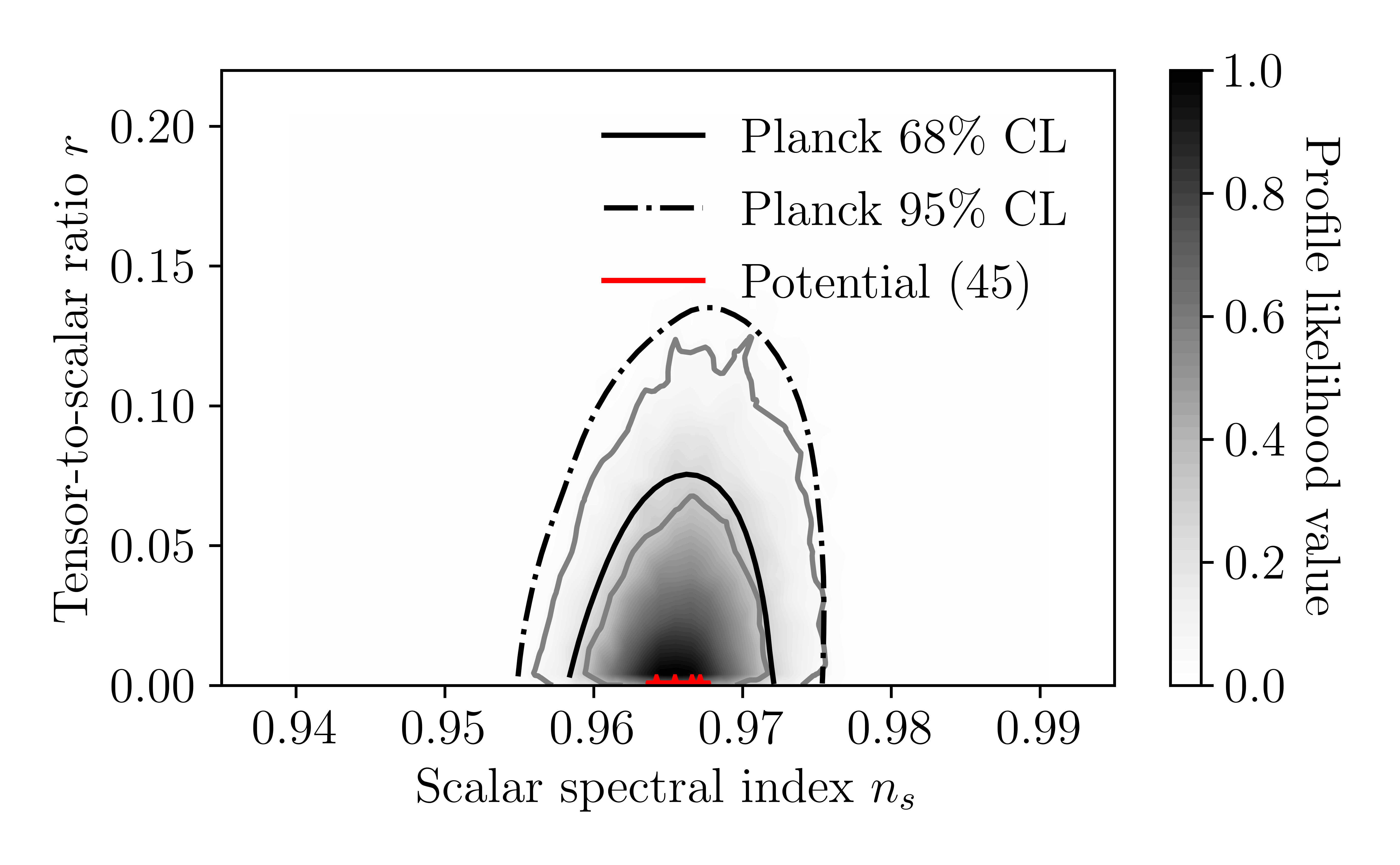
Figure 1: Marginalized curves of the Planck 2018 data and the model with potential $V(\phi)=\frac{M}{1-\frac{d}{\kappa\phi}}$ of Eq. (45) vs the Planck 2018 data (red curve), for $N=[50,65]$ and for $(c,d,M,\lambda)=(10^{25.5},10^{-21},1.46725\times 10^{-22},10^{-16.47})$.

Also the amplitude of the scalar perturbations for the model at hand for $(c,d,M,\lambda)=(10^{25.5},10^{-21},1.46725\times 10^{-22},10^{-16.47})$ is $\mathcal{P}_{\zeta}(k_{*})=2.196\times 10^{-9}$, and actually, the value of the parameter $M$ crucially affects only the amplitude of the scalar perturbations, since all the rest of the inflationary indices are independent of $M$. Now, for $(c,d,M,\lambda)=(10^{25.5},10^{-21},1.46725\times 10^{-22},10^{-16.47})$ the values of the scalar field at the beginning and the end of inflation are $(\phi_{i},\phi_{f})=(1.42088\times 10^{-8},2.41513\times 10^{-16})$, which are sub-Planckian values, thus the model is self-consistent. Also note that the singularity in the potential (45) is avoided because it may occur only for $\phi\sim d$, and the scalar field never reaches the values of $d$ we used, which is $d\sim 10^{-21}$. More importantly, we find that $c_{T}^{2}-1=1.92608\times 10^{-16}$ and also the model well satisfies the constraint (18), since we find that for $(c,d,M,\lambda)=(10^{25.5},10^{-21},1.46725\times 10^{-22},10^{-16.47})$, $c\,\xi H^{2}\sim\mathcal{O}(10^{4})$. Moreover, let us check whether the slow-roll approximations (11) and also the approximations of Eq. (13) hold true. As we found, for $(c,d,M,\lambda)=(10^{25.5},10^{-21},1.46725\times 10^{-22},10^{-16.47})$ we have $\dot{\phi}^{2}\sim\mathcal{O}(10^{-42})$, $c\,\xi\dot{\phi}^{2}\sim\mathcal{O}(10^{-38})$ and $V\sim\mathcal{O}(10^{-22})$, hence the model is self-consistent and well fitted within the Planck 2018 data. Let us also study the behavior of the gravitational wave speed as a function of the $e$-foldings number. Before that however, we need to note that the gravitational wave speed must satisfy the GW170817 constraints only at first horizon crossing, since after that and especially near the end of inflation, the slow-roll conditions are violated so it does not make much sense to use the expressions for the slow-roll indices and the other quantities we used in the previous section. However, for completeness, in Fig. 2 we present the behavior of the gravitational wave speed $c_{T}^{2}$. As it can be seen, it is equal to unity, but this should not be taken for granted, since the slow-roll assumptions are violated near the end of inflation and thus the expressions we used might not be applicable.

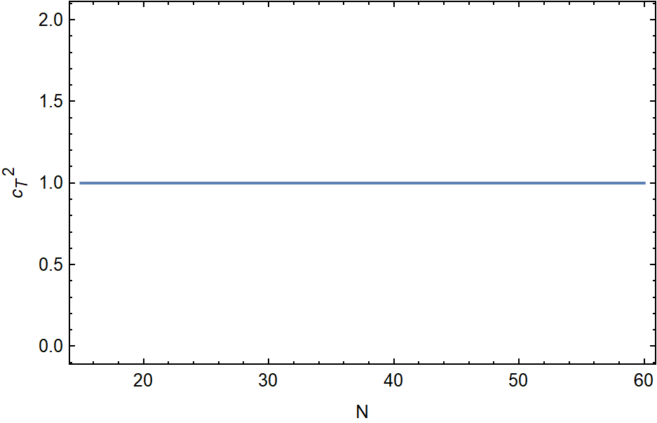
Figure 2: The gravitation wave speed $c_{T}^{2}$ for the model with potential $V(\phi)=\frac{M}{1-\frac{d}{\kappa\phi}}$ of Eq. (45) for $N=[0,60]$ and for $(c,d,M,\lambda)=(10^{25.5},10^{-21},1.46725\times 10^{-22},10^{-16.47})$.

Let us consider another viable potential at this point, in which case the potential is,

$$V(\phi)=M\left(1-\frac{d}{\phi}\right)^{1/100}\,,$$ (50)

in which case the scalar coupling function $\xi(\phi)$ reads,

$$\xi(\phi)=\frac{d\lambda}{100M\phi^{2}\left(1-\frac{d}{\phi}\right)^{101/100}}\,,$$ (51)

so the first slow-roll index reads in this case,

$$\epsilon_{1}=\frac{d}{1600c\,d\lambda\phi-1600c\lambda\phi^{2}}\,,$$ (52)

and thus by solving the equation $|\epsilon_{1}(\phi_{f})|=1$ we obtain the value of the scalar field at the end of inflation $\phi_{f}$ which is,

$$\phi_{f}=\frac{\sqrt{400c^{2}d^{2}\lambda^{2}-c\,d\lambda}+20c\,d\lambda}{40c\lambda}\,,$$ (53)

and from Eq. (42), the value of the scalar field at first horizon crossing is,

$$\phi_{i}=\frac{20c\,d\lambda+\sqrt{c\,d\lambda(400c\,d\lambda-1)}+10N}{40c\lambda}\,.$$ (54)

Now a viable phenomenology is obtained for $N=61$ for various values of the free parameters, for example if we choose the free parameters of the model as follows $(c,d,M,\lambda)=(10^{25.5},-10^{-21},1.48126\times 10^{-24},10^{-16.47})$, in which case, the spectral index of the scalar perturbations, the tensor-to-scalar ratio and the tensor spectral index take the values $n_{\mathcal{S}}=0.967466$, $r=4.57199\times 10^{-17}$ and $n_{\mathcal{T}}=-5.74661\times 10^{-18}$, thus the model is viable regarding the observational indices of inflation. Also in Fig. 3 we confront the model with the Planck likelihood curves, for $N=[50,65]$ and we can see that the model can be well fitted in the Planck data.

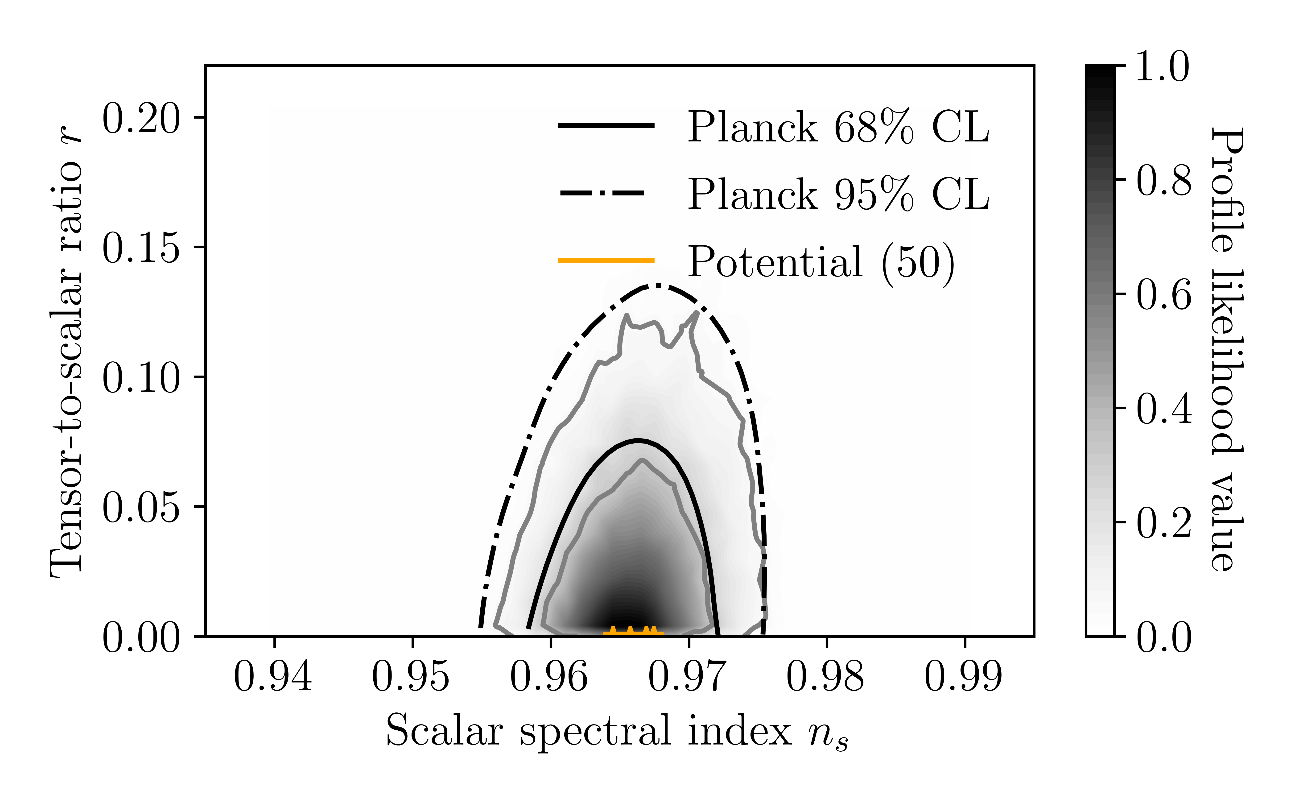
Figure 3: Marginalized curves of the Planck 2018 data and the model with potential $V(\phi)=M\left(1-\frac{d}{\kappa\phi}\right)^{1/100}$ of Eq. (50) vs the Planck 2018 data (yellow curve) for $N=[50,65]$ and $(c,d,M,\lambda)=(10^{25.5},-10^{-21},1.48126\times 10^{-24},10^{-16.47})$.

Also the amplitude of the scalar perturbations for the model at hand for $(c,d,M,\lambda)=(10^{25.5},-10^{-21},1.48126\times 10^{-24},10^{-16.47})$ is $\mathcal{P}_{\zeta}(k_{*})=2.196\times 10^{-9}$, and actually, the value of the parameter $M$ crucially affects only the amplitude of the scalar perturbations, since all the rest of the inflationary indices are independent of $M$. Now, for $(c,d,M,\lambda)=(10^{25.5},-10^{-21},1.48126\times 10^{-24},-10^{-16.47})$ the values of the scalar field at the beginning and the end of inflation are $(\phi_{i},\phi_{f})=(1.42088\times 10^{-8},2.41508\times 10^{-17})$, which are sub-Planckian values, hence the model is self-consistent. Also note that the singularity in the potential (50) is avoided because $d<0$ in this case. Also, we find that $c_{T}^{2}-1=1.92608\times 10^{-18}$ and in addition the model well satisfies the constraint (18), since we find that for $(c,d,M,\lambda)=(10^{25.5},-10^{-21},1.48126\times 10^{-24},10^{-16.47})$, $c\,\xi H^{2}\sim\mathcal{O}(10^{2})$. Furthermore, let us check whether the slow-roll approximations (11) and in addition the approximations of Eq. (13) hold true for this potential. As we found, for $(c,d,M,\lambda)=(10^{25.5},-10^{-21},1.48126\times 10^{-24},10^{-16.47})$ we have $\dot{\phi}^{2}\sim\mathcal{O}(10^{-42})$, $c\,\xi\dot{\phi}^{2}\sim\mathcal{O}(10^{-44})$ and $V\sim\mathcal{O}(10^{-24})$, therefore the model at hand is self-consistent.

Another viable potential is the following,

$$V(\phi)=M\left(1-\frac{d}{\phi}\right)^{2}\,,$$ (55)

in which case the scalar coupling function $\xi(\phi)$ reads,

$$\xi(\phi)=\frac{2d\lambda}{M\phi^{2}\left(1-\frac{d}{\phi}\right)^{3}}\,,$$ (56)

so in this case the first slow-roll index reads,

$$\epsilon_{1}=\frac{d}{8c\,d\lambda\phi-8c\lambda\phi^{2}}\,,$$ (57)

and thus in this case by solving the equation $|\epsilon_{1}(\phi_{f})|=1$ we obtain $\phi_{f}$ which is,

$$\phi_{f}=\frac{\sqrt{2}\sqrt{2c^{2}d^{2}\lambda^{2}-c\,d\lambda}+2c\,d\lambda}{4c\lambda}\,,$$ (58)

and from Eq. (42), $\phi_{i}$ is,

$$\phi_{i}=\frac{2c\,d\lambda+\sqrt{2}\sqrt{c\,d\lambda(2c\,d\lambda-1)}+N}{4c\lambda}\,.$$ (59)

Now a viable phenomenology can be obtained for $N=61$ for various values of the free parameters in this case too, for example if we choose the free parameters of the model as follows $(c,d,M,\lambda)=(10^{25.5},-\frac{1}{10^{21}},2.93436\times 10^{-22}),10^{-17.25}$, in which case, the spectral index of the scalar perturbations, the tensor-to-scalar ratio and the tensor spectral index take the values $n_{\mathcal{S}}=0.967494$, $r=1.51752\times 10^{-15}$ and $n_{\mathcal{T}}=-1.9074\times 10^{-16}$, thus the model is viable regarding the observational indices of inflation. Also in this case, the model is viable for $d<0$ so the singularity in the potential is avoided. Also in Fig. 4 we confront the model with the Planck likelihood curves, for $N=[50,65]$ and we can see that the model can be well fitted in the Planck data.

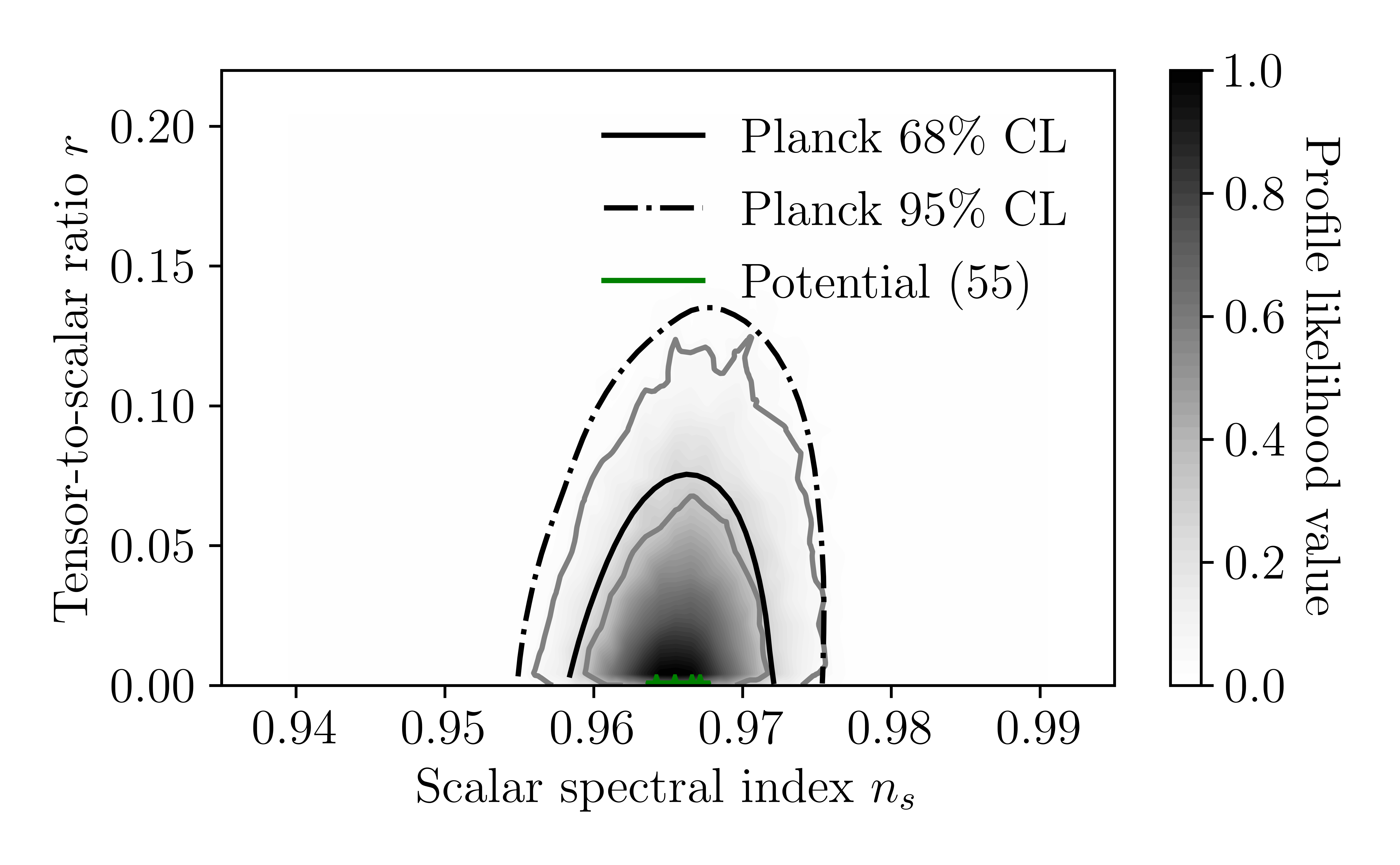
Figure 4: Marginalized curves of the Planck 2018 data and the model with potential $V(\phi)=M\left(1-\frac{d}{\phi}\right)^{2}$ of Eq. (55) vs the Planck 2018 data (green curve) for for $N=[50,65]$ and $(c,d,M,\lambda)=(10^{25.5},-10^{-21},1.48126\times 10^{-24},10^{-16.47})$.

Also the amplitude of the scalar perturbations for the model at hand for $(c,d,M,\lambda)=(10^{25.5},-\frac{1}{10^{21}},2.93436\times 10^{-22}),10^{-17.25}$ is $\mathcal{P}_{\zeta}(k_{*})=2.196\times 10^{-9}$, and actually, the value of the parameter $M$ crucially affects only the amplitude of the scalar perturbations, since all the rest of the inflationary indices are independent of $M$. Now, for $(c,d,M,\lambda)=(10^{25.5},-\frac{1}{10^{21}},2.93436\times 10^{-22}),10^{-17.25}$ the values of the scalar field at the beginning and the end of inflation are $(\phi_{i},\phi_{f})=(8.56165\times 10^{-8},8.38407\times 10^{-16})$, which are sub-Planckian values, thus the model is self-consistent. More importantly, we find that $c_{T}^{2}-1=6.39299\times 10^{-17}$ and also the model well satisfies the constraint (18), since we find that for $(c,d,M,\lambda)=(10^{25.5},-\frac{1}{10^{21}},2.93436\times 10^{-22}),10^{-17.25}$, $c\,\xi H^{2}\sim\mathcal{O}(10^{2})$. Moreover, let us check whether the slow-roll approximations (11) and also the approximations of Eq. (13) hold true. As we found, for $(c,d,M,\lambda)=(10^{25.5},-\frac{1}{10^{21}},2.93436\times 10^{-22}),10^{-17.25}$ we have $\dot{\phi}^{2}\sim\mathcal{O}(10^{-40})$, $c\,\xi\dot{\phi}^{2}\sim\mathcal{O}(10^{-38})$ and $V\sim\mathcal{O}(10^{-22})$, therefore the model is self-consistent and well fitted within the Planck 2018 data.

Let us quote at this point, several other potentials we found that these are viable, without giving many details for brevity. For example, a similar phenomenology with the above potentials is obtained by the potential,

$$V(\phi)=M\left(1-\frac{d}{\phi}\right)^{100}\,.$$ (60)

A rather disturbing feature for this class of models is that the gravitational wave speed is larger than the speed of light, at an acceptable level, but still, it is a mentionable and disturbing feature. Another viable potential of this sort with the scalar coupling function related to the potential as in Eq. (35) is the following,

$$V(\phi)=M\phi^{n}\,,$$ (61)

which however predicts a short inflationary era for viability. For example for $N=30$ $e$-foldings, and for the free parameters chosen as $(c,M,\lambda,n)=(10^{40},-\frac{1}{10^{21}},2.93436\times 10^{-22},10^{16},10^{-15})$, one gets $n_{\mathcal{S}}=0.967638$, $r=1.28053\times 10^{-16}$ and $c_{T}^{2}-1=-5.39374\times 10^{-18}$, thus in this case the gravitational wave speed is smaller than the speed of light, and almost equal to unity. Short viable inflationary eras can be obtained by another class of models, that of Eq. (33). We examined the potential $V(\phi)=V_{0}\phi^{n}$ and we found viability of the model for $N=30$, for various values of the free parameters, but we omit the details for brevity.

III.2 Phenomenology of Unconstrained Models

Now let us consider the unconstrained models which as it proves have less ability to provide viable phenomenologies for a normal duration of the inflationary era. In this case, the first slow-roll index takes the form,

$$\epsilon_{1}=\frac{3V^{\prime}(\phi)^{2}}{2V(\phi)\left(4\sqrt{3}c\xi(\phi)V(\phi)^{3/2}+\sqrt{3}\sqrt{V(\phi)}\right)^{2}}-\frac{3c\xi(\phi)V^{\prime}(\phi)^{2}}{\left(4\sqrt{3}c\xi(\phi)V(\phi)^{3/2}+\sqrt{3}\sqrt{V(\phi)}\right)^{2}}\,,$$ (62)

and the expression entering the $e$-foldings number has the form,

$$\frac{V(\phi)(4c\xi(\phi)V(\phi)+1)}{V^{\prime}(\phi)}\,,$$ (63)

so the functional forms of the kinetic coupling function $\xi(\phi)$ used in the previous section, greatly simplify the above. We shall present one viable model which we found for brevity, using the functional form of $\xi(\phi)$ presented in Eq. (33). We consider the following potential at this point,

$$V(\phi)=\mu\phi^{-n}\,,$$ (64)

and by choosing $\xi(\phi)$ as in Eq. (33) the scalar coupling function $\xi(\phi)$ reads,

$$\xi(\phi)=\lambda\phi^{n}\,,$$ (65)

so the first slow-roll index reads in this case,

$$\epsilon_{1}=\frac{n^{2}(1-2c\lambda\mu)}{2(4c\lambda\mu\phi+\phi)^{2}}\,,$$ (66)

and therefore by solving the equation $|\epsilon_{1}(\phi_{f})|=1$ we get the value of the scalar field at the end of inflationary era $\phi_{f}$ which is,

$$\phi_{f}=\frac{\sqrt{n^{2}-2c\lambda\mu n^{2}}}{\sqrt{2}\sqrt{16c^{2}\lambda^{2}\mu^{2}+8c\lambda\mu+1}}\,,$$ (67)

and by using Eq. (42), the value of the scalar field at first horizon crossing is in this case,

$$\phi_{i}=\frac{\sqrt{-2c\lambda\mu n-4(4c\lambda\mu N+N)+n}}{\sqrt{2}\sqrt{\frac{(4c\lambda\mu+1)^{2}}{n}}}\,.$$ (68)

Now a viable phenomenology is obtained in this case for a short inflationary era with $N=30$ for various values of the free parameters, for example if we choose the free parameters of the model at hand as follows $(c,n,\mu,\lambda)=(10^{30},10^{-15},2.11\times 10^{-25},0.1)$, the spectral index of the scalar perturbations, the tensor-to-scalar ratio and the tensor spectral index take the values $n_{\mathcal{S}}=0.966667$, $r=6.59284\times 10^{-18}$ and $n_{\mathcal{T}}=-8.28735\times 10^{-19}$, hence the model is viable regarding the observational indices of inflation. Also the amplitude of the scalar perturbations for the model at hand for $(c,n,\mu,\lambda)=(10^{30},10^{-15},2.11\times 10^{-25},0.1)$ is $\mathcal{P}_{\zeta}(k_{*})=2.19063\times 10^{-9}$, and actually, the value of the parameter $\mu$ crucially affects only the amplitude of the scalar perturbations. Now, for $(c,n,\mu,\lambda)=(10^{30},10^{-15},2.11\times 10^{-25},0.1)$ the values of the scalar field at the beginning and the end of inflation are $(\phi_{i},\phi_{f})=(2.73863\times 10^{-10},1.76781\times 10^{-19})$, which are in this case too sub-Planckian values, thus the model is self-consistent. More importantly, we find that $c_{T}^{2}-1=2.77781\times 10^{-19}$, in which case we have the disturbing feature of having a gravitational wave speed to be larger than the speed of light, even for a slight extent. Finally, let us check whether the slow-roll approximations (11) and also the approximations of Eq. (13) hold true. As we found, for $(c,n,\mu,\lambda)=(10^{30},10^{-15},2.11\times 10^{-25},0.1)$ we have $\dot{\phi}^{2}\sim\mathcal{O}(10^{-48})$, $c\,\xi\dot{\phi}^{2}\sim\mathcal{O}(10^{-44})$ and $V\sim\mathcal{O}(10^{-25})$, hence the model is self-consistent and also well fitted within the Planck 2018 data.

For completeness, let us mention that many models $\xi(\phi)=\frac{\lambda V^{\prime}(\phi)^{2}}{V(\phi)}$ yield an interesting phenomenology, however all the models have a large tensor-to-scalar ratio, so we will not present these here.

IV Conclusions

In this article we thoroughly studied the inflationary phenomenology of non-minima derivative coupling theories in light of the GW170817 constraints on the speed of gravitational waves. Since spacetime is classical during and after the inflationary era, there is no fundamental reason for the graviton to change its mass, thus the GW170817 constraints even the primordial tensor perturbations, so in this work we formalized the inflationary phenomenology of non-minimal derivative coupling theories, taking also into account the constraints of the GW170817 event. By using the slow-roll assumptions solely, we provided analytic relations for the slow-roll indices and the observational indices of inflation, including the amplitude of scalar perturbations, which are severely constrained by the latest Planck data. We introduced several classes of models, using several convenient relations between the scalar potential $V(\phi)$ and the scalar coupling function $\xi(\phi)$, and we presented in detail their phenomenology. We found several viable models, with interesting features, that are compatible with both the Planck data and the GW170817 event. Some of the viable models predict a tiny deviation of the order $\sim\mathcal{O}(10^{-17}-10^{-19})$ from the speed of light, and actually the propagation speed is slightly larger from that of light, so these models are slightly ghost theories to a very tiny extent. Also some viable models predict a short inflationary period. We presented only some of the possible models that can be used, and as we demonstrated, these theories can be considered as viable candidate theories of inflation, because they also have a theoretical attribute of containing quantum imprints in the inflationary Lagrangian. What we did not seek in this work is whether models exist that may lead to a significantly blue-tilted tensor spectral index, which may have implications for future gravitational wave observations. This task will be the focus of a future work. Also another interesting point is whether the models we presented with a specific scalar Gauss-Bonnet coupling $\xi(\phi)$ are valid only for the inflationary era, or these may be used for other evolutionary eras of our Universe, up to late times. The answer is that these models are valid only for the slow-roll era during the inflationary era, since for reheating and subsequent eras, the Hubble rate is different, so given the potential, the scalar Gauss-Bonnet coupling function $\xi(\phi)$ might be required to be approximated by a distinct function, see the discussion in Ref. [59].

References

- [1] B. P. Abbott et al. [LIGO Scientific and Virgo], Phys. Rev. Lett. 119 (2017) no.16, 161101 doi:10.1103/PhysRevLett.119.161101 [arXiv:1710.05832 [gr-qc]].
- [2] B. P. Abbott et al. [LIGO Scientific, Virgo, Fermi-GBM and INTEGRAL], Astrophys. J. Lett. 848 (2017) no.2, L13 doi:10.3847/2041-8213/aa920c [arXiv:1710.05834 [astro-ph.HE]].
- [3] B. P. Abbott et al. “Multi-messenger Observations of a Binary Neutron Star Merger,” Astrophys. J. 848 (2017) no.2, L12 doi:10.3847/2041-8213/aa91c9 [arXiv:1710.05833 [astro-ph.HE]].
- [4] B. P. Abbott et al. [LIGO Scientific and Virgo], Phys. Rev. D 100 (2019) no.6, 061101 doi:10.1103/PhysRevD.100.061101 [arXiv:1903.02886 [gr-qc]].
- [5] J. M. Ezquiaga and M. Zumalacárregui, Phys. Rev. Lett. 119 (2017) no.25, 251304 doi:10.1103/PhysRevLett.119.251304 [arXiv:1710.05901 [astro-ph.CO]].
- [6] T. Baker, E. Bellini, P. G. Ferreira, M. Lagos, J. Noller and I. Sawicki, Phys. Rev. Lett. 119 (2017) no.25, 251301 doi:10.1103/PhysRevLett.119.251301 [arXiv:1710.06394 [astro-ph.CO]].
- [7] P. Creminelli and F. Vernizzi, Phys. Rev. Lett. 119 (2017) no.25, 251302 doi:10.1103/PhysRevLett.119.251302 [arXiv:1710.05877 [astro-ph.CO]].
- [8] J. Sakstein and B. Jain, Phys. Rev. Lett. 119 (2017) no.25, 251303 doi:10.1103/PhysRevLett.119.251303 [arXiv:1710.05893 [astro-ph.CO]].
- [9] G. Agazie et al. [NANOGrav], Astrophys. J. Lett. 951 (2023) no.1, L8 doi:10.3847/2041-8213/acdac6 [arXiv:2306.16213 [astro-ph.HE]].
- [10] J. Baker, J. Bellovary, P. L. Bender, E. Berti, R. Caldwell, J. Camp, J. W. Conklin, N. Cornish, C. Cutler and R. DeRosa, et al. [arXiv:1907.06482 [astro-ph.IM]].
- [11] T. L. Smith and R. Caldwell, Phys. Rev. D 100 (2019) no.10, 104055 doi:10.1103/PhysRevD.100.104055 [arXiv:1908.00546 [astro-ph.CO]].
- [12] J. Crowder and N. J. Cornish, Phys. Rev. D 72 (2005), 083005 doi:10.1103/PhysRevD.72.083005 [arXiv:gr-qc/0506015 [gr-qc]].
- [13] T. L. Smith and R. Caldwell, Phys. Rev. D 95 (2017) no.4, 044036 doi:10.1103/PhysRevD.95.044036 [arXiv:1609.05901 [gr-qc]].
- [14] N. Seto, S. Kawamura and T. Nakamura, Phys. Rev. Lett. 87 (2001), 221103 doi:10.1103/PhysRevLett.87.221103 [arXiv:astro-ph/0108011 [astro-ph]].
- [15] S. Kawamura, M. Ando, N. Seto, S. Sato, M. Musha, I. Kawano, J. Yokoyama, T. Tanaka, K. Ioka and T. Akutsu, et al. [arXiv:2006.13545 [gr-qc]].
- [16] G. W. Horndeski, Int.J.Theor.Phys. 10, 363 (1974).
- [17] T. Kobayashi, Rept. Prog. Phys. 82 (2019) no.8, 086901 doi:10.1088/1361-6633/ab2429 [arXiv:1901.07183 [gr-qc]].
- [18] T. Kobayashi, Phys. Rev. D 94 (2016) no.4, 043511 doi:10.1103/PhysRevD.94.043511 [arXiv:1606.05831 [hep-th]].
- [19] M. Crisostomi, M. Hull, K. Koyama and G. Tasinato, JCAP 03 (2016), 038 doi:10.1088/1475-7516/2016/03/038 [arXiv:1601.04658 [hep-th]].
- [20] E. Bellini, A. J. Cuesta, R. Jimenez and L. Verde, JCAP 02 (2016), 053 doi:10.1088/1475-7516/2016/06/E01 [arXiv:1509.07816 [astro-ph.CO]].
- [21] J. Gleyzes, D. Langlois, F. Piazza and F. Vernizzi, JCAP 02 (2015), 018 doi:10.1088/1475-7516/2015/02/018 [arXiv:1408.1952 [astro-ph.CO]].
- [22] C. Lin, S. Mukohyama, R. Namba and R. Saitou, JCAP 10 (2014), 071 doi:10.1088/1475-7516/2014/10/071 [arXiv:1408.0670 [hep-th]].
- [23] C. Deffayet and D. A. Steer, Class. Quant. Grav. 30 (2013), 214006 doi:10.1088/0264-9381/30/21/214006 [arXiv:1307.2450 [hep-th]].
- [24] D. Bettoni and S. Liberati, Phys. Rev. D 88 (2013), 084020 doi:10.1103/PhysRevD.88.084020 [arXiv:1306.6724 [gr-qc]].
- [25] K. Koyama, G. Niz and G. Tasinato, Phys. Rev. D 88 (2013), 021502 doi:10.1103/PhysRevD.88.021502 [arXiv:1305.0279 [hep-th]].
- [26] A. A. Starobinsky, S. V. Sushkov and M. S. Volkov, JCAP 06 (2016), 007 doi:10.1088/1475-7516/2016/06/007 [arXiv:1604.06085 [hep-th]].
- [27] S. Capozziello, K. F. Dialektopoulos and S. V. Sushkov, Eur. Phys. J. C 78 (2018) no.6, 447 doi:10.1140/epjc/s10052-018-5939-1 [arXiv:1803.01429 [gr-qc]].
- [28] J. Ben Achour, M. Crisostomi, K. Koyama, D. Langlois, K. Noui and G. Tasinato, JHEP 12 (2016), 100 doi:10.1007/JHEP12(2016)100 [arXiv:1608.08135 [hep-th]].
- [29] A. A. Starobinsky, S. V. Sushkov and M. S. Volkov, Phys. Rev. D 101 (2020) no.6, 064039 doi:10.1103/PhysRevD.101.064039 [arXiv:1912.12320 [hep-th]].
- [30] J. c. Hwang and H. Noh, Phys. Rev. D 71 (2005) 063536 doi:10.1103/PhysRevD.71.063536 [gr-qc/0412126].
- [31] S. Capozziello, G. Lambiase and H. J. Schmidt, Annalen Phys. 9 (2000), 39-48 doi:10.1002/(SICI)1521-3889(200001)9:139::AID-ANDP393.0.CO [arXiv:gr-qc/9906051 [gr-qc]].
- [32] S. Capozziello and G. Lambiase, Gen. Rel. Grav. 31 (1999), 1005-1014 doi:10.1023/A:1026631531309 [arXiv:gr-qc/9901051 [gr-qc]].
- [33] S. V. Sushkov, Phys. Rev. D 80 (2009), 103505 doi:10.1103/PhysRevD.80.103505 [arXiv:0910.0980 [gr-qc]].
- [34] M. Minamitsuji, Phys. Rev. D 89 (2014), 064017 doi:10.1103/PhysRevD.89.064017 [arXiv:1312.3759 [gr-qc]].
- [35] E. N. Saridakis and S. V. Sushkov, Phys. Rev. D 81 (2010), 083510 doi:10.1103/PhysRevD.81.083510 [arXiv:1002.3478 [gr-qc]].
- [36] A. Barreira, B. Li, A. Sanchez, C. M. Baugh and S. Pascoli, Phys. Rev. D 87 (2013), 103511 doi:10.1103/PhysRevD.87.103511 [arXiv:1302.6241 [astro-ph.CO]].
- [37] S. Sushkov, Phys. Rev. D 85 (2012), 123520 doi:10.1103/PhysRevD.85.123520 [arXiv:1204.6372 [gr-qc]].
- [38] A. Barreira, B. Li, C. M. Baugh and S. Pascoli, Phys. Rev. D 86 (2012), 124016 doi:10.1103/PhysRevD.86.124016 [arXiv:1208.0600 [astro-ph.CO]].
- [39] M. A. Skugoreva, S. V. Sushkov and A. V. Toporensky, Phys. Rev. D 88 (2013), 083539 doi:10.1103/PhysRevD.88.083539 [arXiv:1306.5090 [gr-qc]].
- [40] G. Gubitosi and E. V. Linder, Phys. Lett. B 703 (2011), 113-118 doi:10.1016/j.physletb.2011.07.066 [arXiv:1106.2815 [astro-ph.CO]].
- [41] J. Matsumoto and S. V. Sushkov, JCAP 11 (2015), 047 doi:10.1088/1475-7516/2015/11/047 [arXiv:1510.03264 [gr-qc]].
- [42] C. Deffayet, O. Pujolas, I. Sawicki and A. Vikman, JCAP 10 (2010), 026 doi:10.1088/1475-7516/2010/10/026 [arXiv:1008.0048 [hep-th]].
- [43] L. Granda and W. Cardona, JCAP 07 (2010), 021 doi:10.1088/1475-7516/2010/07/021 [arXiv:1005.2716 [hep-th]].
- [44] J. Matsumoto and S. V. Sushkov, JCAP 01 (2018), 040 doi:10.1088/1475-7516/2018/01/040 [arXiv:1703.04966 [gr-qc]].
- [45] C. Gao, JCAP 06 (2010), 023 doi:10.1088/1475-7516/2010/06/023 [arXiv:1002.4035 [gr-qc]].
- [46] L. Granda, JCAP 07 (2010), 006 doi:10.1088/1475-7516/2010/07/006 [arXiv:0911.3702 [hep-th]].
- [47] C. Germani and A. Kehagias, Phys. Rev. Lett. 105 (2010), 011302 doi:10.1103/PhysRevLett.105.011302 [arXiv:1003.2635 [hep-ph]].
- [48] C. Fu, P. Wu and H. Yu, Phys. Rev. D 100 (2019) no.6, 063532 doi:10.1103/PhysRevD.100.063532 [arXiv:1907.05042 [astro-ph.CO]].
- [49] M. Petronikolou, S. Basilakos and E. N. Saridakis, Phys. Rev. D 106 (2022) no.12, 124051 doi:10.1103/PhysRevD.106.124051 [arXiv:2110.01338 [gr-qc]].
- [50] S. Karydas, E. Papantonopoulos and E. N. Saridakis, Phys. Rev. D 104 (2021) no.2, 023530 doi:10.1103/PhysRevD.104.023530 [arXiv:2102.08450 [gr-qc]].
- [51] A. Dima and F. Vernizzi, Phys. Rev. D 97 (2018) no.10, 101302 doi:10.1103/PhysRevD.97.101302 [arXiv:1712.04731 [gr-qc]].
- [52] C. D. Kreisch and E. Komatsu, JCAP 12 (2018), 030 doi:10.1088/1475-7516/2018/12/030 [arXiv:1712.02710 [astro-ph.CO]].
- [53] S. Arai and A. Nishizawa, Phys. Rev. D 97 (2018) no.10, 104038 doi:10.1103/PhysRevD.97.104038 [arXiv:1711.03776 [gr-qc]].
- [54] C. Cartier, J. c. Hwang and E. J. Copeland, Phys. Rev. D 64 (2001), 103504 doi:10.1103/PhysRevD.64.103504 [arXiv:astro-ph/0106197 [astro-ph]].
- [55] Y. Akrami et al. [Planck], Astron. Astrophys. 641 (2020), A10 doi:10.1051/0004-6361/201833887 [arXiv:1807.06211 [astro-ph.CO]].
- [56] V. K. Oikonomou, Class. Quant. Grav. 38 (2021) no.19, 195025 doi:10.1088/1361-6382/ac2168 [arXiv:2108.10460 [gr-qc]].
- [57] V. K. Oikonomou and F. P. Fronimos, Class. Quant. Grav. 38 (2021) no.3, 035013 doi:10.1088/1361-6382/abce47 [arXiv:2006.05512 [gr-qc]].
- [58] S. D. Odintsov, V. K. Oikonomou and F. P. Fronimos, Nucl. Phys. B 958 (2020), 115135 doi:10.1016/j.nuclphysb.2020.115135 [arXiv:2003.13724 [gr-qc]].
- [59] V. K. Oikonomou, P. Tsyba and O. Razina, Annals Phys. 462 (2024), 169597 doi:10.1016/j.aop.2024.169597 [arXiv:2401.11273 [gr-qc]].