A Study of the Generalized Naming Game and Bayesian Naming Game as Dynamical Systems

Abstract

We study the $\beta$-model ($\beta$-NG) and the Bayesian Naming Game (BNG) as dynamical systems. By applying linear stability analysis to the dynamical system associated with the $\beta$-model, we demonstrate the existence of a non-generic bifurcation with a bifurcation point $\beta_{c}=1/3$. As $\beta$ passes through $\beta_{c}$, the stability of isolated fixed points changes, giving rise to a one-dimensional manifold of fixed points. Notably, this attracting invariant manifold forms an arc of an ellipse. In the context of the BNG, we propose modeling the Bayesian learning probabilities $p_{A}$ and $p_{B}$ as logistic functions. This modelling approach allows us to establish the existence of fixed points without relying on the overly strong assumption that $p_{A}=p_{B}=p$, where $p$ is a constant.

I Introduction

The naming game is a multi-agent model that aims to simulate the spontaneous emergence of consensus among agents who interact pairwise according to two possible processes: agreement and word/name learning Baronchelli et al. [2006]; Blythe [2015]; Baronchelli [2016]; Chen and Lou [2019]; Marchetti et al. [2020a]. In its simplest realization, the agents are allowed to learn only two possible names, denoted here by the symbols A and B, according to some basic rules (we refer the reader to Refs. Baronchelli [2016]; Marchetti et al. [2020a] for their definitions). Furthermore, if the underlying topology on which the agents may lie, is neglected altogether Castello et al. [2009]; Marchetti et al. [2020a], we refer to such a model as the minimal naming game (MNG).

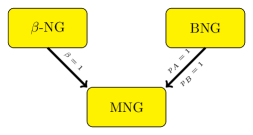
Figure 1: The cartoon depicts the relationship between the MNG, $\beta$-NG, and BNG through their characteristic parameters: $\beta\in[0,1]$ and the learning probabilities $p_{A},p_{B}\in[0,1]$. Setting $\beta$ and $p_{A},p_{B}$ to unity in $\beta$-NG and BNG models, respectively, one recovers the MNG.

The MNG model can be thought as a particular case of two variants: the generalized naming game ($\beta$-NG) Baronchelli et al. [2007] and the Bayesian naming game (BNG) Marchetti et al. [2020b, a, 2021]. Both variants add human features otherwise absent in agents of MNG. In $\beta$-NG, a parameter $\beta$ is introduced to take into account the probability of acknowledged influence Friedkin [1990], thus affecting the agreement processes, while in BNG the name learning processes are now dictated by the time-dependent probabilities $p_{A}\equiv p_{A}\left(t\right)$ and $p_{B}\equiv p_{B}\left(t\right)$ necessary for generalizing the concept $\mathcal{C}$ associated with words A and B, respectively  Tenenbaum [1999]; Tenenbaum and Griffiths [2001]; Murphy [2012]. It is worth noting here that such probabilities are a direct consequence of Bayes rule Jeffreys [1939]. Therefore, according to the latter model the agents become Bayesian-rational individuals that in an uncertain world find their best action using the laws of probability de Finetti [1989]; Aumann [1976]; Aaronson [2005]; Sanborn and Chater [2016]. That being said, the minimal naming game can be recovered from the above two variants by setting their characteristic parameters, i.e. $\beta$ and $p_{A},p_{B}$, to unity as illustrated in cartoon of Fig. 1.

The dynamics of the naming game is routinely investigated through computer simulations of multi-agent systems. The simulations allow for the computation of the observables of interest, e.g. the convergence time, the success rate, averaging over several hundred realizations Marchetti et al. [2020a]. However, the differential equations dictating the time-evolution for each model, can be also derived, assuming the mean-field approximation, thus offering an alternative approach to study some features of consensus dynamics. In fact, the differential equations of these models form two-dimensional (2D) dynamical systems whose study has some evident advantages. First, due to their low dimensionality, the time-evolution is much simpler when compared to that of naming game models where multiple names need to be taken into account Ma et al. [2023]. Second, one can exploit the methods provided by the dynamical systems theory Strogatz [2018]; Hirsch et al. [2013], such as bifurcation diagrams and phase portraits for autonomous systems, to infer whether or not the consensus emerges without the need to perform the numerical simulations, a task that becomes computationally expensive when the system size $N$, i.e., the number of agents, increases.

In this paper, we shall pursue the latter approach, thereby finding novel interesting dynamical features that, to our best knowledge, have been overlooked so far.

In Section II the linear stability (LSA) applied systematically to $\beta$-NG shows that such a dynamical system undergoes to a non-generic bifurcation with bifurcation point $\beta=\beta_{c}$ ($\beta_{c}=1/3$), where several things happen simultaneously. The isolated fixed points $A=\left(1,0\right)$, $B=\left(0,1\right)$ and $C=\left(c_{\beta},c_{\beta}\right)$ whose coordinates in terms of parameter $\beta$ are given by $c_{\beta}=\left(5\beta+1-\sqrt{\Delta}\right)/4\beta$ where $\Delta\equiv 1+10\beta+9\beta^{2}$ , change their stability and join an emerging one-dimensional manifold of fixed points when $\beta$ goes through $\beta_{c}$. Such an attracting invariant manifold is shown to be an arc of an ellipse (see Figs. 4, 5). This is analog of the non-generic bifurcation observed in 1D differential equation $\dot{z}=\xi\left(z-z^{3}\right)$ at $\xi=0$ ($\xi$ is a parameter) with fixed isolated points $0,\pm 1$. In fact, as $\xi$ passes through $0$, the fixed points at $z=0$, $z=1$, and $z=–1$ change stability and a line of fixed points emerges (the whole $z$-axis is filled with fixed points when $\xi=0$). This is a very degenerate situation because the single parameter $\xi$ affects both the linear and the cubic term in the differential equation simultaneously, causing both terms to vanish when $\xi=0$. Note that the flow of the above 1D differential equation is similar to the 2D flow along the attracting invariant manifold corresponding to the (orange) stable “line” in the bifurcation diagram (see Fig. 2) and to the (orange) curve in the 2D phase plane (see Fig. 4).

We conclude Section II by briefly mentioning the connection between this non-generic bifurcation and the type of noise characterizing the trajectories obtained from the multi-agent simulations, which are now viewed as stochastic processes Erban et al. [2009]; Oksendal [2010].

In Section III, we shall address the issue related to the lack of spontaneous symmetry breaking for the dynamical system associated with BNG. This issue arises when attempting to find the solution by numerically integrating the respective first-order differential system, assuming the initial condition $I_{0}=\left(0.5,0.5\right)$ and setting $p_{A}=p_{B}=p$ where $p$ is a constant, simultaneously.

Denoting the solution as $\left(x,y\right)$, where $x\equiv x\left(t\right)$ and $y\equiv y\left(t\right)$ are the population fractions having either A or B in their inventories at time $t$ respectively, it is found that $\left(x,y\right)$ asymptotically converges to $\left(0.38,0.38\right)$. Thus, there is no convergence to consensus, similar to what occurs with MNG for the very same initial setup Castellano et al. [2009]; Marchetti et al. [2020a].

This is in contrast to what is found in multi-agent simulations, where consensus always emerges either at A or at B for MNG and BNG models. It has already been noted that such a discrepancy between simulations and dynamical systems arises from the fact that the dynamical system approach cannot account for the ubiquitous density fluctuations, or equivalently noise, present in numerical simulations Castellano et al. [2009]. However, this issue is particularly significant here, as the above setup was used to prove the existence of consensus for the dynamical system associated with BNG Marchetti et al. [2020b].

To address this serious problem, we propose modeling the Bayesian probabilities as time-dependent logistic functions (see Eq. 12) James et al. [2023]. Subsequently, by numerically integrating the modified equations, we demonstrate that consensus consistently emerges at either A or B. This outcome is attributed to the spontaneous symmetry breaking induced by the time-dependent probabilities, disrupting the invariance under the swap of variables $x$ and $y$ (see Eqs. 10 and  11). Accordingly, the solution closely resembles that obtained from multi-agent simulations with system size $N\gtrsim 200$ Marchetti et al. [2020b].

II The $\beta$-NG model as Dynamical System

In mean-field approximation the time-evolution of $\beta$-NG model is dictated by the following system of first-order differential equations:

$$\dot{x}=-xy+\beta\left(1-x-y\right)^{2}+Kx\left(1-x-y\right)\,,$$ (1)

$$\dot{y}=-xy+\beta\left(1-x-y\right)^{2}+Ky\left(1-x-y\right)\,,$$ (2)

where $\dot{x},\dot{y}$ the derivatives of $x,y$, with respect to time. We set $K\equiv\left(3\beta-1\right)/2$ in Eqs. 1, 2 while $\beta\in[0,1]$. Next, setting $\dot{x}=0$ and $\dot{y}=0$ into Eqs.1 and 2, it was previously determined that three isolated fixed points exist: A, B, and CBaronchelli et al. [2007]; Castellano et al. [2009]. Applying the LST revealed a first-order non-equilibrium transition at $\beta=\beta_{c}$. Furthermore, the system converges to point C for $\beta<\beta_{c}$, leaving a fraction of undecided agents equal to $1-2c_{\beta}$, while a spontaneous emergence of consensus occurs at either A or B for $\beta>\beta_{c}$. These findings are summarized in the first and third columns of Table 1.

While the above analysis is certainly correct and has been confirmed by multi-agent simulations, it does not address the non-generic bifurcation that characterizes the dynamical system in question.

In the following, we shall unravel the dynamical features of the dynamical system by applying the LSA to the problem at hand in a systematic way. First, let us define the functions $f_{1}\left(x,y\right),f_{2}\left(x,y\right)$ such that $\dot{x}=f_{1}\left(x,y\right),\dot{y}=f_{2}\left(x,y\right)$ according to Eqs. 1, 2. It is then possible to compute the eigenvalues of the following Jacobian matrix $J$ evaluated at a given fixed equilibrium point with Cartesian coordinates $\left(\tilde{x},\tilde{y}\right)$ Strogatz [2018]

$$J=\begin{pmatrix}\partial_{x}f_{1}\left(\tilde{x},\tilde{y}\right)&\partial_{y}f_{1}\left(\tilde{x},\tilde{y}\right)\\ \partial_{x}f_{2}\left(\tilde{x},\tilde{y}\right)&\partial_{y}f_{2}\left(\tilde{x},\tilde{y}\right)\end{pmatrix}\,,$$ (3)

where the symbols $\partial_{x}$, $\partial_{y}$ denote the partial derivatives of $f_{1}\left(x,y\right)$, $f_{2}\left(x,y\right)$ with respect to $x,y$, respectively.

Second, the local equilibrium character of each fixed point can be determined by the eigenvalues of the corresponding matrix $J$. In particular, their equilibrium character is easily identified by looking at the inequalities between the eigenvalues as shown in the trace-determinant plane (also called the bifurcation diagram) (see Fig. 2)  Hirsch et al. [2013]; Perez-Garcia et al. [2019]).

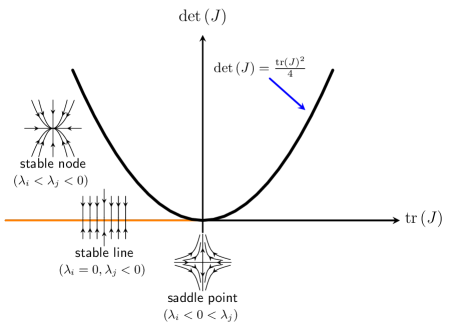
Figure 2: The types of the equilibria for the dynamical system with Eqs. 1, 2 and $\beta\in[0,1]$ according to LSA, in the trace-determinant plane. The respective inequalities between the two (real) eigenvalues $\lambda_{i},\lambda_{j}$ ($i\neq j$) of the matrix $J$ evaluated at each type of fixed point are also shown. The parabola in the (black) solid line corresponds to $\operatorname{tr}\left(J\right)^{2}-4\det\left(J\right)=0$. Note that all the saddle points lie on quadrants III and IV of the trace-determinant plane.

The matrix $J$’s entries evaluated at the fixed point A read: $J_{11}=-K$, $J_{12}=-1-K$, $J_{21}=0$, $J_{22}=-1$ while the matrix entries takes the values $J_{11}=-1$, $J_{12}=0$, $J_{21}=-1-K$, $J_{22}=-K$ when computed at B. Since in both cases the traces and the determinants of the Jacobian matrices are the same, i.e. $\operatorname{tr}\left(J\right)=-1-K$ and $\det\left(J\right)=K$, one must conclude that these matrices have same eigenvalues. Therefore, the fixed points $A,B$ present the very same stability behaviour for each value of $\beta$ in $[0,1]$. Accordingly, in the following we shall focus on the equilibrium character of A only, denoting its corresponding eigenvalues by the symbols $\lambda_{1},\lambda_{2}$. By means of the equations $\operatorname{tr}\left(J\right)=\lambda_{1}+\lambda_{2}$ and $\det\left(J\right)=\lambda_{1}\lambda_{2}$, one immediately finds these two real eigenvalues: $\lambda_{1}=-1$ and $\lambda_{2}=-K$. Since $\lambda_{1}$ is always negative, both eigenvalues are negative when $\beta>\beta_{c}$, while $\lambda_{2}>0$ when $\beta<\beta_{c}$ (see Fig. 3). Looking at the classification scheme in Fig. 2, one must conclude that $A,B$ are saddle points and asymptotically stable nodes for $\beta\in[0,\beta_{c})$ and $\beta\in(\beta_{c},1]$, respectively. So far, the results agree with those reported in Ref. Baronchelli et al. [2007]. However, at $\beta=\beta_{c}$, $\lambda_{2}=0$, and hence both A and B must belong to the stable line corresponding to the negative half-axis (see the (orange) solid line in Fig. 2). Therefore, A and B cannot be longer considered isolated, but according to LSA there must exist an infinite number of other fixed points. We will return to this point later.

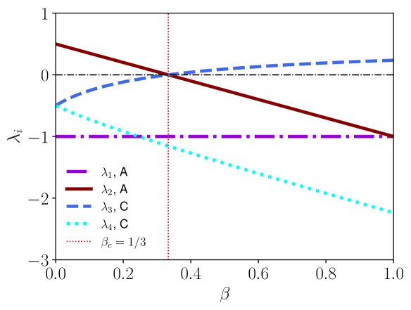
Figure 3: The real eigenvalues $\lambda_{i}$ with $i=1,2$ and $i=3,4$ corresponding to the Jacobian matrix J (Eq. 9) evaluated at A and $C$, respectively, as functions of the parameter $\beta$. The vertical (dotted) line corresponds to $\beta=\beta_{c}$.

We now turn our attention to the equilibrium character of the fixed point $C$, denoting its corresponding eigenvalues by $\lambda_{3}$ and $\lambda_{4}$. To this end, we shall compute them by means of the following formula  Sagués and Epstein [2003]

$$\lambda_{3},\lambda_{4}=\frac{1}{2}\left(\operatorname{tr}\left(J\right)\pm\sqrt{\operatorname{tr}\left(J\right)^{2}-4\det\left(J\right)}\right)\,.$$ (4)

In Fig. 3 we plot $\lambda_{3},\lambda_{4}$ as function of $\beta$ by means of Eq.. 4. From a direct comparison of the corresponding curves with those of $\lambda_{1},\lambda_{2}$, one immediately concludes that $C$ has the opposite equilibrium character of A and B for each each $\beta\in[0,1]\setminus\{\beta_{c}\}$, see Fig. 3. However, when $\beta=\beta_{c}$, $C$ belongs to the stable line as well because $\lambda_{3}=0$ while $\lambda_{4}$ negative (see Fig. 2).

Noting that the stable line is characterized by $\operatorname{tr}\left(J\right)<0$ and $\det\left(J\right)=0$, the last important result could also be obtained without the need to compute the eigenvalues, as follows. First, we note that at $C=\left(c_{\beta},c_{\beta}\right)$, the matrix $J$’s entries must satisfy the identities $J_{11}=J_{22}$ and $J_{12}=J_{21}$, thus the Jacobian matrix is now symmetric. Second, $J_{11},J_{12}$ take the following form as functions of $\beta$

$$J_{11}=-\left(\frac{\beta+1}{2}\right)+\left(\frac{1-\beta}{2}\right)c_{\rm\beta}\,,$$ (5)

and

$$J_{12}=-2\beta+\left(\frac{5\beta-1}{2}\right)c_{\rm\beta}\,,$$ (6)

respectively.

Therefore, in such a case $\operatorname{tr}\left(J\right)=2J_{11}$ and $\det\left(J\right)=J_{11}^{2}-J_{12}^{2}$. Now noting that $\det\left(J\right)=\left(J_{11}+J_{12}\right)\left(J_{11}-J_{12}\right)$, one finds that

$$J_{11}-J_{12}=K\left(1-2c_{\beta}\right)\,.$$ (7)

So, as $K=0$ when $\beta=\beta_{c}$, it follows that the left hand side of Eq. 7, and hence $\det\left(J\right)$ are both zero. Next, we note that the corresponding trace is negative, i.e. $\operatorname{tr}\left(J\right)=2/3\left(c_{\beta}-2\right)<0$, because $c_{\beta}=2-\sqrt{3}\approx 0.26$.

Overall, our analysis shows that the fixed points $A,B,C$ exist for all values of the parameter $\beta$ but there an exchange of stabilities between $A,B$ and $C$ as $\beta$ passes through $\beta_{c}$. In this regard, we can say that the dynamical system undergoes a non-generic bifurcation similar to that of the 1D differential equation discussed in Section I. For the sake of completeness, we summarize all these findings in Table 1.

Table 1: The classification of the fixed points $A,B,C$ according to the linear stability theory. Note that when the isolated equilibrium points are stable, they are also asymptotically stable. The fixed points $A,B,C$ are no longer isolated at bifurcation point $\beta=\beta_{c}$.

Fixed Point	$\beta\in[0,\beta_{c})$	$\beta=\beta_{c}$	$\beta\in(\beta_{c},1]$
A	saddle point	stable line	stable node
B	saddle point	stable line	stable node
C	stable node	stable line	saddle point

Next, the existence of a continuum of fixed points at the bifurcation point could be easily inferred by examining the streamline plot of the velocity field $\mathbf{v}=\left(\dot{x},\dot{y}\right)$ corresponding to Eqs. 1, 2. To this end, in Fig. 4 we plot such a velocity field on the model’s domain in Cartesian $xy$-plane: $\{(x,y)\in\mathbb{R}^{2}:0\leq x\leq 1,0\leq y\leq 1,0\leq x+y\leq 1\}$. It is then evident that there exists one-dimensional manifold of fixed points (orange solid line), and that all trajectories approach it along parallel lines. This finding is consistent with the stable line, that is, the negative negative half-axis of trace $\operatorname{tr}J$, obtained from LSA (see Fig. 2).

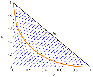
Figure 4: Streamline plot of $\mathbf{v}=\left(\dot{x},\dot{y}\right)$ corresponding to Eqs. 1, 2 at bifurcation point $\beta=\beta_{c}$. Here the curve (orange) of the attracting invariant manifold corresponds to the graph of the map $x\mapsto 1/2\left(-\sqrt{3}\sqrt{4x-x^{2}}+x+2\right)$ with $x\in[0,1]$. The important initial condition $I_{0}=\left(0.5,0.5\right)$ is also shown.

We now prove that the above one-dimensional manifold constitutes an arc of an ellipse. First, its Cartesian equation can be obtained by setting $\beta=\beta_{c}$ and either $\dot{x}=0$ or $\dot{y}=0$ into Eqs. 1, 2. One then finds that the set of points must satisfy the following second-order degree polynomial equation in the variables $x,y$

$$x^{2}-xy+y^{2}-2x-2y+1=0\,.$$ (8)

According to Eq. 8 the one-dimensional manifold corresponds to the graph of the function $x\mapsto 1/2\left(-\sqrt{3}\sqrt{4x-x^{2}}+x+2\right)$ with $x\in[0,1]$. Next, we construct the symmetric matrix $M$ of the quadratic form associated with Eq. 8 in order to classify it as a nondegenerate conic section Apostol [1969]. In the present case, one finds

$$M=\begin{pmatrix}1&0.5\\ 0.5&1\end{pmatrix}\,,$$ (9)

with determinant $\det\left(M\right)=3/4$. As a consequence its eigenvalues must have the same sign, so Eq. 8 yield a conic section that is an ellipse with semi-major axis, semi-minor axis and eccentricity corresponding to $a=\sqrt{6}$, $b=\sqrt{2}$ and $e=\sqrt{2/3}$, respectively. The graph of such an ellipse with its center $0=\left(2,2\right)$ and foci $F_{1}=\left(2-\sqrt{2},2-\sqrt{2}\right)$ and $F_{2}=\left(2+\sqrt{2},2+\sqrt{2}\right)$ is shown in Fig. 5. Note that in such a case, point $C$ now has coordinates $\left(c_{\beta_{c}},c_{\beta_{c}}\right)$ with $c_{\beta_{c}}=2-\sqrt{3}$ and hence lies on the ellipse between points A and B.

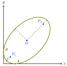
Figure 5: The graph of the ellipse with Eq. 8 emerging at bifurcation point $\beta=\beta_{c}$. The ellipse’s center and foci are $0=\left(2,2\right)$, $F_{1}=\left(2-\sqrt{2},2-\sqrt{2}\right)$ and $F_{2}=\left(2+\sqrt{2},2+\sqrt{2}\right)$, respectively. The fixed points $A=\left(1,0\right)$, $B=\left(0,1\right)$ and $C=\left(c_{\beta_{c}},c_{\beta_{c}}\right)$ where $c_{\beta_{c}}=2-\sqrt{3}$ are no longer isolated equilibria.

We conclude this section by noting another important consequence of the existence of a non-generic bifurcation. The dynamical system approach provides a deterministic mean-field description of the $\beta$-model, but the trajectories from its multi-agent simulations are intrinsically noisy. Therefore, one would expect that there is some effect of noise close to the bifurcation Erban et al. [2009].

To illustrate this, let us consider $x$, or equivalently $y$, obtained from a single run of a simulation starting from $I_{0}$ as a random variable $X_{t}$. In Fig. 6, we plot six randomly chosen sample paths of $X_{t}$ as functions of time from simulations with $N=1,000$ agents. Note that the paths labeled by $\omega=1,2,3$ and $\omega=4,5,6$ correspond to $\beta=0.2$ and $\beta=\beta_{c}$, respectively where each $\omega_{i}$ could be understood as a specific outcome in the sample space.

The paths with $\omega=1,2,3$ exhibit a pattern completely different from those at the bifurcation point, i.e., with $\omega=4,5,6$. While the former remain close to the sample mean $E[X_{t}]$ (black solid line) computed from $1,200$ trajectories, thus showing the typical mean-returning behavior of the Ornstein-Uhlenbeck (OU) process Uhlenbeck and Ornstein [1930]; Vasicek [1977], the latter seem to wander in a more random fashion. Preliminary statistical analysis Marchetti [prep] confirms that the sample paths at $\beta=0.2$ belong to OU process, while those at bifurcation point to a nonstandard Brownian motion Einstein [1905]; Langevin [1908]; Wiener [1923]; Ritort [2019].

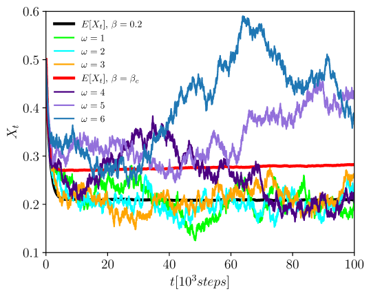
Figure 6: Randomly chosen sample paths of $X_{t}$ ($X_{0}=0.5$) as functions of time $t$ from multi-agents simulations with $N=1,000$ agents. The paths with label $\omega=1,2,3$ and $\omega=4,5,6$ correspond to $\beta=0.2$ and $\beta=\beta_{c}$, respectively. Solid lines in black color and red color correspond to sample mean $E[X_{t}]$ computed from $1,200$ trajectories for $\beta=0.2$ and $\beta=\beta_{c}$, respectively.

III The Bayesian Naming Game as a Dynamical System

According to the BNG model, agents must learn new, unknown names through their previous experiences and background knowledge. Furthermore, since the learning process occurs under uncertainty, a probabilistic approach is necessary for modeling such a process. In this context, a Bayesian framework proposed by Tenenbaum and co-workers seems appropriate Tenenbaum [1999]; Murphy [2012]; Griffiths and Tenenbaum [2006]; Griffiths and Kalish [2007]; Tenenbaum et al. [2011]; Perfors et al. [2011]; Lake et al. [2015]. As a result of this probabilistic framework, agents attempt to generalize the concept $\mathcal{C}$ associated with the names A and B by computing the learning probabilities $p_{A}$ and $p_{B}$, respectively. These probabilities depend on the positive examples stored by the agents during their pairwise interactions. In this regard, the BNG model paves the way for incorporating many human cognitive biases Tversky and Kahneman [1974]; Kahneman [2012]; Hahn [2014]; Sanborn and Chater [2016]; Ngampruetikorn and Stephens [2016]; Madsen et al. [2018] into the consensus dynamics, which were out of reach for the previous variants of naming game.

Assuming the mean-field approximation, the time evolution of BNG is governed by the following non-autonomous first-order differential system Marchetti et al. [2020b]:

$$\dot{x}=-p_{B}xy+\left(1-x-y\right)^{2}+\frac{3-p_{B}}{2}x\left(1-x-y\right)\,,$$ (10)

$$\dot{y}=-p_{A}xy+\left(1-x-y\right)^{2}+\frac{3-p_{A}}{2}y\left(1-x-y\right)\,.$$ (11)

Note that finding a solution to the above system is not possible without making some reasonable assumptions about the probabilities $p_{A}\left(t\right)$ and $p_{B}\left(t\right)$, both falling within the interval [0,1] with an unknown functional form. In Ref.Marchetti et al. [2020b], it was proposed to set $p_{A}=p_{B}=p$, thus making the probabilities identical and time-independent at the same time. While this assumption, along with the initial condition $I_{0}$, played a crucial role in estimating an upper bound of about $20\%$ for the number of agents with two names in their inventories Marchetti et al. [2021] , it cannot be used to demonstrate the existence of fixed points A and B in full generality, as wrongly assumed in Ref.  Marchetti et al. [2020b]. In fact, consensus cannot be reached in such an initial setup due to the absence of spontaneous symmetry breaking Goldstone [1961]; Michel [1980] , similar to what happens to the dynamical system associate with MNG (see Section I).

Next, we shall demonstrate that the assumption $p_{A}=p_{B}=p$ cannot be valid throughout the entire time-evolution of the dynamical system associated with BNG. To illustrate this fact we computed cumulative distribution function (CDF) of the values taken by $p_{A}$ and $p_{B}$ during a single run of a system with size $N=3,000$ with initial condition corresponding to $50\%$ of the agents knowing the word A and the remainder knowing the other word B Marchetti et al. [2020b] . The simulation data were obtained assuming the Erlang prior and different thresholds $n^{\ast}_{ex,A}=5$, and $n^{\ast}_{ex,B}=6$, of the number of positive examples stored by the agents, necessary for computing the probabilities $p_{A}$ and $p_{B}$, respectively. As a consequence of the last assumption, the words A and B are now distinguishable synonyms, and, at the same time, the learning of A is favored Marchetti et al. [2020b].

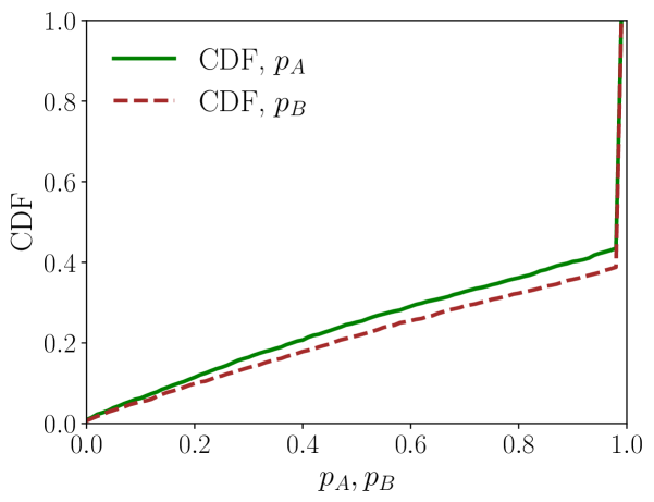
Figure 7: The cumulative distribution function of $p_{A}$ (solid line) and $p_{B}$ (dashed line) as a function of the Bayesian probabilities $p_{A}$ and $p_{B}$, respectively, obtained from a simulation of a system with size $N=3,000$, starting from the initial condition $I_{0}$, and assuming the Erlang prior. The name learning thresholds for A and B, were $n^{\ast}_{ex,A}=5$ and $n^{\ast}_{ex,B}=6$, respectively. In such a case the consensus is reached at A.

In Fig. 7, the curves corresponding to CDF of $p_{A}$ (solid line) and $p_{B}$ (dashed line) are shown as functions of the Bayesian probabilities. From their different trends, it is clear that the assumption $p_{A}=p_{B}=p$ is untenable and may only be valid for a short time-interval. Furthermore, there is also a step-like progression toward unity in the two cumulative distribution functions as a direct consequence of the few-shot learning processes Tenenbaum [1999]. The latter feature of this model demonstrates that it is implausible to consider such probabilities as smooth functions either of the number of positive examples or of time. Regarding their time-dependence, we cannot infer its exact functional form directly from the multi-agent simulations, due to their strong dependence on the system size $N$. However, Bayesian probabilities exhibit an evident monotonically increasing trend with time within a mean-field approximation Marchetti et al. [2020b].

With the above considerations in mind, we propose modeling both $p_{A}\left(t\right)$ and $p_{B}\left(t\right)$ as a time-dependent logistic function (or sigmoid function) Murphy [2012] . The logistic function has a S-shaped form that can be modified appropriately thanks to its two characteristic parameters: the logistic growth rate (or the steepness of the curve) $\eta$, and the quantity $t_{m}$ that corresponds to the value of $t$ of function’s midpoint. Denoting it by the symbol $g$, the logistic function reads:

$$g\left(t\right)=\frac{1}{1+\exp\left(-\eta\left(t-t_{m}\right)\right)}\,.$$ (12)

In the following, we shall give an example of how our probabilistic modeling yields reasonable results in accordance with the numerical simulations. Without the loss of generality, we chose the following three values for parameters $\eta$ and $t_{m}$: $\eta=2$, $t_{m,A}=10$ and $t_{m,B}=130$. Inserting $\eta=2,t_{m,A}=10$ and $\eta=2,t_{m,B}=130$ into Eq. 12 we get two different logistic functions: $g_{A}$ and $g_{B}$, respectively. While such a value of $\eta$ guarantees that both $g_{A}$ and $g_{B}$ are step-like non-smooth functions of time $t$, the different values of $t_{m}$ i.e. $t_{m,A}$, $t_{m,B}$, differentiate $g_{A}$ from $g_{B}$. Furthermore, our choice of parameters ensures that the learning of name A will be favored. In the inset of Fig. 8, the logistic functions $g_{A}$ (solid line) and $g_{B}$ (dashed line) are shown as functions of time $t$.

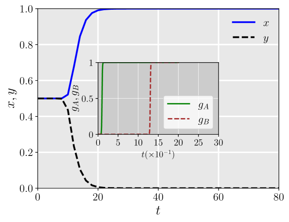
Figure 8: Numerical solution of Eqs. 10, 11 replacing the probabilities $p_{A}$ and $p_{B}$ with the logistic functions $g_{A}$ and $g_{B}$, respectively. The logistic function’s parameters used are $\eta=2$ for both $g_{A}$ and $g_{B}$, $t_{m,A}=10$ and $t_{m,B}=130$ for $g_{A}$ and $g_{B}$, respectively. The initial condition is $I_{0}=\left(0.5,0.5\right)$. (Inset) The logistic functions $g_{A}$ (solid line) and $g_{B}$ (dashed line) under scrutiny as functions of time $t$.

Next, we proceed to numerically integrate Eqs. 10, 11, replacing $p_{A}$ with $g_{A}$ and $p_{B}$ with $g_{B}$, using the algorithm LSODA Petzold [1983], and assuming the initial condition $I_{0}=\left(0.5,0.5\right)$. The numerical result shows that the solution $\left(x,y\right)$ asymptotically converges to $A=\left(1,0\right)$ (see Fig. 8). Accordingly, there exists now a spontaneous emergence of consensus despite the dynamics following a mean-field deterministic prescription. Furthermore, by swapping the values of parameters $t_{m,A}$ and $t_{m,B}$, it is also straightforward to show that the solution converges to the other possible consensus state, that is, $B=\left(0,1\right)$. Remarkably, the numerical integration yields a solution $\left(x,y\right)$ that closely resembles that obtained from the numerical simulations with relatively large number of agents, i.e. , $N\gtrsim 200$ (see Ref. Marchetti et al. [2020b]).

We conclude by noting that the numerical solution $\left(x,y\right)$ splits into its two components $x$ and $y$ after a transient time during which $x=y$ (see Fig. 8). Such an initial stage of dynamics, can be thought as dictated by a dynamical system, whose differential equations read: $\dot{x}=-p_{B}xy$, $\dot{y}=-p_{A}xy$. This observation clearly explains that in the initial stage of the dynamics, the time-evolution of the system is now primarily dictated by the Bayesian probabilities $p_{A}$ and $p_{B}$. Once again, it is their interplay and time-dependence that lead to the subsequent spontaneous symmetry-breaking process, essential for the emergence of consensus.

References

- Baronchelli et al. [2006] A. Baronchelli, M. Felici, V. Loreto, E. Caglioti, and L. Steels, Journal of Statistical Mechanics: Theory and Experiment 2006, P06014 (2006).
- Blythe [2015] R. A. Blythe, Eur. Phys. J. B 88, 295 (2015).
- Baronchelli [2016] A. Baronchelli, Belgian Journal of Linguistics 30, 171 (2016).
- Chen and Lou [2019] G. Chen and Y. Lou, Naming Game. Models, Simulations and Analysis (Springer Nature, Switzerland, 2019).
- Marchetti et al. [2020a] G. Marchetti, M. Patriarca, and E. Heinsalu, Chaos: An Interdisciplinary Journal of Nonlinear Science 30, 063119 (2020a).
- Castello et al. [2009] X. Castello, A. Baronchelli, and V. Loreto, Eur. Phys. J. B 71, 557 (2009).
- Baronchelli et al. [2007] A. Baronchelli, L. Dall’Asta, A. Barrat, and V. Loreto, Phys. Rev. E 76, 051102 (2007).
- Marchetti et al. [2020b] G. Marchetti, M. Patriarca, and E. Heinsalu, Frontiers in Physics 8, 10 (2020b).
- Marchetti et al. [2021] G. Marchetti, M. Patriarca, and E. Heinsalu, Physica D: Nonlinear Phenomena 428, 133062 (2021).
- Friedkin [1990] N. E. Friedkin, Social networks 12, 229 (1990).
- Tenenbaum [1999] J. B. Tenenbaum, A Bayesian Framework For Concept Learning, Ph.D. thesis, MIT (1999).
- Tenenbaum and Griffiths [2001] J. B. Tenenbaum and T. L. Griffiths, The Behavioral and brain sciences 24 4, 629 (2001).
- Murphy [2012] K. Murphy, Machine Learning: A Probabilistic Perspective (MIT Press, Cambridge,MA, 2012).
- Jeffreys [1939] H. Jeffreys, Theory of Probability (Clarendon Press, Oxford, 1939).
- de Finetti [1989] B. de Finetti, La logica dell’incerto, 1st ed. (Arnoldo Mondadori Editori, Milano, 1989).
- Aumann [1976] R. J. Aumann, The Annals of Statistics 4, 1236 (1976).
- Aaronson [2005] S. Aaronson, in Proceedings of the Thirty-Seventh Annual ACM Symposium on Theory of Computing, STOC ’05 (Association for Computing Machinery, New York, NY, USA, 2005) p. 634–643.
- Sanborn and Chater [2016] A. N. Sanborn and N. Chater, Trends in Cognitive Sciences 20, 883 (2016).
- Ma et al. [2023] C. Ma, G. Korniss, and B. K. Szymanski, “Divide-and-rule policy in the naming game,” (2023), arXiv:2306.15922 [cs.SI] .
- Strogatz [2018] S. H. Strogatz, Nonlinear Dynamics and Chaos: With Applications to Physics, Biology, Chemistry and Engineering (CRC Press, Taylor & Francis Group, Boca Raton, 2018).
- Hirsch et al. [2013] M. W. Hirsch, S. Smale, and R. L. Devaney, Differential Equations, Dynamical Systems, and an Introduction to Chaos , 3rd ed. (Elsevier, Amsterdam, 2013).
- Note [1] Note that it was originally found that .
- Erban et al. [2009] R. Erban, S. J. Chapman, I. G. Kevrekidis, and T. Vejchodský, SIAM Journal on Applied Mathematics 70, 984 (2009).
- Oksendal [2010] B. Oksendal, Stochastic Differential Equations. An Introduction with Applications, sixtieth ed. (Springer, Heidelberg, Germany, 2010).
- Castellano et al. [2009] C. Castellano, S. Fortunato, and V. Loreto, Rev. Mod. Phys. 81, 591 (2009).
- James et al. [2023] G. James, D. Witten, T. Hastie, R. Tibshirani, and J. Friedman, The Elements of Statistical Learning with Applications in Python, Springer Series in Statistics (Springer New York Inc., New York, NY, USA, 2023).
- Perez-Garcia et al. [2019] B. Perez-Garcia, R. I. Hernández-Aranda, C. López-Mariscal, and J. C. Gutiérrez-Vega, Opt. Express 27, 33412 (2019).
- Sagués and Epstein [2003] F. Sagués and I. R. Epstein, Dalton Trans. , 1201 (2003).
- Apostol [1969] T. M. Apostol, Calculus. Volume II, 2nd ed. (John Wiley & Sons, New York, 1969).
- Uhlenbeck and Ornstein [1930] G. E. Uhlenbeck and L. S. Ornstein, Phys. Rev. 36, 823 (1930).
- Vasicek [1977] O. Vasicek, Journal of Financial Economics 5, 177 (1977).
- Marchetti [prep] G. Marchetti, (in prep.).
- Einstein [1905] A. Einstein, Annalen der Physik 322, 549 (1905).
- Langevin [1908] P. Langevin, C. R. Acad. Sci. Paris. 146, 530 (1908).
- Wiener [1923] N. Wiener, J. Math. Phys 2, 131 (1923).
- Ritort [2019] F. Ritort, Inventions 4 (2019), 10.3390/inventions4020024.
- Griffiths and Tenenbaum [2006] T. L. Griffiths and J. B. Tenenbaum, Psychological Science 17, 767 (2006), pMID: 16984293.
- Griffiths and Kalish [2007] T. L. Griffiths and M. L. Kalish, Cognitive Science 31, 441 (2007).
- Tenenbaum et al. [2011] J. B. Tenenbaum, C. Kemp, T. L. Griffiths, and N. D. Goodman, Science 331, 1279 (2011).
- Perfors et al. [2011] A. Perfors, J. B. Tenenbaum, T. L. Griffiths, and F. Xu, Cognition 120 3, 302 (2011).
- Lake et al. [2015] B. M. Lake, R. Salakhutdinov, and J. B. Tenenbaum, Science 350, 1332 (2015).
- Tversky and Kahneman [1974] A. Tversky and D. Kahneman, Science 185, 1124 (1974).
- Kahneman [2012] D. Kahneman, Thinking, Fast and Slow (Penguin Random House, UK, 2012).
- Hahn [2014] U. Hahn, Frontiers in Psychology 5, 765 (2014).
- Ngampruetikorn and Stephens [2016] V. Ngampruetikorn and G. J. Stephens, Phys. Rev. E 94, 052312 (2016).
- Madsen et al. [2018] J. K. Madsen, R. M. Bailey, and T. D. Pilditch, Scientific Reports 8, 12391 (2018).
- Note [2] The agents having two names in their inventories are often called bilinguals in the literature.
- Goldstone [1961] J. Goldstone, Il Nuovo Cimento (1955-1965) 19, 154 (1961).
- Michel [1980] L. Michel, Rev. Mod. Phys. 52, 617 (1980).
- Note [3] Here the term “spontaneous” indicates that the symmetry breaking occurs without the intervention of an external agent, similar to what happens with the Higgs mechanism in particle physics.
- Note [4] From the dynamical system point of view this setup corresponds exactly to have the initial condition .
- Note [5] The logistic function is a common choice of activation function for the neural networks and deep learning.
- Petzold [1983] L. Petzold, SIAM Journal on Scientific and Statistical Computing 4, 136 (1983).