A Distributionally Robust Optimisation Approach to Fair Credit Scoring

Abstract

Credit scoring has been catalogued by the European Commission and the Executive Office of the US President as a high-risk classification task, a key concern being the potential harms of making loan approval decisions based on models that would be biased against certain groups. To address this concern, recent credit scoring research has considered a range of fairness-enhancing techniques put forward by the machine learning community to reduce bias and unfair treatment in classification systems. While the definition of fairness or the approach they follow to impose it may vary, most of these techniques, however, disregard the robustness of the results. This can create situations where unfair treatment is effectively corrected in the training set, but when producing out-of-sample classifications, unfair treatment is incurred again. Instead, in this paper, we will investigate how to apply Distributionally Robust Optimisation (DRO) methods to credit scoring, thereby empirically evaluating how they perform in terms of fairness, ability to classify correctly, and the robustness of the solution against changes in the marginal proportions. In so doing, we find DRO methods to provide a substantial improvement in terms of fairness, with almost no loss in performance. These results thus indicate that DRO can improve fairness in credit scoring, provided that further advances are made in efficiently implementing these systems. In addition, our analysis suggests that many of the commonly used fairness metrics are unsuitable for a credit scoring setting, as they depend on the choice of classification threshold.

[1]addressline=Southampton Business School, organization=University of Southampton, city=Southampton, postcode=SO17 1BJ, country=United Kingdom

1 Introduction

As Machine Learning (ML) is becoming increasingly common in the financial sector (Garcia-Escribano and Han, 2015), there are rising concerns regarding its use and fairness of treatment in settings such as credit scoring, where ML may be used to screen individual loan applications by predicting their risk of default. Credit scoring has been catalogued as a high-risk automated decision by governing bodies such as the European Commission or the Executive Office of the US President (Falque-Pierrotin, 2017; Muñoz et al., 2016). This reflects concerns that any unfair treatment in this context could be especially damaging to the public, potentially exacerbating wealth discrepancy between groups. Hence, lenders are expected to ensure that the credit scoring systems they build do not produce loan decisions that exhibit undesirable discriminatory bias, placing certain protected (demographic or ethnic) groups at a systematic disadvantage in terms of their access to credit or the costs involved. This makes work on ML fairness that focuses specifically on credit scoring applications relevant for both regulatory and ethical reasons.

Unfair treatment by ML systems is often due to biases in the data. More specifically, the sources of bias in systems are often divided into four (Pessach and Shmueli, 2020): missing data, objective function, training data, and proxy attributes. Firstly, bias can be caused by missing data if, for example, a protected group has more missing values than the non-protected group, allowing the algorithm to make biased decisions stemming from treating those values (Martinez-Plumed et al., 2019). Secondly, having been trained to minimise an error metric or loss function over the entire training sample, the algorithm often tends to underperform on minority groups, as their smaller size implies that errors made here have limited impact on average performance (Pessach and Shmueli, 2020). Lastly, attributes that correlate with sensitive attributes may act as proxies for those attributes, and become an indirect source of discrimination. For example, attributes such as income, employment, and marital status can be correlated to gender (Selbst, 2017), or combining multiple features, such as address with name or other features, could even reveal information about an individual’s ethnicity (Chouldechova and Roth, 2018).

Although there is some agreement among academics and practitioners on these sources of bias, how to define fairness remains a subject of ongoing debate. Different scholars have proposed different ways of cataloguing unfairness metrics; in this paper, we will use the independence, separation, and sufficiency distinction used by Barocas et al. (2017) and employ measures related to separation.

Intuitively, leaving the sensitive attribute (and, possibly, its close proxies) out of the model might be one way of trying to tackle the problem. Indeed, this has been traditionally done and enforced by law (Andreeva and Matuszyk, 2019). However, when doing so, one can fall into the trap of omitted variable bias. Andreeva and Matuszyk exemplified how using a model where gender had been excluded as a variable further increased the prejudicial bias towards female applicants in a credit scoring context, hence suggesting that sensitive attributes may instead need to be part of the scorecard/model development process, at least in its training phase.

In the credit scoring literature, several methods have been applied to reduce unfair treatment, such as reweighting (Calders et al., 2009), the prejudice remover (Kamishima et al., 2011), and reject option classification (Kamiran et al., 2012). In empirical tests, the sensitive attribute considered in this work is often age instead of gender or ethnicity, as gender or ethnic data is rarely included in publicly available credit scoring datasets, while age is rather common; where younger applicants are the protected group (Kamiran and Calders, 2009).

A limitation in much of the fairness-related credit scoring literature is that it does not consider out-of-sample performance on any more recent data collected after model development. The credit scoring case is especially interesting, as the data we use to train the model can significantly differ from the current data, particularly as the true label (default/not default) is not revealed immediately but rather after a long delay. Indeed, out-of-sample fairness can worsen when training a fair classifier without incorporating out-of-sample guarantee(Wang et al., 2020). Any such changes in the data distribution after model deployment could be caused by a variety of factors: noise in the data, as simulated by Wang et al. (2020); a major economic or demographic event, such as a crisis or a pandemic, which may be labelled as population shifts (Ovadia et al., 2019); more progressive changes of the data over time, which is generally referred to as population drift (Krempl and Hofer, 2011); changes in the relations between the data and the outcome, which is referred to as concept drift (Zliobaite et al., 2016).

One solution to the out-of-sample performance issue is to use Distributionally Robust Optimisation (DRO), which can limit the decrease in accuracy in the presence of data shifts (Subbaswamy et al., 2021). However, most DRO research focuses exclusively on robustness for predictive performance while leaving fairness out of its scope. The argument for including fairness is that this would make the model more robust against shifts affecting both the target and the sensitive attributes, similar to those explored by Wang et al. (2020). This idea has been explored in Logistic Regression (LR) classification systems by Taskesen et al. (2020), who developed a system that uses a regularisation term that penalises unfair treatment (measured by a convex approximation of the equalised odds criterion) to tackle both issues simultaneously.

Hence, in this paper, we argue that DRO with fairness constraints may provide a suitable solution to enhance credit scoring fairness, not only in the test data but also in out-of-sample data. Such a solution requires that the modeller decides on the trade-off between optimality and robustness, which has been one of the main focus in robust optimisation (Bertsimas and Sim, 2004; Ben-Tal and Nemirovski, 1998). To assist with this, this paper contains a section specifying the different hyperparameters and their respective trade-offs.

This paper will, therefore, address the following questions. First, is there any added benefit of using DRO in a credit scoring setting? Second, what are the practical modelling aspects that a credit scorer should consider when using DRO?

To answer these, we will first review the related literature and then present the different methods included in our study: classic Logistic Regression (LR) – with and without regularisation; distributionally robust LR (DRLR), fair LR (FLR), and distributionally robust fair LR (DRFLR). Next, we will describe the datasets used and how we have treated them, and then compare and analyse the performance of the different models trained on them. The paper will conclude by discussing some key insights gained and suggesting ideas for further research.

2 Related literature

Dealing with data uncertainty is a traditional issue that modellers have often faced, as it is not rare to observe different data distributions after a model has been deployed. In addition, seeking robustness instead of performance maximisation is common in human decision-making under uncertainty (Long et al., 2023). Some popular optimisation methods proposed to overcome this are Stochastic Optimisation (SO) and Robust Optimisation (RO):

SO methods assume that the currently observed scenarios represent the future scenarios, and therefore, they optimise to minimise the expected value over all the scenarios. This technique can underperform if there are some changes to future scenarios. This type of optimisation is what most ML systems use(Netrapalli, 2019). To deal with potential changes, Soyster (1973) introduced RO to robustify the solution of an optimisation problem against uncertainty in the data. As argued by Bertsimas and Sim (2004), in the trade-off between performance and robustness, RO gave up too much performance, as its idea was to minimise the loss of the worst possible scenario instead of optimising over the expected value.

On the other side, DRO optimises over the worst possible distribution within a defined ambiguity set, meaning by ambiguity set a set of neighbouring distributions.

DRO appears promising for credit scoring applications as it can be easily applied to LR, which, regardless of the (often rather small) loss of performance, is still a widely applied method in credit scoring practice (Lessmann et al., 2015). This preference for LR in this highly regulated setting is likely due to the higher interpretability that LR offers compared to more complex systems.

The idea behind distributionally robust optimisation appears in most stochastic optimisation systems, albeit in a specific form, as DRO is directly linked to regularisation (Rahimian and Mehrotra, 2019). Regularisation to penalise complexity is applied commonly in machine learning and proven efficient in preventing overfitting and improving the algorithm’s ability to generalise (Tian and Zhang, 2022; Salehi et al., 2019). The two most common regularisation methods, lasso and ridge, are equivalent to a DRO that only considers distributions that are Gaussian or Laplacian, respectively (Blanchet et al., 2019); instead of assuming that the distribution is Gaussian, Laplacian, or any other specific type, DRO considers all possible distributions that are close/similar to the empirical distribution (Shafieezadeh Abadeh, 2020). Indeed, (heuristic) regularisation methods are argued not to be as reliable as the non-heuristic counterpart, which DRO pursues (Gao et al., 2022; Xu et al., 2010). It is worth mentioning that other DRO interpretations exist based on game theory or risk aversion (Rahimian and Mehrotra, 2019) rather than regularisation.

To construct ambiguity sets, one needs some metrics to determine how close/similar a given distribution is to the empirical distribution. These sets are generally divided into two categories: moment-based (the ones that consider similar distributions) and distance/metric-based (the ones that consider close distributions). However, there are other ways of dividing the types of ambiguity sets (Rahimian and Mehrotra, 2019). Within the distance based, the choice of metric will depend on the task at hand, as different metrics have different effects (Cuturi and Avis, 2014). We have opted to use Wasserstein for multiple reasons: it has a clear intuition, making it more approachable for practitioners; it has been shown to have stochastic approximations that could be computed efficiently; and it allows for customisation of the concept of distance.

This paper does not focus purely on robustness but also on how distributionally robust optimisation may enhance fairness through a penalty; Section 3 will explain this in more detail. By including this (un)fairness penalty inside a DRO system, one can create systems that perform better in the event of uncertainty in the sensitive attribute. This has been previously performed by Taskesen et al. (2020) as well as by Wang et al. (2020); the latter empirically exemplified (on short benchmarking datasets) that there is more unfair treatment when the approach used does not take robustness into account, therefore, evidencing that working on fairness enhancing exclusively might not be a suitable approach to decrease unfair treatment. However, these methods have not yet been trialled more extensively in credit scoring settings.

Although there are various ways of categorising the multitude of fairness measures, one of the most popular classifications, proposed by Barocas et al. (2017), distinguishes between three groups: Independence measures that use the predicted outcome and the sensitive attribute. e.g. statistical parity (Dwork et al., 2012); Separation measures that require that certain performance metrics are equal across protected groups, e.g. equalised odds (Hardt et al., 2016b); and sufficiency measures that use the probability of the outcome, e.g. matching conditional frequencies (Chouldechova, 2017).

One extensive review on fairness in credit scoring has been done by Kozodoi et al. (2022), where one of the key takeaways is that separation measures appear to be best suited for credit scoring, as well as identifying that in-processing techniques cannot effectively reduce separation as they tend to favour performance in the trade-off .
The above literature evidences a need for in-processing techniques that can reduce SP. Furthermore, the credit scoring literature has often overlooked the robustness of fairness, showing that robust and fair classifiers are needed to predict the probability of default. In the following Section, we will present the traditional logistic regression and its regularised and fair variations. Lastly, we will explain the distributional robust logistic regression with and without fairness constraints.

3 Methods

Credit scoring aims to predict whether a borrower will default, thus giving a measure of the credit risk to the creditor. To build the model, the creditor takes the input data from previous applications, where each application $\mathbf{x}_{i}$ has $m$ features (available at the time of application) and $n$ applications (or sample set), and the default information $\mathbf{y}$. Each $\mathbf{x}_{i}$ contains its true label $y_{i}$, which is a binary variable where 1 denotes a bad debtor (default), and 0 is a good debtor (not defaulted). The idea is to create a prediction $\hat{\mathbf{y}}$ that provides information on the probability of default (PD). Therefore, the credit scoring problem can be formulated as follows (Zhang et al., 2007).

Given the matrix of observations,
$\mathbf{X}=\begin{pmatrix}x_{11}&\dots&x_{1m}\\ \vdots&\ddots&\vdots\\ x_{n1}&\dots&x_{nm}\end{pmatrix}$, and the default information (target), $\mathbf{y}=\begin{pmatrix}y_{1}\\ \vdots\\ y_{n}\end{pmatrix}$, find a transformation of $\mathbf{X}$ such that $h(\mathbf{X})\approx\mathbf{y}$ satisfies the minimal difference between the true value and the prediction $\min{\ell(\mathbf{y},\hat{\mathbf{y}})}$, where $\ell$ is a loss function. Commonly, to find this transformation, we use a vector of coefficients or weights $\mathbf{w}=\begin{pmatrix}w_{1}&\dots&w_{m}\\ \end{pmatrix}^{T}$. Hence, the resulting function is $h_{w}(\mathbf{X})=\mathbf{\hat{y}}$. Note that these observations compose the empirical (or nominal) distribution $\hat{\mathbb{P}_{n}}$. To solve this problem, mathematical programming techniques such as linear programming have been proposed (Thomas et al., 2002). Currently, a more widely used method is to build a binary classification model using logistic regression. This uses the sigmoid assumption to model the probability of the given applicant being a good or a bad payer.

Hence, the logistic regression hypothesis is

$$h_{\mathbf{w}}(\mathbf{x}_{i})=(1+e^{-\mathbf{w}^{\top}\mathbf{x}_{i}})^{-1}=\hat{y}_{i},$$ (1)

and we use this to calculate the log loss; therefore, each observation has a cost

$$\ell(\mathbf{x}_{i},y_{i})=y_{i}ln(h_{w}(\mathbf{x}_{i}))-(1-y_{i})ln(1-h_{w}(\mathbf{x}_{i})).$$

The goal is to find a set of weights that minimises the mean cost over all the observations. This model is particularly attractive for credit scoring as it is easy to interpret and has consistently produced good predictive performance – at least among the individual (non-ensemble) models – in several empirical studies, e.g. by Moscato et al. (2021) and Lessmann et al. (2015). Furthermore, it offers a probabilistic interpretation, allowing the creditor to decide a threshold based on their risk appetite since the higher the value of a given prediction $\hat{y}_{i}$ for a given application $\mathbf{x}_{i}$, the higher the chances of the true label $y_{i}$ to be one or default. Hence, one can select applications based on how risky they are, e.g. risk-averse creditors will only accept applications where $\hat{y}_{i}$ is close to 0, while a risk-seeker might opt to take much higher values.

This leads to the following optimisation problem: For a training sample of observations $(\mathbf{x}_{i},y_{i}),\,i=1\dots n$, find a vector $\mathbf{w}$ of weights that minimises the expected value of $\ell(\mathbf{x}_{i},y_{i})$

$$\underset{\mathbf{w}\in\mathbb{R}^{m}}{min}\dfrac{1}{n}\underset{i=1}{\overset{n}{\sum}}\ell(\mathbf{x}_{i},y_{i}).$$ (2)

Once the optimal $\mathbf{w}$ is found, we apply the resulting hypothesis $h_{\mathbf{w}}(\mathbf{x})$ to a new application $\mathbf{w}$ with $m$ features and no information on $y$ to obtain $h_{\mathbf{w}}(\mathbf{x})=\hat{y}$ where $0\leq\hat{y}\leq 1$. This produces an estimate for the PD, where being close to 1 implies being more likely to default. One of the common problems of (2) is that it assumes that the nominal or empirical distribution of $\mathbf{X},\mathbf{y}$ is equal to the underlying distribution; hence, it often results in overfitting. To overcome this issue, some applications include some form of regularisation constraint, $\Omega(\mathbf{w})$, to penalise the model for becoming too complex and thus reduce overfitting. More formally, —s— w ∈Rm 1n i=1n∑ℓ(x_i,y_i) Ω(w) ≤C , where $C$ is a constant that indicates the relative weight given to the regularisation component. The Lagrangian of this problem is the commonly used form of regularised logistic regression:

$$\underset{\mathbf{w}\in\mathbb{R}^{m}}{min}\;\;\;\;\mathbb{E}_{\hat{\mathbb{P}}_{n}}\big{[}\ell(\mathbf{X},\mathbf{y})\big{]}+\lambda\Omega(\mathbf{w}).$$ (3)

Although there are many different types of regularisation (Tian and Zhang, 2022), they often take the form of L1 or L2 penalties, also known as lasso and ridge penalties, respectively. Those consist of adding a penalisation term equal to the 1-norm or 2-norm of the weight vector:

$$\Omega(\mathbf{w})=||\mathbf{w}||_{2}=\overset{m}{\underset{i=1}{\sum}}\;w_{i}^{2} in\,the\,case\,of\,L2$$ (4)

These two regularisation methods can be understood as assuming a Laplacian and Gaussian prior, respectively, (Murphy, 2012). Hence, they can be considered as heuristic methods to tackle the underlying problem of SO models (like the ones above), assuming that the nominal distribution of the applicants $\hat{\mathbb{P}}_{n}$ is the same as the underlying true distribution $\hat{\mathbb{P}}_{n}=\mathbb{P}$. Without this heuristic or other overfitting prevention techniques (Ying, 2019), models tend to have overfitting problems, which affect their ability to generalise and accurately predict new observations.

Instead, the idea behind RO was to ignore distributional information and assume the worst-case scenario, meaning the scenario whereby the data is as far as possible from the original within the uncertainty set $\mathcal{U}$, a set of perturbations to the observations. This set is to be pre-specified by the modeller; once set, a solution will be sought to satisfy all constraints of the optimisation problem for any of the data in this range. The idea is that the data from previous applications $(\mathbf{X},\mathbf{y})$ is not exactly known; therefore, we use RO when we must ensure that our solution to the problem does not perform poorly when the input data are not equal to the one observed. In credit scoring, this can, for example, be observed when the training data is from a different period than the one we are predicting, and since then, population drift has occurred (i.e., the probability distribution of input data, $\mathbf{X}$, has changed), or even the concept drift (the joint probability distribution of $(\mathbf{X},\mathbf{y})$ changes).

A general RO classification system can be seen in Ben-Tal et al. (2009):

$$\underset{\mathbf{w}\in\mathbb{R}^{m}}{min}\;\underset{\mathbf{z}\in\mathcal{U}}{max}\;\;\ell(\mathbf{X},\mathbf{y},\mathbf{z}),$$ (5)

Where $\mathbf{z}$ is a vector in $\mathcal{U}$ that is the uncertainty set. The use of RO ignores the distributional knowledge. We are thus optimising over the worst possible scenario inside the uncertainty set, which means that given a set of perturbations to our data, we aim to look for the model that underperforms the least in the presence of the worst scenario. Due to the over-pessimistic nature of this framework, it is common to see underperformance in RO. Hence, it proves useful in scenarios where underperformance is more desirable than an error and often when data is not exactly known. As a general rule in credit scoring, we do not seek to be robust against specifically disparate single applications (especially at high cost in terms of performance) but to perform well in the presence of changes in our population, e.g. a crisis may likely change the PD of our population, and we want our model to perform given those changes.

The way to control the trade-off between the lack of robustness of SO and the over-pessimism of RO is to use Distributionally Robust Optimisation (DRO), optimising over the worst possible distribution within a set as opposed to the worst posible scenario within a set; this is precisely what a Creditor will seek given the uncertainty of the economic conditions. However, DRO is not only useful for credit scoring as it can have multiple ML applications, as shown by Blanchet et al. (2019).

DRO extends both methods since the DRO problem can be converted into RO or SO by enlarging the parameter $\rho$ (the parameter controlling the ambiguity set’s size) or setting it to 0. Furthermore, setting $\rho$ to a value larger than 0 but not too large can account for moderate conservatism.

To construct a DRO problem, one needs to define the ambiguity set, the set of probability distributions we want to consider when looking for the worst possible distribution. Multiple methods exist to define an ambiguity set, the two most popular of which are moment-based ambiguity sets, which limit the possible distributions to those sharing moments, and distance-based ambiguity sets, which limit the distributions to those close to the observed one. This paper will use a distance-based metric, specifically, the Wasserstein metric (originally introduced by Kantorovich (1960)), to create the ambiguity set. This approach has multiple advantages for credit scorers: It allows for variations on the contribution of distance based on expected distributional changes, e.g. if you expect a change in the distribution of defaults but not on the application, you can choose the ground metric to be more robust against changes in default label and vice versa. As we will show later, Wasserstein ambiguity sets have direct connections with regularisation (Gao et al., 2022); this can make the method more intuitive for credit scorers and, hence, more appealing for practice. Lastly, using the Wasserstein metric results in a convex tractable problem that can be solved with an exponential cone solver or rewritten to be approximated as a linear programming problem (Li et al., 2019).

The type 1 Wasserstein distance, commonly named Earth Mover’s distance, between two distributions $\mathbb{Q}_{1}$ and $\mathbb{Q}_{2}$, is defined as

$$\mathbb{W}(\mathbb{Q}_{1},\mathbb{Q}_{2})=\underset{\pi\in\Pi(\mathbb{Q}_{1},\mathbb{Q}_{2})}{min}\mathbb{E}[c_{\pi}(\mathbf{z}_{1},\mathbf{z}_{2})].$$ (6)

Here, $\Pi(\mathbb{Q}_{1},\mathbb{Q}_{2})$ is the set of all joint distributions $\mathbb{Q}_{1},\mathbb{Q}_{2}$, and $(\mathbf{z}_{1},\mathbf{z}_{2})$ are vectors in $\mathbb{R}^{m}$ with marginal distributions $\mathbb{Q}_{1},\mathbb{Q}_{2}$, respectively. $c$ is the ground metric (our measure of distance between observations); in the standard case, this will be the 2-norm, i.e. $c(\mathbf{z}_{1},\mathbf{z}_{2})=||\mathbf{z}_{1}-\mathbf{z}_{2}||_{2}$. Note that the ground metric measures the distance between observations. In contrast, the Wasserstein distance is the minimal expected cost of ”transporting” the observations of one distribution to another, given the ground metric (or transport cost). It is worth mentioning that this metric comes accompanied by an optimal transport plan that, while it is of no use for this application, is often used to address the specific points that may differ most between two distributions.

In this paper, as we are dealing with fairness, we introduce to the ground metric an additional variable $s$ for the sensitive attribute; this is a vector of size $n$, with values 1 for the observations that belong to the protected group and 0 for the non-protected group. e.g., in the case of potential age discrimination towards young applicants, ones will be assigned to those younger than the chosen age threshold, while zeros will denote those above. As we are interested in the distribution of the application data $\mathbf{X}$, the default labels $\mathbf{y}$ and sensitive attribute $\mathbf{s}$, we will use the ground metric used by Taskesen et al. (2020). This ground metric measures the distance between observations as the norm of the difference between the features and a weighted sum of the absolute difference between the sensitive and the target attributes.

$$c((\mathbf{x}_{i},s_{i},y_{i}),(\mathbf{x}^{\prime}_{i},s^{\prime}_{i},y^{\prime}_{i}))=||\mathbf{x}_{i}-\mathbf{x}_{i}^{\prime}||+\kappa_{s}|s_{i}-s^{\prime}_{i}|+\kappa_{y}|y_{i}-y^{\prime}_{i}|.$$ (7)

This ground metric allows for different transportation costs, $\kappa$, for the sensitive attribute and the classification, allowing the modeller to select the level of trust in $s$ and $y$ by tuning $\kappa_{s}$ and $\kappa_{y}$, respectively. In this context, trust implies how confident we are in the similarities between the training data and the future data to which the algorithm will be applied to make predictions.

From (7), we can easily create an ambiguity set $\mathcal{B}_{\rho}(\mathbb{\hat{P}}_{n})$ that contains all the probability distributions that satisfy a maximum discrepancy condition concerning the nominal distribution,

$$\mathcal{B}_{\rho}(\mathbb{\hat{P}}_{n})=\big{\{}\mathbb{Q}\in\mathcal{F}:\mathbb{W}(\mathbb{Q},\mathbb{\hat{P}}_{n})\leq\rho\big{\}}$$ (8)

Where $\mathcal{F}$ is the set of all possible distributions on $(\mathbf{X},\mathbf{y},\mathbf{s})$, and $\rho$ is used to select the maximum Wasserstein distance allowed; therefore, $\rho$ is a measure of the level of distrust in the data, $\mathbb{\hat{P}}_{n}$, while $\kappa_{s}$ and $\kappa_{y}$ are a way to parameterise relative the importance of $\mathbf{s}$ and $\mathbf{y}$ within that distrust. Equation (8) is often called a Wasserstein ball, as it contains all the distributions at a distance $\rho$ (radius) from the nominal distribution (centre). Thus, $\mathcal{B}_{\rho}(\mathbb{\hat{P}}_{n})$ provides a set of probability distributions for which we can create a problem of the form:

$$\underset{\mathbf{w}\in\mathbb{R}^{m}}{min}\;\underset{\mathbb{Q}\in\mathcal{B}_{\rho}(\mathbb{\hat{P}}_{n})}{max}\;\;\mathbb{E}_{\mathbb{Q}}[\ell(\mathbf{X},\mathbf{y})]$$ (9)

Therefore, we have two simultaneous optimisation problems, one that looks for the $W$ that minimises expected loss and one for the distribution $\mathbb{Q}$ within the Wasserstein ball $\mathcal{B}_{\rho}(\mathbb{\hat{P}}_{N})$ that maximises the expected loss. Equation (9) can be interpreted as a game where the first maximisation problem looks for a distribution that maximises the loss. In our case, one could think of it as looking for the applicants that will make our prediction the least accurate; this is to be expected in situations such as an economic crisis or a change in the pool of applicants caused by a market expansion.

In addition to robustifying the solution, we also want the result to be fair. The main concern with adding fairness constraints is that they must satisfy convexity; if we include a non-convex transformation to a convex optimisation problem instead, we cannot find its solution. This paper will employ a common fairness penalty within the DRO systems introduced by Taskesen et al. (2020) and later used by Wang et al. (2021). Specifically, we will be using log probabilistic equalised opportunities ($\Phi_{\mathbb{Q}}$), a measure of separation that is a relaxation of equalised odds,

$$\begin{split}\Phi_{\mathbb{Q}}(\mathbf{X},\mathbf{s},\mathbf{y})&=|\mathbb{E_{Q}}[f(h_{\mathbf{w}}(\mathbf{X}))|s=1,y=1]-|\mathbb{E_{Q}}[f(h_{\mathbf{w}}(\mathbf{X}))|s=0,y=1]\end{split}$$ (10)

where $f(x)=log(x)$.

This type of fairness penalty can be introduced to SO, RO and DRO systems; as argued before, the latter can be converted into either of the former depending on how one sets the parameters. Furthermore, we will assume that the marginal distributions of $\mathbf{y}$ and $\mathbf{s}$ are equal to those of the nominal distribution to avoid unrealistic distributions. Hence, in (8), instead of considering $\mathcal{F}$ as the set of all distributions, we will consider it as the set of all distributions where every distribution $\mathbb{Q}\in\mathcal{F}$ satisfy that the marginal distribution of each group $p_{s,y}$ is equal to the one in the nominal distribution $\hat{p}_{s,y}$, e.g. $\hat{p}_{1,1}$ is the proportion of defaulters belonging to the protected group, hence the marginal distribution $p_{1,1}$ of all distributions in $\mathbb{Q}$ must be $\hat{p}_{1,1}$. The resulting problem with the constraint and new ambiguity set will be as follows:

$$\underset{\mathbf{w}\in\mathbb{R}^{m}}{min}\;\underset{\mathbb{Q}\in\mathcal{B}_{\rho}(\mathbb{\hat{P}}_{n})}{max}\;\;\mathbb{E}_{\mathbb{Q}}[\ell(\mathbf{X},\mathbf{y})]+\eta\Phi_{\mathbb{Q}}(\mathbf{X},\mathbf{s},\mathbf{y})$$ (11)

The fairness constraint is also over the worst possible distribution within the ambiguity set. Hence, the fairness constraint is robust as well.

The resulting problem is a regularised logistic regression, where $\rho$ is the regularisation penalty, and the regularisation term is not heuristic (it does not assume a specific distribution). In addition, the effect of $\mathbf{s}$ and $\mathbf{y}$ in the regularisation term can be determined by changing $\kappa_{s}$ and $\kappa_{y}$, allowing the modeller to specify how safeguarded they want the model to be with respect to changes in those variables. Lastly, the modeller can control the fairness penalty by tweaking $\eta$.

To simplify and shorten the notation, we will use the following names for the above-mentioned classifiers:

• LR: standard logistic regression (2), or (10) with $\eta=0$ and $\rho=0$;

• LRL2: standard logistic regression (3), with an L2 penalty (4);

• FLR: logistic regression with fairness penalty similar to (10) where $\rho=0$. Hence, making the worst possible distribution equal to the nominal due to the lack of radius of the Wasserstein ball;

• DRLR: Distributionally robust logistic regression (9), or also (10) with $\eta=0$, cancelling the fairness penalty;

• DRFLR: Distributionally robust, fair logistic regression (10).

By comparing DRFLR against these various models, we seek to gain further insights into the respective effects of either adding a fairness component (FLR), robustifying the model (DRLR), and, finally, combining both ideas (DRFLR) against our baseline models (LR and LRL2).

4 Data

To observe the potential effects of using DRFLR in credit scoring settings, we have selected a number of credit scoring datasets that are publically available and contain age as a sensitive attribute. The datasets are the German credit Dataset(GC) Hofmann (1994), Give me some credit(GMSC) Credit Fusion (2011), Home Credit (HC)Anna Montoya (2018), Taiwan Credit I-Cheng (2016) and Pacific-Asia Knowledge Discovery and Data Mining Conference (PAKDD)Aligam (2010). It is worth noting that some of them, like the German credit, include gender encoded within the marital status; however, for ease and fairness of the comparisons, we have selected, in every case, age as our sensitive attribute, check D for more detailed description of each dataset.

In every dataset, we have kept a simple pre-processing to foster comparability between classifiers. We have one hot encoded each of the categorical features, keeping the ten most common categories in the few instances where a feature had a large number of categories and substituting the missing values with the median of the column. Finally, to reduce dimensionality, we have used Lasso feature selection (Tibshirani, 1996).

5 Performance metrics

To compare the classifiers, we will use the area under the receiver operating characteristic curve (ROC), as this is the standard method of measuring performance in credit scoring. To test fairness, we will use a relaxation of separation (SP) measure used by Kozodoi et al. (2022) and introduced by Hardt et al. (2016a). This measure is closely related to our fairness criterion in FLR and DRFLR and uses the difference in false positive rates and true positive rates between the protected and non-protected groups in the classification.

$$SP=\dfrac{1}{2}\big{|}(FPR_{s=1}-FPR_{s=0})+(TPR_{s=1}-TPR_{s=0})\big{|}$$ (12)

However, this measure has a significant drawback for credit scoring, as it depends on the classification threshold. Thus, its value will depend on the creditor’s risk appetite, providing limited information on the fairness of the predicted PD itself. Figure 1 provides an example using the GC dataset of the inconsistencies of SP. This clearly shows how any conclusions based on SP regarding which model is fairest heavily depend on which threshold is chosen.

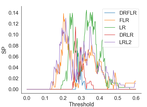
Figure 1: Evolution of SP with changes in acceptance threshold (GC)
$\rho=0.01$; $\eta=0.04$; $\kappa_{y}=\kappa_{s}=0.2$

For this reason, we also report a second fairness metric, Log Probabilistic Equalised Opportunities (LEO). This is also the measure used by the DRFLR system to penalise unfairness. Unlike SP, it does not depend on a choice of threshold. In this case, we used the difference in the expected value of the log PD of the defaults between the protected $\mathbf{\hat{y}}_{s=1,y=1}$ and non-protected $\mathbf{\hat{y}}_{s=0,y=1}$ groups.

$$LEO=\big{|}\mathbb{E}[1+ln(\mathbf{\hat{y}}_{s=1,y=1})]-\mathbb{E}[1+ln(\mathbf{\hat{y}}_{s=0,y=1})]\big{|}$$ (13)

Note that this measure focuses on fairness in the subgroup y=1; since, in credit scoring, we are especially concerned with the fairness of predicted defaults, we consider this measure to be a good fit for the purpose.

As we will argue in the following section, though, LEO tends to be over-optimistic with regularised classifiers. Hence, we will provide results not only on LEO but also on SP as part of our performance comparison. To determine the threshold, we select the optimal threshold by taking the one that maximises the difference in the true positive rate and false negative rate; this difference is often known as the Youden J statistic (Youden, 1950).

We will use k-fold cross-validation with five folds to do the train/test split. Therefore, we will divide the data into five groups, each time training the model on four of these, and test it on the remaining group (Refaeilzadeh et al., 2009). This way, we will get five classifiers for each model application and measure its performance as the average over those five out-of-sample performance values.

6 Results

This section presents numerical experiments using the five classifiers using the five credit datasets mentioned above. In addition, as DRFLR presents new and complex hyperparameters, we develop experiments for each hyperparameter and explain their effects to serve as a guide for credit scorers aiming to use DRO .

6.1 Hyperparameter tuning

The fairness penalty $\eta$ is bounded between 0 and $min(\hat{p}_{01},\hat{p}_{11})$ where $\hat{p}_{\acute{s}\acute{y}}$ is the empirical proportion of the population such that $\hat{\mathbb{P}}_{N}(s=\acute{s},y=\acute{y})$. Therefore, it is rather small in all sets, the largest being GC with $max(\eta)\approx 0.08$ and the lowest being GMSC with $max(\eta)\approx 0.001$. Indeed, in the case of GC (see Figure 2(a)), we can observe how, due to the small range, the evolution of performance in both ROC and LEO is unclear.

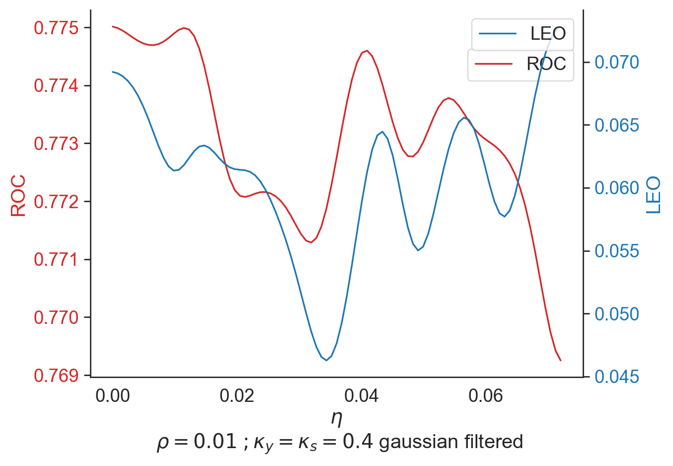
(a) changes in $\eta$

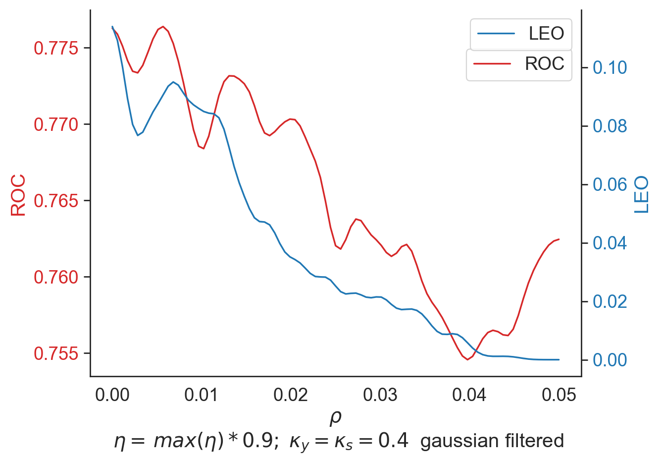
(b) changes in $\rho$

Figure 2: Evolution of ROC and LEO with changes in $\eta$ and $\rho$ (GC)

The radius of the Wasserstein ball, $\rho$, also considers the sensitive attribute in its calculation. Therefore, it is reasonable that this parameter has some effect on fairness. Furthermore, we advise being aware of the consequences of misuse of this parameter, as its performance drastically decreases with larger values. It is also worth noticing that by using grid search, we look for optimal performance. Therefore, $\rho$ will tend to be small to accommodate the distributional differences in the cross-validation splits. One should expect the deployed model to be fed with data that differs from the training, and hence, the final rho should be slightly higher than the one found during the grid search.

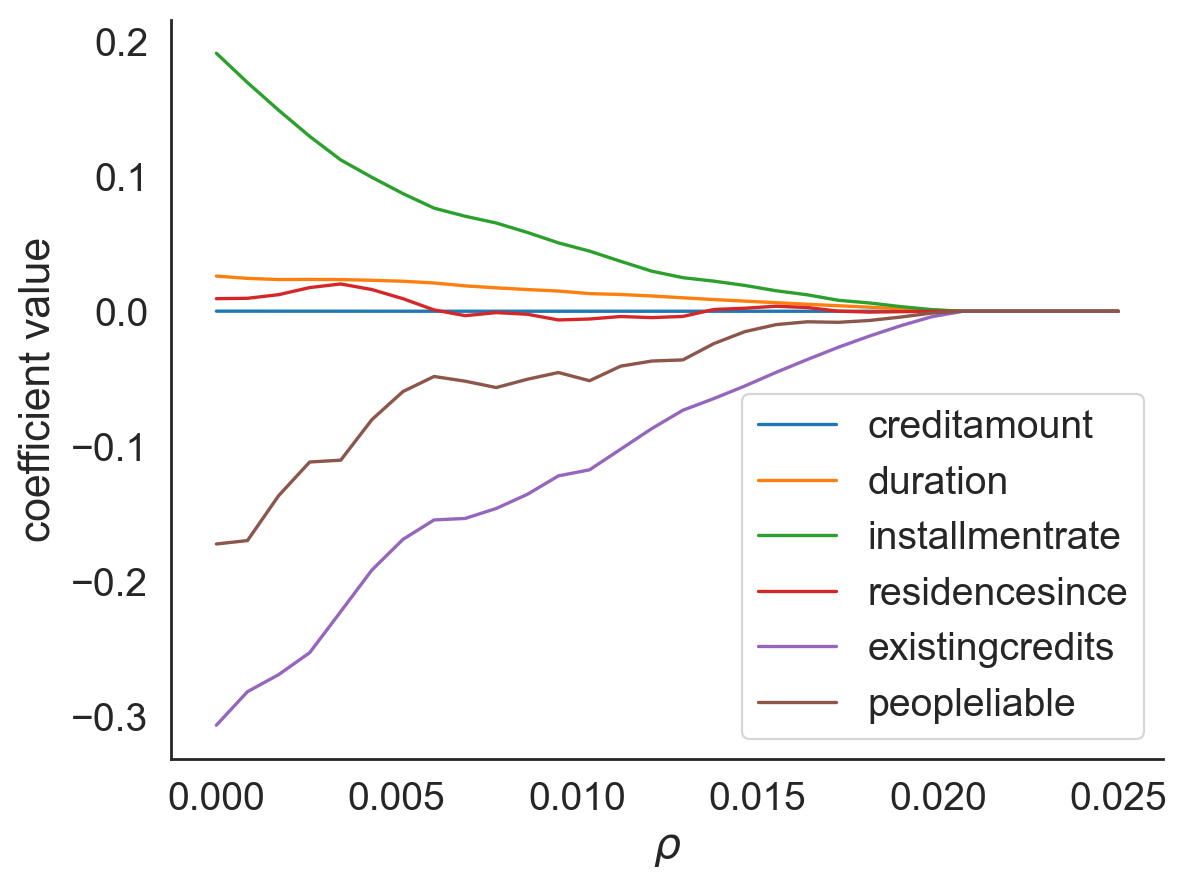
(a) Evolution of most relevant coefficients

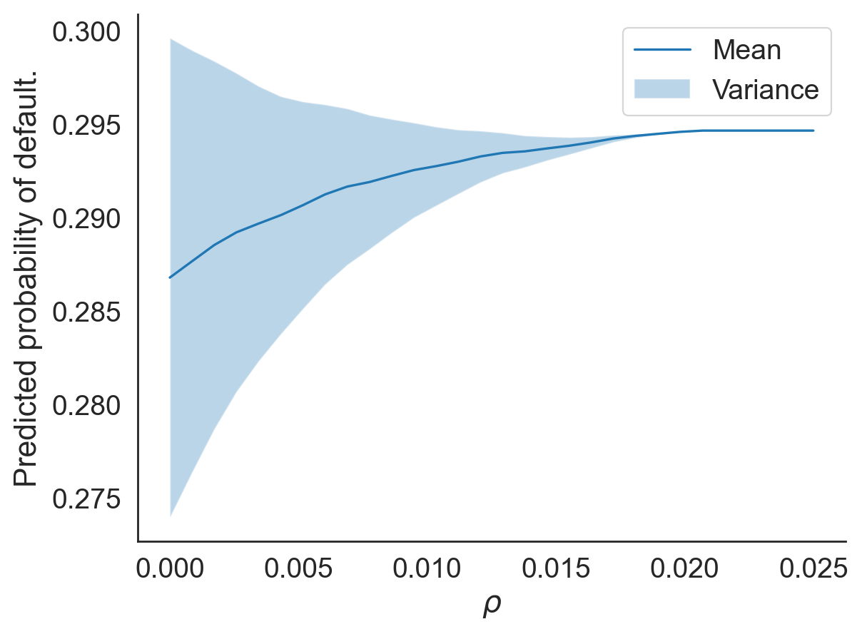
(b) Evolution of the expected PD

Figure 5: Evolution of most relevant coefficients and PD with changes in eta

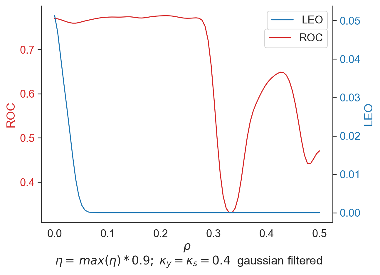
Figure 6: Evolution of ROC and LEO with changes in $\rho$ in a broader span of $\rho$ values.(GC)

Figure 2(b) shows how small changes in $\rho$ can yield large changes in LEO with a similar impact on ROC; however, good performance can be attained with near 0 LEO. Nonetheless, performance plummets rapidly after reaching a critical point (around 0.3 in the case of GC, see appendix Figure 6). As mentioned in the methods section, DRO can be viewed as a regularisation method with no assumption on the distribution family as in L1 or L2 methods. Indeed, we observe a coefficient shrinkage with this technique that produces a narrow distribution of predicted PD (appendix figure 5).

The last hyperparameters to consider are $\kappa_{y}$ and $\kappa_{s}$. The effect of $\kappa_{s}$ appears to be unclear in any scenario, as we can see from Figure 3(b). However, it is worth noticing that very low values of $\kappa_{y}$ provide the best results in terms of LEO at the expense of lower ROC. (For information on the remaining datasets, please check the supplementary material).

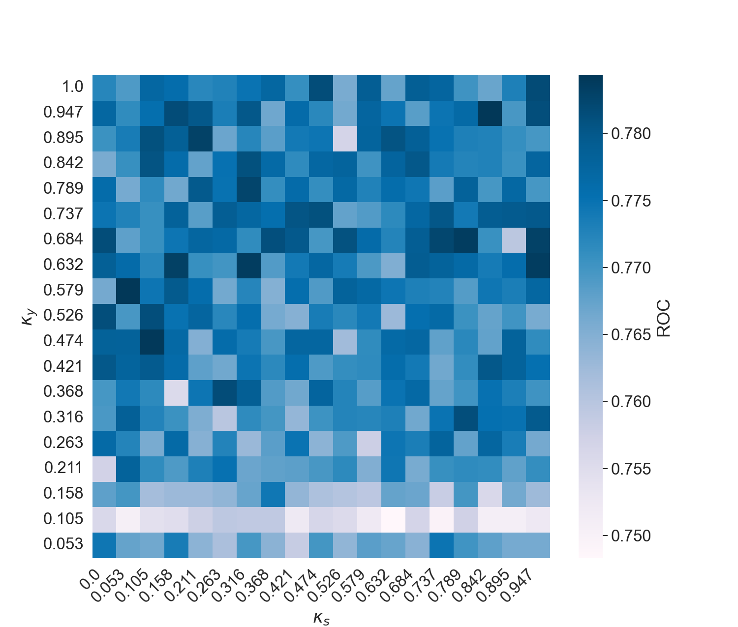
(a) ROC

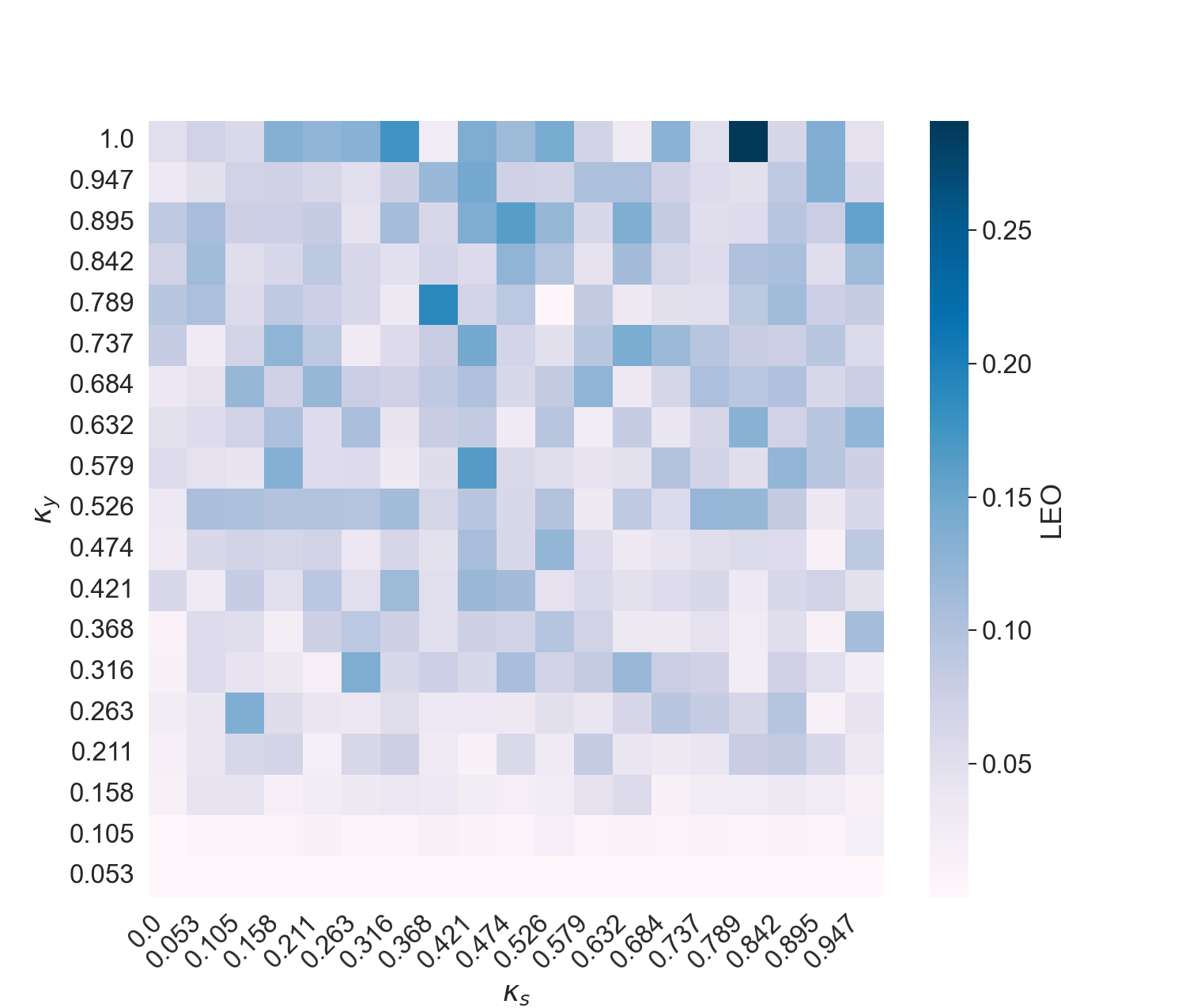
(b) LEO

Figure 3: Evolution of ROC and LEO with changes in $\kappa_{y}$ and $\kappa_{s}$ (GC)

$\rho=0.01;\;\eta=0.05$

6.2 Performance

In terms of performance, we re-iterate that due to the computational complexity of DRO, we have sub-sampled all datasets except GC, so we advise against comparing these results at face value with papers where they do not sub-sample, as reduced sample size may harm performance.

In Table 1, we can observe how DRFLR provides consistently lower LEO results with minimal loss in performance across all data sets where lower values of LEO indicate fairer treatment. In most scenarios, the close second-best performer in LEO is DRLR, which could result from an improvement in generalisation as well as the preference of LEO for regularised methods. However, it is important to note that our ground metric includes information on the sensitive attribute that may improve fairness. In terms of SP, there is no clear leader. However, DRFLR, DRLR and FLR are the top performers, indicating that fairness enhancement is not explained by lower dispersion on PD distributions alone.

Metric	Model	Datasets
		GC	HC	TC	PAKDD	GMSC
ROC	LR	0.763$\pm$0.052	0.722 $\pm$ 0.036	$0.701\pm 0.032$	$0.585\pm 0.02$	0.642$\pm$0.046
	LRL2	0.765 $\pm$ 0.052	0.723$\pm$ 0.036	$\mathbf{0.701\pm 0.031}$	$0.585\pm 0.02$	0.641$\pm$0.046
	FLR	0.764$\pm$0.052	$0.721\pm 0.036$	0.699 $\pm$ 0.034	$0.585\pm 0.02$	0.639 $\pm$ 0.043
	DRLR	0.759$\pm$0.051	$\mathbf{0.723\pm 0.032}$	0.700 $\pm$ 0.034	$0.587\pm 0.021$	0.723$\pm$ 0.046
	DRFLR	0.759$\pm$0.051	0.721$\pm$0.030	0.700 $\pm$ 0.034	$\mathbf{0.587\pm 0.021}$	0.710 $\pm$0.035
LEO	LR	$0.219\pm 0.169$	$0.778\pm 0.187$	$0.197\pm 0.140$	$0.055\pm 0.067$	$0.338\pm 0.248$
	LRL2	$0.211\pm 0.166$	$0.654\pm 0.13$	$0.196\pm 0.139$	$0.045\pm 0.066$	$0.321\pm 0.255$
	FLR	$0.204\pm 0.171$	$0.737\pm 0.210$	$0.197\pm 0.144$	$0.053\pm 0.064$	$0.332\pm 0.269$
	DRLR	$0.117\pm 0.133$	$0.01\pm 0.002$	$0.004\pm 0.011$	$\mathbf{0.002\pm 0.004}$	$2.46e^{-05}\pm 5.17e^{-05}$
	DRFLR	$\mathbf{0.088\pm 0.117}$	$\mathbf{0.002\pm 0.005}$	$\mathbf{0.001\pm 0.003}$	$0.002\pm 0.004$	$\mathbf{1.65e^{-06}\pm 2.76e^{-06}}$
SP	LR	$8.47e^{-04}\pm 0.003$	$0.007\pm 0.011$	$0.006\pm 0.019$	$0.007\pm 0.006$	$0.086\pm 0.049$
	LRL2	${8.47e^{-04}\pm 0.003}$	$0.003\pm 0.005$	$0.01\pm 0.01$	$\mathbf{0.007\pm 0.006}$	$0.094\pm 0.052$
	FLR	$\mathbf{0\pm 0}$	$\mathbf{3.39e^{-04}\pm 3.10e^{-04}}$	$0.006\pm 0.011$	$0.011\pm 0.012$	$0.083\pm 0.056$
	DRLR	$0.005\pm 0.014$	$0.003\pm 0.006$	$0.007\pm 0.01$	$0.015\pm 0.017$	$0.01\pm 0.011$
	DRFLR	$0.004\pm 0.012$	$0.007\pm 0.01$	$\mathbf{0.003\pm 0.006}$	$0.011\pm 0.019$	$\mathbf{0.01\pm 0.011}$

Table 1: Performance comparison of the selected classifiers in different credit scoring data sets
All hyperparameters tuned using grid search except $\eta$ that was fixed to 0.9*max $\eta$. Scientific notation is used when values are below 0.0005$de^{c}=d\times 10^{c}$

Finally, we do not observe drastic changes in ROC. However, it is worth noticing that the top performers are LRL2 and DRLR, indicating that robust methods can attain similar or even higher performance than heuristic methods, at least in small samples.

6.3 Changes in marginals

We will change marginal proportions in the training set to test for robustness. While this is just one type of distributional change, it does not require synthetic data. Also, it accounts for a reasonable distributional change where proportionally, more people from the protected group apply for credit than the one we have in our training data.

It is important to note that for ease of comparison, we have fixed the values of the hyperparameters. Therefore, in most cases, the algorithms have suboptimal performance. In addition, if we consider hyperparameter tunning, especially of the parameters $C$ and $\rho$ with changing population size, we expect tunning to tend to increase them with a smaller sample size.

While the general trends of all algorithms seem to be very similar, in every case, ROC resembles roughly equal using DRFLR and DRLR, while LEO and SP are consistently lower in the case for GC (4); this happened as well in the remaining datasets; check (C). In addition, those datasets show a slight tendency of LEO and SP to increase as the removed proportion increases in the non-robust classifiers. In contrast, the robust ones show stable values.

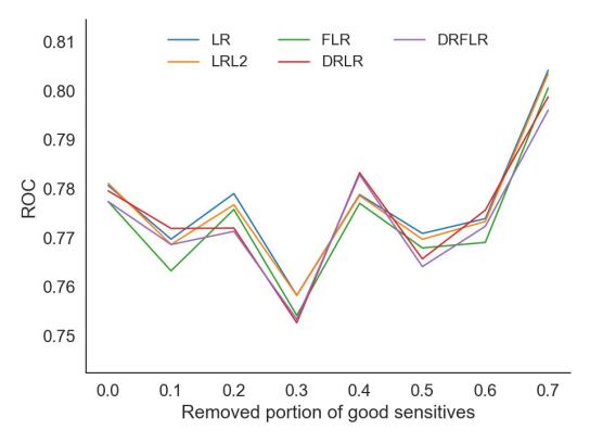
(a) ROC

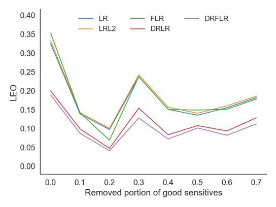
(b) LEO

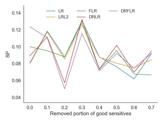
(c) SP

Figure 4: Evolution of ROC LEO and SP with changes in marginal distribution (GC)

$\rho=0.01$, $\kappa_{y}=\kappa_{s}=0.4$ $\eta=\dfrac{\max(\eta)}{1.5}$

7 Discussion and future work

Considering recent advances in developing efficient approximations of DRO (Cheramin et al., 2022; Kuhn et al., 2019), there are reasons to argue that DRO-based classifiers would be applicable to the credit industry in the future. The goal of this paper is to produce early insights into the matter. Due to the highly positive results of DRO-based classifiers in terms of LEO and their negligible or even positive impact on ROC, it is clear that DRO-based classifiers are superior to their non-robust counterparts. However, the algorithm has high computational requirements, which increase exponentially with sample size, and it cannot be parallelised, making the system, for now, ineffective in practice.

Furthermore, the experiments show a potential connection between robustness and fairness as DRLR (with no explicit fairness penalty) is often fairer than its non-robust counterparts. This indicates that increasing robustness and improving generalisation have a positive impact in terms of fairness. This connection needs separate research to be fully understood. In addition, given the importance of robustness in automated decision-making, we believe more research on the impact of the ground metric is needed, e.g. treating potential proxy features as more ambiguous than those that are not. The experiments with changes to the marginal distribution of non-default protected applicants show how DRO methods tend to perform roughly equal to their non-robust counterparts while offering better results on fairness. However, the results are insufficient to state that the DRO approach suffers significantly less from changes to the marginal distribution.

In conclusion, the use of DRO in credit scoring seems to have more advantages than disadvantages regarding its outcome. However, further research that contemplates larger data sets to provide more solid evidence is required. In addition, we argue that there is a need for unified fairness metrics for credit scoring that do not depend on the ever-changing threshold or favour low PD dispersion, as both could easily trick a regulator if carefully tweaked or selected.

Appendix A Methodology

A tractable reformulation of problem (11) has been developed by Shafieezadeh Abadeh et al. (2015), as follows.

min $$\rho\psi+\frac{1}{n}\sum_{i=1}^{n}d_{i}$$ (14)

$$\begin{aligned} \footnotesize\text{s.t.}&\quad\mathbf{w}\in\mathbb{R}^{m},\;\mathbf{d}\in\mathbb{R}^{n},\;\psi\in\mathbb{R}_{+}\normalsize\end{aligned}$$ (15)

$$\begin{aligned} \ell(x_{i},y_{i})\leq d_{i}&\quad\forall i\leq n\end{aligned}$$ (16)

$$\begin{aligned} \ell(x_{i},1-y_{i})-\psi\kappa_{y}\leq d_{i}&\quad\forall i\leq n\end{aligned}$$ (17)

$$\begin{aligned} ||\mathbf{w}||\leq\psi\end{aligned}$$ (18)

Note that as the paper by Shafieezadeh Abadeh et al. is not focused on fairness, the ground metric used for their reformulation is

$$c((\mathbf{x}_{i},y_{i}),(\mathbf{x}^{\prime}_{i},y^{\prime}_{i}))=||\mathbf{x}_{i}-\mathbf{x}^{\prime}_{i}||+\kappa_{y}|y_{i}-y^{\prime}_{i}|/2.$$

as a consequence, by setting $\kappa_{y}=\infty$ constraint(17) is always satisfied; hence, regularised LR is just one special case of DRLR.

A tractable reformulation of problem (11) has been developed by (Taskesen et al., 2020) as follows

min: $$t$$ (19)

s.t.: $$\mathbf{w}\in\mathbb{R}^{m},\psi\in\mathbb{R}_{+},d\in\mathbb{R}^{n},\mu\in\mathbb{R}^{2\times 2}\normalsize$$ (20)

$$\rho\psi+\frac{1}{n}\sum_{i=1}^{n}d_{s^{\prime}i}+\sum_{s\in\mathcal{S}}\sum_{y\in\mathcal{Y}}\hat{p}_{sy}\mu_{s^{\prime}sy}\leq t\quad\forall s^{\prime}\in[0,1]$$ (21)

$$\begin{aligned} &\|\mathbf{w}\|(1+\eta/\hat{p}_{01})\leq\psi_{0};&\quad\|\mathbf{w}\|(1+\eta/\hat{p}_{11})\leq\psi_{1}\\ \end{aligned}$$ (22)

$$\begin{aligned} &\left.\begin{aligned} &-\ln(1-h_{\mathbf{w}}(\hat{x}_{i}))-\psi\kappa_{s}|s-\hat{s}_{i}|-\psi\kappa_{y}|\hat{y}_{i}|-\mu_{s0}\leq d_{si},\\ &-\ln(1-h_{\mathbf{w}}(\hat{x}_{i}))-\psi\kappa_{s}|s^{\prime}-\hat{s}_{i}|-\psi\kappa_{y}|\hat{y}_{i}|-\mu_{s^{\prime}0}\leq d_{si},\\ &-(1-\dfrac{\eta}{\hat{p}_{s1}})\ln(h_{\mathbf{w}}(\hat{x}_{i}))-\psi\kappa_{s}|s-\hat{s}_{i}|-\psi\kappa_{y}|1-\hat{y}_{i}|-\mu_{s1}\leq d_{si},\\ &-(1-\dfrac{\eta}{\hat{p}_{s^{\prime}1}})\ln(h_{\mathbf{w}}(\hat{x}_{i}))-\psi\kappa_{s}|s^{\prime}-\hat{s}_{i}|-\psi\kappa_{y}|1-\hat{y}_{i}|-\mu_{s^{\prime}1}\leq d_{si}\end{aligned}\right)\scriptsize\begin{aligned} {\forall i\leq n}\\ {\forall s\in[0,1]}\\ s^{\prime}=s-1\end{aligned}\end{aligned}$$ (23)

where $t$ is an epigraphical variable,$d,\psi$ and $\mu$ are dual variables, and $\mathcal{Y}$ and $\mathcal{S}$ are all possible values of $\mathbf{y}$ and $\mathbf{s}$, respectively.

Appendix B Changes in $\rho$

$\kappa_{y}=\kappa_{s}=0.4;\;\eta=0.05$

Appendix C Changes in Marginal Distribution

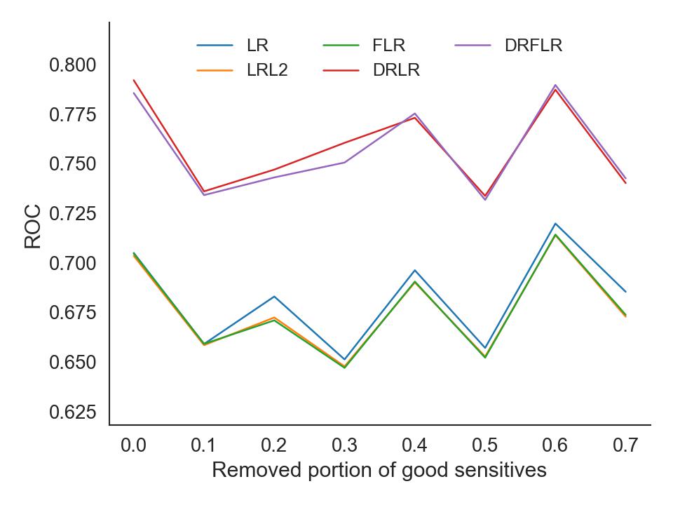
(a) GMSC

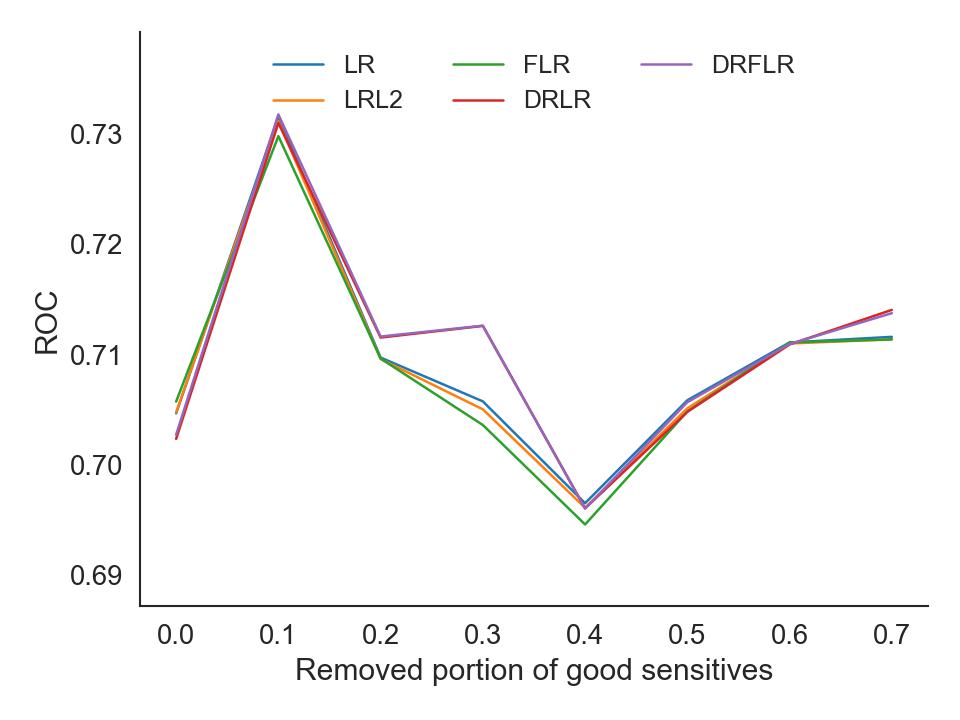
(b) HC

Figure 7: Evolution of ROC changes in marginal distribution (GMSC and HC)

$\rho=0.01$, $\kappa_{y}=\kappa_{s}=0.4$, $\eta=\frac{\max(\eta)}{1.5}$

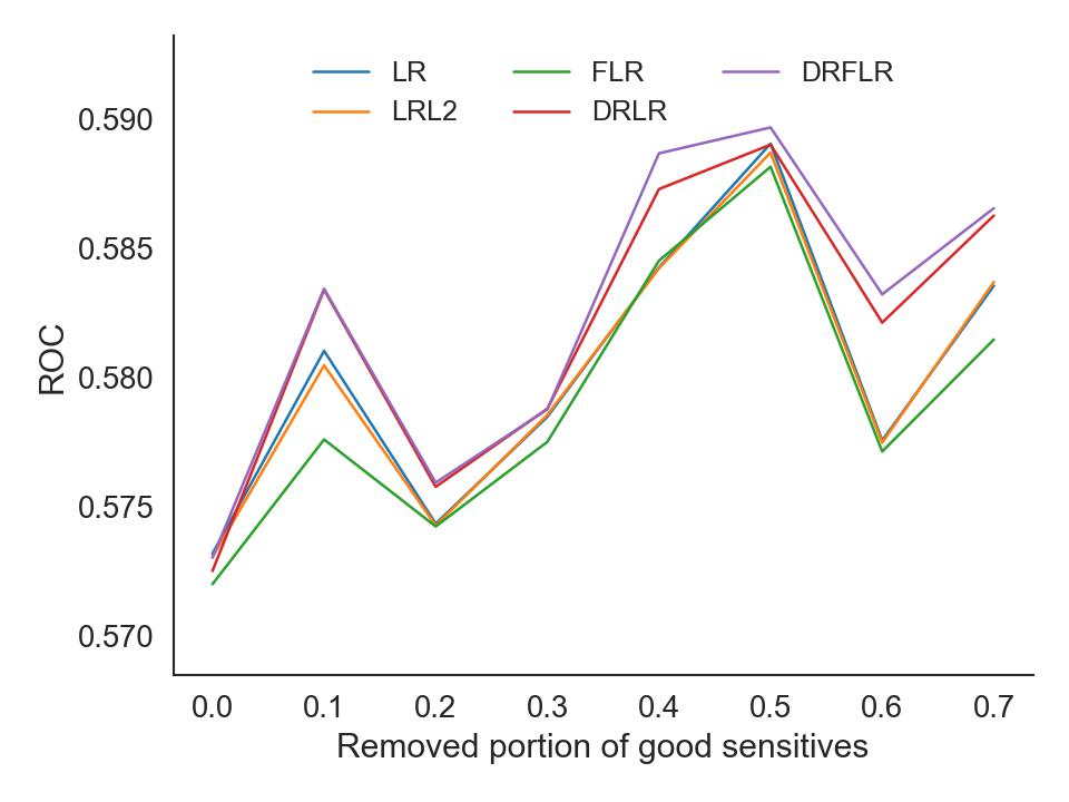
(a) PAKDD

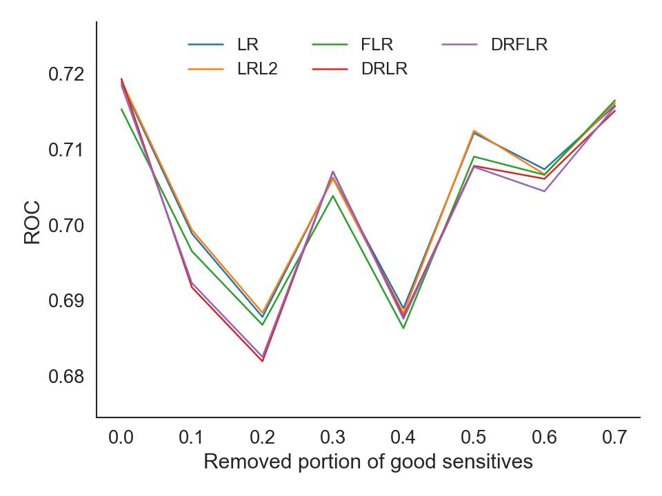
(b) TC

Figure 8: Evolution of ROC changes in marginal distribution (PAKDD and TC)

$\rho=0.01$, $\kappa_{y}=\kappa_{s}=0.4$, $\eta=\frac{\max(\eta)}{1.5}$

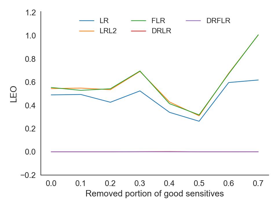
(a) GMSC

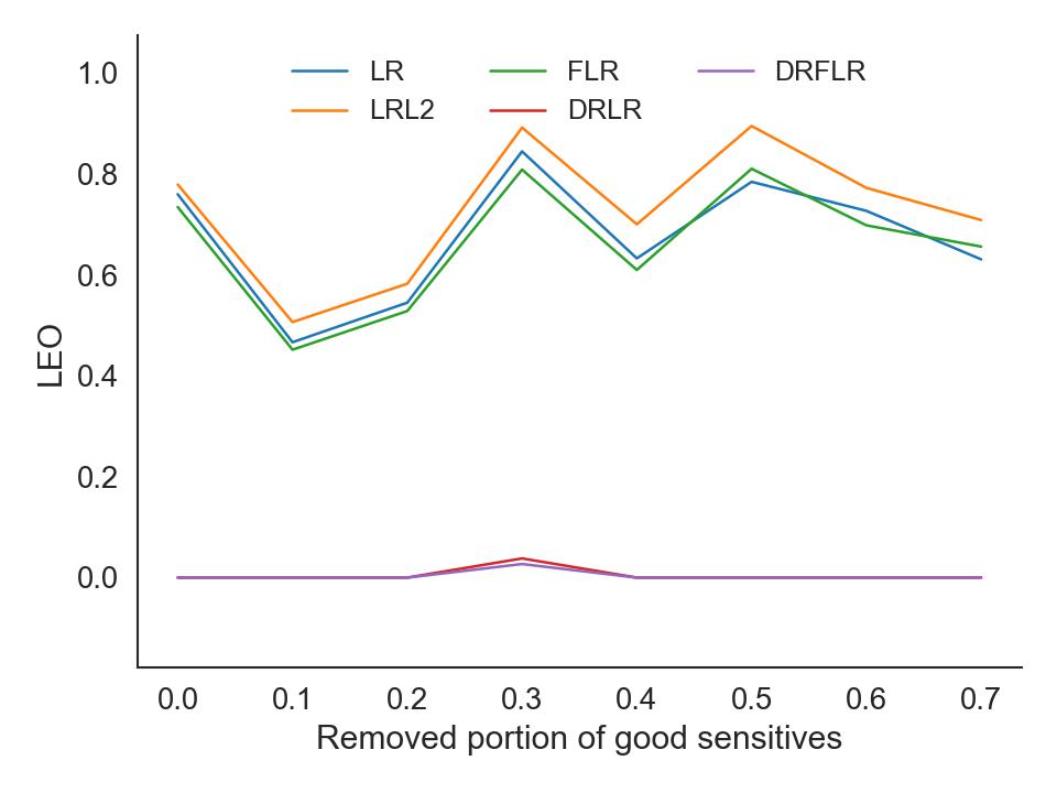
(b) HC

Figure 9: Evolution of LEO changes in marginal distribution (GMSC and HC)

$\rho=0.01$, $\kappa_{y}=\kappa_{s}=0.4$, $\eta=\frac{\max(\eta)}{1.5}$

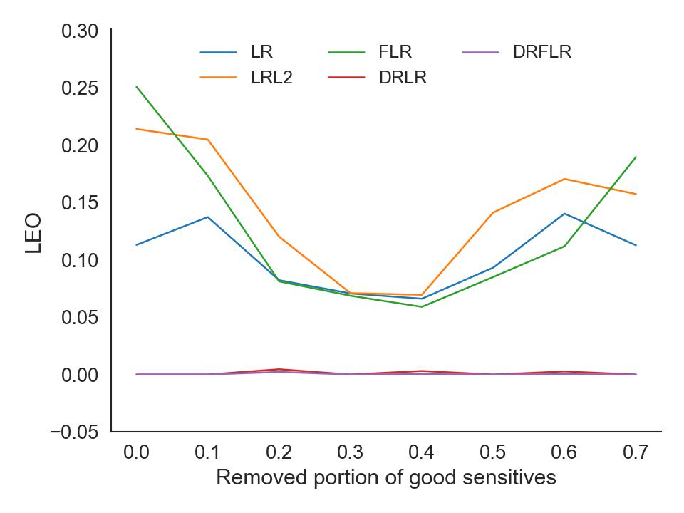
(a) PAKDD

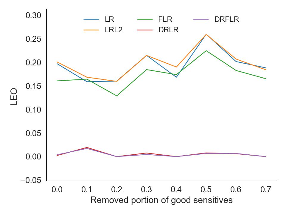
(b) TC

Figure 10: Evolution of LEO changes in marginal distribution (PAKDD and TC)

$\rho=0.01$, $\kappa_{y}=\kappa_{s}=0.4$, $\eta=\frac{\max(\eta)}{1.5}$

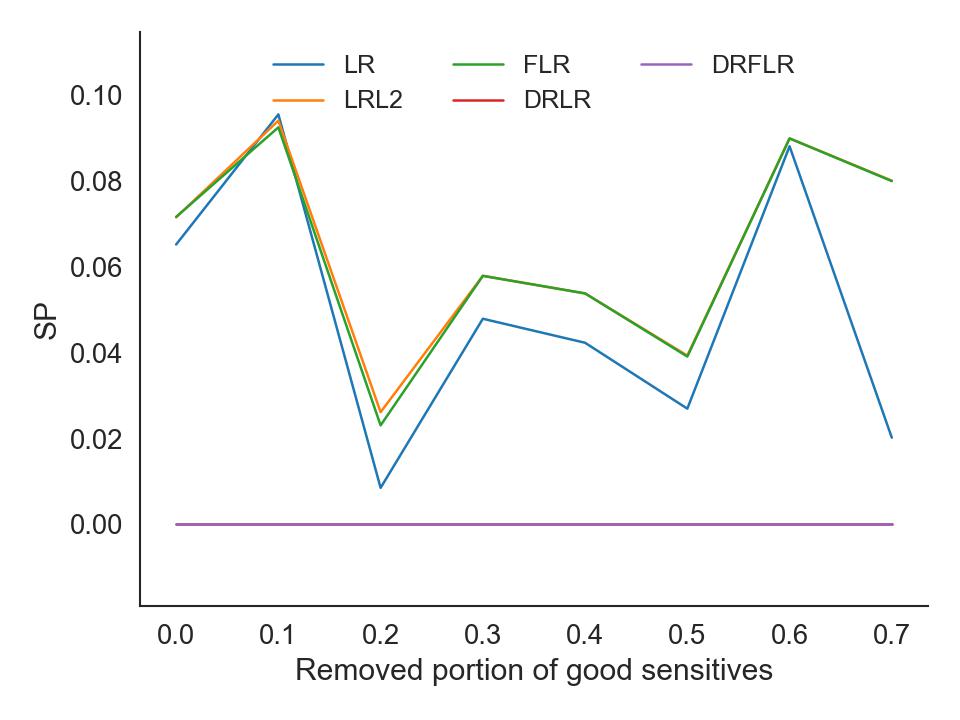
(a) GMSC

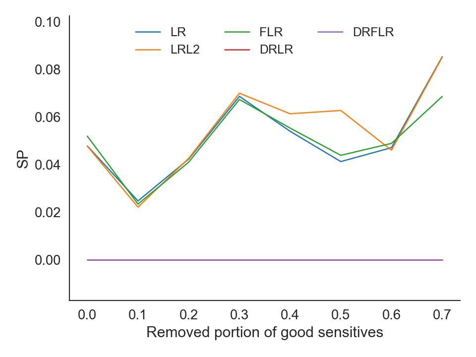
(b) HC

Figure 11: Evolution of SP changes in marginal distribution (GMSC and HC)

$\rho=0.01$, $\kappa_{y}=\kappa_{s}=0.4$, $\eta=\frac{\max(\eta)}{1.5}$

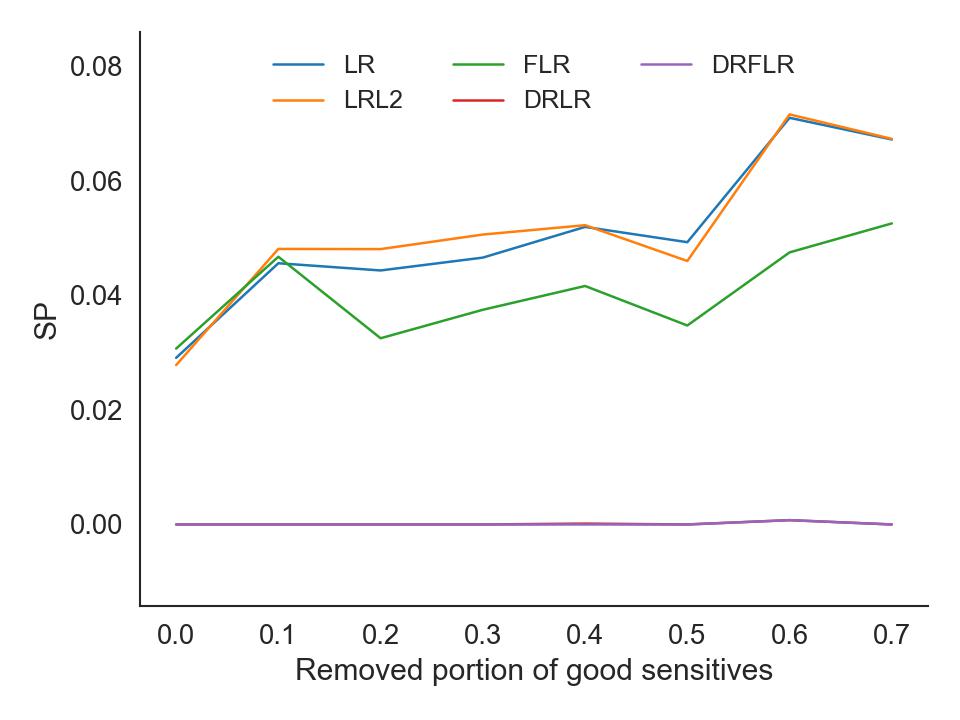
(a) PAKDD

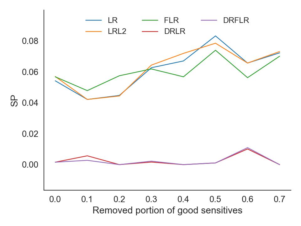
(b) TC

Figure 12: Evolution of SP changes in marginal distribution (PAKDD and TC)

$\rho=0.01$, $\kappa_{y}=\kappa_{s}=0.4$, $\eta=\frac{\max(\eta)}{1.5}$

Appendix D Data Description

Name	Description	Marginal distribution	Source
German Credit (GC)	13 categorical features, seven numerical features, 1000 instances, binary target	y=0,s=0: 0.58 y=0,s=1: 0.11 y=1,s=0: 0.23 y=1,s=1:        0.08	(Hofmann, 1994) available at the UCI Machine Learning Repository (Dua and Graff, 2017)
Give me some credit (GMSC)	12 numerical features 150 thousand samples*	y=0,s=0: 0.91 y=0,s=1: 0.02 y=1,s=0: 0.06 y=1,s=1:        0.00	(Credit Fusion, 2011) available for Kaggle competitions
Home Credit (HC)	122 numerical features 308 thousand samples*	y=0,s=0: 0.88 y=0,s=1: 0.04 y=1,s=0: 0.08 y=1,s=1:        0.01	(Anna Montoya, 2018) available for Kaggle competitions
Taiwan Credit (TC)	24 numerical features 30 thousand samples*	y=0,s=0: 0.68 y=0,s=1: 0.09 y=1,s=0: 0.19 y=1,s=1:       0.04	(I-Cheng, 2016) available at the UCI Machine Learning Repository (Dua and Graff, 2017)
Pacific-Asia Knowledge Discovery and Data Mining Conference (PAKDD)	52 numerical features 50 thousand samples*	y=0,s=0: 0.67 y=0,s=1: 0.08 y=1,s=0: 0.21 y=1,s=1:        0.04	(Aligam, 2010) available for competitions

Table 2: Datasets List and Description
Sub-sampled to 5000 with equal marginal distributions on y and s due to lack of computational power available and absence of parallelisation capability

References

- Aligam (2010) Aligam, E., 2010. The 14th pacific-asia conference on knowledge discovery and data mining. URL: https://pakdd.org/archive/pakdd2010/PAKDDCompetition.html.
- Andreeva and Matuszyk (2019) Andreeva, G., Matuszyk, A., 2019. The law of equal opportunities or unintended consequences?: The effect of unisex risk assessment in consumer credit. Journal of the Royal Statistical Society: Series A (Statistics in Society) 182, 1287–1311.
- Anna Montoya (2018) Anna Montoya, inversion KirillOdintsov, M.K., 2018. Home credit default risk. URL: https://kaggle.com/competitions/home-credit-default-risk.
- Barocas et al. (2017) Barocas, S., Hardt, M., Narayanan, A., 2017. Fairness in machine learning. Nips tutorial 1, 2.
- Ben-Tal et al. (2009) Ben-Tal, A., El Ghaoui, L., Nemirovski, A., 2009. Robust optimization. volume 28. Princeton university press.
- Ben-Tal and Nemirovski (1998) Ben-Tal, A., Nemirovski, A., 1998. Robust convex optimization. Mathematics of operations research 23, 769–805.
- Bertsimas and Sim (2004) Bertsimas, D., Sim, M., 2004. The price of robustness. Operations research 52, 35–53.
- Blanchet et al. (2019) Blanchet, J., Kang, Y., Murthy, K., 2019. Robust wasserstein profile inference and applications to machine learning. Journal of Applied Probability 56, 830–857.
- Calders et al. (2009) Calders, T., Kamiran, F., Pechenizkiy, M., 2009. Building classifiers with independency constraints, in: 2009 IEEE International Conference on Data Mining Workshops, IEEE. pp. 13–18.
- Cheramin et al. (2022) Cheramin, M., Cheng, J., Jiang, R., Pan, K., 2022. Computationally efficient approximations for distributionally robust optimization under moment and wasserstein ambiguity. INFORMS Journal on Computing 34, 1768–1794.
- Chouldechova (2017) Chouldechova, A., 2017. Fair prediction with disparate impact: A study of bias in recidivism prediction instruments. Big data 5, 153–163.
- Chouldechova and Roth (2018) Chouldechova, A., Roth, A., 2018. The frontiers of fairness in machine learning. arXiv preprint arXiv:1810.08810 .
- Credit Fusion (2011) Credit Fusion, W.C., 2011. Give me some credit. URL: https://kaggle.com/competitions/GiveMeSomeCredit.
- Cuturi and Avis (2014) Cuturi, M., Avis, D., 2014. Ground metric learning. The Journal of Machine Learning Research 15, 533–564.
- Dua and Graff (2017) Dua, D., Graff, C., 2017. UCI machine learning repository. URL: http://archive.ics.uci.edu/ml.
- Dwork et al. (2012) Dwork, C., Hardt, M., Pitassi, T., Reingold, O., Zemel, R., 2012. Fairness through awareness, in: Proceedings of the 3rd innovations in theoretical computer science conference, pp. 214–226.
- Falque-Pierrotin (2017) Falque-Pierrotin, I., 2017. Guidelines on data protection officers (’dpos’). URL: https://ec.europa.eu/newsroom/article29/items/612048/en.
- Gao et al. (2022) Gao, R., Chen, X., Kleywegt, A.J., 2022. Wasserstein distributionally robust optimization and variation regularization. Operations Research .
- Garcia-Escribano and Han (2015) Garcia-Escribano, M.M., Han, M.F., 2015. Credit expansion in emerging markets: propeller of growth? International Monetary Fund.
- Hardt et al. (2016a) Hardt, M., Price, E., Price, E., Srebro, N., 2016a. Equality of opportunity in supervised learning, in: Lee, D., Sugiyama, M., Luxburg, U., Guyon, I., Garnett, R. (Eds.), Advances in Neural Information Processing Systems, Curran Associates, Inc.. p. 3323–3331. URL: https://proceedings.neurips.cc/paper_files/paper/2016/file/9d2682367c3935defcb1f9e247a97c0d-Paper.pdf.
- Hardt et al. (2016b) Hardt, M., Price, E., Srebro, N., 2016b. Equality of opportunity in supervised learning. Advances in neural information processing systems 29.
- Hofmann (1994) Hofmann, H., 1994. Statlog (german credit data) data set. URL: https://archive.ics.uci.edu/ml/datasets/statlog+(german+credit+data).
- I-Cheng (2016) I-Cheng, Y., 2016. default of credit card clients data set. URL: https://archive.ics.uci.edu/ml/datasets/default+of+credit+card+clients.
- Kamiran and Calders (2009) Kamiran, F., Calders, T., 2009. Classifying without discriminating, in: 2009 2nd international conference on computer, control and communication, IEEE. pp. 1–6.
- Kamiran et al. (2012) Kamiran, F., Karim, A., Zhang, X., 2012. Decision theory for discrimination-aware classification, in: 2012 IEEE 12th International Conference on Data Mining, IEEE. pp. 924–929.
- Kamishima et al. (2011) Kamishima, T., Akaho, S., Sakuma, J., 2011. Fairness-aware learning through regularization approach, in: 2011 IEEE 11th International Conference on Data Mining Workshops, IEEE. pp. 643–650.
- Kantorovich (1960) Kantorovich, L.V., 1960. Mathematical methods of organizing and planning production. Management science 6, 366–422.
- Kozodoi et al. (2022) Kozodoi, N., Jacob, J., Lessmann, S., 2022. Fairness in credit scoring: Assessment, implementation and profit implications. European Journal of Operational Research 297, 1083–1094.
- Krempl and Hofer (2011) Krempl, G., Hofer, V., 2011. Classification in presence of drift and latency, in: 2011 IEEE 11th International Conference on Data Mining Workshops, IEEE. pp. 596–603.
- Kuhn et al. (2019) Kuhn, D., Esfahani, P.M., Nguyen, V.A., Shafieezadeh-Abadeh, S., 2019. Wasserstein distributionally robust optimization: Theory and applications in machine learning, in: Operations Research & Management Science in the Age of Analytics. INFORMS, pp. 130–166.
- Lessmann et al. (2015) Lessmann, S., Baesens, B., Seow, H.V., Thomas, L.C., 2015. Benchmarking state-of-the-art classification algorithms for credit scoring: An update of research. European Journal of Operational Research 247, 124–136.
- Li et al. (2019) Li, J., Huang, S., So, A.M.C., 2019. A first-order algorithmic framework for distributionally robust logistic regression. Advances in Neural Information Processing Systems 32.
- Long et al. (2023) Long, D.Z., Sim, M., Zhou, M., 2023. Robust satisficing. Operations Research 71, 61–82.
- Martinez-Plumed et al. (2019) Martinez-Plumed, F., Ferri, C., Nieves, D., Hernandez-Orallo, J., 2019. Fairness and missing values. arXiv preprint arXiv:1905.12728 .
- Moscato et al. (2021) Moscato, V., Picariello, A., Sperli, G., 2021. A benchmark of machine learning approaches for credit score prediction. Expert Systems with Applications 165, 113986.
- Murphy (2012) Murphy, K.P., 2012. Machine learning: a probabilistic perspective. MIT press.
- Muñoz et al. (2016) Muñoz, C., Smith, M., Patil, D., 2016. Big data: A report on algorithmic systems, opportunity and civil rights. URL: https://obamawhitehouse.archives.gov/sites/default/files/microsites/ostp/2016_0504_data_discrimination.pdf.
- Netrapalli (2019) Netrapalli, P., 2019. Stochastic gradient descent and its variants in machine learning. Journal of the Indian Institute of Science 99, 201–213.
- Ovadia et al. (2019) Ovadia, Y., Fertig, E., Ren, J., Nado, Z., Sculley, D., Nowozin, S., Dillon, J., Lakshminarayanan, B., Snoek, J., 2019. Can you trust your model’s uncertainty? evaluating predictive uncertainty under dataset shift. Advances in neural information processing systems 32.
- Pessach and Shmueli (2020) Pessach, D., Shmueli, E., 2020. Algorithmic fairness. arXiv preprint arXiv:2001.09784 .
- Rahimian and Mehrotra (2019) Rahimian, H., Mehrotra, S., 2019. Distributionally robust optimization: A review. arXiv preprint arXiv:1908.05659 .
- Refaeilzadeh et al. (2009) Refaeilzadeh, P., Tang, L., Liu, H., 2009. Cross-validation. Encyclopedia of database systems 5, 532–538.
- Salehi et al. (2019) Salehi, F., Abbasi, E., Hassibi, B., 2019. The impact of regularization on high-dimensional logistic regression. arXiv preprint arXiv:1906.03761 .
- Selbst (2017) Selbst, A.D., 2017. Disparate impact in big data policing. Ga. L. Rev. 52, 109.
- Shafieezadeh Abadeh (2020) Shafieezadeh Abadeh, S., 2020. Wasserstein Distributionally Robust Learning. Technical Report. EPFL.
- Shafieezadeh Abadeh et al. (2015) Shafieezadeh Abadeh, S., Mohajerin Esfahani, P.M., Kuhn, D., 2015. Distributionally robust logistic regression. Advances in Neural Information Processing Systems 28.
- Soyster (1973) Soyster, A.L., 1973. Convex programming with set-inclusive constraints and applications to inexact linear programming. Operations research 21, 1154–1157.
- Subbaswamy et al. (2021) Subbaswamy, A., Adams, R., Saria, S., 2021. Evaluating model robustness and stability to dataset shift, in: International Conference on Artificial Intelligence and Statistics, PMLR. pp. 2611–2619.
- Taskesen et al. (2020) Taskesen, B., Nguyen, V.A., Kuhn, D., Blanchet, J., 2020. A distributionally robust approach to fair classification. arXiv preprint arXiv:2007.09530 .
- Thomas et al. (2002) Thomas, L.c., Edelman, D.B., Croock, J.N., 2002. Credit scoring and its applications. Society for Industrial and Applied Mathematics.
- Tian and Zhang (2022) Tian, Y., Zhang, Y., 2022. A comprehensive survey on regularization strategies in machine learning. Information Fusion 80, 146–166.
- Tibshirani (1996) Tibshirani, R., 1996. Regression shrinkage and selection via the lasso. Journal of the Royal Statistical Society Series B: Statistical Methodology 58, 267–288.
- Wang et al. (2020) Wang, and Guo, W., Narasimhan, H., Cotter, A., Gupta, M., Jordan, M., 2020. Robust optimization for fairness with noisy protected groups. Advances in Neural Information Processing Systems 33, 5190–5203.
- Wang et al. (2021) Wang, Y., Nguyen, V.A., Hanasusanto, G.A., 2021. Wasserstein robust classification with fairness constraints. arXiv preprint arXiv:2103.06828 .
- Xu et al. (2010) Xu, H., Caramanis, C., Mannor, S., 2010. Robust regression and lasso. IEEE Transactions on Information Theory 56, 3561–3574.
- Ying (2019) Ying, X., 2019. An overview of overfitting and its solutions, in: Journal of physics: Conference series, IOP Publishing. p. 022022.
- Youden (1950) Youden, W.J., 1950. Index for rating diagnostic tests. Cancer 3, 32–35.
- Zhang et al. (2007) Zhang, D., Huang, H., Chen, Q., Jiang, Y., 2007. A comparison study of credit scoring models, in: Third International Conference on Natural Computation (ICNC 2007), IEEE. pp. 15–18.
- Zliobaite et al. (2016) Zliobaite, I., Pechenizkiy, M., Gama, J., 2016. An overview of concept drift applications. Big data analysis: new algorithms for a new society , 91–114.