Misspecification uncertainties in near-deterministic regression

Abstract

The expected loss is an upper bound to the model generalization error which admits robust PAC-Bayes bounds for learning. However, loss minimization is known to ignore misspecification, where models cannot exactly reproduce observations. This leads to significant underestimates of parameter uncertainties in the large data, or underparameterized, limit. We analyze the generalization error of near-deterministic, misspecified and underparametrized surrogate models, a regime of broad relevance in science and engineering. We show posterior distributions must cover every training point to avoid a divergent generalization error and derive an ensemble ansatz that respects this constraint, which for linear models incurs minimal overhead. The efficient approach is demonstrated on model problems before application to high dimensional datasets in atomistic machine learning. Parameter uncertainties from misspecification survive in the underparametrized limit, giving accurate prediction and bounding of test errors.

I Introduction

Surrogate models are widely used across science and engineering, notably to efficiently approximate the action of computationally intensive simulation engines  (Alizadeh et al., 2020; Deringer et al., 2019; Lapointe et al., 2020; Nyshadham et al., 2019; Montes de Oca Zapiain et al., 2022; Bonatti et al., 2022). Domain expertise is leveraged to design optimal features and model architecture before parameter inference is carried out based on training data generated by the engines. In this paper, we consider the common scenario where the learning problems share three key characteristics:

• simulation engines are near deterministic: simulation outputs have vanishing aleatoric uncertainty. For example, the atomic energy $V({\bf X})$ is a deterministic function of atomic positions ${\bf X}$.

• surrogate models are misspecified: no single choice of the $P$ model parameters can match all $N$ training observations, such that model averaging is required to capture uncertainties.

• surrogate models are underparametrized ($N$$\gg$$P$): large quantities of training data are available, such that standard Bayesian regression schemes give vanishing parameter uncertainties.

Misspecification affects both finite capacity models and deep learning approaches with finite training resources  (Lahlou et al., 2021; Psaros et al., 2023). A misspecification-aware learning scheme should minimize the cross entropy between predicted and observed data distributions, known as the generalization error or predictive risk (see (Alquier, 2021; Morningstar et al., 2022)), but this loss is typically numerically intractable for high dimensional models.
Bayesian learning schemes instead minimize the expected loss (log likelihood), an upper bound to the generalization error, which is known to ignore misspecification. Epistemic uncertainties are therefore typically severely underestimated and can be shown to vanish in the underparametrized limit, with broad implications for surrogate model selection, uncertainty quantification and error propagation, as noted by multiple groups (Masegosa, 2020; Kato et al., 2022; Lotfi et al., 2022; Lahlou et al., 2021; Psaros et al., 2023; Imbalzano et al., 2021). We analyze the generalization error of deterministic, misspecified and under-parametrized surrogate models, i.e. those typically used to approximate simulation engines in science and engineering. The deterministic limit is atypical in Bayesian analysis, as log likelihoods are typically required to be bounded and smooth, requiring a finite aleatoric uncertainty. Here, we take the deterministic limit to derive conditions that any parameter distribution must obey to avoid a divergent generalization error, then derive a simple ensemble ansatz which admits a robust learning scheme. Our main contributions are:

• We define a pointwise optimal parameter sets (POPS) for each training point, for which model predictions are exact. Parameter distributions must have mass in every POPS to avoid a divergent generalization error. An ensemble ansatz is proposed that respects POPS occupancy and gives a finite generalization error.

• For linear models, our ansatz can be efficiently evaluated via rank-one updates to a leverage-weighted loss minimizer. This is our main result, an efficient scheme to incorporate misspecification into linear regression with minimal computational overhead.

• We compare our ansatz to direct numerical minimization of the generalization error, showing how our scheme provides robust bounds on test errors. This is confirmed in numerical experiments on challenging datasets from atomic machine learning.

(Germain et al., 2016) established an important connection between Bayesian inference and probability approximately correct (PAC-Bayes) analysis, which bounds true expectations by empirical likelihood expectations through concentration inequalities. This provides a robust learning scheme without test-train splitting, and gives a rationalization for Bayesian inference as a form of regularization. In particular, minimizing the PAC-Bayes bound for the expected loss gives the familiar relation between posterior, prior and likelihood from Bayesian inference.

In recent years, multiple groups have used the PAC-Bayes framework to derive tighter bounds for the generalization error than that provided by the expected loss  (Masegosa, 2020; Germain et al., 2016; Lahlou et al., 2021; Psaros et al., 2023; Lotfi et al., 2022; Morningstar et al., 2022). However, these efforts focus on probabilistic regression settings, often with neural network models far from the underparametrized limit, meaning aleatoric, epistemic and misspecification errors must be considered jointly.

(Masegosa, 2020) derived second order PAC-Bayes bounds for the generalization error, minimized through a variational or ensemble ansatz. (Morningstar et al., 2022) developed estimators to assess disagreement between the generalization error and expected loss, deriving specialized PAC bounds for theoretical guarantees. (Lahlou et al., 2021) considered misspecification of neural networks, jointly training a minimum loss surrogate and an independent predictor of misspecification error. (Lotfi et al., 2022) considered misspecification in the context of deep model selection, deriving conditional likelihoods better aligned with the generalization error.

As misspecification has received only recent attention in the literature, various definitions for the distinction between epistemic and misspecification uncertainties exist (Kato et al., 2022). Here, misspecification is defined as non-aleatoric uncertainties which survive in the underparametrized limit $N/P\to\infty$, where PAC-Bayes bounds for the expected loss become tight. Our epistemic uncertainties thus coincide with standard estimates from loss minimization.

II Bayesian surrogate models

II.1 Deterministic Simulation Engines

A simulation engine ${\mathcal{E}}:{\mathcal{X}}\to{\mathcal{Y}}$ takes input ${\mathbf{X}}\in{\mathcal{X}}$ and returns ${\mathbf{Y}}\in{\mathcal{Y}}$. We denote the dimension of ${\mathcal{Y}}$ and ${\mathcal{X}}$ by $Y$ and $X$ respectively. We consider the regime where the aleatoric uncertainty of ${\mathcal{E}}$ is weak and can be described as a Gaussian distribution with mean $\langle{\mathbf{Y}}|{\mathbf{X}}\rangle\equiv{\mathcal{E}}({\mathbf{X}})$ and covariance $\langle{\mathbf{Y}}\otimes{\mathbf{Y}}|{\mathbf{X}}\rangle-{\mathcal{E}}({\mathbf{X}})\otimes{\mathcal{E}}({\mathbf{X}})\equiv{\bm{\Sigma}}_{\mathcal{Y}}({\mathbf{X}})$, where $\|{\bm{\Sigma}}_{\mathcal{Y}}({\mathbf{X}})\|=\mathcal{O}(\epsilon^{2Y})$, and $\epsilon$ is assumed small. The true conditional output distribution thus reads

$$\rho_{\mathcal{E}}({\mathbf{Y}}|{\mathbf{X}})=\mathcal{N}({\mathbf{Y}}|{\mathcal{E}}({\mathbf{X}}),{\bm{\Sigma}}_{\mathcal{Y}}({\mathbf{X}})).$$ (1)

We assume homoskedatiscity ${\bm{\Sigma}}_{\mathcal{Y}}({\mathbf{X}})={\bm{\Sigma}}_{\mathcal{Y}}$ of this weak aleatoric error to investigate the deterministic, underparametrised limit $\epsilon\to 0$, $N/P\to\infty$ for $\epsilon=\mathcal{O}(\sqrt{P/N})$. With weights $\sum_{i=1}^{N}{\rm w}_{i}=1$, the training configurations ${\mathcal{D}}_{N}=\{{\mathbf{X}}_{i}\}_{i=1}^{N}$ form an input distribution

$$\rho_{N}({\mathbf{X}})\equiv\sum_{i}{\rm w}_{i}\delta({\mathbf{X}}-{\mathbf{X}}_{i}),\,\,\rho_{{\mathcal{D}}}({\mathbf{X}})\equiv\lim_{N\to\infty}\rho_{N}({\mathbf{X}}).$$ (2)

The non-parametric estimate of $\rho_{N}$ will suffer from a curse of dimensionality (Tsybakov, 2008), i.e. the worst case error scales as $N^{1/(1+{\rm Dim}({\mathbf{X}}))}$$\simeq$1. However, learning only requires that we can bound expectations over independent identically distributed (i.i.d.) samples ${\mathbf{X}},{\mathbf{Y}}\in{\mathcal{D}}$

$$\langle f({\mathbf{Y}},{\mathbf{X}})\rangle_{{\mathcal{D}}}\equiv\int_{\mathcal{D}}f({\mathbf{Y}},{\mathbf{X}})\rho_{\mathcal{E}}({\mathbf{Y}}|{\mathbf{X}})\rho_{{\mathcal{D}}}({\mathbf{X}}){\rm d}{\mathbf{X}}{\rm d}{\mathbf{Y}}.$$ (3)

For timeseries or other signal data the i.i.d. property is only satisfied for decorrelated segments ${\mathbf{X}}=\{{\bf x}_{t}\}_{t=1}^{T}$, meaning ${\bm{\Sigma}}_{\mathcal{Y}}({\mathbf{X}})$ captures signal correlations as in generalized least squares regression.

II.2 Deterministic Surrogate Models and the Generalization Error

A surrogate model ${\mathcal{M}}:{\mathcal{X}}\to{\mathcal{Y}}$ for ${\mathcal{E}}$ is defined by $P$ parameters ${\bm{\Theta}}\in{\mathcal{P}}$. Under a parameter distribution $\pi({\bm{\Theta}})$, the predicted distribution has the same form as (1), reading

$$\rho_{\mathcal{M}}({\mathbf{Y}}|{\mathbf{X}},{\bm{\Theta}}) =\mathcal{N}({\mathbf{Y}}|{\mathcal{M}}({\mathbf{X}},{\bm{\Theta}}),{\bm{\Sigma}}_{\mathcal{Y}}),$$ (4)

$$\rho_{\mathcal{M}}({\mathbf{Y}}|{\mathbf{X}}) =\int_{\mathcal{P}}\rho_{\mathcal{M}}({\mathbf{Y}}|{\mathbf{X}},{\bm{\Theta}})\pi({\bm{\Theta}}){\rm d}{\bm{\Theta}}.$$ (5)

Unlike typical Bayesian schemes, we do not treat the covariance term ${\bm{\Sigma}}_{\mathcal{Y}}$ as fitting parameter but as an intrinsic property of the quasi-deterministic simulation engine ${\mathcal{E}}$. This has implications for model selection criteria, as we discuss in appendix A.

The generalization error ${\mathcal{G}}[\pi]$ is simply the cross entropy of predicted to observed distributions. The $\rho_{N}({\mathbf{X}})$ terms cancel inside the log and, omiting the constant ${\mathcal{G}}_{\mathcal{E}}\equiv\left\langle\ln\left|\rho_{\mathcal{E}}({\mathbf{Y}}|{\mathbf{X}})\right|\right\rangle_{\mathcal{D}}$, we have

$${\mathcal{G}}[\pi]=-\left\langle\ln\left|\int_{\mathcal{P}}\rho_{\mathcal{M}}({\mathbf{Y}}|{\mathbf{X}},{\bm{\Theta}})\pi({\bm{\Theta}}){\rm d}{\bm{\Theta}}\right|\right\rangle_{\mathcal{D}},$$ (6)

PAC-Bayes analysis (Alquier, 2021) provides concentration inequalities (Hoeffding, 1994) that bound expectations (3) over ${\mathcal{D}}$ by empirical expectations over ${\mathcal{D}}_{N}$. These require $f({\mathbf{Y}},{\mathbf{X}})$ to be bounded (i.e. $\epsilon>0$) and expressed as an expectation over $\pi({\bm{\Theta}})$, i.e. $f({\mathbf{Y}},{\mathbf{X}})=\int_{\mathcal{P}}f({\mathbf{Y}},{\mathbf{X}},{\bm{\Theta}})\pi({\bm{\Theta}}){\rm d}{\bm{\Theta}}$. As ${\mathcal{G}}[\pi]$ is not in this form, PAC concentration inequalities can only be applied to some upper bound for ${\mathcal{G}}[\pi]$ which is an expectation over $\pi({\bm{\Theta}})$.

II.3 The expected loss and PAC estimation

The bound used in Bayesian schemes is for the expected loss ${\mathcal{L}}[\pi]\geq{\mathcal{G}}[\pi]$, often known as the negative log likelihood. The Jensen inequality for convex functions $f(\langle x\rangle)\leq\langle f(x)\rangle$ gives, with $f(x)=-\ln|x|$,

$$\mathcal{G}[\pi]\leq{\mathcal{L}}[\pi]=-\int_{\mathcal{P}}\left\langle\ln\left|\rho_{\mathcal{M}}({\mathbf{Y}}|{\mathbf{X}},{\bm{\Theta}})\right|\right\rangle_{\mathcal{D}}\pi({\bm{\Theta}}){\rm d}{\bm{\Theta}}.$$ (7)

The empirical expected loss $\hat{{\mathcal{L}}}_{N}[\pi]$ over $\rho_{N}({\mathbf{X}})$ can estimate the true expected loss ${\mathcal{L}}[\pi]$ through the PAC-Bayes concentration inequality, as shown by (Germain et al., 2016)

$${\mathcal{L}}[\pi]\leq\hat{{\mathcal{L}}}_{N}[\pi] \equiv\int_{\mathcal{P}}\hat{L}_{N}({\bm{\Theta}})\pi({\bm{\Theta}}){\rm d}{\bm{\Theta}}$$

$$+\frac{1}{N}\int_{\mathcal{P}}\ln\left|\frac{\pi({\bm{\Theta}})}{\pi_{0}({\bm{\Theta}})}\right|\pi({\bm{\Theta}}){\rm d}{\bm{\Theta}}+\frac{C_{0}}{N}$$ (8)

where $\hat{L}_{N}({\bm{\Theta}})=-\langle\ln|\rho_{\mathcal{M}}({\mathbf{Y}}|{\mathbf{X}},{\bm{\Theta}})|\rangle_{N}$ is the empirical loss over $\rho_{N}({\mathbf{X}})$, the distribution $\pi_{0}({\bm{\Theta}})$ is to some prior and $C_{0}$ is independent of $\pi$ but depends on $\epsilon$ and $\pi_{0}$. A well chosen prior thus tightens the PAC bound. Minimization of $\hat{{\mathcal{L}}}_{N}[\pi]$ yields the posterior familiar from Bayesian inference, as shown by  (Germain et al., 2016), but with an additional term $\lambda$ that ensures normalization-

$$\pi_{{\mathcal{L}},N}({\bm{\Theta}})=\pi_{0}({\bm{\Theta}})\exp(\lambda-N\hat{L}_{N}({\bm{\Theta}})).$$ (9)

Appendix A discusses this bound in the context of Bayesian model selection for deterministic models. Using Laplace’s method as $N/P\to\infty$ gives $\hat{L}_{N}({\bm{\Theta}})\to L({\bm{\Theta}})$, with

$$\pi_{\mathcal{L}}({\bm{\Theta}})=\lim_{N/P\to\infty}\mathcal{N}({\bm{\Theta}}|{\bm{\Theta}}^{*}_{\mathcal{L}},(1/N)[{\bm{\mathcal{I}}}^{*}_{\mathcal{L}}]^{-1})$$

$${\bm{\mathcal{I}}}_{\mathcal{L}}({\bm{\Theta}})\equiv{\bm{\nabla}}_{\bm{\Theta}}\otimes{\bm{\nabla}}_{\bm{\Theta}}L({\bm{\Theta}}).$$ (10)

${\bm{\mathcal{I}}}^{*}_{\mathcal{L}}={\bm{\mathcal{I}}}_{\mathcal{L}}({\bm{\Theta}}^{*}_{\mathcal{L}})$ is the Fisher information matrix for some ${\bm{\Theta}}^{*}_{\mathcal{L}}$ from the minimizing set ${\bm{\Theta}}^{*}_{\mathcal{L}}\in\arg\min_{{\bm{\Theta}}\in{\mathcal{P}}}L({\bm{\Theta}})$

$$L({\bm{\Theta}})=-\langle\ln|\mathcal{N}({\mathcal{E}}({\mathbf{X}})|{\mathcal{M}}({\mathbf{X}},{\bm{\Theta}}),{\bm{\Sigma}}_{\mathcal{Y}})|\rangle_{\mathcal{X}},$$ (11)

where $\langle\dots\rangle_{\mathcal{X}}\equiv\int\dots\rho_{\mathcal{D}}({\mathbf{X}}){\rm d}{\mathbf{X}}$. For linear problems, ${\bm{\Theta}}^{*}_{\mathcal{L}}$ is a generalized least squares solution, with the minimizing set a connected region in $\mathbb{R}^{P}$. In the underparametrized limit $N/P\to\infty$, expected loss is thus minimized by the sharp distribution $\pi_{\mathcal{L}}({\bm{\Theta}})\to\delta({\bm{\Theta}}-{\bm{\Theta}}^{*}_{\mathcal{L}})$, giving vanishing parameter uncertainty. The generalization error of the minimium loss solution clearly diverges as $1/\epsilon^{2}$:

$$\lim_{N/P\to\infty}{\mathcal{G}}[\pi_{\mathcal{L}}]=\frac{1}{2}{\rm Tr}({\bm{\Sigma}^{*}_{\mathcal{L}}}{\bm{\Sigma}}_{\mathcal{Y}}^{-1})=\mathcal{O}(1/\epsilon^{2}),$$ (12)

where ${\bm{\Sigma}}^{*}_{\mathcal{L}}=\langle[{\mathcal{E}}({\mathbf{X}})-{\mathcal{M}}({\mathbf{X}},{\bm{\Theta}}^{*}_{\mathcal{L}})]\otimes[{\mathcal{E}}({\mathbf{X}})-{\mathcal{M}}({\mathbf{X}},{\bm{\Theta}}^{*}_{\mathcal{L}})]\rangle$ is the error covariance around ${\bm{\Theta}}^{*}_{\mathcal{L}}$ and we use ${\rm Tr}({\bm{\Sigma}}_{\mathcal{Y}})=\mathcal{O}(\epsilon^{2})$. As noted by (Masegosa, 2020), it is clear that the maximum likelihood parameter distribution $\pi_{\mathcal{L}}({\bm{\Theta}})$ is not a minimizer of the generalization error under misspecification.

III Analysis of the generalization error in the near-deterministic limit

We consider the generalization error (6) in the near-deterministic limit, ${\mathcal{G}}_{0}[\pi]\equiv\lim_{\epsilon\to 0}{\mathcal{G}}[\pi]$. The integral over ${\mathbf{Y}}$ in (6) concentrates at ${\mathbf{Y}}={\mathcal{E}}({\mathbf{X}})$; using $\langle\dots\rangle_{\mathcal{X}}\equiv\int\dots\rho_{\mathcal{D}}({\mathbf{X}}){\rm d}{\mathbf{X}}$ yields, using Laplace’s method

$${\mathcal{G}}_{0}[\pi]=-\left\langle\ln\left|\int_{\mathcal{P}}\rho_{\mathcal{M}}({\mathcal{E}}({\mathbf{X}})|{\mathbf{X}},{\bm{\Theta}})\pi({\bm{\Theta}}){\rm d}{\bm{\Theta}}\right|\right\rangle_{\mathcal{X}}.$$

Whilst ${\mathbf{Y}}={\mathcal{E}}({\mathbf{X}})$ is a unique maximum, as $\epsilon\to 0$ the marginal distribution (5) concentrates ${\bm{\Theta}}$ over pointwise optimal sets (POPS) of parameters

$${\mathcal{P}}_{\mathcal{M}}({\mathbf{X}})\equiv\left\{{\bm{\Theta}}\,|{\mathcal{M}}({\mathbf{X}},{\bm{\Theta}})={\mathcal{E}}({\mathbf{X}})\right\}.$$ (13)

Any model with a constant term will ensure ${\mathcal{P}}_{\mathcal{M}}({\mathbf{X}})\neq\emptyset$, but under misspecification it clear that $\cap_{{\mathbf{X}}\in{\mathcal{X}}}{\mathcal{P}}_{\mathcal{M}}({\mathbf{X}})=\emptyset$. The conditional distribution $\rho_{\mathcal{M}}({\mathcal{E}}({\mathbf{X}})|{\mathbf{X}},{\bm{\Theta}})$ will sharpen as $\epsilon\to 0$, introducing a Jacobian into the integral over ${\bm{\Theta}}$. This can be contained in a pointwise mass function

$${\rm m}_{\mathcal{E}}({\bm{\Theta}},{\mathbf{X}}) \equiv\int_{\mathcal{P}}\delta({\bm{\Theta}}-{\bm{\Theta}}^{\prime})\rho_{\mathcal{M}}({\mathcal{E}}({\mathbf{X}})|{\mathbf{X}},{\bm{\Theta}}^{\prime}){\rm d}{\bm{\Theta}}^{\prime}$$

$$=\int_{{\mathcal{P}}_{\mathcal{M}}({\mathbf{X}})}\frac{\delta({\bm{\Theta}}-{\bm{\Theta}}^{\prime})}{\sqrt{\|{\bm{\nabla}}_{\bm{\Theta}}{\mathcal{M}}({\mathbf{X}},{\bm{\Theta}}^{\prime})\|}}{\rm d}{\bm{\Theta}}^{\prime}.$$ (14)

This gives our first main result, a generalization error for deterministic surrogate models

$${\mathcal{G}}_{0}[\pi]\equiv-\left\langle\ln\int_{\mathcal{P}}{\rm m}_{\mathcal{E}}({\bm{\Theta}},{\mathbf{X}})\pi({\bm{\Theta}}){\rm d}{\bm{\Theta}}\right\rangle_{\mathcal{X}}.$$ (15)

To avoid $1/\epsilon^{2}$ divergence in ${\mathcal{G}}_{0}[\pi]$ a valid $\pi({\bm{\Theta}})$ must satisfy the ‘covering’ constraint as $\epsilon\to 0$ of

$$\min_{{\mathbf{X}}\in{\mathcal{X}}}\max_{{\bm{\Theta}}\in{\mathcal{P}}_{\mathcal{M}}({\mathbf{X}})}\pi({\bm{\Theta}})>\lim_{\epsilon\to 0}\exp(-c/\epsilon^{2}),$$ (16)

for any $c>0$. Equation (16) is our second main result, a demonstration that any candidate minimizer of the generalization error must have probability mass in every POPS ${\mathcal{P}}_{\mathcal{M}}({\mathbf{X}})$, whilst the minimizing distribution concentrates on regions where multiple POPS intersect. As shown above, the minimum loss solution $\pi_{\mathcal{L}}({\bm{\Theta}})$ does not satisfy this requirement and thus ${\mathcal{G}}[\pi_{\mathcal{L}}]=\mathcal{O}(1/\epsilon^{2})$. Importantly, when (16) is satisfied, the predictive distribution $\rho_{\mathcal{M}}({\mathbf{Y}},{\mathbf{X}})$ covers every training data point, i.e. model predictions are guaranteed to envelope observations as $N/P\to\infty$.

III.1 POPS-constrained loss minimizing ensemble ansatz

The covering constraint (16) shows, in the limit $\epsilon\rightarrow 0$, the minimizer of ${\mathcal{G}}_{0}$ concentrates onto the union of POPS for each training point. This suggests that a representation in terms of a discrete set of models is likely to capture its key features. Selecting some ${\bm{\Theta}}_{\mathbf{X}}\in{\mathcal{P}}_{\mathcal{M}}({\mathbf{X}})$ for each ${\mathbf{X}}\in{\mathcal{X}}$ and possibly some weighting ${\rm w}({\mathbf{X}})>0$, equation (16) is satisfied by the ensemble ansatz

$$\pi_{E}({\bm{\Theta}})\equiv\langle{\rm w}({\mathbf{X}})\delta({\bm{\Theta}}-{\bm{\Theta}}_{\mathbf{X}})\rangle_{\mathcal{X}}.$$ (17)

It is simple to show the generalization error is finite and bounded by

$${\mathcal{G}}_{0}[\pi_{E}]\leq\left\langle\ln\left|{\rm w}({\mathbf{X}}){\rm m}_{\mathcal{E}}({\bm{\Theta}}_{\mathbf{X}},{\mathbf{X}})\right|\right\rangle_{\mathcal{X}},$$ (18)

and the expected loss is ${\mathcal{L}}[\pi_{E}]=\langle{\rm w}({\mathbf{X}})L({\bm{\Theta}}_{\mathbf{X}})\rangle_{\mathcal{X}}$. However, whilst ${\mathcal{G}}_{0}[\pi_{E}]$ is finite, the vast majority of the pointwise fits ${\bm{\Theta}}_{\mathbf{X}}\in{\mathcal{P}}_{\mathcal{M}}({\mathbf{X}})$ will give very poor predictions away from ${\mathbf{X}}$. We therefore select each pointwise fit to minimize the (POPS-constrained) expected loss ${\mathcal{L}}[\pi_{E}]$, i.e.

$${\bm{\Theta}}^{*}_{\mathbf{X}}\equiv\arg\min_{{\bm{\Theta}}_{\mathbf{X}}\in{\mathcal{P}}_{\mathcal{M}}({\mathbf{X}})}L({\bm{\Theta}}_{\mathbf{X}}).$$ (19)

The goal of this POPS-constrained loss-minimization is to ensure the pointwise fits will be as close as possible; for convex loss landscapes, this is measured by the Fisher information metric ${\bm{\mathcal{I}}}^{*}_{\mathcal{L}}$. By minimizing the ensemble spread, we aim to distribute an (albeit small) mass to other POPS, thereby reducing the generalization error. In addition, for specified regression problems $\pi_{E}({\bm{\Theta}})$ then reduces to the true minimizer $\pi^{*}_{\mathcal{L}}({\bm{\Theta}})=\delta({\bm{\Theta}}-{\bm{\Theta}}^{*}_{\mathcal{L}})$.

When the loss landscape is not convex additional constraints will have to be imposed to minimize (and measure) the ensemble spread. More generally, POPS-constrained loss minimization with our ensemble ansatz is potentially sub-optimal in that some other ${\bm{\Theta}}_{\mathbf{X}}$, which are not loss minimizers, could be members of multiple POPS, i.e. ${\bm{\Theta}}_{\mathbf{X}}\in{\mathcal{P}}_{\mathcal{M}}({\mathbf{X}}^{\prime})$, which is a priori beneficial to minimizing the generalization error. The loss minimization scheme (19) will minimize the average prediction error of each selected ${\bm{\Theta}}_{\mathbf{X}}$ across all other ${\mathbf{X}}^{\prime}\in{\mathcal{X}}$. Exploring this tradeoff (multiple POPS occupancy vs global prediction error) would entail a combinatorial scheme which our simple ensemble ansatz avoids. A key limitation of (19) is that many pointwise fits may be near-degenerate, raising the generalization error and, in general, underestimating the average deviation of any test point from the minimum loss prediction. However, the predicted max/min range of any test point is expected to be robust in the limit $N/P\to\infty$, as this is invariant to how we weight the ensemble.

Furthermore, even if it were possible to find the true minimizer $\pi^{*}_{\mathcal{G}}({\bm{\Theta}})$ of ${\mathcal{G}}_{0}$, it is not clear a priori that the resulting distribution of predicted test errors would be close to observed test errors. The covering constraint (16) only ensures that any minimizer of ${\mathcal{G}}_{0}$ should produce predictions which bound any test point, i.e. provide a max/min envelope on model errors. In practice, we will show that uniformly sampling from either the parameters or posterior predictions of the POPS-constrained loss minimizing ensemble yields very good results for a diverse set of linear regression problems, which we demonstrate in the remainder of this paper.

III.2 POPS-constrained ensemble for linear regression

Linear models use feature functions $\mathcal{F}:{\mathcal{X}}\to{\mathcal{P}}\times{\mathcal{Y}}$ to map inputs ${\mathbf{X}}\in{\mathcal{X}}$ to features ${\mathbf{F}}({\mathbf{X}})\in{\mathcal{P}}\times{\mathcal{Y}}$, giving ${\mathcal{M}}({\mathbf{X}},{\bm{\Theta}})={\bm{\Theta}}\cdot{\mathbf{F}}({\mathbf{X}})$ with parameters ${\bm{\Theta}}\in{\mathcal{P}}$. Minimizing the PAC-Bayes bound (8) with a Gaussian prior $\pi_{0}({\bm{\Theta}})=\mathcal{N}({\bm{\Theta}}|{\bf 0},{\bm{\Sigma}}_{0})$ gives a minimizer ${\bm{\Theta}}^{*}_{\mathcal{L}}$ of

$${\bm{\Theta}}^{*}_{\mathcal{L}} ={\bf A}\langle{\mathbf{F}}({\mathbf{X}}){\mathcal{E}}({\mathbf{X}})\rangle_{\mathcal{X}},$$ (20)

$${\bf A} =[{\bm{\Sigma}}_{\mathcal{Y}}{\bm{\Sigma}}^{-1}_{0}/N+\langle{\mathbf{F}}({\mathbf{X}})[{\mathbf{F}}({\mathbf{X}})]^{\top}\rangle]^{-1}_{\mathcal{X}}.$$

We discuss how the epistemic covariance for small $N/P$ can be incorporated in a variational PAC-Bayes scheme in Appendix B. However, in the following, we concentrate on misspecification uncertainties in the limit $N/P\to\infty$, where the influence of $\bm{\Sigma}_{0}$ is negligble.
For linear models the POPS-constraint is simply ${\bm{\Theta}}_{\mathbf{X}}\cdot{\mathbf{F}}({\mathbf{X}})\equiv{\mathcal{E}}({\mathbf{X}})$. The loss minmizing pointwise fits ${\bm{\Theta}}^{*}_{{\mathbf{X}}}$ can be evaluated analytically via the efficient rank-one updates

$${\bm{\Theta}}^{*}_{{\mathbf{X}}}={\bm{\Theta}}^{*}_{\mathcal{L}}+\frac{{\mathcal{E}}({\mathbf{X}})-{\bm{\Theta}}^{*}_{\mathcal{L}}\cdot{\mathbf{F}}({\mathbf{X}})}{{\rm h}({\mathbf{X}})}{\bf A}{\mathbf{F}}({\mathbf{X}}),$$ (21)

where ${\rm h}({\mathbf{X}})=[{\mathbf{F}}({\mathbf{X}})]^{\top}{\bf A}{\mathbf{F}}({\mathbf{X}})$ is the leverage, an outlier measure closely related to the distance of (Mahalanobis, 1936). The minimum loss solution is the leverage-weighted centroid of pointwise optima, ${\bm{\Theta}}^{*}_{\mathcal{L}}=\langle{\rm h}({\mathbf{X}}){\bm{\Theta}}^{*}_{{\mathbf{X}}}\rangle_{\mathcal{X}}$. Equation (21) is our third main result, a scheme to incorporate misspecification uncertainty into least-squares linear regression for minimal overhead, requiring only $\mathcal{O}(N)$ inner products over feature vectors. Implementation in least squares linear regression is trivial, as shown in the following python code, where A.T is the transpose of A and we assume a uniform weighting ${\rm w}({\bf X})=1/N$:

⬇

1import numpy as np

2def pointwise_optima(X,y):

3 # X.shape = (N,P), y.shape = (N,)

4 A = np.linalg.inv(np.dot(X.T,X))

5 # Minimum loss solution

6 Theta_L = np.dot(A,np.dot(X.T,y))

7 # Minimum loss errors

8 e = y - np.dot(X, Theta_L)

9 # Leverage of each point

10 h = ( X * np.dot(X, A) ).sum(1)

11 # Pointwise fits, shape = (P,N)

12 T = np.multiply(np.dot(X,A).T, e/h )

13 return T

An ensemble of test predictions can then be made simply by contracting with a constant tensor, a process which can easily be vectorized/parallelized. We now investigate how our POPS-constrained ensemble performs in a variety of high-dimensional regression tasks.

IV Numerical Experiments

The supplementary material provides python/JaX code to reproduce all figures, with the exception of the large atomic machine learning datasets.

IV.1 Comparison with direct minimization of $\mathcal{G}$

For low dimensional problems, it is possible to approximately minimize an empirical generalization error $\mathcal{G}$ over discrete model ensembles, using a finite aleatoric uncertainty ${\bm{\Sigma}}_{\mathcal{Y}}$ for regularization. With increasing ${\bm{\Sigma}}_{\mathcal{Y}}$ it is clear that $\mathcal{G}\to\mathcal{L}$ and thus we expect the minimum loss solution $\pi_{\mathcal{L}}({\bm{\Theta}})$ to emerge. However, at small ${\bm{\Sigma}}_{\mathcal{Y}}$ direct minimization typically fails, requiring careful parameter tuning and remaining at low $P<6$ to avoid vanishing gradients or other numerical issues. The POPS-ensemble, in contrast, can easily sample $P=\mathcal{O}(1000)$ or higher dimensional data.

Figure 1 shows a simple example fitting a one dimensional quadratic polynomial to a sinusoidal function, with the constant, linear and quadratic features giving $P=3$ model parameters. However, the features are highly correlated, simplifying the regression task. At large ${\bm{\Sigma}}_{\mathcal{Y}}$ the ensemble solution agrees closely with the minimum loss solution, whilst at small ${\bm{\Sigma}}_{\mathcal{Y}}$ the range of fits broadens, with the max/min range closely matching that of the POPS-ensemble. We also plot the result of Bayesian ridge regression as implemented in scikit-learn, showing that even at the $\pm 3\sigma$ range, predicted parameter uncertainties fail to capture the true test errors, which, as discussed above, will worsen with increasing $N/P$.

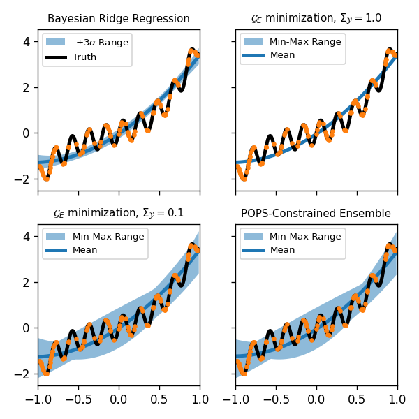
Figure 1: Regression of a deterministic quadratic polynomial ($P=3$) model onto a sinusoidal ”simulation engine”, trained on $N=100$ points. Clockwise from top left: mean and $3\sigma$ confidence interval from Bayesian ridge regression , direct minimization of $\mathcal{G}_{E}$, regularized with $\Sigma_{\mathcal{Y}}=1$, the min/max range of the POPS-ensemble (21), and $\mathcal{G}_{E}$ with $\Sigma_{\mathcal{Y}}=0.1$.

We applied the same procedure to a model system with $P=6$ decorrelated features, unlike the polynomial example, to simulate more realistic datasets. The minimization routine could only treat a small range of $\Sigma_{\mathcal{Y}}$ values, which we normalize by the loss minimizer RMS error $\sigma_{MLE}$. Figure 2 shows the resulting parameter distributions. At large $\Sigma_{\mathcal{Y}}$ the minimizer quickly concentrates all ensemble members on the minimum loss solution, whilst at $\Sigma_{\mathcal{Y}}=\sigma_{MLE}$ the final distribution is very close to the POPS-ensemble. At lower values the final distribution was a little broader, but we attribute this largely to numerical instabilities as the final result is sensitive to initial conditions (unlike the first two cases). In addition, a minimizer initialized with the POPS-ensemble did not change appreciably. These albeit simple results give strong evidence that the POPS-ensemble is indeed a stable and highly efficient means to find approximate minimizers of ${\mathcal{G}}$ that would otherwise be intractable.

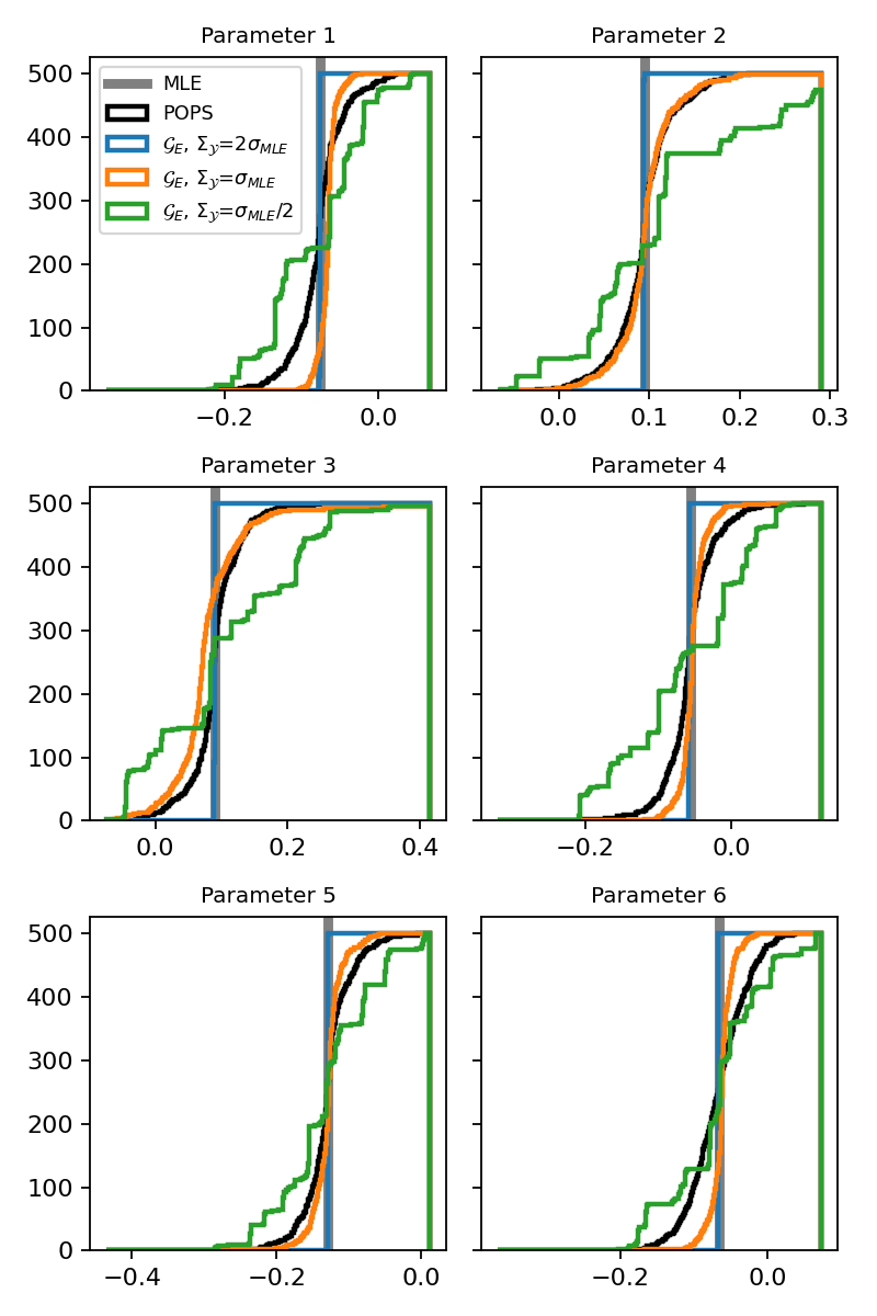
Figure 2: Regression of a $P=6$ linear model onto a cubic ”simulation engine”, trained on $N=500$ points. The panels show the culmulative distribution of each parameter across the ensemble (same size as $N$) for the loss minimizer (MLE), the POPS-ensemble (21) and from direct minimization of ${\mathcal{G}}$ with $\Sigma_{\mathcal{Y}}/\sigma_{MLE}=2,1,1/2$.

IV.2 Test errors in medium-dimensional linear regression

We now look at higher/medium dimensional problems, $P=10-100$, where direct minimization of ${\mathcal{G}}$ is not practical. The simulation engines (see supplementary material) were constrained to be misspecified from the linear surrogate models by combining features in quadratic, cubic or sinusoidal functions or randomly sampling the linear feature coefficients from some predetermined subset of models. A noise term that simulates the presence of variability orthogonal to the chosen feature set was also used. In all cases, independent test and training data were generated, typically with a 10:90 test:train split. However, all conclusions remain robust to varying the precise nature of data generation and the classes of engine considered. Additional examples are provided in the supplementary material and appendix C.

IV.2.1 POPS-ensemble prediction of test errors

For each test point, it is simple to generate an ‘envelope’, or max/min range, from the POPS-ensemble. We find this envelope provides a highly informative bound on test errors for large $N/P$. The top left of figure 3 is a parity plot for the minimum loss model, showing around 93% coverage, or 7% envelope violation. The violation rate drops with $N/P$, as shown on the bottom of figure 3 for a range of $P$ and $N/P$ and two simulation engines.

Whilst the envelope bounds are highly informative, it is also desirable to predict test error distributions. As discussed above, the limitation of our POPS-ensemble is that the weighting of ensemble members is unlikely to be optimal, whilst the max/min range can be expected to be robust. As a result, a conservative estimate of the test error can be generated by uniformly resampling the max/min bounds for each test point to generate predicted error histograms. As shown in the top (right) of figure 3, this prediction from the POPS-ensemble results in excellent agreement with the test error ensemble, as confirmed across multiple engines in appendix A. Whilst a single (re)sample per test point is sufficient, it is possible to effectively bootstrap error histograms through repeated resampling.

IV.2.2 Resampled POPS (rPOPS) ensemble

The parameter vectors of the POPS-ensemble across all simulation engines studied are observed to be dense across their simplex, or hypercube of the max/min range per parameter. Inspired by the success of the uniform resampling approach used to produce test error predictions of the POPS ensemble in figure 3, we have also investigated the effect of uniformly resampling this ‘POPS-simplex’, a process we name as ‘resampled’ POPS, or rPOPS. We emphasize that the rPOPS approach makes a strong assumption that all parameter vectors inside the POPS- simplex are close to valid POPS-ensemble members. We thus include these results as a motivation for further study; in particular, whilst the $\mathcal{O}(N)$ cost of the POPS-ensemble remains highly managable, the cost of the rPOPS-ensemble can be tailored through the number of resamples, offering large efficiencies as $N/P\to\infty$ when producing envelopes and test error distributions.

As shown in figure 3, the rPOPS results are excellent, giving tight agreement with test error distributions and only slightly more conservative errors bounds, a feature which is again robust across simulation engines (appendix C). A detailed investigation of the POPS-simplex and theoretical analysis of the rPOPS-ensemble is left as a topic for future study. We conclude with an application to challenging high-dimensional $P=\mathcal{O}(1000)$ datasets from atomic machine learning.

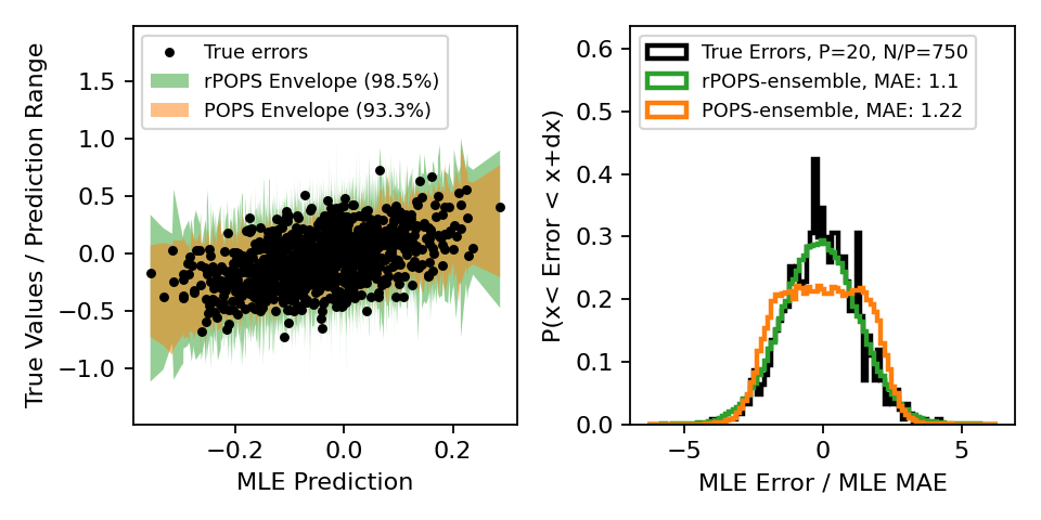
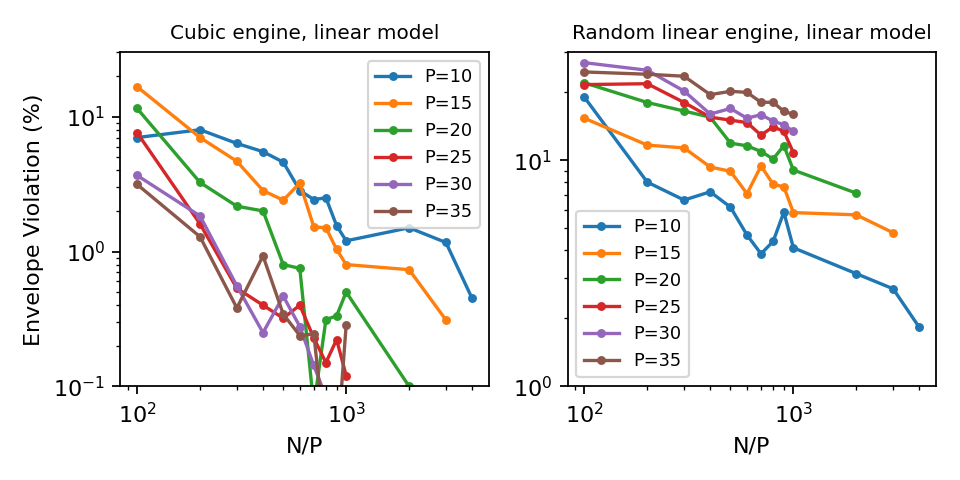
Figure 3: Top: test error predictions for a misspecified linear surrogate model (P=20) on a cubic simulation engine. Left: parity plot for the minimum loss model, along with envelope bounds from the POPS-ensemble and rPOPS-ensemble (see text), showing 93-98% coverage at $N/P=750$. Right: Test error histogram, along with predicted test errors from the POPS- and rPOPS-ensemble, as explained in the text. Below: POPS-ensemble envelope violation rates with $P$ and $N/P$ for two simulation engines.

IV.3 Interatomic potentials for material simulations

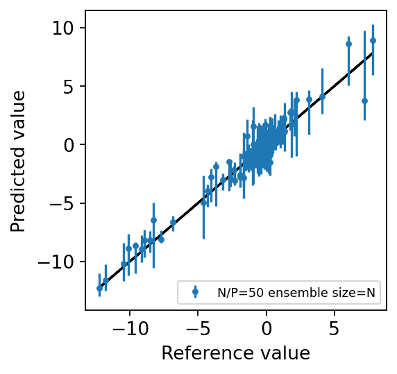
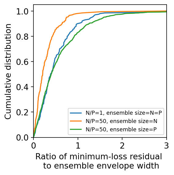
Figure 4: Characteristics of the ensemble method for the application to interatomic potentials. Left: Parity plot for energy and force predictions for $N/P=50$. The errorbars reflect the min/max envelope of the POPS-ensemble. Right: cumulative distribution of the ratio of the residual of the minimum-loss model to the envelope width (max/min range per test point) for different conditions.

Atomic-scale simulations of materials were traditionally broadly classified into two types:

• Empirical simulations with physically-motivated parametric models of interatomic interactions. These allow for large simulations over long timescales at a qualitative level of accuracy.

• First-principle quantum simulations where interatomic interactions are obtained from approximate solutions of the full Schrodinger equation. Such calculations can provide quantitative predictions at a high computational cost that strongly limits the accessible time- and length-scales.

The advent of machine learning has blurred the lines between these two categories by promising near-quantum accuracy at a much more favorable computational cost and scaling (typically cubic in the number of atoms for first-principles, and linear for empirical approaches) (Deringer et al., 2019). In the most common approaches, the total energy of the system of atoms $V$ is factored into a sum of per-atom contributions $V_{i}$, which are themselves parameterized in term of a vector of features that describe the local atomic environment around each atom ${\bf F}_{i}(\{{\bf x}_{j}|r_{ij}<r_{c}\})$, where $r_{c}$ is a interaction range. Training an ML model then proceeds by minimizing a squared error loss between the energies and forces (which are given by elements of the negative gradient of the total energy, $-\nabla V$) as obtained by first-principle methods and those predicted by the ML model. While certain ML approaches are in principle systematically improvable, the computational cost associated with evaluating energies and forces repeatedly for large systems and long times often limits the complexity of the models that are selected for applications. Further, quantum calculations can be tightly converged, so that their intrinsic error $\epsilon$ (w.r.t. a fully converged version of the same calculation) can be made small compared to typical errors incurred by the models that are selected in practice. This regime corresponds to the underparametrized deterministic limit considered above. Estimating the errors incurred by ML models of interatomic interactions (Wen and Tadmor, 2020; Li et al., 2018; Gabriel et al., 2021; Wan et al., 2021) is required when one wishes to assess the robustness of conclusions drawn from the simulations, especially when quantitative predictions are sought.

In the following, training data was generated using an information-theoretic approach (Karabin and Perez, 2020; Montes de Oca Zapiain et al., 2022) that maximizes the information entropy of the training data distribution, as measured in feature space. 10,000 atomistic configurations containing between 2 and 32 tungsten atoms were generated and characterized using Density Functional Theory (Kohn and Sham, 1965), yielding 167,922 training data points in total (10,000 energies and 157,922 force components, 3 Cartesian for each atom in every configuration).

Per-atom energies are expressed as a linear combination of $P=1596$ so-called bispectrum components within the ‘Quadratic’ Spectral Neighborhood Analysis Potential (SNAP) formalism (Wood and Thompson, 2018), giving the linear surrogate model $V_{i}={\bm{\Theta}}\cdot{\bf F}_{i}(\{{\bf x}_{j}|r_{ij}<r_{c}\})$.

Numerical experiments were carried out by randomly sub-selecting $N$ training points (either energies or gradient components), and by generating a discrete ensemble of $N$ pointwise-optimal models according to Eq. 21. The properties of the ensemble are then evaluated on a complementary set of 1,000 randomly-selected testing points (again either energies or gradient components). The random test/train partition is repeated 10 times for each value of $N/P$.

The results show that the envelope violation on test data varies between $40\%$ and $10\%$ for $N/P=1$ and $50$, respectively, in qualitative agreement with the results shown in figure 3, demonstrating that worst-case model errors are increasingly well captured by the ensemble envelope. Indeed, the scaling is actually superior to the medium test examples. As seen in these examples, the envelope induced by the model ensemble yields a useful estimate of the actual errors, e.g., as incurred by the ordinary minimum-loss model, as reported in figure 4. For example, the mean ratio of the residual of the minimum-loss model to the envelope width (max/min range) is around $0.45$ at $N/P=1$, i.e, the envelope width overestimates the actual minimum-loss residual only by a factor of around 2 on average. This figure drops to about $0.25$ at $N/P=50$, following the broadening of the envelopes that occurs as rare ”outliers” that are particularly difficult to capture within the model class are gradually added to the training set. This was empirically verified by sampling ensembles containing only $P$ models, independently of the size of the training set: in this case, the mean ratio of the residual of the minimum-loss model to the envelope width remains around $0.45$ (c.f., figure 4). This numerical experiment indicates that the width of the model envelope predictions provides reliable worst-case confidence intervals as well as representative (albeit somewhat conservative) estimates of the actual errors at testing points.

This information thus generated is invaluable to estimate the uncertainties on physical quantities inferred from simulations that encounter local atomic environments that significantly differ from those contained in the training set. We however note that accurate uncertainty quantification relies on the training sets being representative of possible testing sets, which highlights the fundamental importance training data diversity (Karabin and Perez, 2020) and the perils of narrowly tailored training sets.

V Conclusion

In spite of its ubiquity in practical applications, misspecification is often ignored in Bayesian regression approaches based on expected loss minimization, which can lead to erroneous conclusions regarding parameter uncertainty quantification, surrogate model selection, and error propagation. In this work, we show that the important near-deterministic underparameterized regime is amenable to approximation by a formally simple discrete ensemble ansatz that exploits the concentration of the cross-entropy minimizing ensemble onto pointwise optimal parameter sets. For linear regression problems, this ensemble can be obtained extremely efficiently using rank-one perturbations of the expected loss solution. POPS-constrained loss-minimizing ensembles are shown to produce excellent parameter distributions, worst-case bounds on model predictions, and approximations of the pointwise errors.

Software and Data

Will be released after peer review

Appendix A Model selection criteria for deterministic models

The Bayesian information criterion (BIC), used to discriminate between possible surrogate models, is derived by approximating (twice) the negative log evidence as $N/P\to\infty$, assuming a slowly varying prior $\pi_{0}({\bm{\Theta}})=\mathcal{O}(1)$. Using the above definitions we find

$$BIC=-2\ln\left|\int\exp(-N\hat{L}({{\bm{\Theta}}}))\pi_{0}({\bm{\Theta}}){\rm d}{\bm{\Theta}}\right|\to N{\rm Tr}({\bm{\Sigma}}^{*}_{\mathcal{L}}{\bm{\Sigma}}^{-1}_{\mathcal{Y}})+\ln\left(\|{\bm{\Sigma}}_{\mathcal{Y}}\|^{N}N^{P}\|{\bm{\mathcal{I}}}^{*}_{\mathcal{L}}\|\right)+\mathcal{O}(1).$$ (22)

We note that the value of the PAC-Bayes loss bound (8) satifies $BIC=2N\hat{\mathcal{L}}_{N}[\pi_{{\mathcal{L}},N}]-2C_{0}$, with $C_{0}$ model independent. In standard derivations ${\bm{\Sigma}}_{\mathcal{Y}}$ is set to the variational maximum likelihood solution ${\bm{\Sigma}}_{\mathcal{Y}}={\bm{\Sigma}}^{*}_{\mathcal{L}}$, yielding the familar expression $BIC=P\ln N+N\ln\|{\bm{\Sigma}}^{*}_{\mathcal{L}}\|+\ln\|{\bm{\mathcal{I}}}^{*}_{\mathcal{L}}\|$, where model independent terms are neglected. However, for deterministic regression problems, ${\bm{\Sigma}}_{\mathcal{Y}}$ is fixed. Neglecting model-independent terms, this gives an alternative BIC for deterministic models of

$$BIC=N{\rm Tr}({\bm{\Sigma}}^{*}_{\mathcal{E}}{\bm{\Sigma}}^{-1}_{\mathcal{Y}})+P\ln N+\ln\|{\bm{\mathcal{I}}}^{*}_{\mathcal{L}}\|.$$ (23)

Appendix B POPS-constrained variational ansatz for PAC-Bayesian linear regression

The POPS-constrained ensemble ansatz can also be used to incorporate both epistemic and misspecification parameter uncertainties in a variational scheme robust at small $N/P$, which we detail here for completeness. We assume a Gaussian posterior $\pi_{V}({\bm{\Theta}})=\mathcal{N}({\bm{\Theta}}|{\bm{\mu}}_{V},{\bm{\Sigma}}_{V})$, such that the ensemble ansatz is characterized by the ensemble mean ${\bm{\mu}}_{E}=\langle{\bm{\Theta}}^{*}_{\mathbf{X}}\rangle$ and covariance ${\bm{\Sigma}}_{E}$. A first approximation simply combines the covariance from minimization of the PAC-Bayes loss bound (8), ${\bm{\Sigma}}^{*}_{\mathcal{L}}=\left[{\bm{\Sigma}}_{\mathcal{Y}}{\bm{\Sigma}}^{-1}_{0}+N\langle{\mathbf{F}}({\mathbf{X}})[{\mathbf{F}}({\mathbf{X}})]^{\top}\rangle_{\mathcal{X}}\right]^{-1}$, with the ensemble covariance ${\bm{\Sigma}}_{E}$. This yield a posterior covariance ${\bm{\Sigma}}^{*}_{\mathcal{L}}+{\bm{\Sigma}}_{E}$, which remains robust at finite $N/P$ and limits to ${\bm{\Sigma}}_{E}$ as $N/P\to\infty$.

However, the full variational scheme has comparable complexity to Bayesian ridge regression for linear models [Tipping, 2001]. Our variational ansatz replaces ${\bm{\Theta}}^{*}_{\mathcal{L}}$ in the pointwise fits (21) with a variational parameter ${\bm{\Theta}}_{V}$, giving a variational posterior mean and covariance of

$${\bm{\mu}}_{V}({\bm{\Theta}}_{V})\equiv\left\langle{\bf v}_{\mathbf{X}}\right\rangle_{\mathcal{X}}+\left\langle{\bf W}_{\mathbf{X}}\right\rangle_{\mathcal{X}}{\bm{\Theta}}_{V},\quad{\bm{\Sigma}}_{V}({\bm{\Theta}}_{V})\equiv\left\langle\left[\delta{\bf v}_{\mathbf{X}}+\delta{\bf W}_{\mathbf{X}}{\bm{\Theta}}_{V}\right]\left[\delta{\bf v}_{\mathbf{X}}+\delta{\bf W}_{\mathbf{X}}{\bm{\Theta}}_{V}\right]^{\top}\right\rangle_{\mathcal{X}},$$ (24)

where ${\bf v}_{\mathbf{X}},{\bf W}_{\mathbf{X}}$ are derived from (21) such that ${\bm{\mu}}_{V}({\bm{\Theta}}^{*}_{\mathcal{L}})={\bm{\mu}}_{E}$ and ${\bm{\Sigma}}_{V}({\bm{\Theta}}^{*}_{\mathcal{L}})={\bm{\Sigma}}_{E}$, reading

$${\bf v}_{\mathbf{X}}\equiv{\bf A}\frac{{\mathbf{F}}({\mathbf{X}}){\mathcal{E}}({\mathbf{X}})}{{\rm h}({\mathbf{X}})},\quad{\bf W}_{\mathbf{X}}\equiv\mathbb{I}-{\bf A}\frac{{\mathbf{F}}({\mathbf{X}}){\mathbf{F}}^{\top}({\mathbf{X}})}{{\rm h}({\mathbf{X}})},\quad\delta{\bf v}_{\mathbf{X}}\equiv{\bf v}_{\mathbf{X}}-\left\langle{\bf v}_{\mathbf{X}}\right\rangle_{\mathcal{X}},\quad\delta{\bf W}_{\mathbf{X}}\equiv{\bf W}_{\mathbf{X}}-\left\langle{\bf W}_{\mathbf{X}}\right\rangle_{\mathcal{X}}.$$

This gives a variational distribution which can be used in the PAC-Bayes loss bound $\hat{{\mathcal{L}}}_{N}[\pi]$ (8)

$$\pi_{V}({\bm{\Theta}}|{\bm{\Theta}}_{V})\equiv\mathcal{N}({\bm{\Theta}}|{\bm{\mu}}_{V}({\bm{\Theta}}_{V}),{\bm{\Sigma}}_{V}({\bm{\Theta}}_{V})),\quad{\bm{\Theta}}_{V}^{*}\equiv\arg\min_{{\bm{\Theta}}_{V}\in{\mathcal{P}}}\hat{{\mathcal{L}}}_{N}[\pi_{V}(.|{\bm{\Theta}}_{V})].$$ (25)

Using the empirical loss $\hat{L}_{N}({\bm{\Theta}})$, quadratic in ${\bm{\Theta}}$ for linear models, the variational minimum satisfies

$$\left\langle{\bf W}_{\mathbf{X}}\right\rangle_{\mathcal{X}}[N{\bm{\nabla}}_{\bm{\Theta}}\hat{L}_{N}({\bm{\Theta}}^{*}_{V})+{\bm{\Sigma}}_{0}^{-1}{\bm{\mu}}_{V}({\bm{\Theta}}^{*}_{V})]+\left[N{\bf A}^{-1}+{\bm{\Sigma}}_{0}^{-1}+{\bm{\Sigma}}^{-1}_{V}({\bm{\Theta}}^{*}_{V})\right]:{\bm{\Sigma}}^{\prime}_{V}({\bm{\Theta}}^{*}_{V})={\bf 0},$$ (26)

where $:$ denotes a contraction over the first two indicies of a third-order tensor ${\bm{\Sigma}}^{\prime}_{V}({\bm{\Theta}})$ linear in ${\bm{\Theta}}$:

$${\bm{\Sigma}}^{\prime}_{V}({\bm{\Theta}})=\left\langle\delta{\bf W}_{\mathbf{X}}\delta{\bf v}^{\top}_{\mathbf{X}}+\delta{\bf v}_{\mathbf{X}}\delta{\bf W}_{\mathbf{X}}+\delta{\bf W}_{\mathbf{X}}{\bm{\Theta}}\delta{\bf W}_{\mathbf{X}}+\delta{\bf W}_{\mathbf{X}}\delta{\bf W}_{\mathbf{X}}{\bm{\Theta}}\right\rangle_{\mathcal{X}}.$$ (27)

As for Bayesian ridge regression, the only non-linearity in (26) is the term ${\bm{\Sigma}}^{-1}_{V}({\bm{\Theta}}):{\bm{\Sigma}}^{\prime}_{V}({\bm{\Theta}}^{*}_{V})$, meaning any implementation can use existing iterative schemes e.g. [Tipping, 2001],[Wipf and Nagarajan, 2007]. A full study of the low data regime is left for future work.

Appendix C Additional plots of test error prediction

The plots below are identical in presentation to the top row of figure 3, but for the quadratic and random linear simulation engines described in the main text.

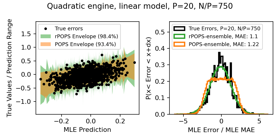
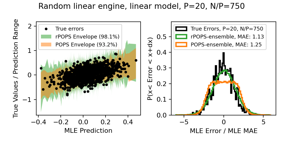
Figure 5: Test error prediction for medium dimensional problems. From left: Observed test errors for a misspecified linear surrogate model (P=20) on a quadratic simulation engine, along with predicted test errors from the POPS-ensemble. Parity plots for the minimum loss model, along with envelope bounds from the POPS-ensemble.

References

- Alizadeh et al. (2020) Reza Alizadeh, Janet K Allen, and Farrokh Mistree. Managing computational complexity using surrogate models: a critical review. Research in Engineering Design, 31:275–298, 2020.
- Alquier (2021) Pierre Alquier. User-friendly introduction to pac-bayes bounds. arXiv preprint arXiv:2110.11216, 2021.
- Bonatti et al. (2022) Colin Bonatti, Bekim Berisha, and Dirk Mohr. From cp-fft to cp-rnn: Recurrent neural network surrogate model of crystal plasticity. International Journal of Plasticity, 158:103430, 2022.
- Deringer et al. (2019) Volker L Deringer, Miguel A Caro, and Gábor Csányi. Machine learning interatomic potentials as emerging tools for materials science. Advanced Materials, 31(46):1902765, 2019.
- Gabriel et al. (2021) Joshua J Gabriel, Noah H Paulson, Thien C Duong, Francesca Tavazza, Chandler A Becker, Santanu Chaudhuri, and Marius Stan. Uncertainty quantification in atomistic modeling of metals and its effect on mesoscale and continuum modeling: A review. JOM, 73:149–163, 2021.
- Germain et al. (2016) Pascal Germain, Francis Bach, Alexandre Lacoste, and Simon Lacoste-Julien. Pac-bayesian theory meets bayesian inference. Advances in Neural Information Processing Systems, 29, 2016.
- Hoeffding (1994) Wassily Hoeffding. Probability inequalities for sums of bounded random variables. The collected works of Wassily Hoeffding, pages 409–426, 1994.
- Imbalzano et al. (2021) Giulio Imbalzano, Yongbin Zhuang, Venkat Kapil, Kevin Rossi, Edgar A Engel, Federico Grasselli, and Michele Ceriotti. Uncertainty estimation for molecular dynamics and sampling. The Journal of Chemical Physics, 154(7), 2021.
- Karabin and Perez (2020) Mariia Karabin and Danny Perez. An entropy-maximization approach to automated training set generation for interatomic potentials. The Journal of Chemical Physics, 153(9), 2020.
- Kato et al. (2022) Yuko Kato, David MJ Tax, and Marco Loog. A view on model misspecification in uncertainty quantification. arXiv preprint arXiv:2210.16938, 2022.
- Kohn and Sham (1965) W. Kohn and L. J. Sham. Self-consistent equations including exchange and correlation effects. Phys. Rev., 140:A1133–A1138, Nov 1965. doi: 10.1103/PhysRev.140.A1133. URL https://link.aps.org/doi/10.1103/PhysRev.140.A1133.
- Lahlou et al. (2021) Salem Lahlou, Moksh Jain, Hadi Nekoei, Victor Ion Butoi, Paul Bertin, Jarrid Rector-Brooks, Maksym Korablyov, and Yoshua Bengio. Deup: Direct epistemic uncertainty prediction. arXiv preprint arXiv:2102.08501, 2021.
- Lapointe et al. (2020) Clovis Lapointe, Thomas D Swinburne, Louis Thiry, Stéphane Mallat, Laurent Proville, Charlotte S Becquart, and Mihai-Cosmin Marinica. Machine learning surrogate models for prediction of point defect vibrational entropy. Physical Review Materials, 4(6):063802, 2020.
- Li et al. (2018) Yumeng Li, Weirong Xiao, and Pingfeng Wang. Uncertainty quantification of artificial neural network based machine learning potentials. In ASME International Mechanical Engineering Congress and Exposition, volume 52170, page V012T11A030. American Society of Mechanical Engineers, 2018.
- Lotfi et al. (2022) Sanae Lotfi, Pavel Izmailov, Gregory Benton, Micah Goldblum, and Andrew Gordon Wilson. Bayesian model selection, the marginal likelihood, and generalization. In International Conference on Machine Learning, pages 14223–14247. PMLR, 2022.
- Mahalanobis (1936) Prasanta Chandra Mahalanobis. On the generalized distance in statistics. In Procedings of the National Institute of Science of India. National Institute of Science of India, 1936.
- Masegosa (2020) Andres Masegosa. Learning under model misspecification: Applications to variational and ensemble methods. Advances in Neural Information Processing Systems, 33:5479–5491, 2020.
- Montes de Oca Zapiain et al. (2022) David Montes de Oca Zapiain, Mitchell A Wood, Nicholas Lubbers, Carlos Z Pereyra, Aidan P Thompson, and Danny Perez. Training data selection for accuracy and transferability of interatomic potentials. npj Computational Materials, 8(1):189, 2022.
- Morningstar et al. (2022) Warren R Morningstar, Alex Alemi, and Joshua V Dillon. Pacm-bayes: Narrowing the empirical risk gap in the misspecified bayesian regime. In International Conference on Artificial Intelligence and Statistics, pages 8270–8298. PMLR, 2022.
- Nyshadham et al. (2019) Chandramouli Nyshadham, Matthias Rupp, Brayden Bekker, Alexander V Shapeev, Tim Mueller, Conrad W Rosenbrock, Gábor Csányi, David W Wingate, and Gus LW Hart. Machine-learned multi-system surrogate models for materials prediction. npj Computational Materials, 5(1):51, 2019.
- Psaros et al. (2023) Apostolos F Psaros, Xuhui Meng, Zongren Zou, Ling Guo, and George Em Karniadakis. Uncertainty quantification in scientific machine learning: Methods, metrics, and comparisons. Journal of Computational Physics, 477:111902, 2023.
- Tipping (2001) Michael E Tipping. Sparse bayesian learning and the relevance vector machine. Journal of machine learning research, 1(Jun):211–244, 2001.
- Tsybakov (2008) Alexandre B. Tsybakov. Introduction to Nonparametric Estimation. Springer Publishing Company, Incorporated, 1st edition, 2008. ISBN 0387790519.
- Wan et al. (2021) Shunzhou Wan, Robert C Sinclair, and Peter V Coveney. Uncertainty quantification in classical molecular dynamics. Philosophical Transactions of the Royal Society A, 379(2197):20200082, 2021.
- Wen and Tadmor (2020) Mingjian Wen and Ellad B Tadmor. Uncertainty quantification in molecular simulations with dropout neural network potentials. npj computational materials, 6(1):124, 2020.
- Wipf and Nagarajan (2007) David Wipf and Srikantan Nagarajan. A new view of automatic relevance determination. Advances in neural information processing systems, 20, 2007.
- Wood and Thompson (2018) Mitchell A Wood and Aidan P Thompson. Extending the accuracy of the snap interatomic potential form. The Journal of chemical physics, 148(24), 2018.